SM Feynman diagrams mediating (top) the $ B ^0_ s \rightarrow \mu ^+ \mu ^- $ and (bottom) the $ B ^0_ s \rightarrow \mu ^+ \mu ^- \gamma $ processes. Subpanels show (a) the so-called "penguin" diagram and (b) the "box" diagram for $ B ^0_ s \rightarrow \mu ^+ \mu ^- $ , and (c) an ISR contribution and (d) an FSR contribution to $ B ^0_ s \rightarrow \mu ^+ \mu ^- \gamma $ .

BDT distribution calibrated using corrected simulated $ B ^0_ s \rightarrow \mu ^+ \mu ^- $ decays (black circles) and combinatorial background from high dimuon-mass data sidebands (blue filled circles) in (left) Run 1 and (right) Run 2 data. Blue error bands represent the statistical uncertainty.

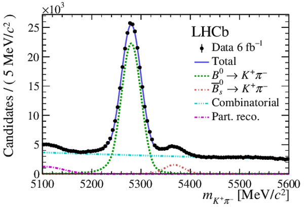
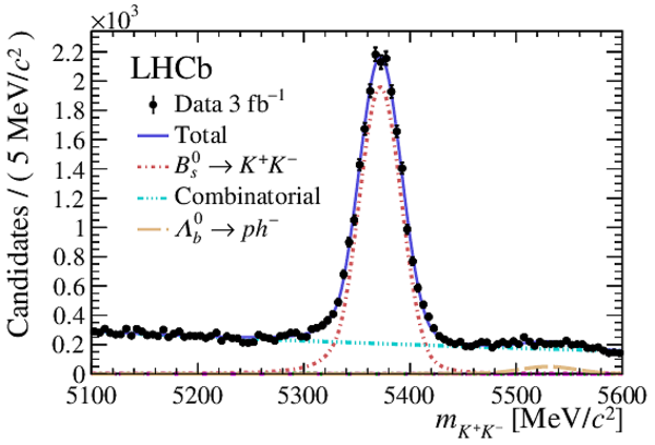
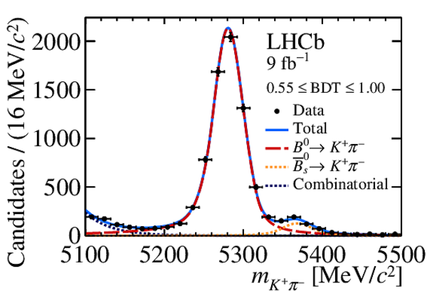
Mass distributions of selected (top) $ B ^0 \rightarrow K ^+ \pi ^- $ and (bottom) $ B ^0_ s \rightarrow K ^+ K ^- $ candidates in (left) Run 1 and (right) Run 2 data. The results of the fits used to determine the means of the $ B _{( s )}^0 \rightarrow \mu ^+ \mu ^- $ mass distributions are overlaid and the different components are detailed in the legends.

Mass distributions of (top) $ { J \mskip -3mu/\mskip -2mu\psi } \rightarrow \mu^+\mu^-$, (centre) $\psi{(2S)} \rightarrow \mu^+\mu^-$, (bottom) $\varUpsilon(1S,2S,3S)\rightarrow \mu^+\mu^-$ candidates in (left) Run 1 and (right) Run 2 data. The result from the fit to determine the mass resolutions to each sample is overlaid, and the components are detailed in the legend.

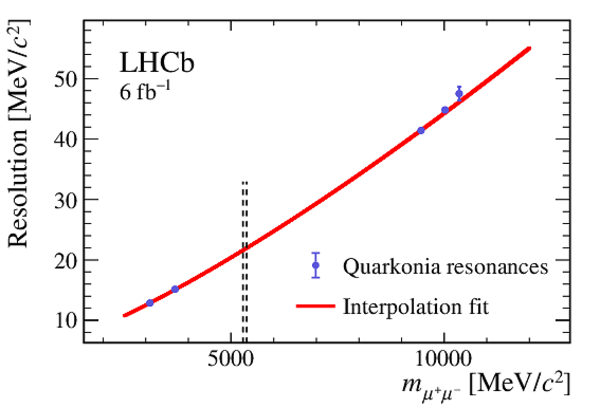
Fit to the measured mass resolutions of quarkonia resonances (blue dots) to obtain the mass resolution at the $ B ^0$ and $ B ^0_ s $ masses as indicated by the two dashed lines in (left) Run 1 and (right) Run 2 data.

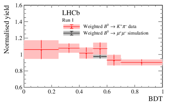
The calibrated BDT distribution for $ B ^0_ s \rightarrow \mu ^+ \mu ^- $ decays with $ A^{\mu\mu}_{\Delta\Gamma_s} =1$ (black) and $ B ^0 \rightarrow \mu ^+ \mu ^- $ decays (red) for (left) Run 1 and (right) Run 2, including the total uncertainty on the fraction per BDT region. The $ B ^0_ s \rightarrow \mu ^+ \mu ^- $ and $ B ^0 \rightarrow \mu ^+ \mu ^- $ distributions are determined on corrected simulated samples, as described in the text.

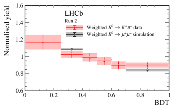
The BDT distributions of (top) $ B ^0_ s \rightarrow \mu ^+ \mu ^- $ and $ B ^0_ s \rightarrow K ^+ K ^- $ decays and (bottom) $ B ^0 \rightarrow \mu ^+ \mu ^- $ and $ B ^0 \rightarrow K ^+ \pi ^- $ decays in (left) Run 1 and (right) Run 2 data, including the total uncertainty on the fraction per BDT region. For $ B ^0_ s \rightarrow \mu ^+ \mu ^- $ and $ B ^0 \rightarrow \mu ^+ \mu ^- $ decays, the distributions are determined on corrected simulated samples, as described in the text, and are shown in black. The $ B ^0_ s \rightarrow K ^+ K ^- $ and $ B ^0 \rightarrow K ^+ \pi ^- $ distributions are determined using fits to data as described in the text and are shown in red.

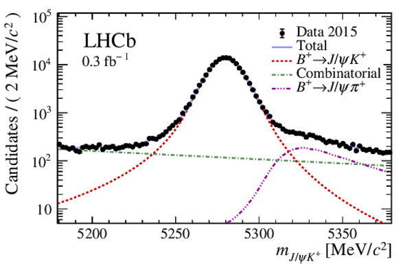
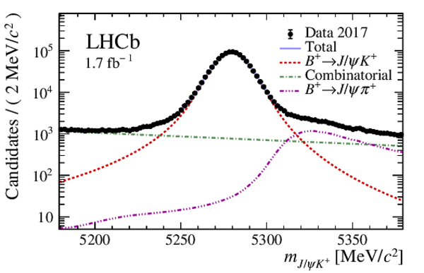
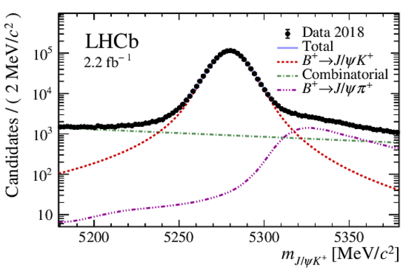
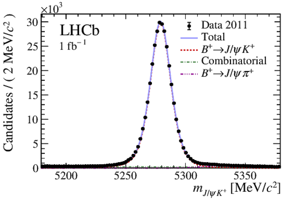
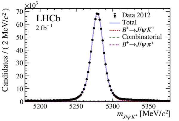
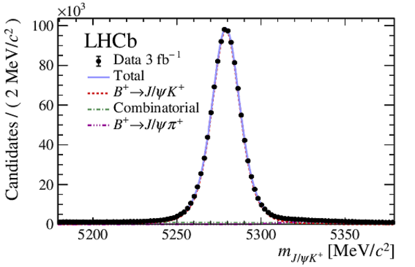
Mass distribution of $ B ^+ \rightarrow { J \mskip -3mu/\mskip -2mu\psi } K ^+ $ candidates in data for different data-taking years. Superimposed is a fit to the distribution: the blue line shows the total fit, the red dashed line is the $ B ^+ \rightarrow { J \mskip -3mu/\mskip -2mu\psi } K ^+ $ component, the green dash-dotted line is the combinatorial background, the purple dash-three-dotted line is the $ B ^+ \rightarrow { J \mskip -3mu/\mskip -2mu\psi } \pi ^+ $ misidentified background.

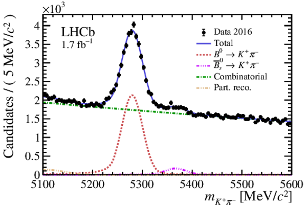
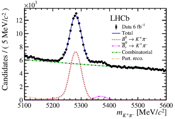
Mass distribution of $ B ^0 \rightarrow K ^+ \pi ^- $ candidates in data for different data-taking years, triggered independently of the signal. Superimposed is a fit to the distribution: the blue line shows the total fit, the red dashed line is the $ B ^0 \rightarrow K ^+ \pi ^- $ component, the magenta dashed line is the $\overline{ B } {}^0_ s \rightarrow K ^+ \pi ^- $ component, the green dashed line is the combinatorial background, and the brown dashed line is the partially reconstructed background component.

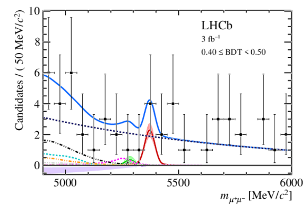
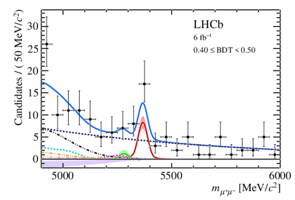
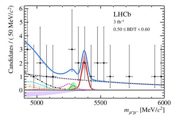
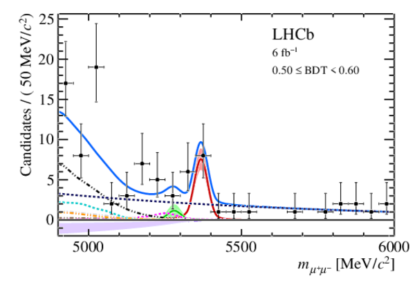
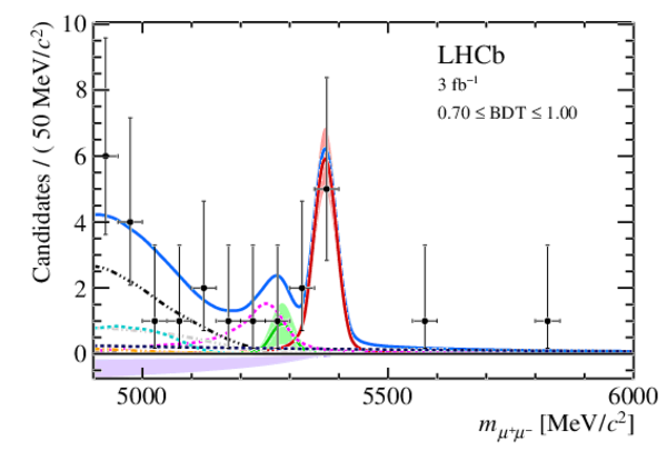
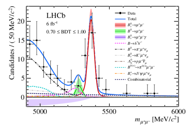
Mass distribution of signal candidates (black dots) for (left) Run 1 and (right) Run 2 samples in regions of BDT. The result of the fit is overlaid (blue line) and the different components detailed in the legend. The solid bands represent the variation of the signal branching fractions within their total uncertainty.

Two-dimensional representations of the branching fraction measurements for the decays (top) $ B ^0_ s \rightarrow \mu ^+ \mu ^- $ and $ B ^0 \rightarrow \mu ^+ \mu ^- $ , (bottom left) $ B ^0 \rightarrow \mu ^+ \mu ^- $ and $ B ^0_ s \rightarrow \mu ^+ \mu ^- \gamma $ and (bottom right) $ B ^0_ s \rightarrow \mu ^+ \mu ^- $ and $ B ^0_ s \rightarrow \mu ^+ \mu ^- \gamma $ . The $ B ^0_ s \rightarrow \mu ^+ \mu ^- \gamma $ branching fraction is limited to the range $m_{\mu\mu}>4.9\text{ Ge V /}c^2 $. The measured central values of the branching fractions are indicated with a blue dot. The profile likelihood contours for 68%, 95% and 99% CL regions of the result presented in this paper are shown as blue contours, while in the top plot the brown contours indicate the previous measurement [32] and the red cross shows the SM prediction. Figure reproduced from Ref. [37].

Results from the CL$_{\text{s}}$ scan used to obtain the limit on (left) $\cal B ( B ^0 \rightarrow \mu ^+ \mu ^- )$ and (right) $\cal B ( B ^0_ s \rightarrow \mu ^+ \mu ^- \gamma )$. The background-only expectation is shown by the red line and the 1$\sigma$ and 2$\sigma$ bands are shown as light blue and blue bands respectively. The observation is shown as the solid black line. The two dashed lines intersecting with the observation indicate the limits at 90% and 95% CL for the upper and lower line, respectively.

Dimuon mass distributions of $ B ^0_ s \rightarrow \mu ^+ \mu ^- $ candidates with the fit model used to perform the background subtraction for the measurement of the $ B ^0_ s \rightarrow \mu ^+ \mu ^- $ effective lifetime superimposed in the (left) low and (right) high BDT regions.

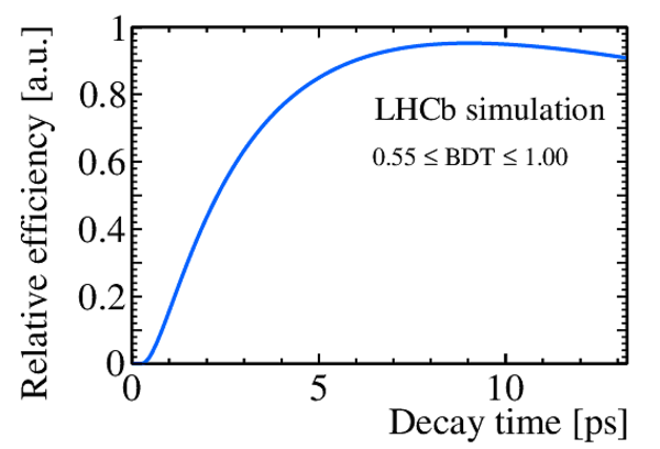
The functions used to model the decay-time efficiency in the (left) low and (right) high BDT regions in the fit for the $ B ^0_ s \rightarrow \mu ^+ \mu ^- $ effective lifetime.

(Top) Distribution of $ K ^+ K ^- $ mass with the fit models used to perform the background subtraction superimposed and (bottom) the background-subtracted decay-time distributions with the fit model used to determine the $ B ^0_ s \rightarrow K ^+ K ^- $ effective lifetime superimposed (bottom row). The distributions in the low and high BDT regions are shown in the left and right columns, respectively.

(Top) Distribution of $ K ^+ \pi ^- $ mass with the fit models used to perform the background subtraction superimposed and (bottom) the background-subtracted decay-time distributions with the fit model used to determine the $ B ^0 \rightarrow K ^+ \pi ^- $ lifetime superimposed. The distributions in the low and high BDT regions are shown in the left and right columns, respectively.

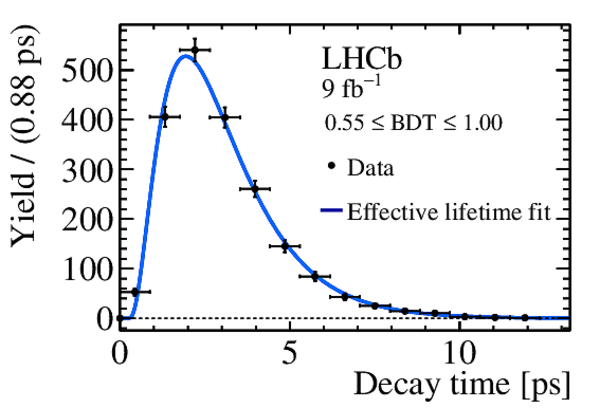
Background-subtracted decay-time distributions with the fit model used to extract the $ B ^0_ s \rightarrow \mu ^+ \mu ^- $ effective lifetime superimposed in the (left) low and (right) high BDT regions.

Animated gif made out of all figures.

Luminosity-weighted signal mass shape parameter combinations per data set, including propagated uncertainties. Where appropriate, statistical and systematic uncertainties are added in quadrature. As the tail parameters determined in Run 1 and Run 2 are consistent, they are combined into common estimates.

Yields of the two normalisation channels with their combined statistical and systematic errors.

Efficiencies of reconstruction within the LHCb detector and selection for the signal and normalisation channels, averaged for the two running periods. The uncertainties include the statistical uncertainty from the simulated samples and the uncertainty of the tracking efficiency corrections.

Particle identification efficiencies for the signal and normalisation channels, averaged for the two running periods, where the first uncertainty is statistical and the second systematic. A data-simulation correction of the muon-system identification is included for channels with muons. For the $ B ^+ \rightarrow { J \mskip -3mu/\mskip -2mu\psi } K ^+ $ channel only the data-simulation correction part of the muon identification is reported, as no multivariate PID requirement is applied to this channel.

Trigger efficiencies for the signal and normalisation channels, averaged for the two data taking periods. The first uncertainty is statistical and the second systematic.

Efficiency on the signal channels of excluding the BDT region $\text{BDT}<0.25$, averaged for the two data taking periods. The uncertainties combine statistical and the second systematic uncertainties.

Single-event sensitivities, $\alpha( B ^+ )$, $\alpha( B ^0 )$ and $\alpha(\rm{Comb})$ for the three signal channels obtained for $ BDT>0.25$ with the two normalisation channels, $ B ^0 \rightarrow K ^+ \pi ^- $ and $ B ^+ \rightarrow { J \mskip -3mu/\mskip -2mu\psi } K ^+ $ , and combined, for Run 1 , Run 2 and the full data set. The first uncertainty is statistical and the second systematic. The expected yields assuming SM branching fractions, $N_{\rm{exp}}$, are also reported. The $ B ^0_ s \rightarrow \mu ^+ \mu ^- \gamma $ expected number does not include an uncertainty on the branching fraction.

Expected background yields per BDT region and for $ BDT >0.25$ with their total estimated uncertainties for Run 1 data.

Expected background yields per BDT region and for $ BDT >0.25$ with their total estimated uncertainties for Run 2 data.

Summary of the systematic uncertainties for the measurement of the $ B ^0_ s \rightarrow \mu ^+ \mu ^- $ effective lifetime.

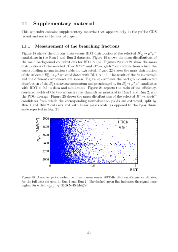
Supplementary material full pdf