Observation of the $B^0\rightarrow\overline{D}^{*0}K^{+}\pi^{-}$ and $B_s^0\rightarrow\overline{D}^{*0}K^{-}\pi^{+}$ decays
[to restricted-access page]Information
LHCb-PAPER-2021-043
CERN-EP-2021-262
arXiv:2112.11428 [PDF]
(Submitted on 21 Dec 2021)
Phys. Rev. D105 (2022) 072005
Inspire 1994799
Tools
Abstract
The first observations of $B^0\rightarrow\overline{D}^{*}(2007)^{0}K^{+}\pi^{-}$ and $B_s^0\rightarrow\overline{D}^{*}(2007)^{0}K^{-}\pi^{+}$ decays are presented, and their branching fractions relative to that of the $B^0\rightarrow\overline{D}^{*}(2007)^{0}\pi^{+}\pi^{-}$ decay are reported. These modes can potentially be used to investigate the spectroscopy of charm and charm-strange resonances and to determine the angle $\gamma$ of the CKM unitarity triangle. It is also important to understand them as a source of potential background in determinations of $\gamma$ from $B^{+}\rightarrow DK^{+}$ and $B^{0}\rightarrow DK^{+}\pi^{-}$ decays. The analysis is based on a sample corresponding to an integrated luminosity of $5.4 \rm{fb}^{-1}$ of proton--proton collision data at $13 \rm{TeV}$ centre-of-mass energy recorded with the LHCb detector. The $\overline{D}^{*}(2007)^{0}$ mesons are fully reconstructed in the $\overline{D}^{0}\pi^{0}$ and $\overline{D}^{0}\gamma$ channels, with the $\overline{D}^{0} \rightarrow K^{+}\pi^{-}$ decay. A novel weighting method is used to subtract background while simultaneously applying an event-by-event efficiency correction to account for resonant structures in the decays.
Figures and captions
|
Leading diagrams for ($a$), ($c$) $ B ^0 \rightarrow \overline{ D }{} {}^{*0} K ^+ \pi ^- $ and ($b$), ($d$) $ B ^0_ s \rightarrow \overline{ D }{} {}^{*0} K ^- \pi ^+ $ decay channels. In the colour-suppressed diagrams, ($a$) and ($b$), the decay proceeds through an intermediate $\optbar{ K}{} {}^{*0}$ resonance with additional $ u \overline u $ production, while in the colour-allowed diagrams the decay proceeds through an excited charm ($c$) or charm-strange ($d$) resonance. |
figure[..].pdf [62 KiB] HiDef png [30 KiB] Thumbnail [15 KiB] *.C file |

|
|
figure[..].pdf [62 KiB] HiDef png [28 KiB] Thumbnail [14 KiB] *.C file |

|
|
|
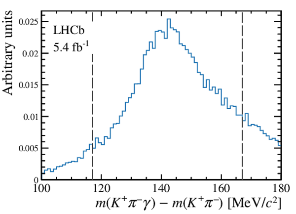
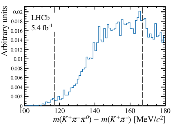
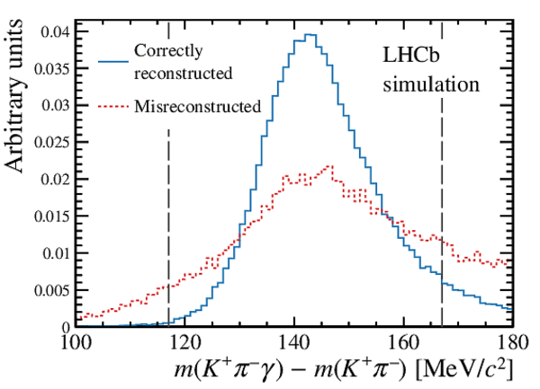
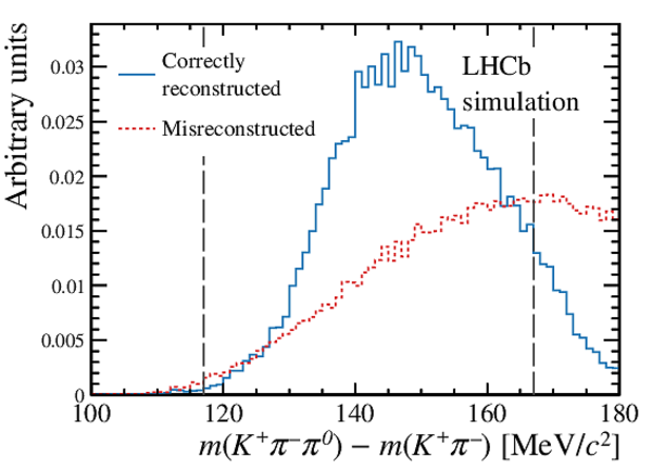
Difference between the $\overline{ D }{} {}^{*0}$ and $\overline{ D }{} {}^0$ candidate masses in $ B ^0 \rightarrow \overline{ D }{} {}^{*0} \pi ^+ \pi ^- $ decays for (top) data and (bottom) simulated signal decays. The left and right plots show $\overline{ D }{} {}^{*0} \rightarrow \overline{ D }{} {}^0 \gamma$ and $\overline{ D }{} {}^0 \pi ^0 $ candidates, respectively. The simulation distributions are shown separately for correctly reconstructed and misreconstructed signal components. All selection requirements have been imposed, except those on the plotted variable, which are indicated with dashed vertical lines. |
Data_C[..].pdf [14 KiB] HiDef png [144 KiB] Thumbnail [133 KiB] *.C file |
|
|
Data_C[..].pdf [14 KiB] HiDef png [165 KiB] Thumbnail [157 KiB] *.C file |
|
|
|
MC_Cog[..].pdf [15 KiB] HiDef png [222 KiB] Thumbnail [196 KiB] *.C file |
|
|
|
MC_Cop[..].pdf [15 KiB] HiDef png [210 KiB] Thumbnail [182 KiB] *.C file |
|
|
|
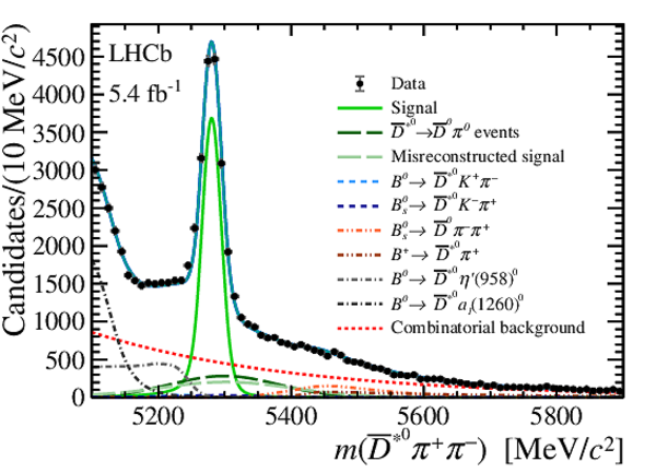
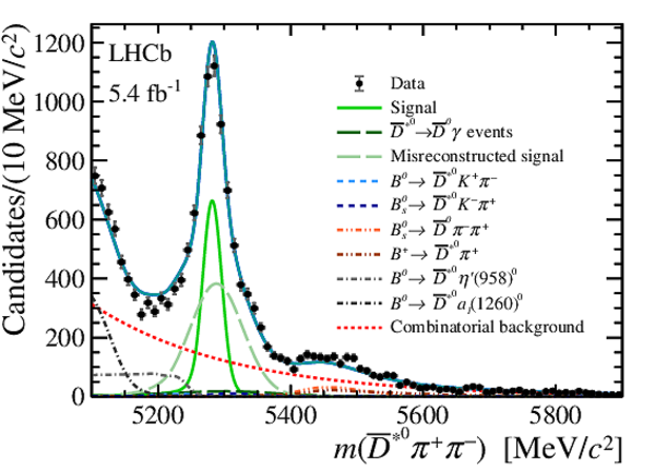
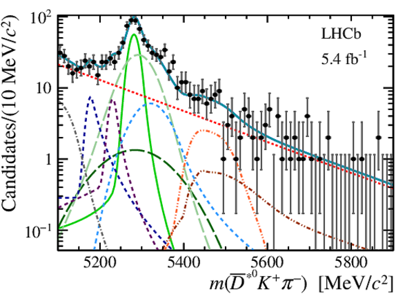
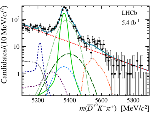
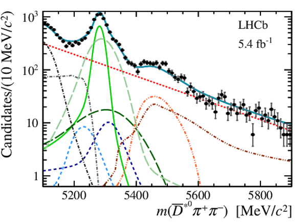
Invariant mass distributions of (top) $B^0\rightarrow \overline{ D }{} {}^{*0} K ^+ \pi ^- $, (middle) $ B ^0_ s \rightarrow \overline{ D }{} {}^{*0} K ^- \pi ^+ $, and (bottom) $B^0\rightarrow \overline{ D }{} {}^{*0} \pi ^+ \pi ^- $ with (left) $\overline{ D }{} {}^{*0} \rightarrow \overline{ D }{} {}^0 \gamma$ and (right) $\overline{ D }{} {}^{*0} \rightarrow \overline{ D }{} {}^0 \pi ^0 $ candidates, with linear $y$-axis. The total fit result is shown overlaid as a solid blue line, with individual components illustrated as indicated in the legends. |
B0g_Fu[..].pdf [36 KiB] HiDef png [432 KiB] Thumbnail [310 KiB] *.C file |

|
|
B0p_Fu[..].pdf [34 KiB] HiDef png [413 KiB] Thumbnail [298 KiB] *.C file |

|
|
|
Bsg_Fu[..].pdf [35 KiB] HiDef png [392 KiB] Thumbnail [276 KiB] *.C file |

|
|
|
Bsp_Fu[..].pdf [35 KiB] HiDef png [392 KiB] Thumbnail [284 KiB] *.C file |

|
|
|
Cog_Fu[..].pdf [37 KiB] HiDef png [439 KiB] Thumbnail [325 KiB] *.C file |
|
|
|
Cop_Fu[..].pdf [36 KiB] HiDef png [415 KiB] Thumbnail [298 KiB] *.C file |
|
|
|
Invariant mass distributions of (top) $B^0\rightarrow \overline{ D }{} {}^{*0} K ^+ \pi ^- $, (middle) $ B ^0_ s \rightarrow \overline{ D }{} {}^{*0} K ^- \pi ^+ $, and (bottom) $B^0\rightarrow \overline{ D }{} {}^{*0} \pi ^+ \pi ^- $ with (left) $\overline{ D }{} {}^{*0} \rightarrow \overline{ D }{} {}^0 \gamma$ and (right) $\overline{ D }{} {}^{*0} \rightarrow \overline{ D }{} {}^0 \pi ^0 $ candidates, with logarithmic $y$-axis scale. The total fit result is shown overlaid as a solid blue line, with individual components illustrated as indicated in the legends of \cref{fig:globalfit_lin}. |
B0g_Fu[..].pdf [34 KiB] HiDef png [456 KiB] Thumbnail [302 KiB] *.C file |

|
|
B0p_Fu[..].pdf [32 KiB] HiDef png [488 KiB] Thumbnail [315 KiB] *.C file |
|
|
|
Bsg_Fu[..].pdf [33 KiB] HiDef png [409 KiB] Thumbnail [269 KiB] *.C file |

|
|
|
Bsp_Fu[..].pdf [32 KiB] HiDef png [422 KiB] Thumbnail [280 KiB] *.C file |
|
|
|
Cog_Fu[..].pdf [34 KiB] HiDef png [391 KiB] Thumbnail [267 KiB] *.C file |

|
|
|
Cop_Fu[..].pdf [34 KiB] HiDef png [424 KiB] Thumbnail [287 KiB] *.C file |
|
|
|
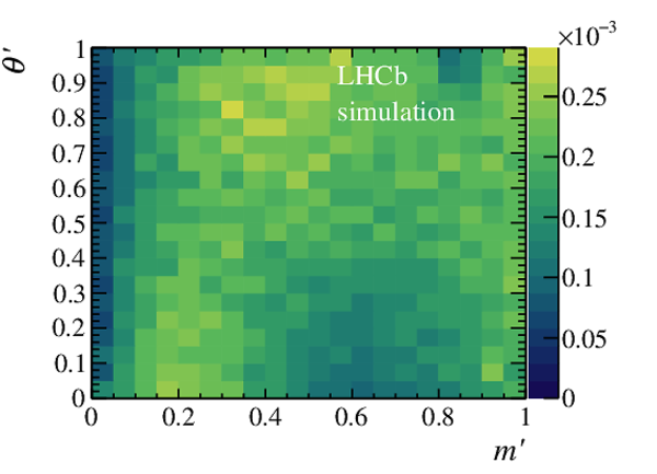
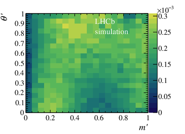
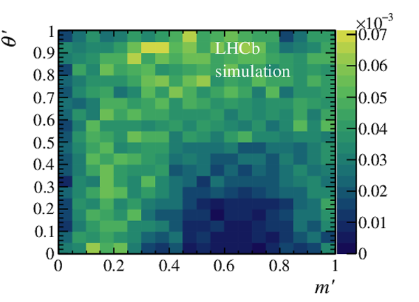
Total efficiency as a function of SDP coordinates for (top) $ B ^0 \rightarrow \overline{ D }{} {}^{*0} K ^+ \pi ^- $, (middle) $ B ^0_ s \rightarrow \overline{ D }{} {}^{*0} K ^- \pi ^+ $, and (bottom) $ B ^0 \rightarrow \overline{ D }{} {}^{*0} \pi ^+ \pi ^- $, with (left) $\overline{ D }{} {}^{*0} \rightarrow \overline{ D }{} {}^0 \gamma$ and (right) $\overline{ D }{} {}^{*0} \rightarrow \overline{ D }{} {}^0 \pi ^0 $ decays. |
B0g_MCEff.pdf [16 KiB] HiDef png [228 KiB] Thumbnail [198 KiB] *.C file |
|
|
B0p_MCEff.pdf [16 KiB] HiDef png [241 KiB] Thumbnail [208 KiB] *.C file |

|
|
|
Bsg_MCEff.pdf [16 KiB] HiDef png [231 KiB] Thumbnail [201 KiB] *.C file |
|
|
|
Bsp_MCEff.pdf [16 KiB] HiDef png [245 KiB] Thumbnail [205 KiB] *.C file |
|
|
|
Cog_MCEff.pdf [16 KiB] HiDef png [235 KiB] Thumbnail [199 KiB] *.C file |

|
|
|
Cop_MCEff.pdf [16 KiB] HiDef png [227 KiB] Thumbnail [195 KiB] *.C file |

|
|
|
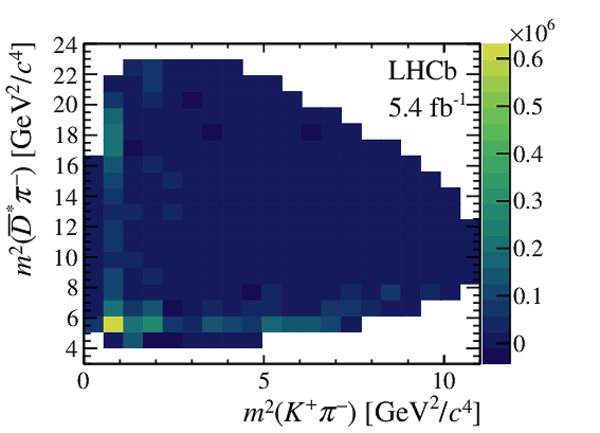
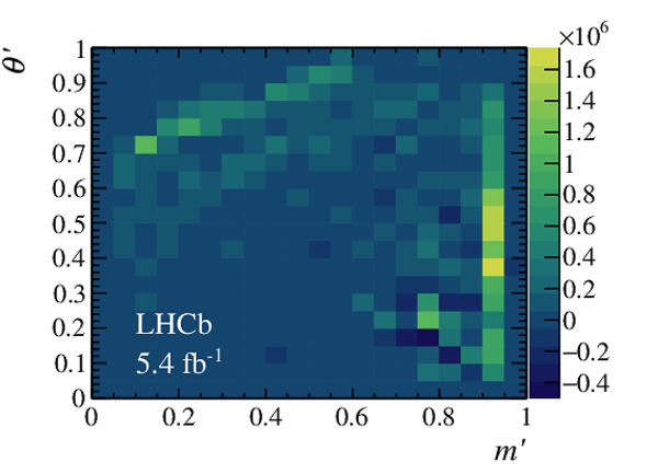
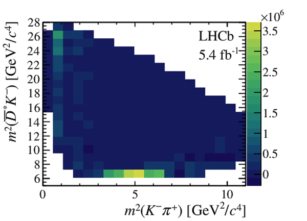
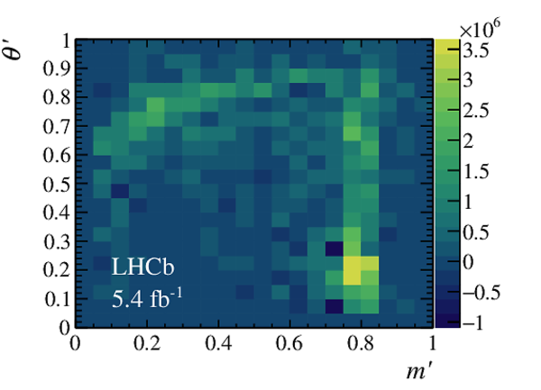
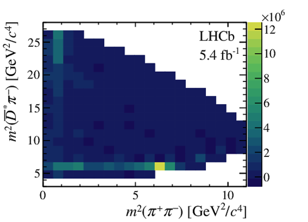
(Left) SDP and (right) conventional Dalitz plots of background-subtracted and efficiency-corrected data, for (top) $ B ^0 \rightarrow \overline{ D }{} {}^{*0} K ^+ \pi ^- $, (middle) $ B ^0_ s \rightarrow \overline{ D }{} {}^{*0} K ^- \pi ^+ $ and (bottom) $ B ^0 \rightarrow \overline{ D }{} {}^{*0} \pi ^+ \pi ^- $ decays. |
B0g_SQ[..].pdf [16 KiB] HiDef png [195 KiB] Thumbnail [185 KiB] *.C file |

|
|
B0g_Da[..].pdf [15 KiB] HiDef png [155 KiB] Thumbnail [172 KiB] *.C file |
|
|
|
Bsg_SQ[..].pdf [16 KiB] HiDef png [198 KiB] Thumbnail [195 KiB] *.C file |
|
|
|
Bsg_Da[..].pdf [15 KiB] HiDef png [156 KiB] Thumbnail [174 KiB] *.C file |
|
|
|
Cog_SQ[..].pdf [16 KiB] HiDef png [203 KiB] Thumbnail [191 KiB] *.C file |
|
|
|
Cog_Da[..].pdf [15 KiB] HiDef png [135 KiB] Thumbnail [145 KiB] *.C file |
|
|
|
Animated gif made out of all figures. |
PAPER-2021-043.gif Thumbnail |

|
![HiDef png [30 KiB]](Directory_LHCb-PAPER-2021-043/hidef_figure_diagrams1.png)
![HiDef png [28 KiB]](Directory_LHCb-PAPER-2021-043/hidef_figure_diagrams2.png)
![HiDef png [144 KiB]](Directory_LHCb-PAPER-2021-043/hidef_Data_Cog_DstCut.png)
![HiDef png [165 KiB]](Directory_LHCb-PAPER-2021-043/hidef_Data_Cop_DstCut.png)
![HiDef png [222 KiB]](Directory_LHCb-PAPER-2021-043/hidef_MC_Cog_DstCut.png)
![HiDef png [210 KiB]](Directory_LHCb-PAPER-2021-043/hidef_MC_Cop_DstCut.png)
![HiDef png [432 KiB]](Directory_LHCb-PAPER-2021-043/hidef_B0g_FullFit_NoPull.png)
![HiDef png [413 KiB]](Directory_LHCb-PAPER-2021-043/hidef_B0p_FullFit_NoPull.png)
![HiDef png [392 KiB]](Directory_LHCb-PAPER-2021-043/hidef_Bsg_FullFit_NoPull.png)
![HiDef png [392 KiB]](Directory_LHCb-PAPER-2021-043/hidef_Bsp_FullFit_NoPull.png)
![HiDef png [439 KiB]](Directory_LHCb-PAPER-2021-043/hidef_Cog_FullFit_NoPull.png)
![HiDef png [415 KiB]](Directory_LHCb-PAPER-2021-043/hidef_Cop_FullFit_NoPull.png)
![HiDef png [456 KiB]](Directory_LHCb-PAPER-2021-043/hidef_B0g_FullFit_NoPull_log.png)
![HiDef png [488 KiB]](Directory_LHCb-PAPER-2021-043/hidef_B0p_FullFit_NoPull_log.png)
![HiDef png [409 KiB]](Directory_LHCb-PAPER-2021-043/hidef_Bsg_FullFit_NoPull_log.png)
![HiDef png [422 KiB]](Directory_LHCb-PAPER-2021-043/hidef_Bsp_FullFit_NoPull_log.png)
![HiDef png [391 KiB]](Directory_LHCb-PAPER-2021-043/hidef_Cog_FullFit_NoPull_log.png)
![HiDef png [424 KiB]](Directory_LHCb-PAPER-2021-043/hidef_Cop_FullFit_NoPull_log.png)
![HiDef png [228 KiB]](Directory_LHCb-PAPER-2021-043/hidef_B0g_MCEff.png)
![HiDef png [241 KiB]](Directory_LHCb-PAPER-2021-043/hidef_B0p_MCEff.png)
![HiDef png [231 KiB]](Directory_LHCb-PAPER-2021-043/hidef_Bsg_MCEff.png)
![HiDef png [245 KiB]](Directory_LHCb-PAPER-2021-043/hidef_Bsp_MCEff.png)
![HiDef png [235 KiB]](Directory_LHCb-PAPER-2021-043/hidef_Cog_MCEff.png)
![HiDef png [227 KiB]](Directory_LHCb-PAPER-2021-043/hidef_Cop_MCEff.png)
![HiDef png [195 KiB]](Directory_LHCb-PAPER-2021-043/hidef_B0g_SQD_EffCorr.png)
![HiDef png [155 KiB]](Directory_LHCb-PAPER-2021-043/hidef_B0g_Dalitz_EffCorr.png)
![HiDef png [198 KiB]](Directory_LHCb-PAPER-2021-043/hidef_Bsg_SQD_EffCorr.png)
![HiDef png [156 KiB]](Directory_LHCb-PAPER-2021-043/hidef_Bsg_Dalitz_EffCorr.png)
![HiDef png [203 KiB]](Directory_LHCb-PAPER-2021-043/hidef_Cog_SQD_EffCorr.png)
![HiDef png [135 KiB]](Directory_LHCb-PAPER-2021-043/hidef_Cog_Dalitz_EffCorr.png)
Tables and captions
|
Yields obtained from the simultaneous fit for the correctly reconstructed signal component. Uncertainties are statistical only. |
Table_1.pdf [67 KiB] HiDef png [91 KiB] Thumbnail [47 KiB] tex code |

|
|
Correlations between the signal yields, as obtained from the simultaneous fit, accounting for statistical uncertainties only. The individual components are labelled with a shorthand, following the same ordering (left to right, and top to bottom) as in \cref{tab:FitResults}. The symbols $\overline{ D }{} {}^{*0}_{\gamma}$ and $\overline{ D }{} {}^{*0}_{\pi ^0 }$ refer to $\overline{ D }{} {}^{*0} \rightarrow \overline{ D }{} {}^0 \gamma$ and $\overline{ D }{} {}^{*0} \rightarrow \overline{ D }{} {}^0 \pi ^0 $ decays, respectively. |
Table_2.pdf [71 KiB] HiDef png [47 KiB] Thumbnail [21 KiB] tex code |

|
|
Ordering convention used to define the SDP representation of the phase space for each of the signal decays. |
Table_3.pdf [64 KiB] HiDef png [52 KiB] Thumbnail [24 KiB] tex code |

|
|
Systematic uncertainties (%) on the branching fraction ratios, relative to the central values, with the soft neutral particle emitted in the $\overline{ D }{} {}^{*0}$ decay indicated as a subscript for brevity of notation. The sources of uncertainty are presented in the same order as described in the text, with statistical uncertainties included to facilitate comparison. Systematic uncertainties are indicated as being considered to be either completely uncorrelated ($\dagger$) or completely correlated ($*$) between the ratios obtained with the $\overline{ D }{} {}^{*0} \rightarrow \overline{ D }{} {}^0 \gamma$ and $\overline{ D }{} {}^{*0} \rightarrow \overline{ D }{} {}^0 \pi ^0 $ decays. The total correlated and uncorrelated systematic uncertainties are obtained by summing the relevant sources in quadrature. The uncertainty due to the fragmentation fractions is quoted separately. |
Table_4.pdf [87 KiB] HiDef png [62 KiB] Thumbnail [30 KiB] tex code |

|
|
Branching fraction ratios determined separately for $\overline{ D }{} {}^{*0} \rightarrow \overline{ D }{} {}^0 \gamma$ and $\overline{ D }{} {}^{*0} \rightarrow \overline{ D }{} {}^0 \pi ^0 $ decays. The uncertainties are statistical, systematic and (where given) due to $f_s/f_d$. |
Table_5.pdf [88 KiB] HiDef png [48 KiB] Thumbnail [22 KiB] tex code |

|
![HiDef png [91 KiB]](Directory_LHCb-PAPER-2021-043/hidef_Table_1.png)
![HiDef png [47 KiB]](Directory_LHCb-PAPER-2021-043/hidef_Table_2.png)
![HiDef png [52 KiB]](Directory_LHCb-PAPER-2021-043/hidef_Table_3.png)
![HiDef png [62 KiB]](Directory_LHCb-PAPER-2021-043/hidef_Table_4.png)
![HiDef png [48 KiB]](Directory_LHCb-PAPER-2021-043/hidef_Table_5.png)
Created on 02 May 2024.