Search for rare decays of $D^0$ mesons into two muons

Information

LHCb-PAPER-2022-029
CERN-EP-2022-273
arXiv:2212.11203 [PDF]

(Submitted on 21 Dec 2022)
Phys. Rev. Lett. 131 (2023) 041804
Inspire 2681870

Tools

Abstract

A search for the very rare $D^0 \to \mu^+\mu^-$ decay is performed using data collected by the LHCb experiment in proton-proton collisions at $\sqrt{s} = 7$, 8 and $13 \rm{TeV}$, corresponding to an integrated luminosity of $9 \rm{fb^{-1}}$. The search is optimised for $D^0$ mesons from $D^{\ast+}\to D^0\pi^+$ decays but is also sensitive to $D^0$ mesons from other sources. No evidence for an excess of events over the expected background is observed. An upper limit on the branching fraction of this decay is set at $\mathcal{B}(D^0 \to \mu^+\mu^-) < 3.1 \times 10^{-9}$ at a $90\%$ CL. This represents the world's most stringent limit, constraining models of physics beyond the Standard Model.

Figures and captions

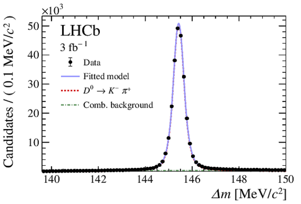
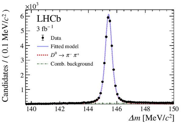
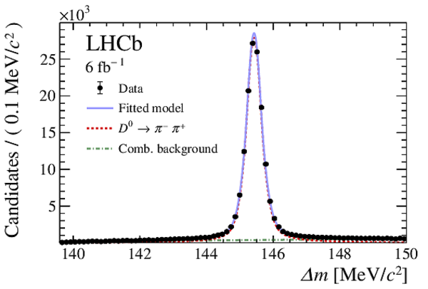
Distributions of $\Delta m$ for (left) $ D ^0 \rightarrow K ^- \pi ^+ $ and (right) $ D ^0 \rightarrow \pi ^+ \pi ^- $ normalisation channels candidates for (top) Run 1 and (bottom) Run 2 data. The distributions are superimposed with the fit.	Fig1a.pdf [32 KiB] HiDef png [192 KiB] Thumbnail [154 KiB]
	Fig1b.pdf [32 KiB] HiDef png [195 KiB] Thumbnail [154 KiB]
	Fig1c.pdf [32 KiB] HiDef png [208 KiB] Thumbnail [168 KiB]
	Fig1d.pdf [32 KiB] HiDef png [205 KiB] Thumbnail [158 KiB]
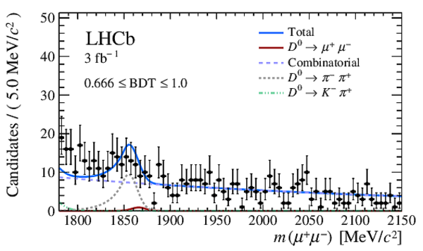
Distribution of (left) $ m(\mu ^+\mu ^- )$ and (right) $\Delta m$ for the $ D ^0 \rightarrow \mu ^+ \mu ^- $ candidates in data from (top) Run 1 and (bottom) Run 2 , for the most sensitive BDT interval. The distribution is superimposed with the fit to data. Each of the two distributions is in the signal region of the other variable, see text for details. Untagged and tagged decays are included in a single component for signal and $ D ^0 \rightarrow \pi ^+ \pi ^- $ background.	Fig2a.pdf [31 KiB] HiDef png [276 KiB] Thumbnail [223 KiB]
	Fig2b.pdf [29 KiB] HiDef png [257 KiB] Thumbnail [199 KiB]
	Fig2c.pdf [33 KiB] HiDef png [291 KiB] Thumbnail [238 KiB]
	Fig2d.pdf [30 KiB] HiDef png [254 KiB] Thumbnail [194 KiB]
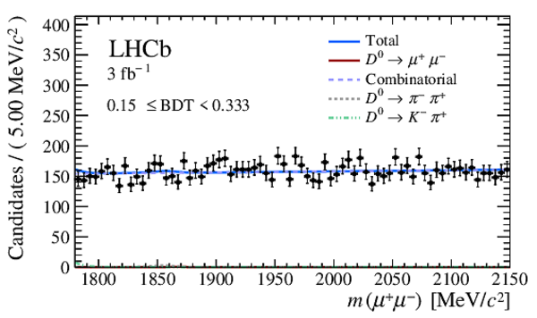
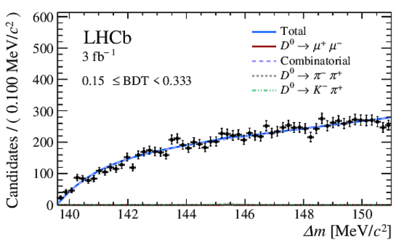
Distributions of (left) $ m(\mu ^+\mu ^- )$ and (right) $\Delta m$ for the $ D ^0 \rightarrow \mu ^+ \mu ^- $ candidates for Run 1 data in, top to bottom, the three BDT intervals. The distributions are superimposed with the fit to data. Each of the two distributions is in the signal region of the other variable, see text for details. Untagged and tagged decays are included in a single component for signal and $ D ^0 \rightarrow \pi ^+ \pi ^- $ background.	Fig3a.pdf [31 KiB] HiDef png [268 KiB] Thumbnail [229 KiB]
	Fig3b.pdf [28 KiB] HiDef png [236 KiB] Thumbnail [188 KiB]
	Fig3c.pdf [31 KiB] HiDef png [278 KiB] Thumbnail [229 KiB]
	Fig3d.pdf [29 KiB] HiDef png [244 KiB] Thumbnail [192 KiB]
	Fig3e.pdf [31 KiB] HiDef png [276 KiB] Thumbnail [223 KiB]
	Fig3f.pdf [29 KiB] HiDef png [257 KiB] Thumbnail [199 KiB]
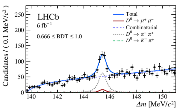
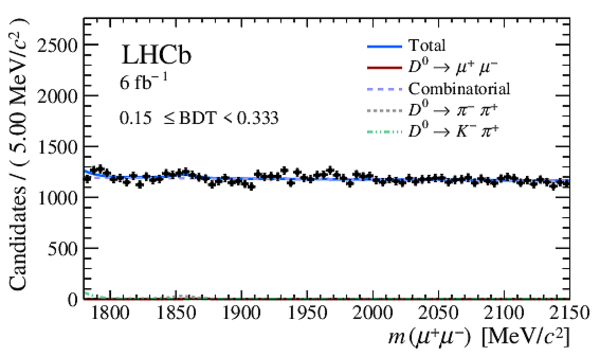
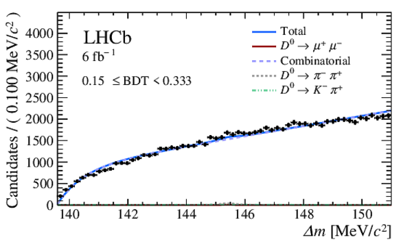
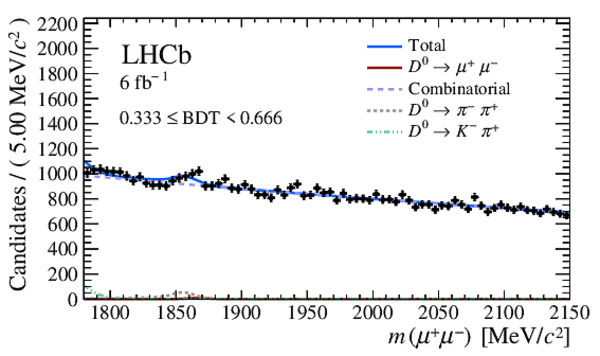
Distributions of (left) $ m(\mu ^+\mu ^- )$ and (right) $\Delta m$ for the $ D ^0 \rightarrow \mu ^+ \mu ^- $ candidates for Run 2 data in, top to bottom, the three BDT bins. The distributions are superimposed with the fit to data. Each of the two distributions is in the signal region of the other variable, see text for details. Untagged and tagged decays are included in a single component for signal and $ D ^0 \rightarrow \pi ^+ \pi ^- $ background.	Fig4a.pdf [32 KiB] HiDef png [269 KiB] Thumbnail [224 KiB]
	Fig4b.pdf [29 KiB] HiDef png [241 KiB] Thumbnail [188 KiB]
	Fig4c.pdf [32 KiB] HiDef png [277 KiB] Thumbnail [227 KiB]
	Fig4d.pdf [29 KiB] HiDef png [245 KiB] Thumbnail [189 KiB]
	Fig4e.pdf [33 KiB] HiDef png [291 KiB] Thumbnail [238 KiB]
	Fig4f.pdf [30 KiB] HiDef png [254 KiB] Thumbnail [194 KiB]
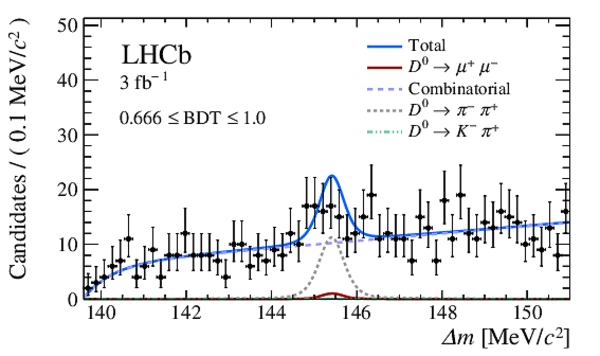
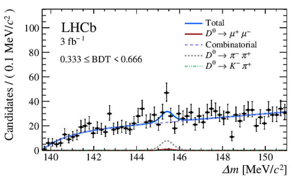
Distributions of (left) $ m(\mu ^+\mu ^- )$ and (right) $\Delta m$ for the $ D ^0 \rightarrow \mu ^+ \mu ^- $ candidates for Run 1 data in, top to bottom, the three BDT bins. The distributions are superimposed with the fit to data. Untagged and tagged decays are included in a single component for signal and $ D ^0 \rightarrow \pi ^+ \pi ^- $ background. Unlike the correspondent figures in the main body of the Letter, here all events are shown.	Fig5a.pdf [31 KiB] HiDef png [268 KiB] Thumbnail [226 KiB]
	Fig5b.pdf [29 KiB] HiDef png [237 KiB] Thumbnail [187 KiB]
	Fig5c.pdf [32 KiB] HiDef png [271 KiB] Thumbnail [224 KiB]
	Fig5d.pdf [29 KiB] HiDef png [237 KiB] Thumbnail [186 KiB]
	Fig5e.pdf [32 KiB] HiDef png [283 KiB] Thumbnail [239 KiB]
	Fig5f.pdf [29 KiB] HiDef png [244 KiB] Thumbnail [191 KiB]
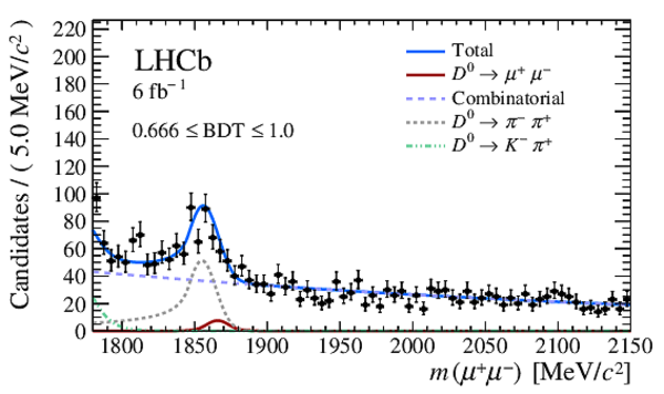
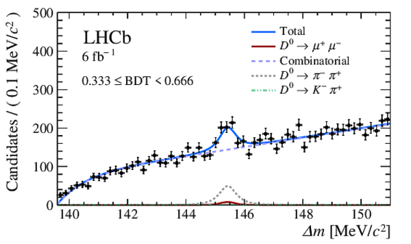
Distributions of (left) $ m(\mu ^+\mu ^- )$ and (right) $\Delta m$ for the $ D ^0 \rightarrow \mu ^+ \mu ^- $ candidates for Run 2 data in, top to bottom, the three BDT bins. The distributions are superimposed with the fit to data. Untagged and tagged decays are included in a single component for signal and $ D ^0 \rightarrow \pi ^+ \pi ^- $ background. Unlike the correspondent figures in the main body of the Letter, here all events are shown.	Fig6a.pdf [31 KiB] HiDef png [243 KiB] Thumbnail [193 KiB]
	Fig6b.pdf [29 KiB] HiDef png [236 KiB] Thumbnail [187 KiB]
	Fig6c.pdf [32 KiB] HiDef png [274 KiB] Thumbnail [222 KiB]
	Fig6d.pdf [30 KiB] HiDef png [231 KiB] Thumbnail [180 KiB]
	Fig6e.pdf [32 KiB] HiDef png [256 KiB] Thumbnail [198 KiB]
	Fig6f.pdf [29 KiB] HiDef png [242 KiB] Thumbnail [181 KiB]
Two-dimensional distribution of $ m( D ^0 )$ versus $\Delta m$ for the most sensitive BDT interval in the (left) Run 1 and (right) Run 2 data. Red lines represent the signal region of each variable as defined in the text.	Fig7a.pdf [60 KiB] HiDef png [330 KiB] Thumbnail [387 KiB]
	Fig7b.pdf [245 KiB] HiDef png [886 KiB] Thumbnail [739 KiB]
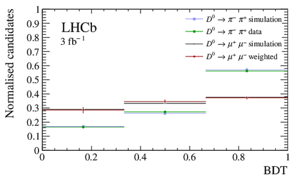
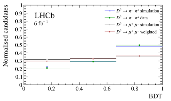
Distribution of the BDT output. The $ D ^0 \rightarrow \pi ^+ \pi ^- $ candidates in data and simulation are shown and used to weight the simulated $ D ^0 \rightarrow \mu ^+ \mu ^- $ decays distribution used for the search.	Fig8a.pdf [15 KiB] HiDef png [130 KiB] Thumbnail [127 KiB]
	Fig8b.pdf [15 KiB] HiDef png [129 KiB] Thumbnail [126 KiB]
Efficiency for two pions to pass a requirement on the $ProbNNmu$ variable (after additional requirements on its identification as muon) in Run 2, as measured from $ D ^+ \rightarrow \pi ^+ \pi ^- \pi ^+ $ and $ D ^+_ s \rightarrow \pi ^+ \pi ^- \pi ^+ $ decays in data and $ D ^0 \rightarrow \pi ^+ \pi ^- $ decays in simulation. Same sign pions are used in data to avoid contamination for hadronic resonances decaying to two real muons.	Fig9.pdf [17 KiB] HiDef png [223 KiB] Thumbnail [189 KiB]
Value of $\rm{CL_s}$ as a function of the $ D ^0 \rightarrow \mu ^+ \mu ^- $ branching fraction.	Fig10.pdf [14 KiB] HiDef png [307 KiB] Thumbnail [201 KiB]
Animated gif made out of all figures.	PAPER-2022-029.gif Thumbnail