Leading-order Feynman diagrams for $ b \rightarrow s \ell^+ \ell^-$ transitions in the SM.

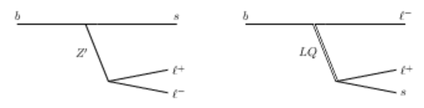
Examples of Feynman diagrams for $ b \rightarrow s \ell^+ \ell^-$ decays beyond the SM. Potential contributions from new heavy $Z^\prime$ gauge bosons are shown on the left, contributions from leptoquarks (LQ) on the right.

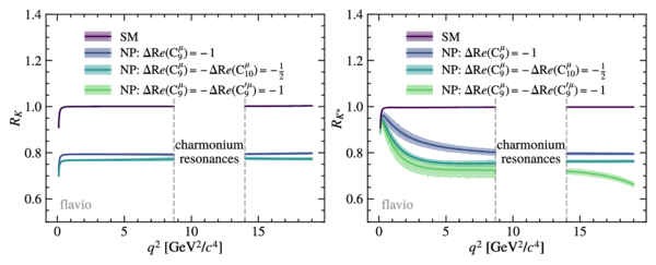
Variation of (left) $ R_K$ and (right) $ R_{ K ^* }$ as a function of $ q^2$ within the SM obtained using the \texttt{flavio} software package [71], taking into account potential heavy BSM contributions to the Wilson coefficients. The contributions from $ c \overline c $ resonances are subtracted in both cases. For $ R_K$ , the SM prediction overlaps with the BSM scenario $\Delta {\cal R}e(C_9^\mu)=-\Delta {\cal R}e(C_9^{\prime\mu})=-1$.

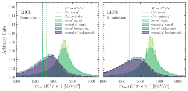
Distribution of $ m_{\mathrm{corr}}$ for the simulated (left) $ B ^+ \rightarrow K ^+ e ^+ e ^- $ and (right) $ B ^0 \rightarrow K ^{*0} e ^+ e ^- $ candidates after applying the nominal analysis criteria to the response of the combinatorial and partially reconstructed multivariate classifiers. The distributions of the signal in the low- and $\text{central-} q^2 $ regions and the partially reconstructed background are shown (unit normalizations). The $ B ^+$ and $ B ^0$ partially reconstructed backgrounds are taken from simulated $ B ^0 \rightarrow K ^{*0} e ^+ e ^- $ and $ B ^+ \rightarrow K ^+ \pi ^+ \pi ^- e ^+ e ^- $ decays, respectively. The vertical lines show the selection requirements applied for the two signal regions.

Simulated distributions of (left) $m( K ^+ e ^- )$ for $ B ^+ $ candidates and (right) $m( K ^+ \pi ^- e ^- )$ for $ B ^0$ candidates. Signal and various semileptonic cascade backgrounds are shown. The full selection is applied except for the semileptonic background vetos. The hatched areas show decay modes that are also vetoed, recomputing $m( K ^+ e ^- )$ and $m( K ^+ \pi ^- e ^- )$ while assigning the pion mass hypothesis to the electron and not accounting for bremsstrahlung corrections.

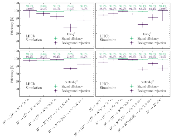
Upper: signal efficiencies and background rejection factors for all vetos against physical backgrounds, for (left) $ B ^+ $ and (right) $ B ^0$ modes, in the $\text{low-} q^2 $ region; lower: analogous plots for the $\text{central-} q^2 $ region.

Distributions of the invariant mass of candidates for which both electrons are in the control region, i.e. having the stringent electron identification requirements inverted. The pion mass hypothesis is applied to both electrons, without a bremsstrahlung correction. The left and right columns correspond to the $ B ^+ \rightarrow K ^+ e ^+ e ^- $ and $ B ^0 \rightarrow K ^{*0} e ^+ e ^- $ modes, respectively. The upper and lower rows correspond to the low- and $\text{central-} q^2 $ regions, respectively. Fit results are overlaid.

Distributions of the invariant mass of candidates for which both electrons are in the control region, i.e. having the stringent electron identification requirements inverted. The kaon mass hypothesis is applied to both electrons, without a bremsstrahlung correction. Fit results are overlaid. (left) $ B ^+ \rightarrow K ^+ e ^+ e ^- $ modes, (right) $ B ^0 \rightarrow K ^{*0} e ^+ e ^- $ modes. The upper and lower rows correspond to the low- and $\text{central-} q^2 $ regions, respectively.

Invariant mass distribution of candidates in the inverted lepton identification control region. From top to bottom: $ R_K$ $\text{low-} q^2 $ , $ R_K$ $\text{central-} q^2 $ , $ R_{ K ^* }$ $\text{low-} q^2 $ , $ R_{ K ^* }$ $\text{central-} q^2 $ . (Left) candidates for which the lepton is in the control region and has the same charge as the kaon, (middle) candidates for which the lepton is in the control region and has a charge which is the opposite of that of the kaon, (right) candidates for which both leptons are in the control region.

Upper: distributions of the PID variables in the (left) pion and (right) kaon calibration samples using 2017 data. The red lines separate control regions (left and below the line) from fit regions (right and above the line). Lower: the fraction of control region events that is expected to appear in the fit region (transfer function) as functions of track $ p_{\mathrm{T}}$ and $\eta$.

Distributions of misidentified background events predicted for the $ K ^+ e ^+ e ^- $ and $ K ^{*0} e ^+ e ^- $ samples with full selection criteria applied.

Factorization bias as a function of the separation between a pair of electrons in the electromagnetic calorimeter in the various $q^{2}$ regions determined using simulated $B^{+}\rightarrow K^{+}e^{+}e^{-}$ decays.

Distributions of selected measured quantities for \textrm{TOS} $ B ^+ \rightarrow K ^+ { J \mskip -3mu/\mskip -2mu\psi } ( e ^+ e ^- )$ candidates in the 2016 data, compared with simulation before (red) and after (blue) calibrations.

Distributions of the dielectron invariant mass for $ B ^+ \rightarrow K ^+ { J \mskip -3mu/\mskip -2mu\psi } ( e ^+ e ^- )$ candidates in (left) simulation and (right) data, for each of the three bremsstrahlung categories (from top to bottom), overlaid with the projections of the fit model. The candidates correspond to the 2018 data and the TIS trigger category.

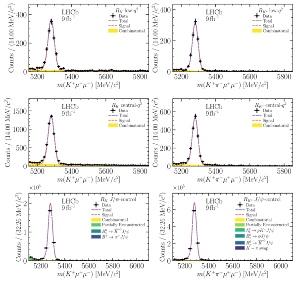
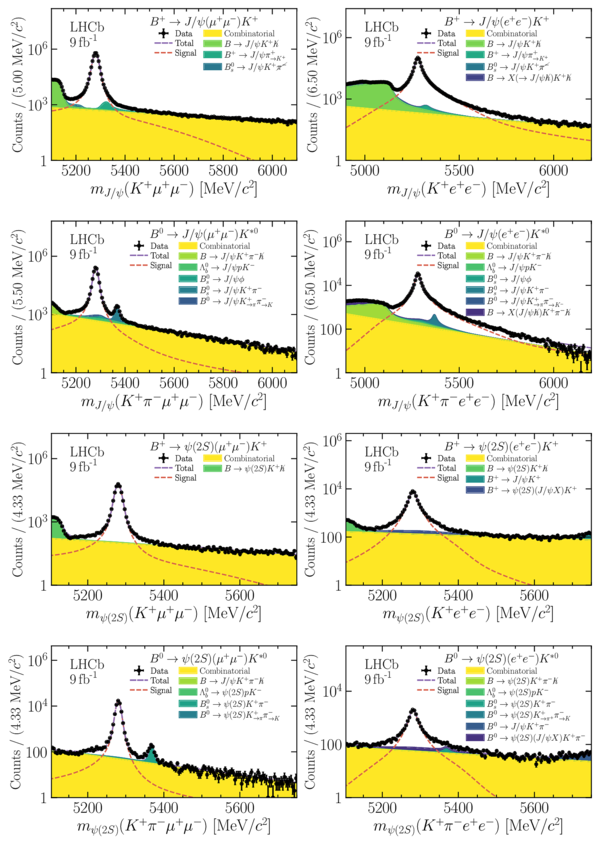
Distributions of (left) $m(K^{+}\mu^{+}\mu^{-})$ and (right) $m(K^{+}\pi^{-}\mu^{+}\mu^{-})$ of $\text{low-} q^2 $ , $\text{central-} q^2 $ , and $ { J \mskip -3mu/\mskip -2mu\psi }$ -control regions (from top to bottom), overlaid with the projections of the fit model. Each of the fit components are discussed in Section 7.1.

Distributions of (left) $m(K^{+}e^{+}e^{-})$ and (right) $m(K^{+}\pi^{-}e^{+}e^{-})$ in the (top to bottom) $\text{low-} q^2 $ , $\text{central-} q^2 $ , and $ { J \mskip -3mu/\mskip -2mu\psi }$ -control regions, overlaid with the projections of the fit model. Each of the fit components are discussed in Sec. 7.1.

Template shapes for misidentified backgrounds obtained from data. The shapes for Run 1 are given on the left, the shapes for Run 2 are given on the right. From top to bottom, the shapes for $ R_K$ in $\text{low-} q^2 $ , $ R_K$ in $\text{central-} q^2 $ , $ R_{ K ^* }$ in $\text{low-} q^2 $ and $ R_{ K ^* }$ in $\text{central-} q^2 $ regions are given.

Invariant mass fit to the resonant control modes, from top to bottom: $ { J \mskip -3mu/\mskip -2mu\psi }$ mode in $ B ^+ \rightarrow K ^+ \ell^+ \ell^- $ , $ { J \mskip -3mu/\mskip -2mu\psi }$ mode in $ B ^0 \rightarrow K ^{*0} \ell^+ \ell^- $ , $\psi {(2S)}$ mode in $ B ^+ \rightarrow K ^+ \ell^+ \ell^- $ , $\psi {(2S)}$ in $ B ^0 \rightarrow K ^{*0} \ell^+ \ell^- $ . The muon (electron) modes are given on the left (right).

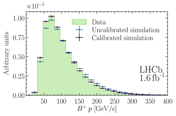
Evolution of the $ r_{ { J \mskip -3mu/\mskip -2mu\psi } }^{ K }$ single and $ R_{\psi {(2S)} }^{ K }$ double ratios with each step of the simulation calibration procedure as labeled on the $x$-axis. The data-taking period and trigger category are indicated in the legend of each plot.

Values of the $ r_{ { J \mskip -3mu/\mskip -2mu\psi } }^{ K }$ and $ r_{ { J \mskip -3mu/\mskip -2mu\psi } }^{ K ^* }$ single ratios as a function of the dilepton opening angle $\theta(\ell^+ \ell^- )$. From top to bottom: $ r_{ { J \mskip -3mu/\mskip -2mu\psi } }^{ K }$ TIS, $ r_{ { J \mskip -3mu/\mskip -2mu\psi } }^{ K }$ TOS, $ r_{ { J \mskip -3mu/\mskip -2mu\psi } }^{ K ^* }$ TIS, and $ r_{ { J \mskip -3mu/\mskip -2mu\psi } }^{ K ^* }$ TOS. From left to right: the Run 1 , Run 2p1 and Run 2p2 data-taking periods. The ratios are shown without simulation calibrations, with $ B ^+ $ calibrations, and with $ B ^0$ calibrations.

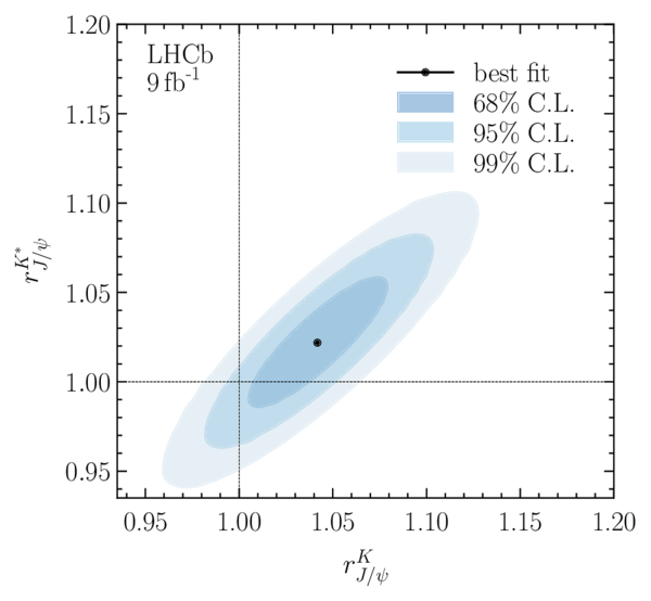
Two dimensional likelihood scans of (left) $ r_{ { J \mskip -3mu/\mskip -2mu\psi } }^{ K }$ vs. $ r_{ { J \mskip -3mu/\mskip -2mu\psi } }^{ K ^* }$ and (right) $ R_{\psi {(2S)} }^{ K }$ vs. $ R_{\psi {(2S)} }^{ K ^* }$ . The contours show the 68%, 95% and 99% C.L. regions and the solid markers show the best fit values.

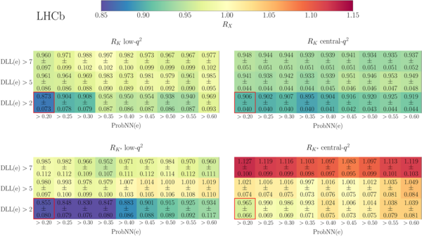
Results of the nominal fit without modeling of misidentified backgrounds as a function of the PID criteria used. The bins are, from top left to bottom right: $ R_K$ low- $ q^2$ , $ R_K$ $\text{central-} q^2 $ , $ R_{ K ^* }$ $\text{low-} q^2 $ and $ R_{ K ^* }$ $\text{central-} q^2 $ . The nominal set of criteria is highlighted in red. The quoted uncertainties are statistical only.

Shifts of the central value results from varying the PID criteria on electrons while modeling misidentified backgrounds in the fit. Particle selection criteria are varied to an intermediate working point reducing the expected contamination by a factor two, and to a tighter working point reducing the contamination by more than 75%. The bins are, from top left to right: $ R_K$ low- $ q^2$ , $ R_K$ $\text{central-} q^2 $ , $ R_{ K ^* }$ $\text{low-} q^2 $ and $ R_{ K ^* }$ $\text{central-} q^2 $ . The quoted relative uncertainties are statistical only.

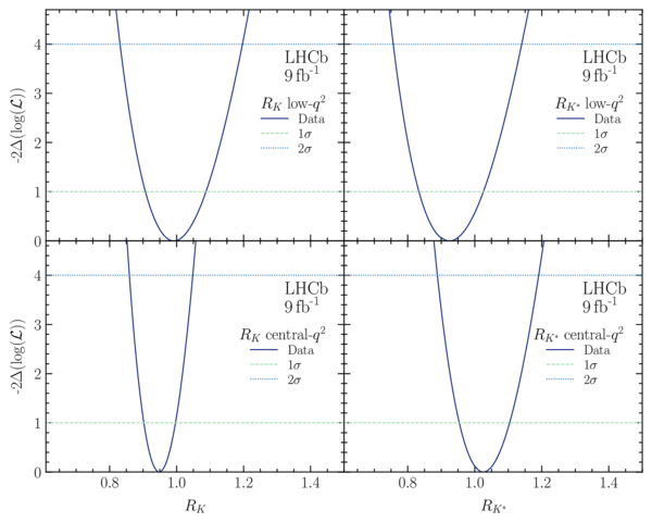
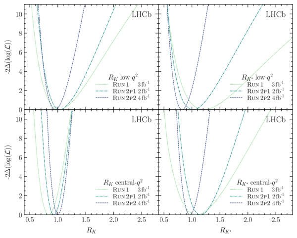
Likelihood scans for the LU observables (left) $ R_K$ and (right) $ R_{ K ^* }$ , in the (top) $\text{low-} q^2 $ and (bottom) $\text{central-} q^2 $ regions.

Correlation factors between the $ R_K$ and $ R_{ K ^* }$ results in the low- and $\text{central-} q^2 $ regions.

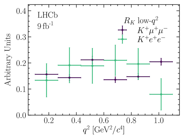
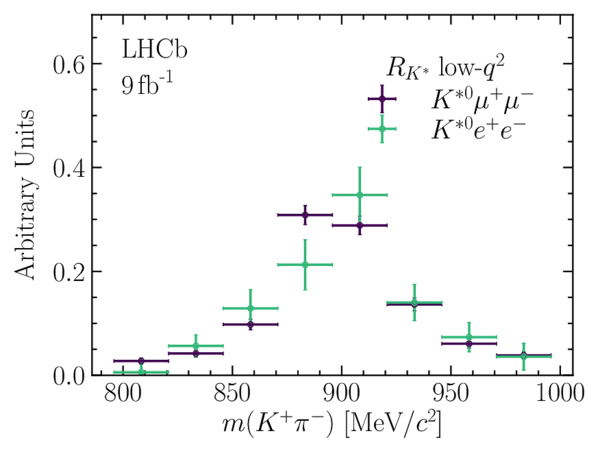
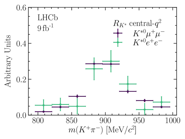
Background-subtracted distributions of quantities describing the $ B ^+ \rightarrow K ^+ \ell^+ \ell^- $ and $ B ^0 \rightarrow K ^{*0} \ell^+ \ell^- $ decays. The $\text{low-} q^2 $ region is plotted on the left, the $\text{central-} q^2 $ region on the right. The top and middle rows show the distributions of $ q^2$ for the $ B ^+ $ and $ B ^0$ signals, respectively. The bottom row shows the distribution of the $ K ^{*0}$ mass for the $ B ^0$ signals.

Measured values of LU observables in $ B ^+ \rightarrow K ^+ \ell^+ \ell^- $ and $ B ^0 \rightarrow K ^{*0} \ell^+ \ell^- $ decays and their overall compatibility with the SM.

One-dimensional likelihood scans for $ R_K$ and $ R_{ K ^* }$ in the low- and $\text{central-} q^2 $ regions, performing the measurements in each data-taking period separately. The scan shown includes both systematic and statistical uncertainties.

Animated gif made out of all figures.

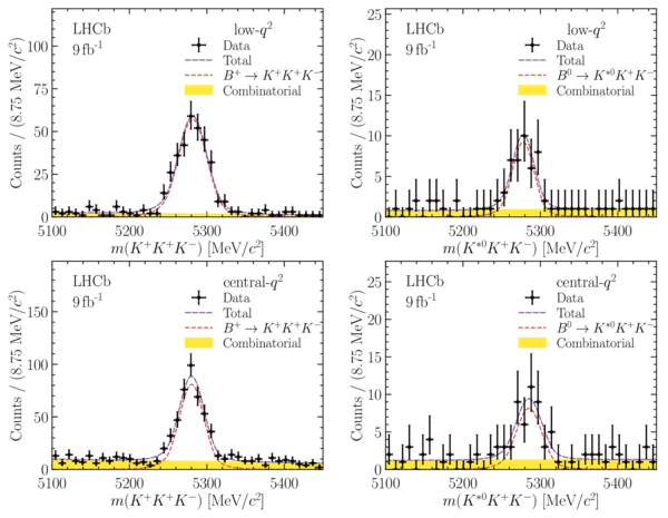
Exclusive backgrounds modeled in the $ B ^+ \rightarrow K ^+ \ell^+ \ell^- $ invariant mass fits, along with the $ q^2$ region of interest and the mode(s) for which the background is relevant.

Exclusive backgrounds modeled in the $ B ^0 \rightarrow K ^{*0} \ell^+ \ell^- $ invariant mass fits, the $ q^2$ region of interest and the mode(s) for which the background is relevant. The $K-\pi$ swap backgrounds refer to cases where the mass hypotheses of the kaon and pion from a genuine $ B ^0 \rightarrow K ^{*0} \ell^+ \ell^- $ decay are swapped.

Single-particle misidentification rates obtained on data averaging over the kinematics of prompt $D^{\ast+}\rightarrow D^{0}(\rightarrow K^{-}\pi^{+})\pi^{+}$ decays. The misidentification rates are evaluated for the PID criteria used in this analysis given the acceptance and kinematic requirements applied in the track final state. The misidentification rates corresponding to the PID requirements of Ref. [24] are given in parentheses.

Overall signal efficiency for electron mode in percent. The impact of global event cuts on the efficiency determination is not included as it cancels in the $ R_{(K, K ^* )}$ ratio defined in Eq. 2. The efficiency values obtained applying the same PID requirements of Ref. [24] are given in parentheses.

Invariant mass ranges used in the fits. The fit type indicates where the dilepton invariant mass is constrained to the known $ { J \mskip -3mu/\mskip -2mu\psi }$ ( $\psi {(2S)}$ ) mass.

Observed yields of the six signal and control modes and their statistical uncertainties.

Analytical functions used to describe the signal and resonant control modes. The fit type refers to whether the dilepton invariant mass is constrained to that of the $ { J \mskip -3mu/\mskip -2mu\psi }$ ( $\psi {(2S)}$ ) resonance or not. Category refers to the bremsstrahlung category in the case of electron modes. Hypatia refers to a two-sided version of a generalized Crystal Ball distribution introduced in Ref. [87].

Values of the $ r_{ { J \mskip -3mu/\mskip -2mu\psi } }^{ K }$ and $ r_{ { J \mskip -3mu/\mskip -2mu\psi } }^{ K ^* }$ single ratios, as well as $ R_{\psi {(2S)} }^{ K }$ and $ R_{\psi {(2S)} }^{ K ^* }$ double ratios, calculated in different data-taking periods, trigger categories, and using the $w( B ^+ )$ or $w( B ^0 )$ calibration chains. The three uncertainties are, from left to right: statistical from the invariant mass fits, statistical from the finite simulated sample sizes, and the bootstrapping uncertainty on the simulation calibrations.

Sources of systematic uncertainties on the $ R_K$ and $ R_{ K ^* }$ measurements in the low- and $\text{central-} q^2 $ regions. All values are given in percent and relative to the measured central value. These values are indicative and are computed as weighted averages of systematic variations determined in each data-taking period and trigger category. The different sources of uncertainties are determined using a best linear unbiased estimator accounting for correlations between different data taking periods and trigger categories. The bottom row with the total systematic is estimated by combining the error matrices for each source in quadrature and performing a best linear unbiased estimation.

Measured values of the $ R_K$ and $ R_{ K ^* }$ observables in the low- and $\text{central-} q^2 $ regions, with the associated statistical and systematic uncertainties presented separately.

SM predictions and uncertainties from the \texttt{flavio} software package [71]. The dominant QED uncertainty from Ref. [14] is quoted separately.

Measured values of the LU observables obtained from the separate run periods. Uncertainties are split into statistical and systematic components and have been extracted from the one-dimensional likelihood scans.