Study of charmonium decays to $K^0_S K \pi$ in the $B \to (K^0_S K \pi) K$ channels

Information

LHCb-PAPER-2022-051
CERN-EP-2023-060
arXiv:2304.14891 [PDF]

(Submitted on 28 Apr 2023)
PRD
Inspire 2655326

Tools

Abstract

A study of the $B^+\to K^0_SK^+K^-\pi^+$ and $B^+\to K^0_SK^+K^+\pi^-$ decays is performed using proton-proton collisions at center-of-mass energies of 7, 8 and 13 TeV at the LHCb experiment. The $K^0_SK \pi$ invariant mass spectra from both decay modes reveal a rich content of charmonium resonances. New precise measurements of the $\eta_c$ and $\eta_c(2S)$ resonance parameters are performed and branching fraction measurements are obtained for $B^+$ decays to $\eta_c$, $J/\psi$, $\eta_c(2S)$ and $\chi_{c1}$ resonances. In particular, the first observation and branching fraction measurement of $B^+ \to \chi_{c0} K^0 \pi^+$ is reported as well as first measurements of the $B^+\to K^0K^+K^-\pi^+$ and $B^+\to K^0K^+K^+\pi^-$ branching fractions. Dalitz plot analyses of $\eta_c \to K^0_SK\pi$ and $\eta_c(2S) \to K^0_SK\pi$ decays are performed. A new measurement of the amplitude and phase of the $K \pi$ $S$-wave as functions of the $K \pi$ mass is performed, together with measurements of the $K^*_0(1430)$, $K^*_0(1950)$ and $a_0(1700)$ parameters. Finally, the branching fractions of $\chi_{c1}$ decays to $K^*$ resonances are also measured.

Figures and captions

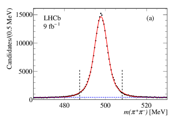
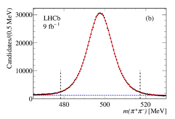
Invariant $\pi ^+ \pi ^- $ mass distribution for (a) $ K ^0_{\mathrm{SLL}}$ and (b) $ K ^0_{\mathrm{SDD}}$ candidates. The full (red) line indicates the fit results and the dashed (blue) line the background contribution. The vertical dashed lines indicate the region used to select the $ K ^0_{\mathrm{S}}$ signal.	fig1a.pdf [20 KiB] HiDef png [154 KiB] Thumbnail [121 KiB] *.C file
	fig1b.pdf [19 KiB] HiDef png [156 KiB] Thumbnail [122 KiB] *.C file
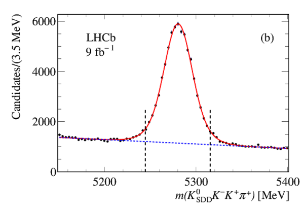
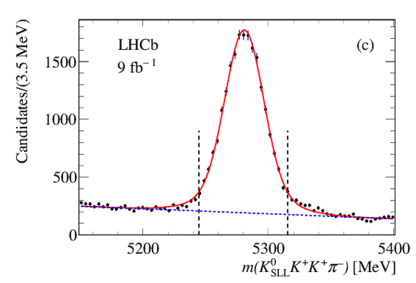
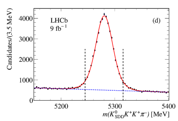
Distributions of $ K ^0_{\mathrm{S}} K ^+ K ^- \pi ^+ $ invariant mass for (a) $ K ^0_{\mathrm{SLL}}$ and (b) $ K ^0_{\mathrm{SDD}}$ candidates and distributions of $ K ^0_{\mathrm{S}} K ^+ K ^+ \pi ^- $ invariant mass for (c) $ K ^0_{\mathrm{SLL}}$ and (d) $ K ^0_{\mathrm{SDD}}$ candidates. The full (red) lines indicate the signal component and the dashed (blue) lines the background. The vertical dashed lines indicate the regions used to select the $ B ^+ $ signals.	fig2a.pdf [18 KiB] HiDef png [167 KiB] Thumbnail [133 KiB] *.C file
	fig2b.pdf [18 KiB] HiDef png [159 KiB] Thumbnail [123 KiB] *.C file
	fig2c.pdf [18 KiB] HiDef png [167 KiB] Thumbnail [130 KiB] *.C file
	fig2d.pdf [18 KiB] HiDef png [166 KiB] Thumbnail [134 KiB] *.C file
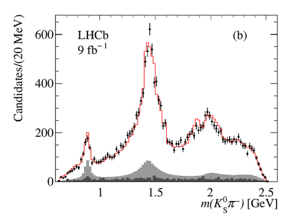
Invariant $ K ^0_{\mathrm{S}} K\pi$ mass distributions for (a) $ B^+\rightarrow K ^0_{\mathrm{S}} K ^+ K ^- \pi ^+ $ and (b) $ B^+\rightarrow K ^0_{\mathrm{S}} K ^+ K ^+ \pi ^- $ candidates (two entries per event).	fig3a.pdf [60 KiB] HiDef png [120 KiB] Thumbnail [65 KiB] *.C file
	fig3b.pdf [61 KiB] HiDef png [122 KiB] Thumbnail [66 KiB] *.C file
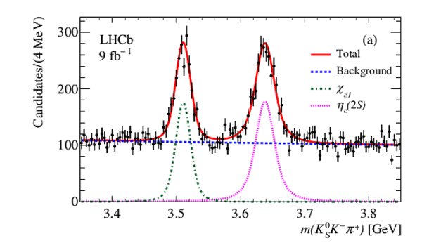
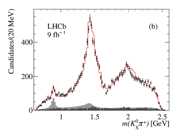
Invariant $ K ^0_{\mathrm{S}} K\pi$ invariant mass distributions, with the known $ { J \mskip -3mu/\mskip -2mu\psi }$ mass subtracted, in the $\eta _ c $ -- $ { J \mskip -3mu/\mskip -2mu\psi }$ mass region for (a) $ B^+\rightarrow K ^0_{\mathrm{S}} K ^+ K ^- \pi ^+ $ and (b) $ B^+\rightarrow K ^0_{\mathrm{S}} K ^+ K ^+ \pi ^- $ candidates. The results of the fits are overlayed.	fig4a.pdf [46 KiB] HiDef png [234 KiB] Thumbnail [150 KiB] *.C file
	fig4b.pdf [46 KiB] HiDef png [236 KiB] Thumbnail [154 KiB] *.C file
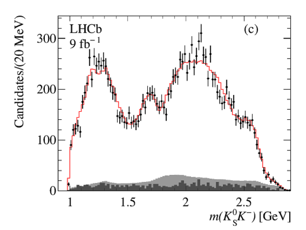
Invariant $ K ^0_{\mathrm{S}} K\pi$ mass distributions in the $\chi _{ c 1}$ -- $\eta_c(2S)$ mass region for (a) $ B^+\rightarrow K ^0_{\mathrm{S}} K ^+ K ^- \pi ^+ $ and (b) $ B^+\rightarrow K ^0_{\mathrm{S}} K ^+ K ^+ \pi ^- $ candidates. The results of the fits are overlayed.	fig5a.pdf [34 KiB] HiDef png [244 KiB] Thumbnail [176 KiB] *.C file
	fig5b.pdf [34 KiB] HiDef png [217 KiB] Thumbnail [158 KiB] *.C file
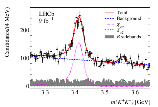
Invariant $ K ^+ K ^- $ mass distribution in the $\chi _{ c 0}$ - $\chi _{ c 2}$ mass region for $ B^+\rightarrow K ^0_{\mathrm{S}} K ^+ K ^- \pi ^+ $ decays. The two $ K ^0_{\mathrm{S}}$ datasets are combined. The results of the fit are overlayed. The curves also include interference terms and therefore the $\chi _{ c 0}$ lineshape takes slightly negative values.	fig6.pdf [31 KiB] HiDef png [262 KiB] Thumbnail [211 KiB] *.C file
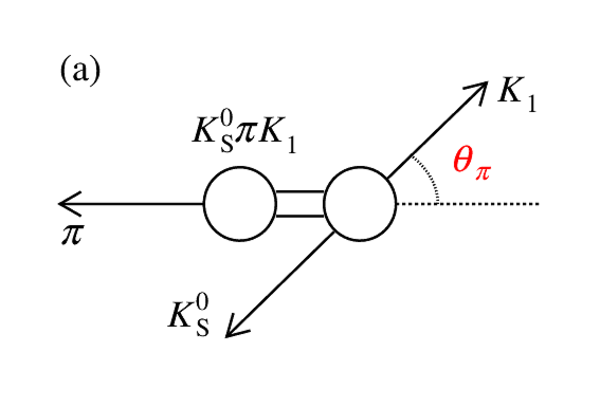
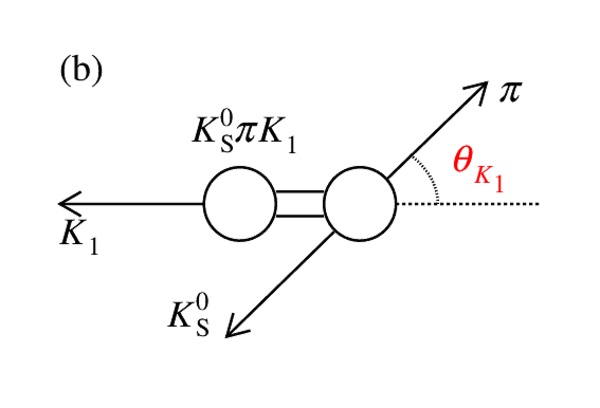
Definition of the angles (a) $\theta_{\pi}$, (b) $\theta_{K_1}$ and (c) $\phi_K$.	fig7a.pdf [13 KiB] HiDef png [77 KiB] Thumbnail [71 KiB] *.C file
	fig7b.pdf [13 KiB] HiDef png [79 KiB] Thumbnail [71 KiB] *.C file
	fig7c.pdf [12 KiB] HiDef png [79 KiB] Thumbnail [73 KiB] *.C file
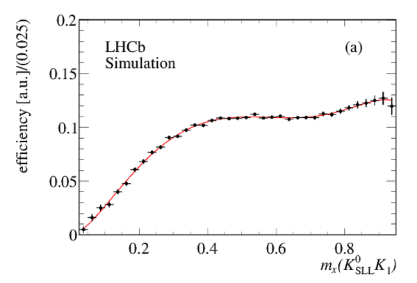
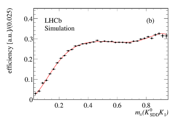
Efficiency projections (in arbitrary units) on $m_x( K ^0_{\mathrm{S}} K_1)$ for the (a) $ K ^0_{\mathrm{SLL}}$ and (b) $ K ^0_{\mathrm{SDD}}$ samples for the total $ B^+\rightarrow K ^0_{\mathrm{S}} K ^+ K ^- \pi ^+ $ dataset. The curves are the results of fits made using seventh-order polynomials.	fig8a.pdf [16 KiB] HiDef png [120 KiB] Thumbnail [104 KiB] *.C file
	fig8b.pdf [16 KiB] HiDef png [120 KiB] Thumbnail [105 KiB] *.C file
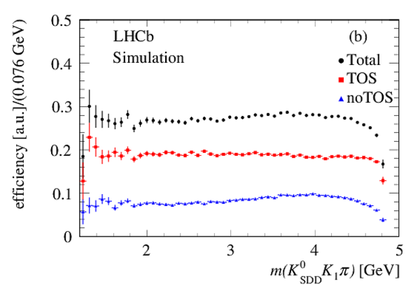
Efficiency projections (in arbitrary units) on $m( K ^0_{\mathrm{S}} K_1 \pi)$ for the (a) $ K ^0_{\mathrm{SLL}}$ and (b) $ K ^0_{\mathrm{SDD}}$ simulation samples separated for trigger conditions.	fig9a.pdf [21 KiB] HiDef png [176 KiB] Thumbnail [152 KiB] *.C file
	fig9b.pdf [20 KiB] HiDef png [170 KiB] Thumbnail [152 KiB] *.C file
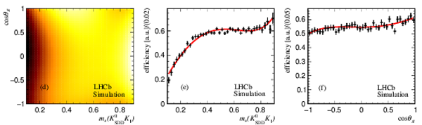
Two-dimensional efficiency fitted distributions in the $\eta _ c $ mass region for the (a) $ K ^0_{\mathrm{SLL}}$ and (d) $ K ^0_{\mathrm{SDD}}$ samples. Efficiency projections (in arbitrary units) for (b)-(c) $ K ^0_{\mathrm{SLL}}$ and (e)-(f) $ K ^0_{\mathrm{SDD}}$ simulation. The curves are the results from the fits according to Eq. 14.	fig10a.pdf [34 KiB] HiDef png [288 KiB] Thumbnail [174 KiB] *.C file
	fig10b.pdf [34 KiB] HiDef png [280 KiB] Thumbnail [166 KiB] *.C file
Efficiency projections (in arbitrary units) in the $\chi _{ c 1}$ -- $\eta_c(2S)$ mass region for the (a)-(b) $ K ^0_{\mathrm{SLL}}$ and (c)-(d) $ K ^0_{\mathrm{SDD}}$ simulation. The curves are the results from fits performed using seventh-order polynomials.	fig11a.pdf [21 KiB] HiDef png [165 KiB] Thumbnail [150 KiB] *.C file
	fig11b.pdf [21 KiB] HiDef png [164 KiB] Thumbnail [151 KiB] *.C file
Invariant $ K ^0_{\mathrm{S}} K\pi$ mass distributions in the $\eta _ c $ -- $ { J \mskip -3mu/\mskip -2mu\psi }$ signal region combining the $ K ^0_{\mathrm{SLL}}$ and $ K ^0_{\mathrm{SDD}}$ data for (a) $ B^+\rightarrow K ^0_{\mathrm{S}} K ^+ K ^- \pi ^+ $ and (b) $ B^+\rightarrow K ^0_{\mathrm{S}} K ^+ K ^+ \pi ^- $ decays. The dark-gray area represents the $ K ^0_{\mathrm{S}} K\pi$ invariant-mass spectrum from the $ B ^+ $ sideband; the light-gray areas indicate the $\eta _ c $ signal and sideband regions.	fig12a.pdf [30 KiB] HiDef png [135 KiB] Thumbnail [78 KiB] *.C file
	fig12b.pdf [30 KiB] HiDef png [136 KiB] Thumbnail [77 KiB] *.C file
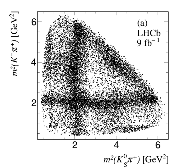
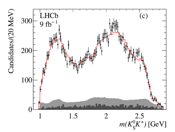
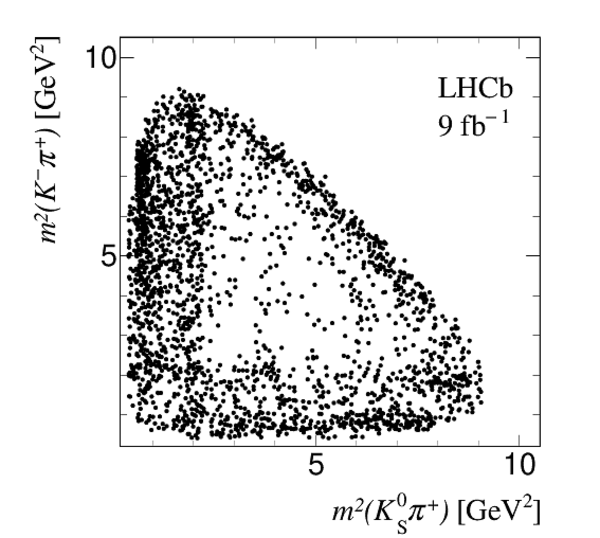
Dalitz plot of $\eta _ c \rightarrow K ^0_{\mathrm{S}} K\pi $ decays for (a) $ B^+\rightarrow K ^0_{\mathrm{S}} K ^+ K ^- \pi ^+ $ and (b) $ K ^0_{\mathrm{S}} K ^+ K ^+ \pi ^- $ . The empty horizontal band in (b) is due to the removal of the $\overline{ D } {}^0 \rightarrow K ^+ \pi ^- $ channel.	fig13a.pdf [473 KiB] HiDef png [634 KiB] Thumbnail [271 KiB] *.C file
	fig13b.pdf [495 KiB] HiDef png [641 KiB] Thumbnail [270 KiB] *.C file
Fit projections on the $ K ^- \pi ^+ $, $ K ^0_{\mathrm{S}} \pi ^+ $ and $ K ^0_{\mathrm{S}} K ^- $ invariant-mass distributions from the Dalitz-plot analysis of the $\eta _ c $ decay using the QMI model for $ B^+\rightarrow K ^0_{\mathrm{S}} K ^+ K ^- \pi ^+ $ data.	fig14a.pdf [28 KiB] HiDef png [181 KiB] Thumbnail [159 KiB] *.C file
	fig14b.pdf [28 KiB] HiDef png [161 KiB] Thumbnail [140 KiB] *.C file
	fig14c.pdf [28 KiB] HiDef png [174 KiB] Thumbnail [158 KiB] *.C file
Fit projections on the $ K ^+ \pi ^- $, $ K ^0_{\mathrm{S}} \pi ^- $ and $ K ^0_{\mathrm{S}} K ^+ $ invariant-mass distributions from the Dalitz-plot analysis of $\eta _ c $ decay using the QMI model for the $ B^+\rightarrow K ^0_{\mathrm{S}} K ^+ K ^+ \pi ^- $ data.	fig15a.pdf [28 KiB] HiDef png [183 KiB] Thumbnail [162 KiB] *.C file
	fig15b.pdf [28 KiB] HiDef png [165 KiB] Thumbnail [147 KiB] *.C file
	fig15c.pdf [28 KiB] HiDef png [173 KiB] Thumbnail [162 KiB] *.C file
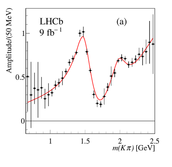
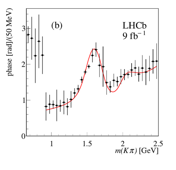
Comparisons between the fitted $K \pi$ {\it S}-wave (a) amplitude and (b) phase obtained from the (black) $ B^+\rightarrow K ^0_{\mathrm{S}} K ^+ K ^- \pi ^+ $ and (red) $ B^+\rightarrow K ^0_{\mathrm{S}} K ^+ K ^+ \pi ^- $ data. Note that the point at 1.425 $\text{ Ge V}$ is fixed at values 1.0 and 1.57 for amplitude and phase, respectively, and therefore there is no associated uncertainty. The plotted uncertainties are obtained averaging the uncertainties on the two adjacent mass measurements.	fig16.pdf [24 KiB] HiDef png [197 KiB] Thumbnail [156 KiB] *.C file
Argand diagram for the $K \pi$ {\it S}-wave averaged over the QMI results from $ B^+\rightarrow K ^0_{\mathrm{S}} K ^+ K ^- \pi ^+ $ and $ B^+\rightarrow K ^0_{\mathrm{S}} K ^+ K ^+ \pi ^- $ data.	fig17.pdf [17 KiB] HiDef png [182 KiB] Thumbnail [145 KiB] *.C file
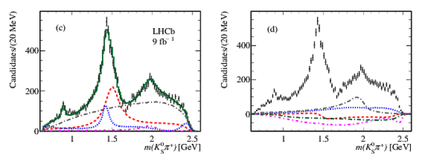
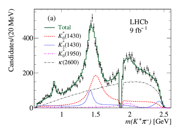
Fit projections on the $ K ^- \pi ^+ $, $ K ^0_{\mathrm{S}} \pi ^+ $ and $ K ^0_{\mathrm{S}} K ^- $ invariant-mass distributions from the Dalitz-plot analysis of the $\eta _ c $ decay using the isobar model for the $ B^+\rightarrow K ^0_{\mathrm{S}} K ^+ K ^- \pi ^+ $ data. Panels (a, c, e) show the most important resonant contributions. To simplify the plots, only resonant contributions relative to that mass projection are shown. Panels (b, d, f) show the interference terms for contributions greater than 3%. The legend in (a) also applies to (c) and the legend in (b) also applies to (d) and (f).	fig18a.pdf [39 KiB] HiDef png [237 KiB] Thumbnail [174 KiB] *.C file
	fig18b.pdf [39 KiB] HiDef png [196 KiB] Thumbnail [141 KiB] *.C file
	fig18c.pdf [36 KiB] HiDef png [215 KiB] Thumbnail [159 KiB] *.C file
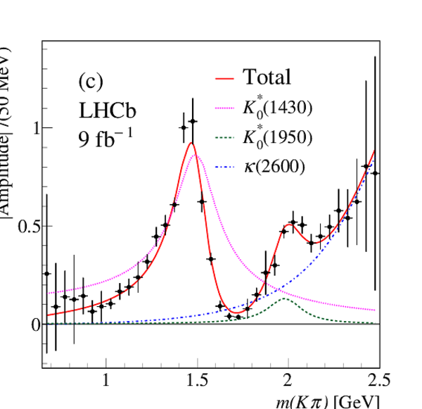
Fit to the (a) amplitude, (b) phase and (c) squared amplitude from the $\eta _ c $ QMI analysis using the results from the isobar-model analysis. The black points are obtained using the inverse-variance-weighted averages of the $ B^+\rightarrow K ^0_{\mathrm{S}} K ^+ K ^- \pi ^+ $ and $ B^+\rightarrow K ^0_{\mathrm{S}} K ^+ K ^+ \pi ^- $ data. The error bars are computed as the quadratic sum of the statistical and systematic uncertainties. The phase measurements in the $K \pi$ mass region below 0.90 $\text{ Ge V}$ are not included in the fit.	fig19a.pdf [16 KiB] HiDef png [153 KiB] Thumbnail [120 KiB] *.C file
	fig19b.pdf [16 KiB] HiDef png [144 KiB] Thumbnail [113 KiB] *.C file
	fig19c.pdf [19 KiB] HiDef png [242 KiB] Thumbnail [182 KiB] *.C file
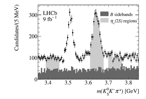
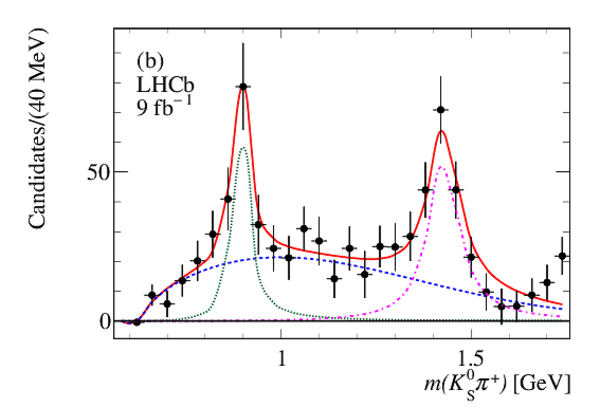
Invariant $ K ^0_{\mathrm{S}} K\pi$ mass distribution in the region of the $\eta_c(2S)$ resonance for $ B^+\rightarrow K ^0_{\mathrm{S}} K ^+ K ^- \pi ^+ $ . The $\eta_c(2S)$ signal and sideband regions are indicated in light gray, while the incoherent background estimated from the $ B ^+ $ sidebands is shown in dark gray.	fig20.pdf [27 KiB] HiDef png [126 KiB] Thumbnail [74 KiB] *.C file
Dalitz plot of $\eta_c(2S) \rightarrow K ^0_{\mathrm{S}} K\pi $ decays for the $ B^+\rightarrow K ^0_{\mathrm{S}} K ^+ K ^- \pi ^+ $ sample.	fig21.pdf [96 KiB] HiDef png [334 KiB] Thumbnail [179 KiB] *.C file
Dalitz-plot projections of the $\eta_c(2S) \rightarrow K ^0_{\mathrm{S}} K\pi $ decays from the $ B^+\rightarrow K ^0_{\mathrm{S}} K ^+ K ^- \pi ^+ $ sample. The solid red line shows the fit result, the light gray shaded area is the contribution from the fitted sidebands and the dark shaded gray area is the contribution from the $ B ^+ $ sidebands. The empty region in the $ K ^0_{\mathrm{S}} K ^- $ invariant-mass projection is due to the removal of the contribution from $ D ^+_ s \rightarrow K ^0_{\mathrm{S}} K ^- $ decays.	fig22a.pdf [25 KiB] HiDef png [157 KiB] Thumbnail [156 KiB] *.C file
	fig22b.pdf [25 KiB] HiDef png [175 KiB] Thumbnail [170 KiB] *.C file
	fig22c.pdf [25 KiB] HiDef png [157 KiB] Thumbnail [154 KiB] *.C file
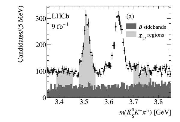
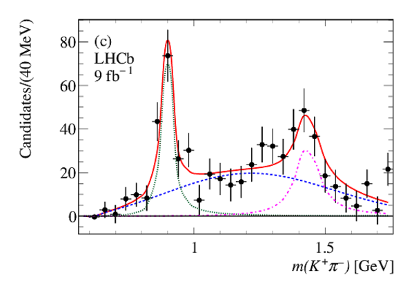
Invariant $ K ^0_{\mathrm{S}} K\pi$ mass distribution in the region of the $\chi _{ c 1}$ / $\eta_c(2S)$ resonances for (a) $ B^+\rightarrow K ^0_{\mathrm{S}} K ^+ K ^- \pi ^+ $ and (b) $ B^+\rightarrow K ^0_{\mathrm{S}} K ^+ K ^+ \pi ^- $ decays. In light gray are indicated the $\chi _{ c 1}$ signal region and sidebands. In dark gray is indicated the incoherent background estimated from the $ B ^+ $ sidebands.	fig23a.pdf [27 KiB] HiDef png [125 KiB] Thumbnail [74 KiB] *.C file
	fig23b.pdf [27 KiB] HiDef png [130 KiB] Thumbnail [77 KiB] *.C file
Dalitz plot of $\chi _{ c 1} \rightarrow K ^0_{\mathrm{S}} K ^- \pi ^+ $ decays for the $ B^+\rightarrow K ^0_{\mathrm{S}} K ^+ K ^- \pi ^+ $ sample.	fig24.pdf [85 KiB] HiDef png [284 KiB] Thumbnail [152 KiB] *.C file
Background-subtracted $K \pi$ and $ K ^0_{\mathrm{S}} \pi$ invariant-mass spectra from $\chi _{ c 1} \rightarrow K ^0_{\mathrm{S}} K\pi $ decays for the (a)-(b) $ B^+\rightarrow K ^0_{\mathrm{S}} K ^+ K ^- \pi ^+ $ and (c)-(d) $ B^+\rightarrow K ^0_{\mathrm{S}} K ^+ K ^+ \pi ^- $ data. The results of the fits are overlaid.	fig25a.pdf [18 KiB] HiDef png [223 KiB] Thumbnail [175 KiB] *.C file
	fig25b.pdf [18 KiB] HiDef png [195 KiB] Thumbnail [143 KiB] *.C file
	fig25c.pdf [18 KiB] HiDef png [202 KiB] Thumbnail [149 KiB] *.C file
	fig25d.pdf [18 KiB] HiDef png [198 KiB] Thumbnail [149 KiB] *.C file
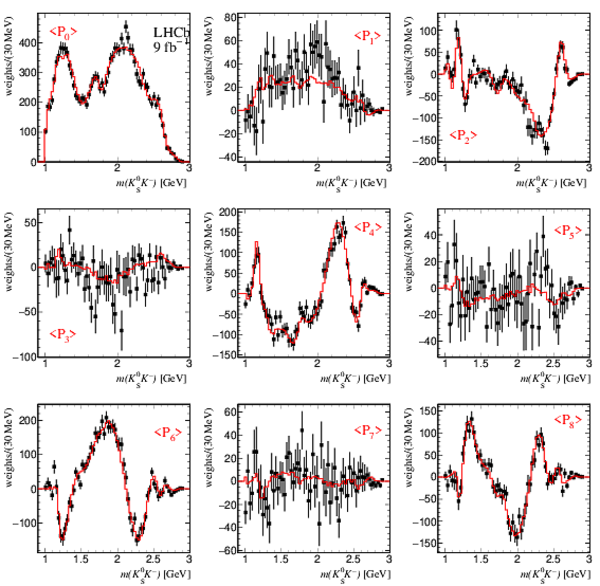
Projected $ K ^- \pi ^+ $ invariant mass spectra weighted by Legendre polynomial moments $P_L(\cos\theta_{ K ^0_{\mathrm{S}} })$ for $\eta _ c \rightarrow K ^0_{\mathrm{S}} K ^- \pi ^+ $ from $ B^+\rightarrow K ^0_{\mathrm{S}} K ^+ K ^- \pi ^+ $ data. The drawn curves result from the Dalitz plot fit using the QMI method described in the text.	fig26.pdf [59 KiB] HiDef png [595 KiB] Thumbnail [402 KiB] *.C file
Projected $ K ^0_{\mathrm{S}} \pi ^+ $ invariant mass spectra weighted by Legendre polynomial moments $P_L(\cos\theta_{ K ^- })$ for $\eta _ c \rightarrow K ^0_{\mathrm{S}} K ^- \pi ^+ $ from $ B^+\rightarrow K ^0_{\mathrm{S}} K ^+ K ^- \pi ^+ $ data. The drawn curves result from the Dalitz plot fit using the QMI method described in the text.	fig27.pdf [58 KiB] HiDef png [606 KiB] Thumbnail [400 KiB] *.C file
Projected $ K ^0_{\mathrm{S}} K ^- $ invariant mass spectra weighted by Legendre polynomial moments $P_L(\cos\theta_{\pi ^+ })$ for $\eta _ c \rightarrow K ^0_{\mathrm{S}} K ^- \pi ^+ $ from $ B^+\rightarrow K ^0_{\mathrm{S}} K ^+ K ^- \pi ^+ $ data. The drawn curves result from the Dalitz plot fit using the QMI method described in the text.	fig28.pdf [46 KiB] HiDef png [620 KiB] Thumbnail [433 KiB] *.C file
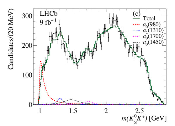
Fit projections on the (a) $ K ^+ \pi ^- $, (b) $ K ^0_{\mathrm{S}} \pi ^- $ and (c) $ K ^0_{\mathrm{S}} K ^+ $ invariant mass distributions from the Dalitz-plot analysis of the $\eta _ c $ decay using the isobar model for $ B^+\rightarrow K ^0_{\mathrm{S}} K ^+ K ^+ \pi ^- $ data. The curves show the most important resonant contributions. To simplify the plots only resonant contributions relative to that mass projection are shown. The legend in (a) applies also to (b).	fig29a.pdf [26 KiB] HiDef png [262 KiB] Thumbnail [201 KiB] *.C file
	fig29b.pdf [25 KiB] HiDef png [217 KiB] Thumbnail [163 KiB] *.C file
	fig29c.pdf [24 KiB] HiDef png [245 KiB] Thumbnail [195 KiB] *.C file
Animated gif made out of all figures.	PAPER-2022-051.gif Thumbnail

Tables and captions

Fitted $ B ^+ $ signal yield and purity for $ B^+\rightarrow K ^0_{\mathrm{S}} K ^+ K ^- \pi ^+ $ and $ B^+\rightarrow K ^0_{\mathrm{S}} K ^+ K ^+ \pi ^- $ final states separated by $ K ^0_{\mathrm{S}}$ type.	Table_1.pdf [61 KiB] HiDef png [70 KiB] Thumbnail [34 KiB] tex code
Fitted $\eta _ c $ , $ { J \mskip -3mu/\mskip -2mu\psi }$ , $\eta_c(2S)$ and $\chi _{ c 1}$ parameters. For the $ { J \mskip -3mu/\mskip -2mu\psi }$ the $m'=m-m_{ { J \mskip -3mu/\mskip -2mu\psi } }$ value is reported. The first uncertainty is statistical, the second systematic.	Table_2.pdf [71 KiB] HiDef png [92 KiB] Thumbnail [38 KiB] tex code
Summary of systematic uncertainties on $ { J \mskip -3mu/\mskip -2mu\psi }$ and $\eta _ c $ resonance parameters.	Table_3.pdf [72 KiB] HiDef png [105 KiB] Thumbnail [46 KiB] tex code
List of the systematic uncertainties on the $\chi _{ c 1}$ and $\eta_c(2S)$ parameters.	Table_4.pdf [71 KiB] HiDef png [92 KiB] Thumbnail [42 KiB] tex code
Candidate events and purities in the $\eta _ c $ signal region and fractions of $ B ^+ $ sideband contributions in the $\eta _ c $ sideband regions for $ B^+\rightarrow K ^0_{\mathrm{S}} K ^+ K ^- \pi ^+ $ and $ B^+\rightarrow K ^0_{\mathrm{S}} K ^+ K ^+ \pi ^- $ decays. Low and high indicate the lower and higher sideband candidates. Because of the limited statistics, the values of $f_B$ are summed for the $ K ^0_{\mathrm{SLL}}$ and $ K ^0_{\mathrm{SDD}}$ data.	Table_5.pdf [69 KiB] HiDef png [41 KiB] Thumbnail [18 KiB] tex code
Results from the Dalitz-plot analysis of the $\eta _ c $ decay in (top) $ B^+\rightarrow K ^0_{\mathrm{S}} K ^+ K ^- \pi ^+ $ , (center) $ B^+\rightarrow K ^0_{\mathrm{S}} K ^+ K ^+ \pi ^- $ and (bottom) inverse-variance-weighted averages. The QMI model is used for the $K \pi$ {\it S}-wave.	Table_6.pdf [71 KiB] HiDef png [210 KiB] Thumbnail [106 KiB] tex code
Fractional interference contributions from the Dalitz-plot analysis of the $\eta _ c $ decay in $ B^+\rightarrow K ^0_{\mathrm{S}} K ^+ K ^- \pi ^+ $ decays using the QMI model. Absolute values less than 3% are not listed.	Table_7.pdf [67 KiB] HiDef png [76 KiB] Thumbnail [33 KiB] tex code
Systematic uncertainties on (left) fractional contributions (%) and (right) phases (rad) in the $\eta _ c $ Dalitz-plot analysis in the $ B^+\rightarrow K ^0_{\mathrm{S}} K ^+ K ^- \pi ^+ $ decay using the QMI model for the $K \pi$ {\it S}-wave.	Table_8.pdf [61 KiB] HiDef png [83 KiB] Thumbnail [37 KiB] tex code
Systematic uncertainties on (left) fractional contributions (%) and (right) phases (rad) in the $\eta _ c $ Dalitz-plot analysis in the $ B^+\rightarrow K ^0_{\mathrm{S}} K ^+ K ^+ \pi ^- $ decay using the QMI model for the $K \pi$ {\it S}-wave.	Table_9.pdf [61 KiB] HiDef png [84 KiB] Thumbnail [37 KiB] tex code
Fitted parameters and significances of the resonances observed in the $\eta _ c $ Dalitz-plot analysis. Significances larger than 10$\sigma$ are evaluated as $\sqrt{\Delta(2 \log \cal L )}$.	Table_10.pdf [62 KiB] HiDef png [50 KiB] Thumbnail [24 KiB] tex code
Results from the Dalitz-plot analysis of the $\eta _ c $ using the isobar model for (top) $ B^+\rightarrow K ^0_{\mathrm{S}} K ^+ K ^- \pi ^+ $ decays, $ B^+\rightarrow K ^0_{\mathrm{S}} K ^+ K ^+ \pi ^- $ decays (center) and their inverse-variance-weighted averages (bottom).	Table_11.pdf [63 KiB] HiDef png [236 KiB] Thumbnail [106 KiB] tex code
Fractional interference contributions from the Dalitz-plot analysis of the $\eta _ c $ decay in $ B^+\rightarrow K ^0_{\mathrm{S}} K ^+ K ^- \pi ^+ $ decays using the isobar model. Absolute values less than 3% are not listed.	Table_12.pdf [60 KiB] HiDef png [160 KiB] Thumbnail [69 KiB] tex code
Candidate events in the signal region, purities, and $ B ^+ $ background contributions to the $\eta_c(2S) \rightarrow K ^0_{\mathrm{S}} K\pi $ Dalitz-plot analysis separated for $ K ^0_{\mathrm{S}}$ types. The incoherent background fractions $f_B$ in the low and high sidebands refer to the sum of the $ K ^0_{\mathrm{SLL}}$ and $ K ^0_{\mathrm{SDD}}$ data.	Table_13.pdf [60 KiB] HiDef png [30 KiB] Thumbnail [14 KiB] tex code
Systematic uncertainties on (left) fractional contributions (%) and (right) phases in the $\eta_c(2S)$ Dalitz-plot analysis in $ B^+\rightarrow K ^0_{\mathrm{S}} K ^+ K ^- \pi ^+ $ decay using the isobar model.	Table_14.pdf [54 KiB] HiDef png [72 KiB] Thumbnail [32 KiB] tex code
Results from the Dalitz-plot analysis of $\eta_c(2S) \rightarrow K ^0_{\mathrm{S}} K\pi $ in the $ B^+\rightarrow K ^0_{\mathrm{S}} K ^+ K ^- \pi ^+ $ final state using the isobar model.	Table_15.pdf [62 KiB] HiDef png [74 KiB] Thumbnail [37 KiB] tex code
Fractional interference contributions from the Dalitz plot analysis of the $\eta_c(2S)$ decay in $ B^+\rightarrow K ^0_{\mathrm{S}} K ^+ K ^- \pi ^+ $ decays using the isobar model. Absolute values less than 5% are not listed.	Table_16.pdf [60 KiB] HiDef png [112 KiB] Thumbnail [50 KiB] tex code
Candidate events and purities of $\chi _{ c 1}$ for the $ B^+\rightarrow K ^0_{\mathrm{S}} K ^+ K ^- \pi ^+ $ and $ B^+\rightarrow K ^0_{\mathrm{S}} K ^+ K ^+ \pi ^- $ final states separated for the $ K ^0_{\mathrm{SLL}}$ and $ K ^0_{\mathrm{SDD}}$ data. The incoherent background fractions $f_B$ values for the lower and higher sideband regions are computed for the sum of the $ K ^0_{\mathrm{SLL}}$ and $ K ^0_{\mathrm{SDD}}$ data.	Table_17.pdf [68 KiB] HiDef png [42 KiB] Thumbnail [18 KiB] tex code
Results from the fits to the $K \pi$ and $ K ^0_{\mathrm{S}} \pi$ background-subtracted invariant-mass distributions in the $\chi _{ c 1}$ decay for the (top) $ B^+\rightarrow K ^0_{\mathrm{S}} K ^+ K ^- \pi ^+ $ and (bottom) $ K ^0_{\mathrm{S}} K ^+ K ^+ \pi ^- $ data.	Table_18.pdf [69 KiB] HiDef png [78 KiB] Thumbnail [35 KiB] tex code
Inverse-variance-weighted averages of the fractional contributions for $\chi _{ c 1}$ decays to $K^\overline{ K } $ resonances from the $ B^+\rightarrow K ^0_{\mathrm{S}} K ^+ K ^- \pi ^+ $ and $ B^+\rightarrow K ^0_{\mathrm{S}} K ^+ K ^+ \pi ^- $ final states. The branching fractions of the $\chi _{ c 1} \rightarrow K ^0_{\mathrm{S}} K\pi $ decays to $K^{}(892)$ and the $K^{*}_2(1430)$ resonances are also included. The reported uncertainties are statistical, systematic and from the uncertainty on the $\chi _{ c 1}$ branching fraction (see text) [3].	Table_19.pdf [62 KiB] HiDef png [54 KiB] Thumbnail [26 KiB] tex code
Resulting yields and total charm fraction from the fits to the four-body, three-body and two-body invariant-mass spectra uncorrected for efficiency for the (top) $ B^+\rightarrow K ^0_{\mathrm{S}} K ^+ K ^- \pi ^+ $ and (bottom) $ B^+\rightarrow K ^0_{\mathrm{S}} K ^+ K ^+ \pi ^- $ data, separated by $ K ^0_{\mathrm{S}}$ category. The quoted uncertainties are statistical only.	Table_20.pdf [68 KiB] HiDef png [197 KiB] Thumbnail [94 KiB] tex code
Ratios of efficiency-corrected intermediate-resonance yields relative to the yield of the (top) $\eta _ c $ and (bottom) $ { J \mskip -3mu/\mskip -2mu\psi }$ resonances. The first uncertainty is statistical, the second systematic.	Table_21.pdf [62 KiB] HiDef png [142 KiB] Thumbnail [73 KiB] tex code
Measured branching fractions with the $\eta _ c $ resonance as a reference using the (top) $ B^+\rightarrow K ^0 K ^+ K ^- \pi ^+ $ and (bottom) $ B^+\rightarrow K ^0 K ^+ K ^+ \pi ^- $ data. The first uncertainty is statistical, the second systematic and the third due to the PDG uncertainty on the $ B ^+ \rightarrow \eta _ c K ^+ $ branching fraction.	Table_22.pdf [70 KiB] HiDef png [90 KiB] Thumbnail [45 KiB] tex code
Measured branching fractions with the $ { J \mskip -3mu/\mskip -2mu\psi }$ resonance as a reference using the (top) $ B^+\rightarrow K ^0 K ^+ K ^- \pi ^+ $ and (bottom) $ B^+\rightarrow K ^0 K ^+ K ^+ \pi ^- $ data. The first uncertainty is statistical, the second systematic, the third due to the PDG uncertainty on the $ B ^+ \rightarrow { J \mskip -3mu/\mskip -2mu\psi } K ^+ $ branching fraction.	Table_23.pdf [69 KiB] HiDef png [84 KiB] Thumbnail [43 KiB] tex code
Measured branching fractions using (top) the $\eta _ c $ and (bottom) the $ { J \mskip -3mu/\mskip -2mu\psi }$ resonance as reference for $ B^+\rightarrow K ^0 K ^+ K ^- \pi ^+ $ data. The first uncertainty is statistical, the second systematic, the third due to the PDG uncertainty on the $ B ^+ \rightarrow \eta _ c K ^+ $ or $ B ^+ \rightarrow { J \mskip -3mu/\mskip -2mu\psi } K ^+ $ branching fraction. The PDG reports an upper limit $ B ^+ \rightarrow \chi _{ c 0} K^{*+}<0.21 \times 10^{-3}$.	Table_24.pdf [68 KiB] HiDef png [57 KiB] Thumbnail [29 KiB] tex code
Inverse-variance averaged numerical values of the measured $K \pi$ {\it S}-wave as a function of the $K \pi$ mass. The first uncertainty is statistical, the second systematic. The values at $K \pi$ mass of 1.425 $\text{ Ge V}$ (in italics) are fixed.	Table_25.pdf [54 KiB] HiDef png [420 KiB] Thumbnail [206 KiB] tex code