

Compact Muon Solenoid
LHC, CERN
| CMS-B2G-14-002 ; CERN-PH-EP-2015-034 | ||
| Search for vector-like T quarks decaying to top quarks and Higgs bosons in the all-hadronic channel using jet substructure | ||
| CMS Collaboration | ||
| 6 March 2015 | ||
| J. High Energy Phys. 06 (2015) 080 | ||
| Abstract: A search is performed for a vector-like heavy T quark that is produced in pairs and that decays to a top quark and a Higgs boson. The data analysed correspond to an integrated luminosity of 19.7 fb$ ^{-1} $ collected with the CMS detector in proton-proton collisions at $ \sqrt{s} $ = 8 TeV. For T quarks with large mass values the top quarks and Higgs bosons can have significant Lorentz boosts, so that their individual decay products often overlap and merge. Methods are applied to resolve the substructure of such merged jets. Upper limits on the production cross section of a T quark with mass between 500 and 1000 GeV/$ c^2 $ are derived. If the T quark decays exclusively to tH, the observed (expected) lower limit on the mass of the T quark is 745 (773) GeV/$ c^2 $ at 95% confidence level. For the first time an algorithm is used for tagging boosted Higgs bosons that is based on a combination of jet substructure information and b tagging. | ||
| Links: e-print arXiv:1503.01952 [hep-ex] (PDF) ; CDS record ; inSPIRE record ; Public twiki page ; CADI line (restricted) ; | ||
| Figures | |

png pdf |
Figure 1-a:
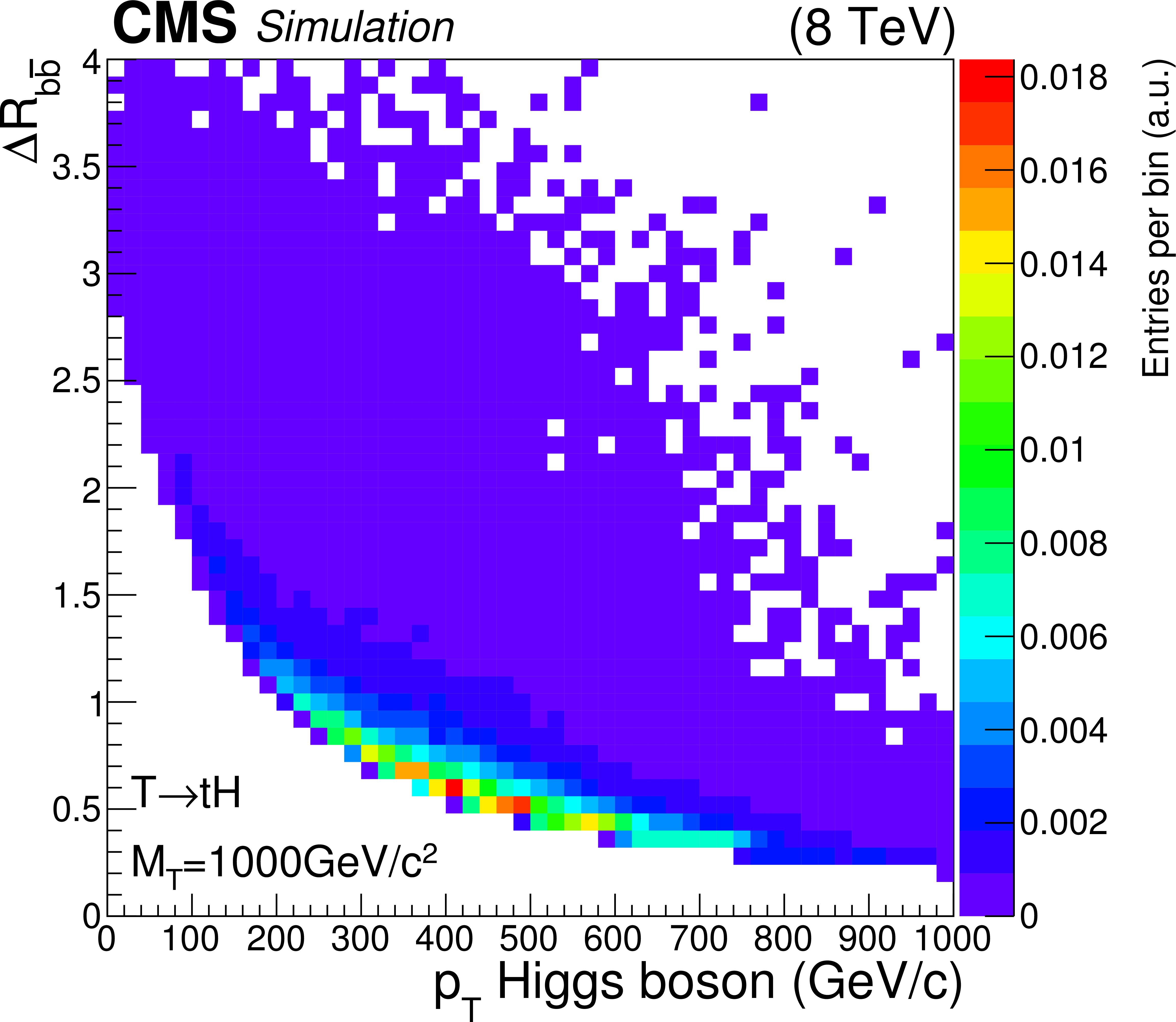
The distribution of the angular distance $\Delta R_{ {\mathrm {b}}ij}$ between the three top quark decay products as a function of the top quark $ {p_{\mathrm {T}}} $ for simulated T quark events with a T quark mass of 1000 GeV/$c^2$ (a). Distribution of the angular distance $\Delta R_{ { {\mathrm {b}} {\overline {\mathrm {b}}}} }$ of the two generated b quarks from Higgs boson decays versus the Higgs boson $ {p_{\mathrm {T}}} $, for the same event sample (b). |
png pdf |
Figure 1-b:
The distribution of the angular distance $\Delta R_{ {\mathrm {b}}ij}$ between the three top quark decay products as a function of the top quark $ {p_{\mathrm {T}}} $ for simulated T quark events with a T quark mass of 1000 GeV/$c^2$ (a). Distribution of the angular distance $\Delta R_{ { {\mathrm {b}} {\overline {\mathrm {b}}}} }$ of the two generated b quarks from Higgs boson decays versus the Higgs boson $ {p_{\mathrm {T}}} $, for the same event sample (b). |

png pdf |
Figure 2-a:
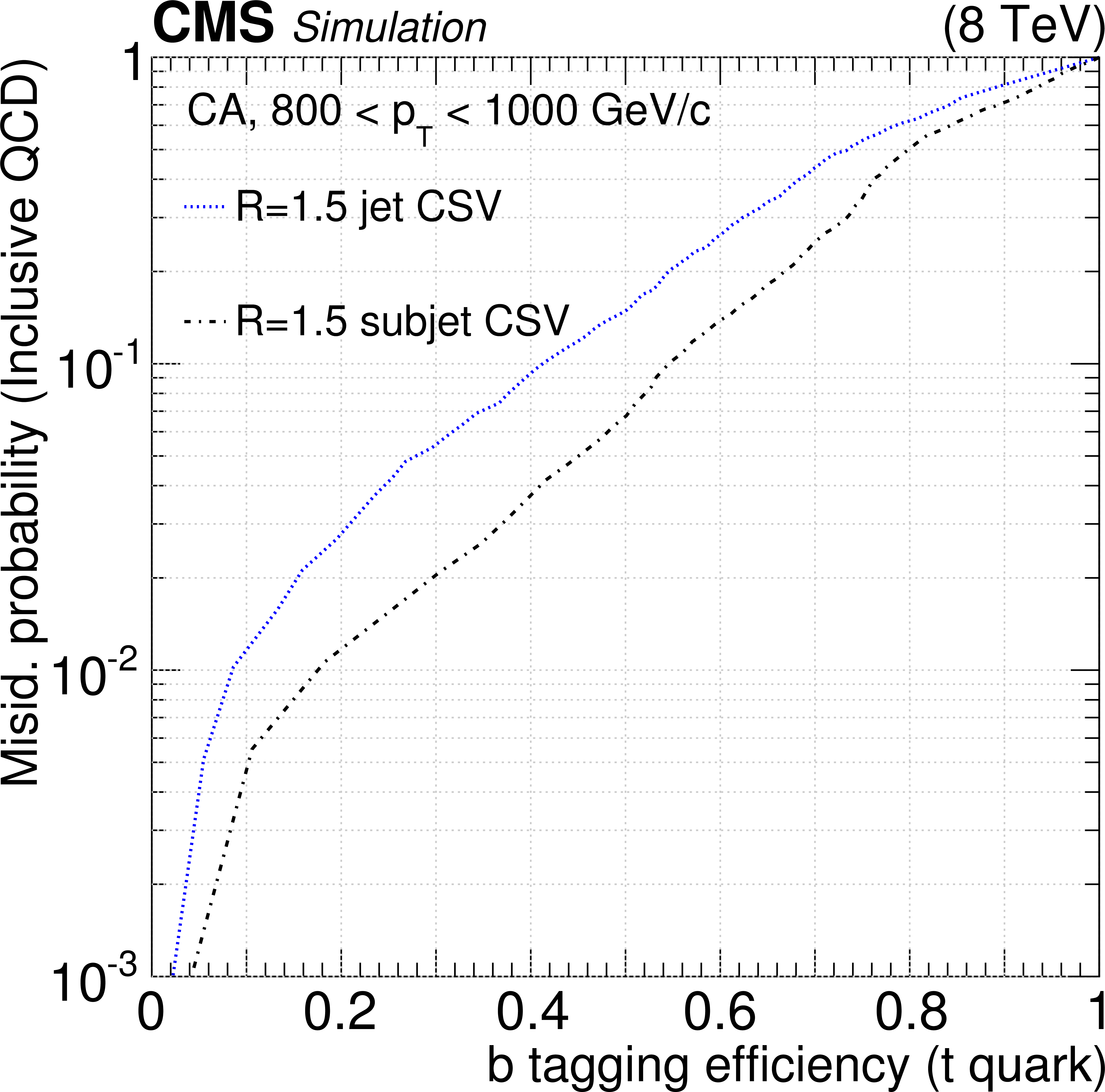
Performance of the CSV b tagging algorithm in simulated events with CA15 jets and with subjets within the same CA15 jet. The misidentification probability for inclusive QCD jets is shown versus the b tagging efficiency for boosted top quarks originating from T quark decays, for CA15 jet transverse momentum ranges of (a) 200 $< {p_{\mathrm {T}}} <$ 400 GeV/$c$ and (b) 800 $< {p_{\mathrm {T}}} <$ 1000 GeV/$c$. |
png pdf |
Figure 2-b:
Performance of the CSV b tagging algorithm in simulated events with CA15 jets and with subjets within the same CA15 jet. The misidentification probability for inclusive QCD jets is shown versus the b tagging efficiency for boosted top quarks originating from T quark decays, for CA15 jet transverse momentum ranges of (a) 200 $< {p_{\mathrm {T}}} <$ 400 GeV/$c$ and (b) 800 $< {p_{\mathrm {T}}} <$ 1000 GeV/$c$. |
png pdf |
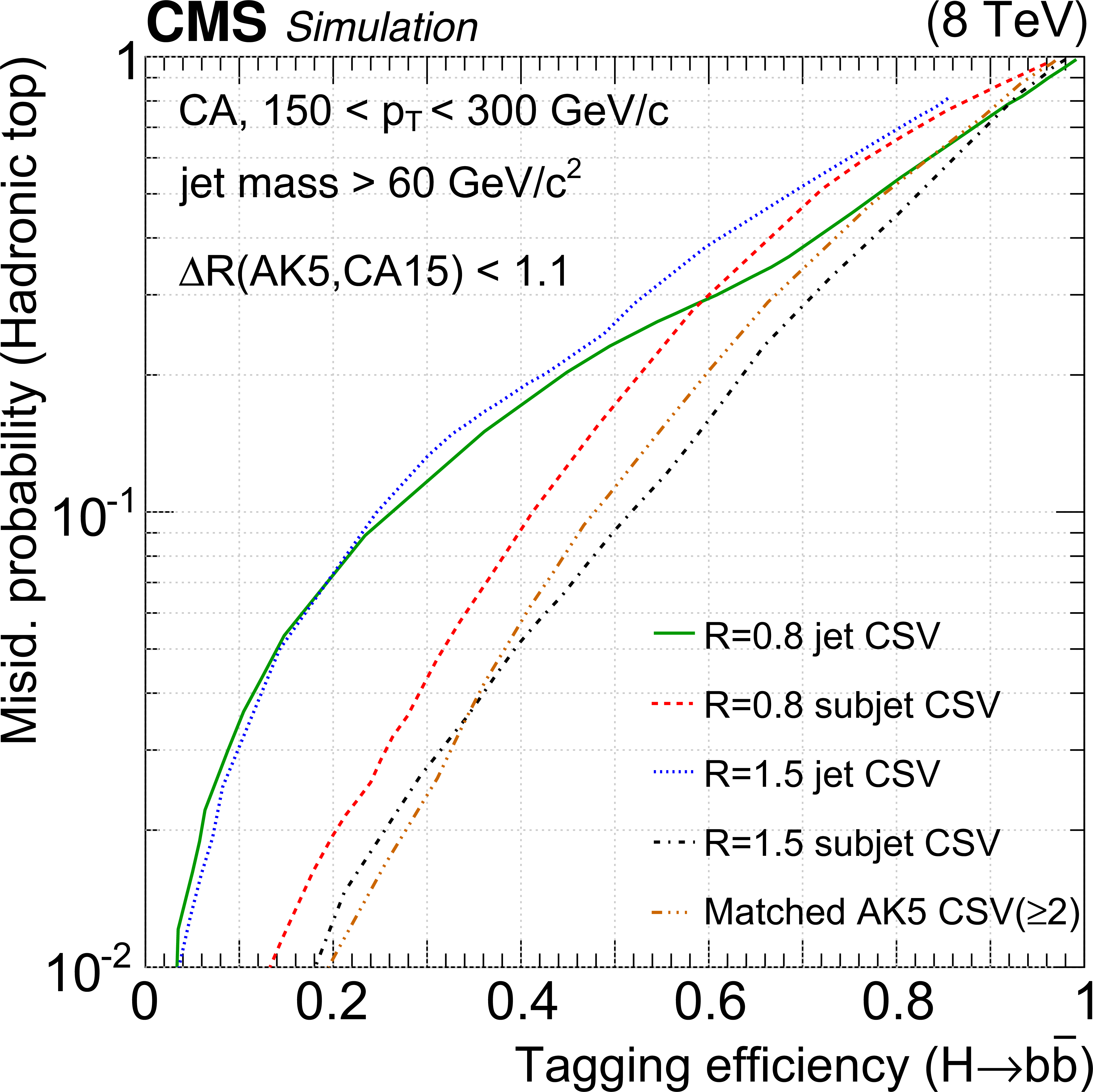
Figure 3-a:
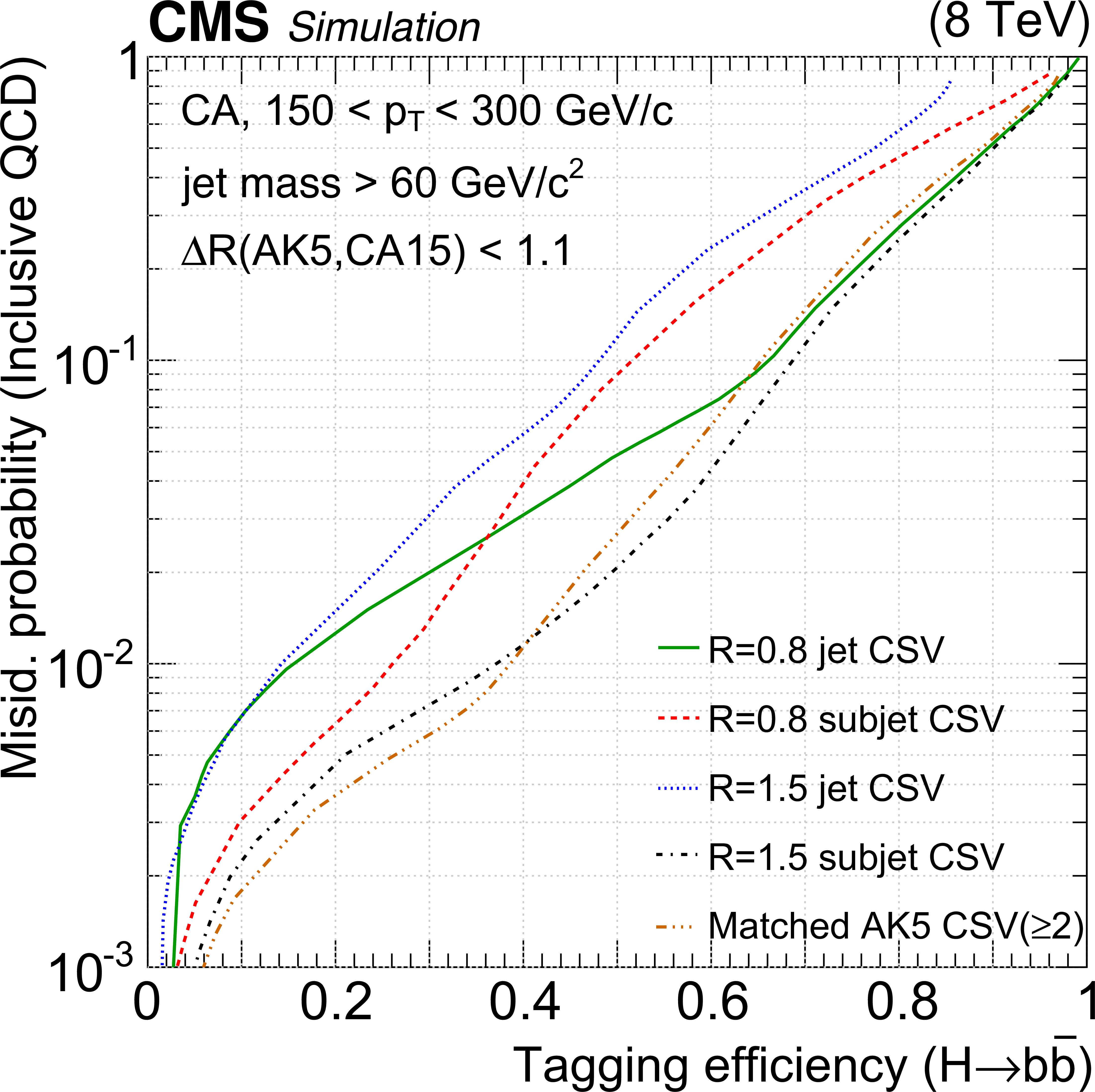
Performance of different H tagging algorithms in simulated signal events, with a signal mass hypothesis of 1000 GeV/$c^2$. The misidentification probability for inclusive QCD jets is shown versus the tagging efficiency for boosted Higgs boson decays, for jet transverse momentum ranges of (a) 150 $< {p_{\mathrm {T}}} <$ 300 GeV/$c$ and (b) 300 $< {p_{\mathrm {T}}} <$ 500 GeV/$c$. Different b tagging options are compared: standard b tagging of AK5 jets, subjet b tagging of CA15 and CA8 jets, and b tagging of CA15 jets and CA8 jets. For the case of subjet b tagging, two subjets are required to pass the b tagging criteria. Similarly, two AK5 jets are required to pass the b tagging criteria for standard b tagging. |
png pdf |
Figure 3-b:
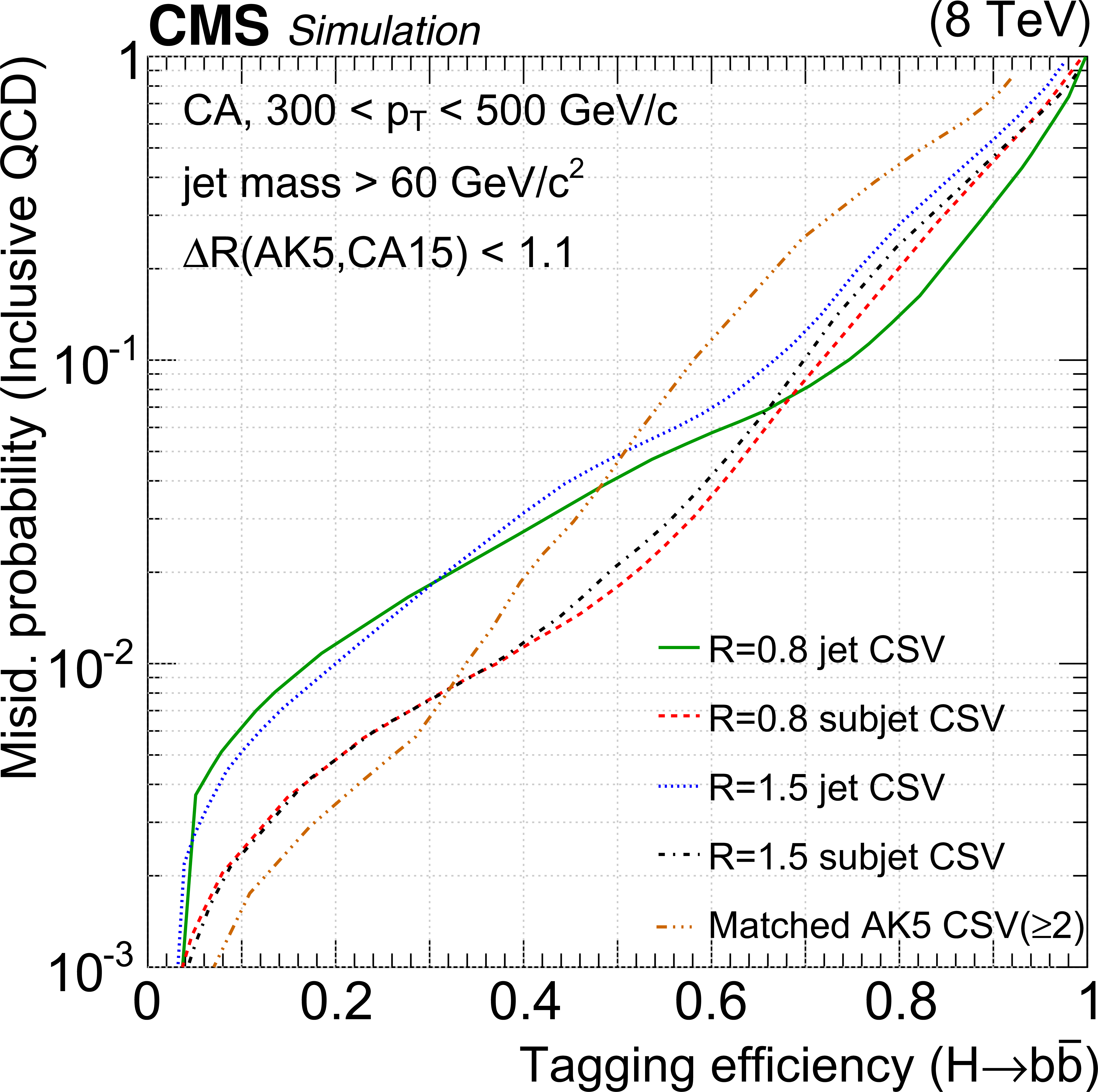
Performance of different H tagging algorithms in simulated signal events, with a signal mass hypothesis of 1000 GeV/$c^2$. The misidentification probability for inclusive QCD jets is shown versus the tagging efficiency for boosted Higgs boson decays, for jet transverse momentum ranges of (a) 150 $< {p_{\mathrm {T}}} <$ 300 GeV/$c$ and (b) 300 $< {p_{\mathrm {T}}} <$ 500 GeV/$c$. Different b tagging options are compared: standard b tagging of AK5 jets, subjet b tagging of CA15 and CA8 jets, and b tagging of CA15 jets and CA8 jets. For the case of subjet b tagging, two subjets are required to pass the b tagging criteria. Similarly, two AK5 jets are required to pass the b tagging criteria for standard b tagging. |
png pdf |
Figure 4-a:
Performance of different H tagging algorithms in simulated signal events, with a signal mass hypothesis of 1000 GeV/$c^2$. The misidentification probability for the $ {\mathrm {t}\overline {\mathrm {t}}} $ background is shown versus the tagging efficiency for boosted Higgs boson decays, for jet transverse momentum ranges of (a) 150 $< {p_{\mathrm {T}}} <$ 300 GeV/$c$ and (b) 300 $< {p_{\mathrm {T}}} <$ 500 GeV/$c$. Different b tagging options are compared: standard b tagging of AK5 jets, subjet b tagging of CA15 and CA8 jets, and b tagging of CA15 jets and CA8 jets. For the case of subjet b tagging, two subjets are required to pass the b tagging criteria. Similarly, two AK5 jets are required to pass the b tagging criteria for standard b tagging. |

png pdf |
Figure 4-b:
Performance of different H tagging algorithms in simulated signal events, with a signal mass hypothesis of 1000 GeV/$c^2$. The misidentification probability for the $ {\mathrm {t}\overline {\mathrm {t}}} $ background is shown versus the tagging efficiency for boosted Higgs boson decays, for jet transverse momentum ranges of (a) 150 $< {p_{\mathrm {T}}} <$ 300 GeV/$c$ and (b) 300 $< {p_{\mathrm {T}}} <$ 500 GeV/$c$. Different b tagging options are compared: standard b tagging of AK5 jets, subjet b tagging of CA15 and CA8 jets, and b tagging of CA15 jets and CA8 jets. For the case of subjet b tagging, two subjets are required to pass the b tagging criteria. Similarly, two AK5 jets are required to pass the b tagging criteria for standard b tagging. |
png pdf |
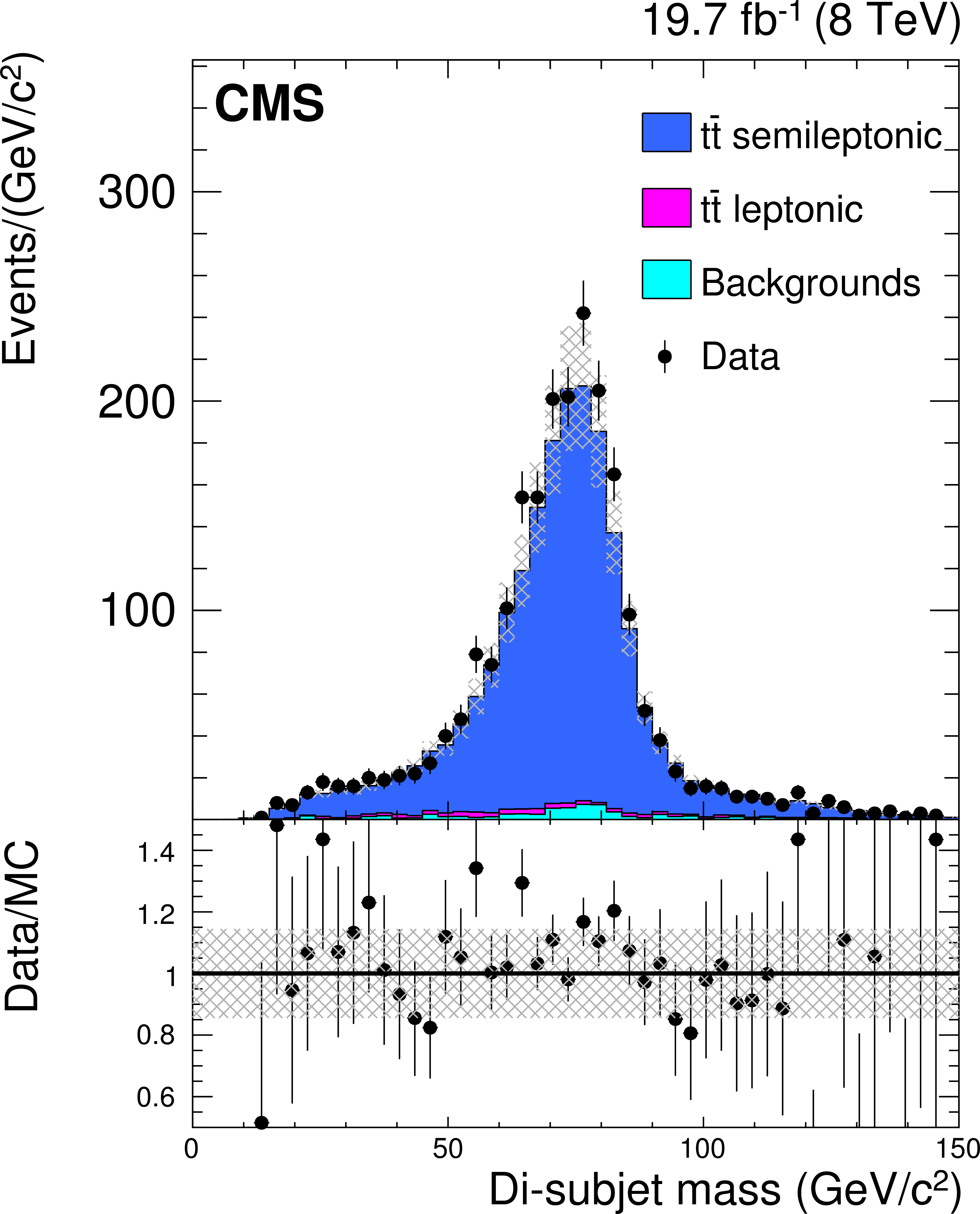
Figure 5:
Distribution of the invariant id-subjet mass of a hadronically decaying W boson obtained from a semi-leptonic $ {\mathrm {t}\overline {\mathrm {t}}} $ sample. The lower panel shows the ratio of data and simulation. The hatched area indicates the uncertainty in the signal and background cross sections. |
png pdf |
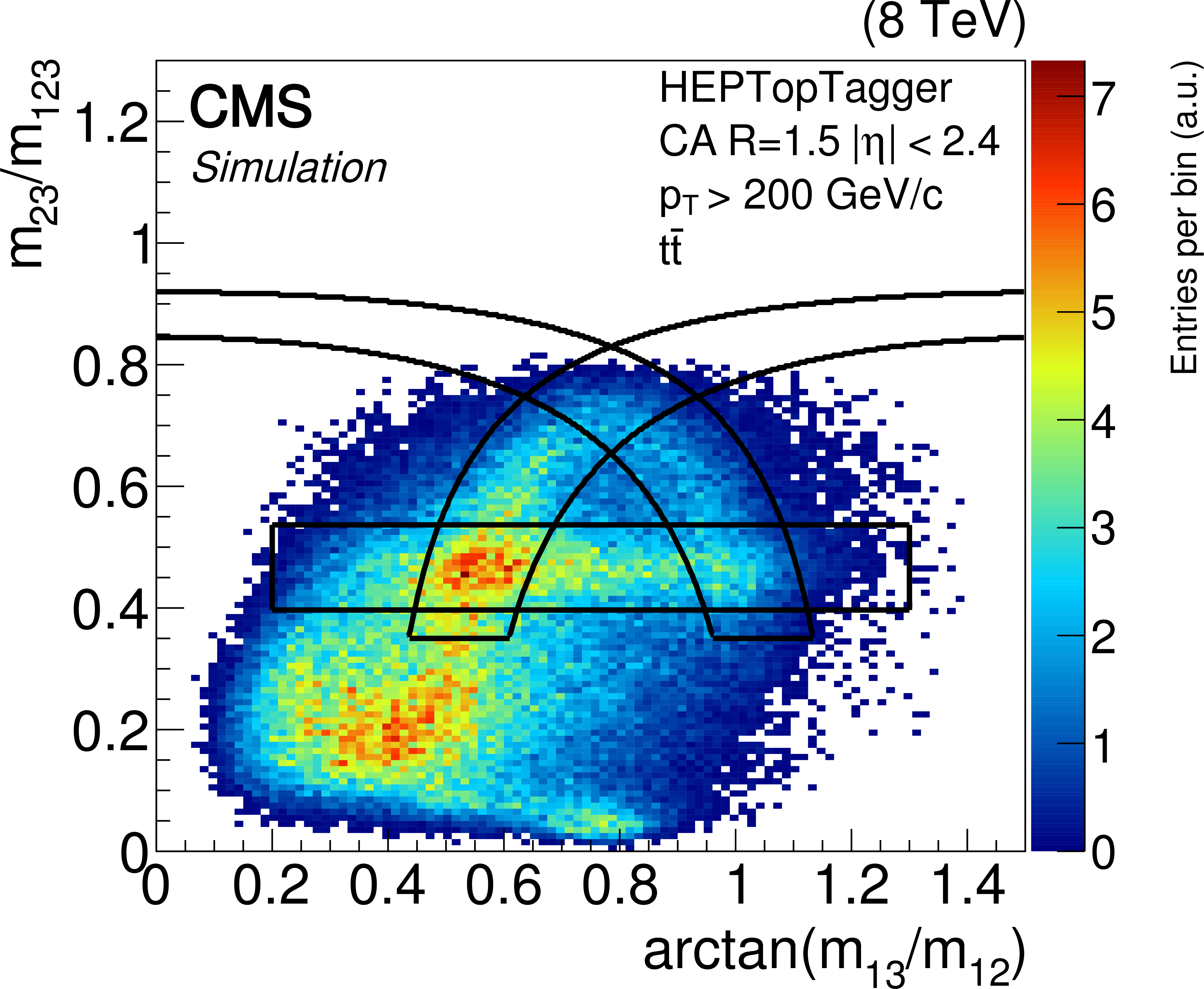
Figure 6-a:
Two-dimensional distributions of $m_{23}$/$m_{123}$ versus $\mathrm {arctan}(m_{13}/m_{12})$ for HEPTopTagger jets in simulated $ {\mathrm {t}\overline {\mathrm {t}}} $ events (a) and in simulated background events (b). The simulated background consists of boson+jets, di-boson, single-top, $ {\mathrm {t}\overline {\mathrm {t}}} $ all-hadronic, and $ {\mathrm {t}\overline {\mathrm {t}}} $ leptonic. The area enclosed by the thick solid lines denotes the region selected by the HEPTopTagger. |
png pdf |
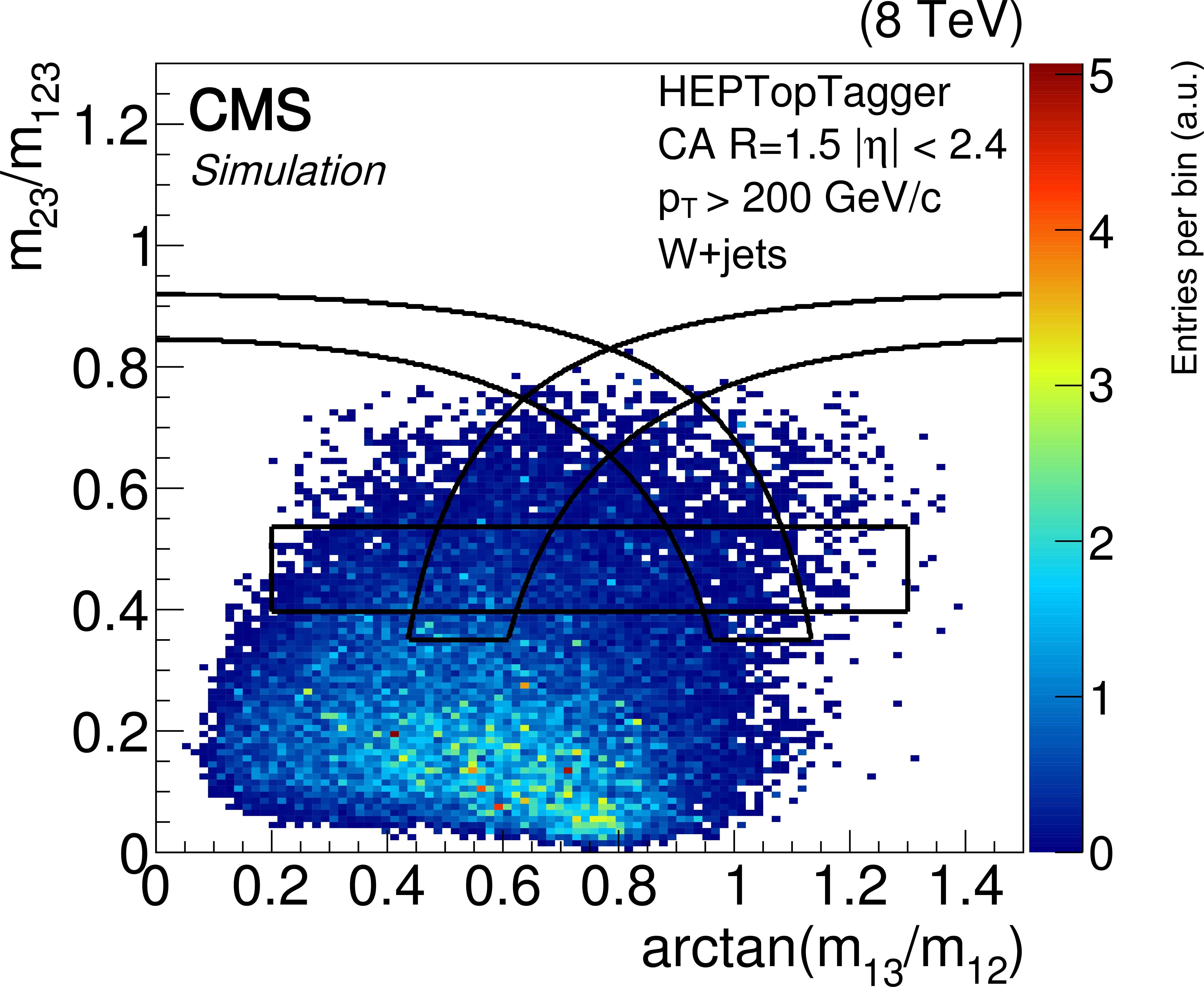
Figure 6-b:
Two-dimensional distributions of $m_{23}$/$m_{123}$ versus $\mathrm {arctan}(m_{13}/m_{12})$ for HEPTopTagger jets in simulated $ {\mathrm {t}\overline {\mathrm {t}}} $ events (a) and in simulated background events (b). The simulated background consists of boson+jets, di-boson, single-top, $ {\mathrm {t}\overline {\mathrm {t}}} $ all-hadronic, and $ {\mathrm {t}\overline {\mathrm {t}}} $ leptonic. The area enclosed by the thick solid lines denotes the region selected by the HEPTopTagger. |
png pdf |
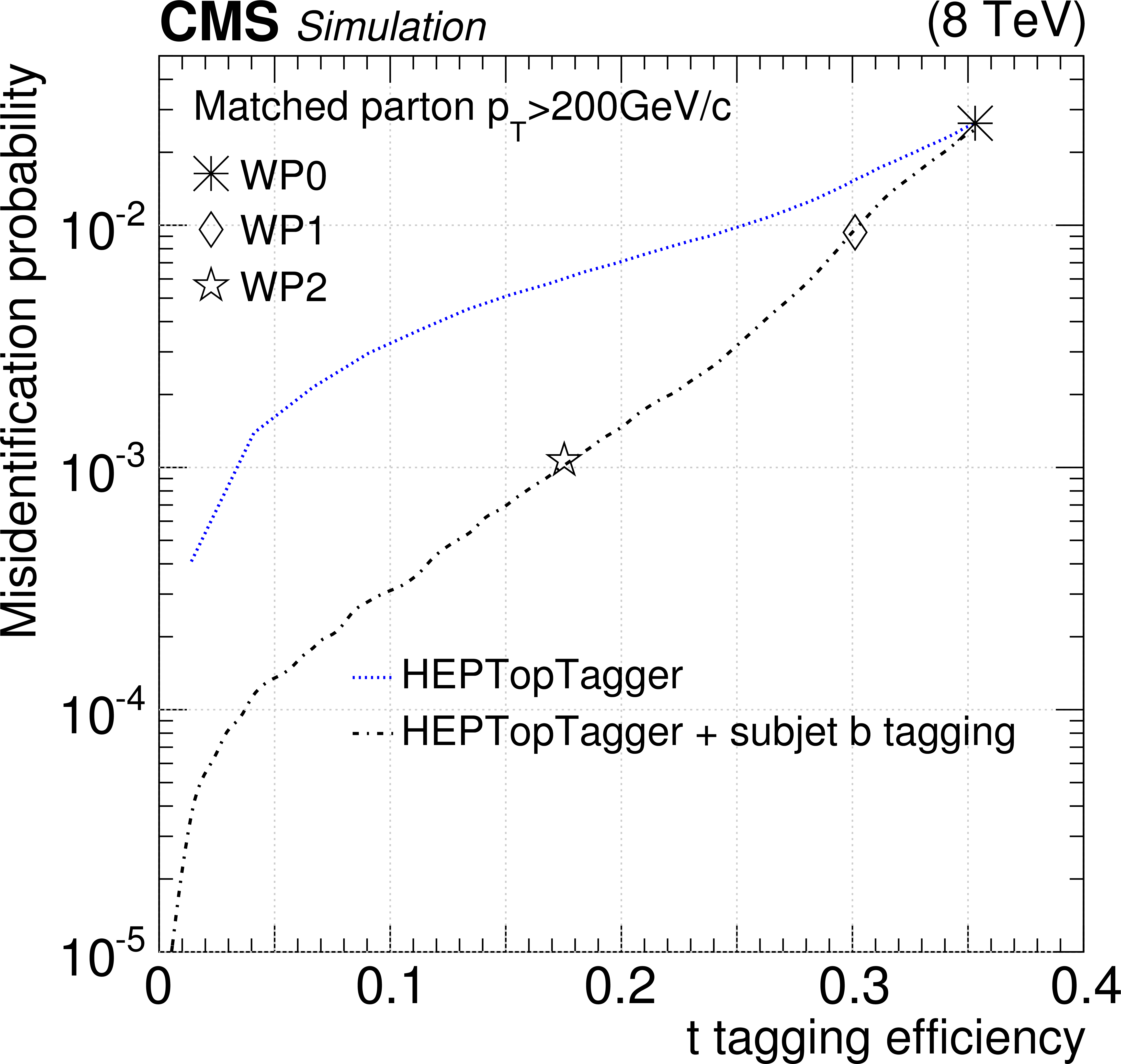
Figure 7:
Mistag rate versus t tagging efficiency for the HEPTopTagger and the combination of the HEPTopTagger with subjet b tagging, for CA15 jets matched to generated partons with $ {p_{\mathrm {T}}} > $ 200 GeV/$c$. The mistag rate is obtained from simulated QCD multijet events, while the efficiency is determined using simulated $ {\mathrm {t}\overline {\mathrm {t}}} $ events. |
png pdf |
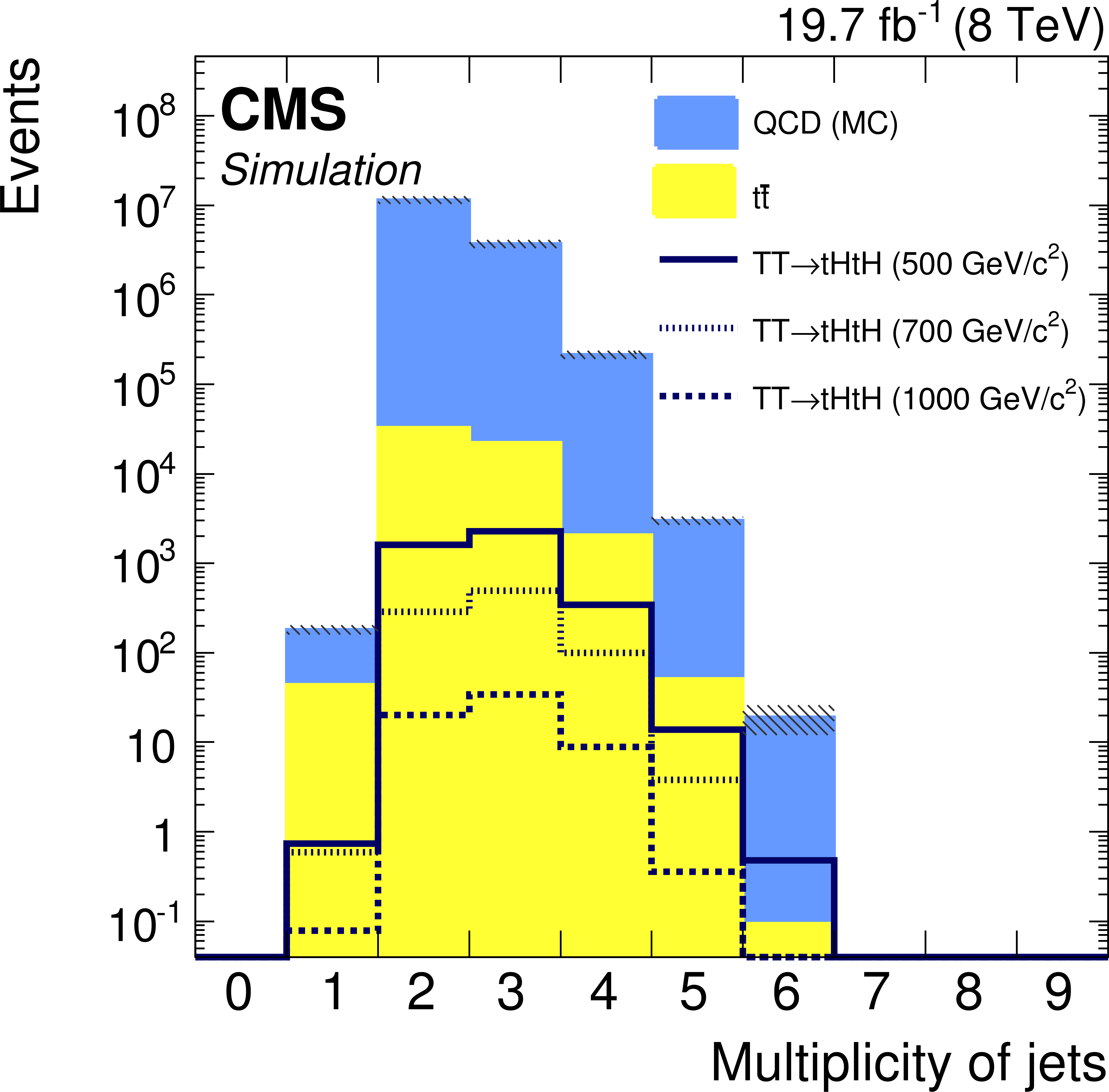
Figure 8-a:
a: multiplicity of CA15 jets with $ {p_{\mathrm {T}}} > $150 GeV/$c$. Events with at least two of these jets are selected. b: multiplicity of CA15 jets with $ {p_{\mathrm {T}}} > $ 200 GeV/$c$, that are selected by the HEPTopTagger algorithm. The solid histograms represent the simulated background processes ($ {\mathrm {t}\overline {\mathrm {t}}} $ and QCD multijet). The hatched error bands show the statistical uncertainty of the simulated events. |
png pdf |
Figure 8-b:
a: multiplicity of CA15 jets with $ {p_{\mathrm {T}}} > $150 GeV/$c$. Events with at least two of these jets are selected. b: multiplicity of CA15 jets with $ {p_{\mathrm {T}}} > $ 200 GeV/$c$, that are selected by the HEPTopTagger algorithm. The solid histograms represent the simulated background processes ($ {\mathrm {t}\overline {\mathrm {t}}} $ and QCD multijet). The hatched error bands show the statistical uncertainty of the simulated events. |

png pdf |
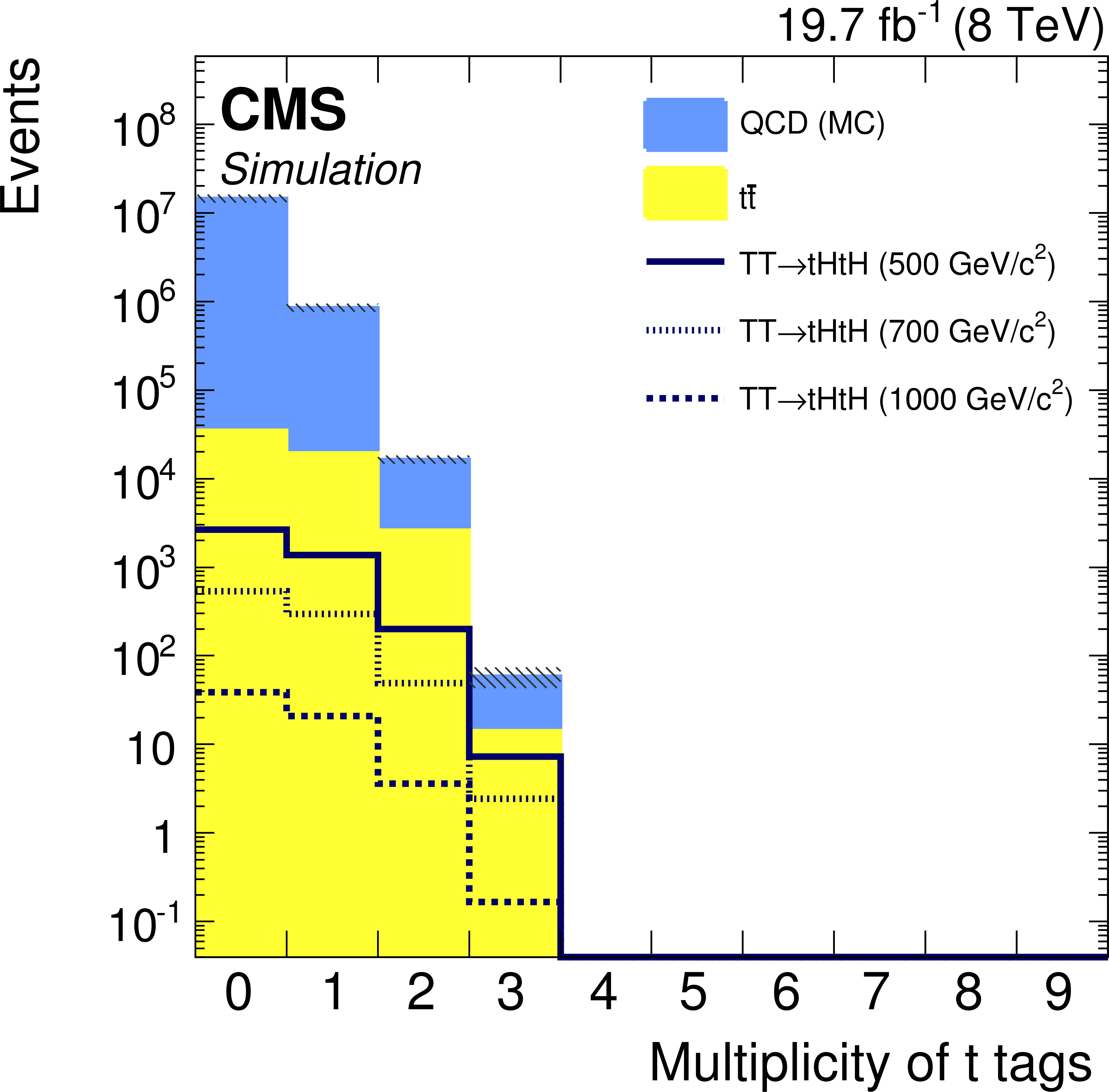
Figure 9-a:
a: multiplicity of CA15 jets with $ {p_{\mathrm {T}}} >$ 200 GeV/$c$ that are tagged by the HEPTopTagger and contain a b-tagged subjet, after requiring at least one jet per event to be selected by the HEPTopTagger algorithm. b: multiplicity of CA15 jets with $ {p_{\mathrm {T}}} > $150 GeV/$c$ satisfying the H tagging criteria. Events with three or more H tags are included in the bin with two H tags. The solid histograms represent the simulated background processes ($ {\mathrm {t}\overline {\mathrm {t}}} $ and QCD multijet). The hatched error bands show the statistical uncertainty of the simulated events. |
png pdf |
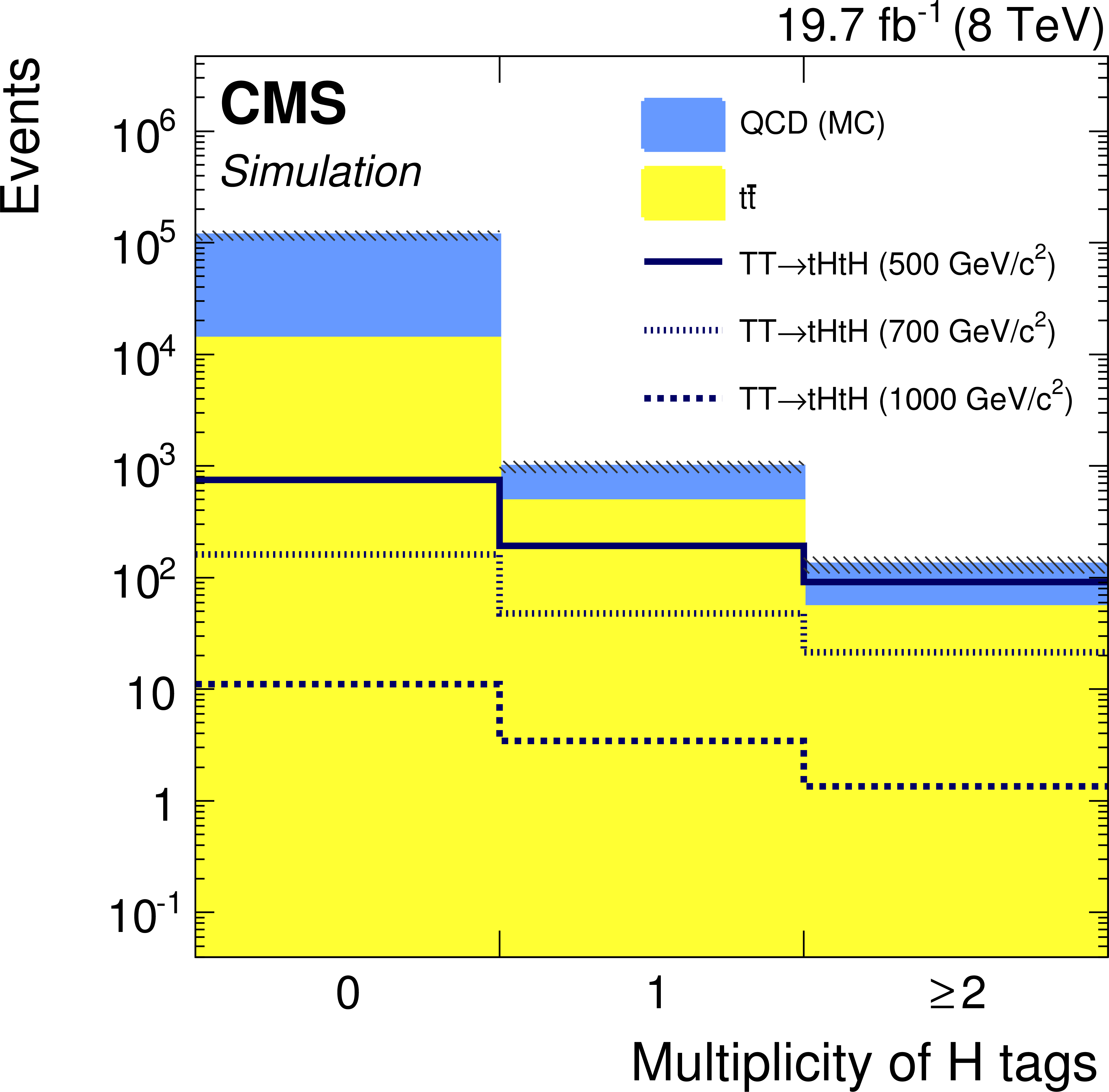
Figure 9-b:
a: multiplicity of CA15 jets with $ {p_{\mathrm {T}}} >$ 200 GeV/$c$ that are tagged by the HEPTopTagger and contain a b-tagged subjet, after requiring at least one jet per event to be selected by the HEPTopTagger algorithm. b: multiplicity of CA15 jets with $ {p_{\mathrm {T}}} > $150 GeV/$c$ satisfying the H tagging criteria. Events with three or more H tags are included in the bin with two H tags. The solid histograms represent the simulated background processes ($ {\mathrm {t}\overline {\mathrm {t}}} $ and QCD multijet). The hatched error bands show the statistical uncertainty of the simulated events. |

png pdf |
Figure 10-a:
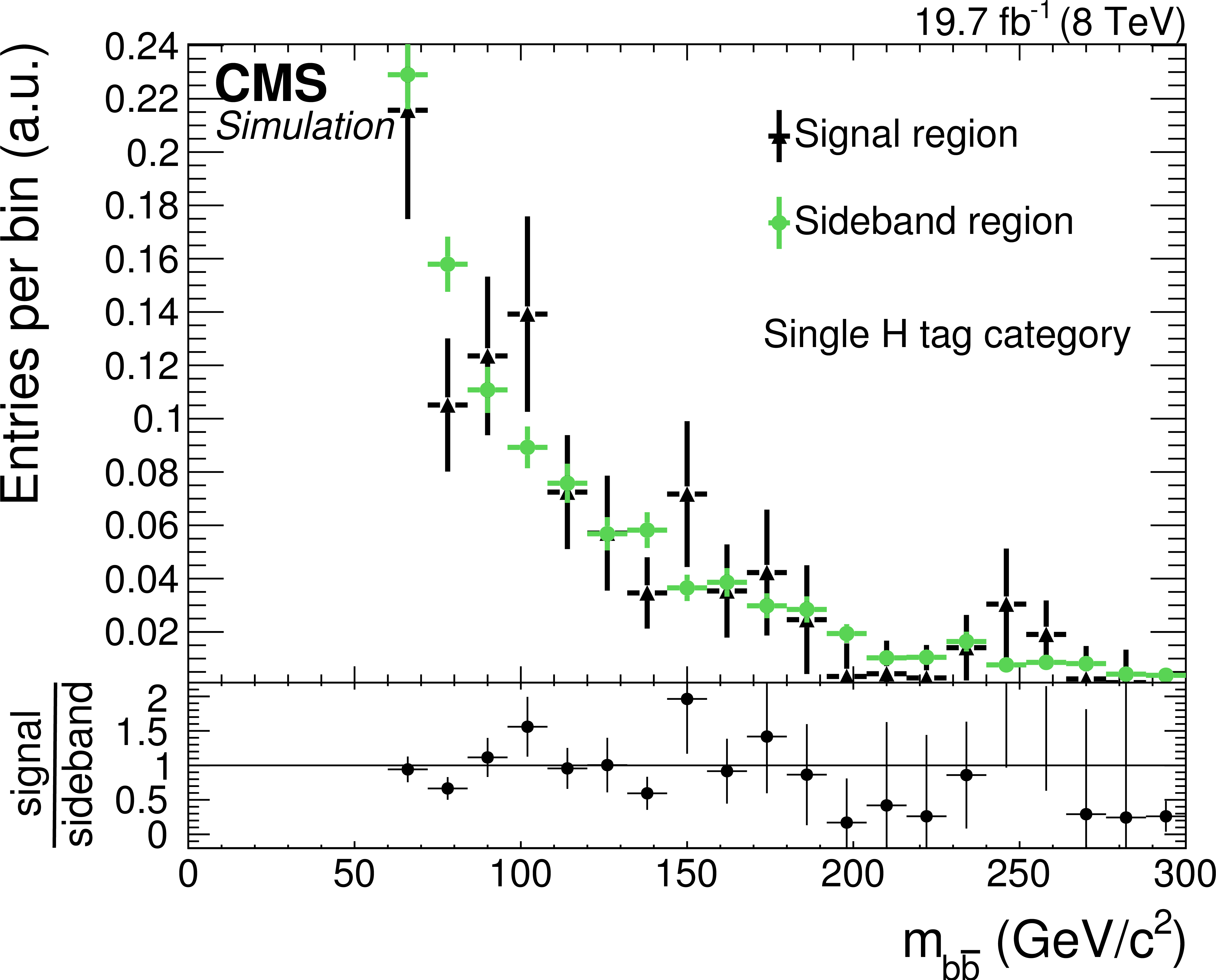
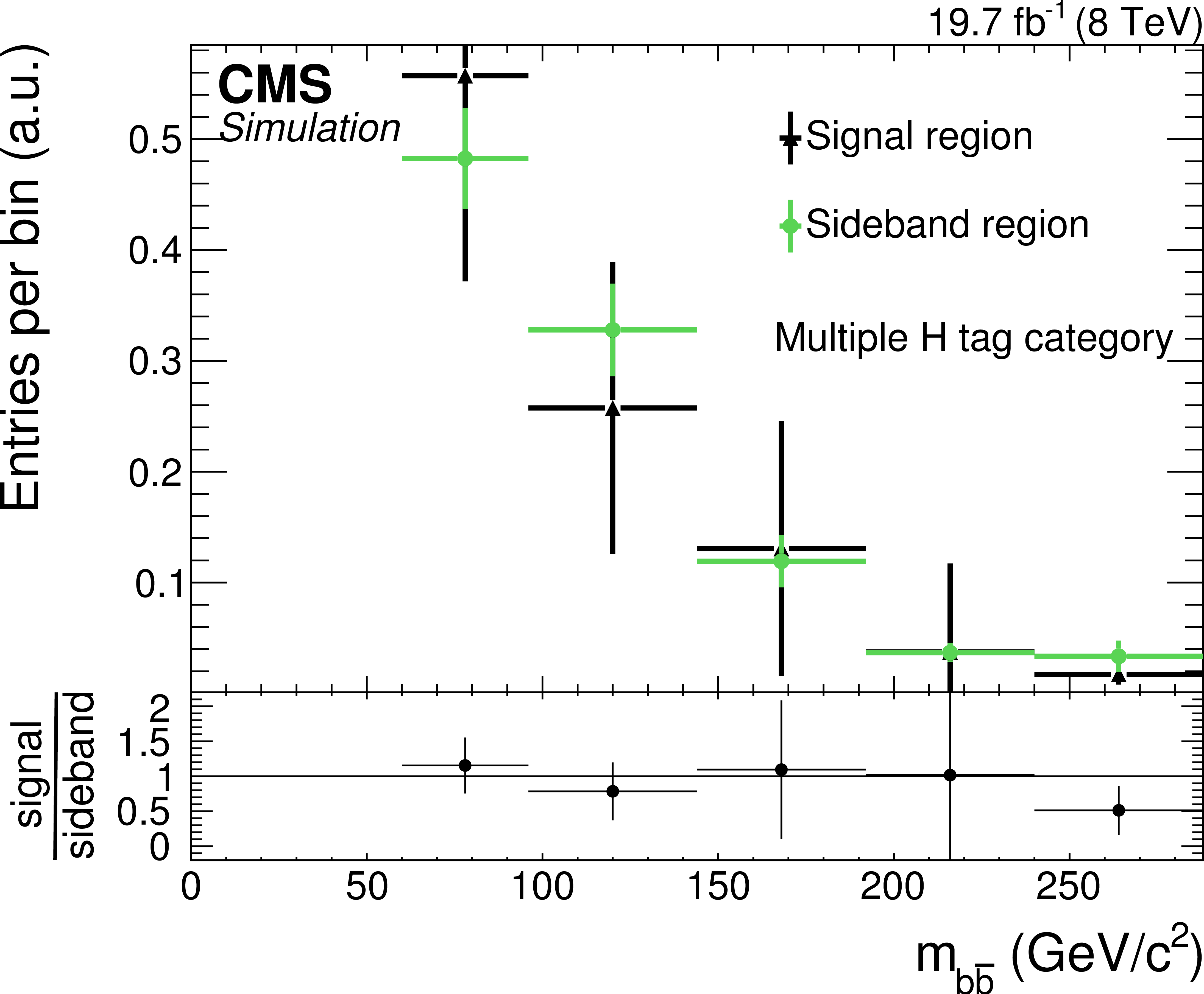
Comparison of the $ {H_{\mathrm {T}}} $ (a) and $m_{ { {\mathrm {b}} {\overline {\mathrm {b}}}} }$ (b) distributions in the sideband region B and signal region for the single (top) and multiple (c) H tag event categories for simulated QCD multijet events. All distributions are normalized to unity for shape comparison. The lower panels in the figures show the ratio of the signal and sideband regions. |
png pdf |
Figure 10-b:
Comparison of the $ {H_{\mathrm {T}}} $ (a) and $m_{ { {\mathrm {b}} {\overline {\mathrm {b}}}} }$ (b) distributions in the sideband region B and signal region for the single (top) and multiple (c) H tag event categories for simulated QCD multijet events. All distributions are normalized to unity for shape comparison. The lower panels in the figures show the ratio of the signal and sideband regions. |

png pdf |
Figure 10-c:
Comparison of the $ {H_{\mathrm {T}}} $ (a) and $m_{ { {\mathrm {b}} {\overline {\mathrm {b}}}} }$ (b) distributions in the sideband region B and signal region for the single (top) and multiple (c) H tag event categories for simulated QCD multijet events. All distributions are normalized to unity for shape comparison. The lower panels in the figures show the ratio of the signal and sideband regions. |
png pdf |
Figure 10-d:
Comparison of the $ {H_{\mathrm {T}}} $ (a) and $m_{ { {\mathrm {b}} {\overline {\mathrm {b}}}} }$ (b) distributions in the sideband region B and signal region for the single (top) and multiple (c) H tag event categories for simulated QCD multijet events. All distributions are normalized to unity for shape comparison. The lower panels in the figures show the ratio of the signal and sideband regions. |
png pdf |
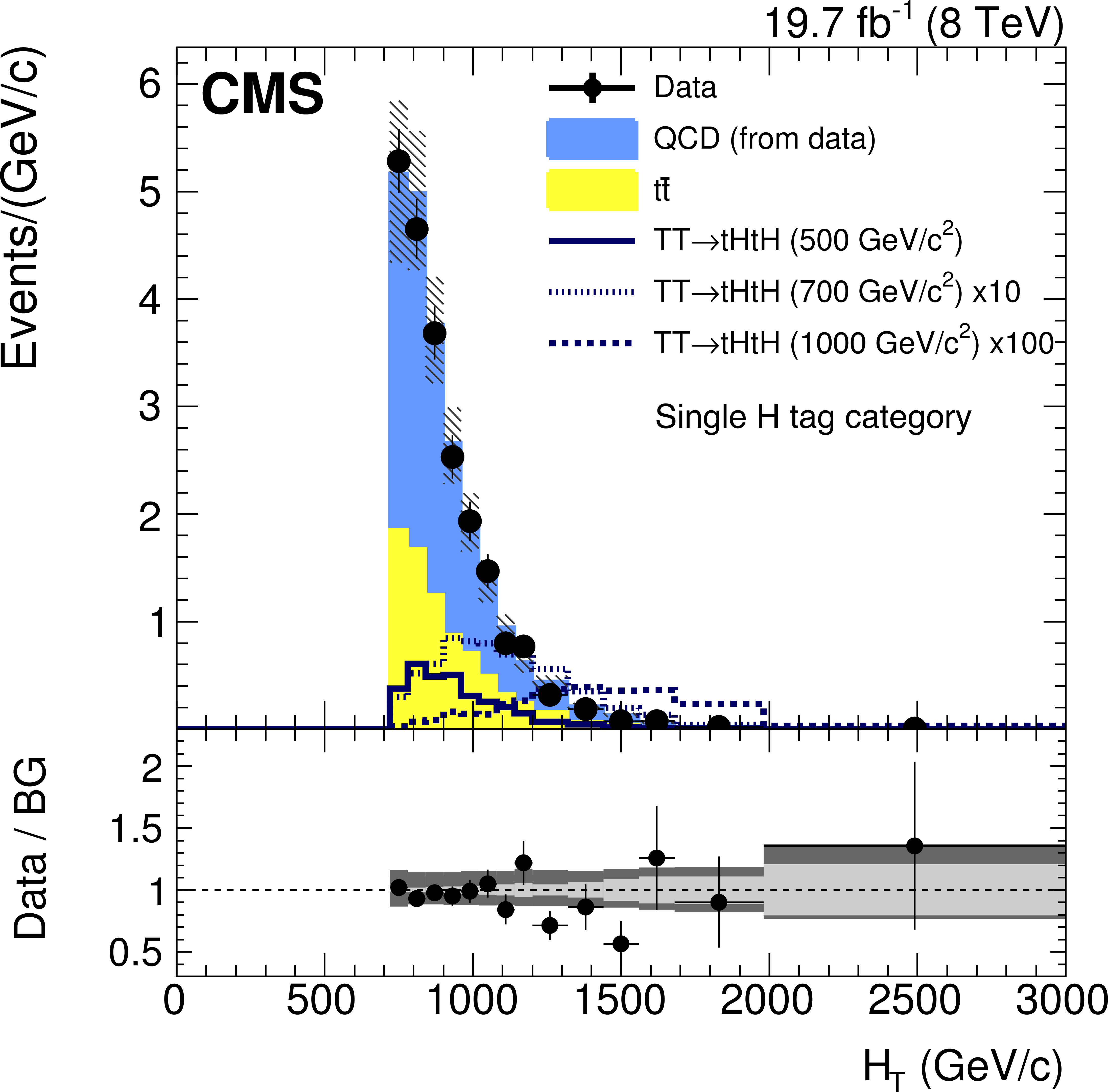
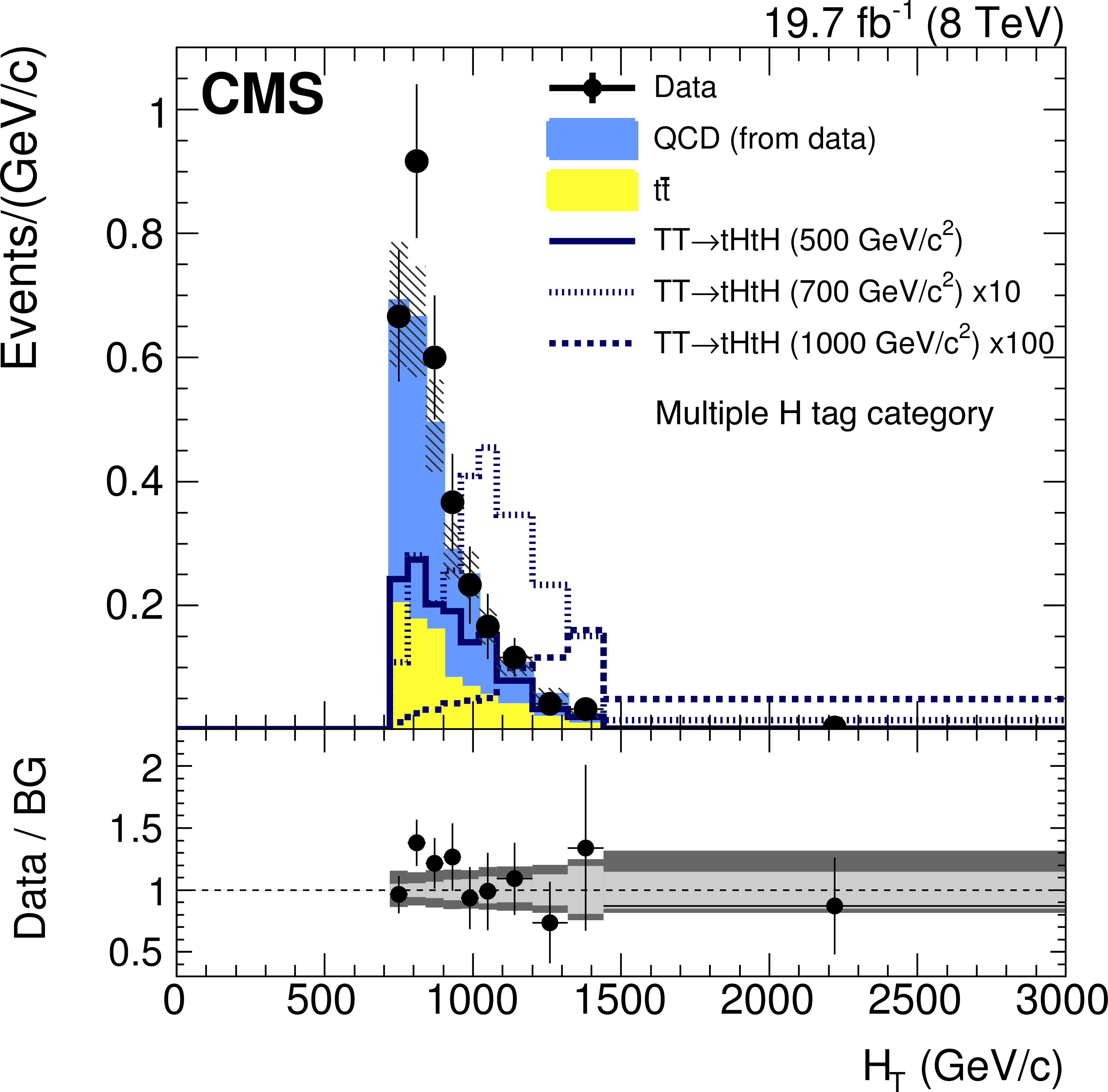
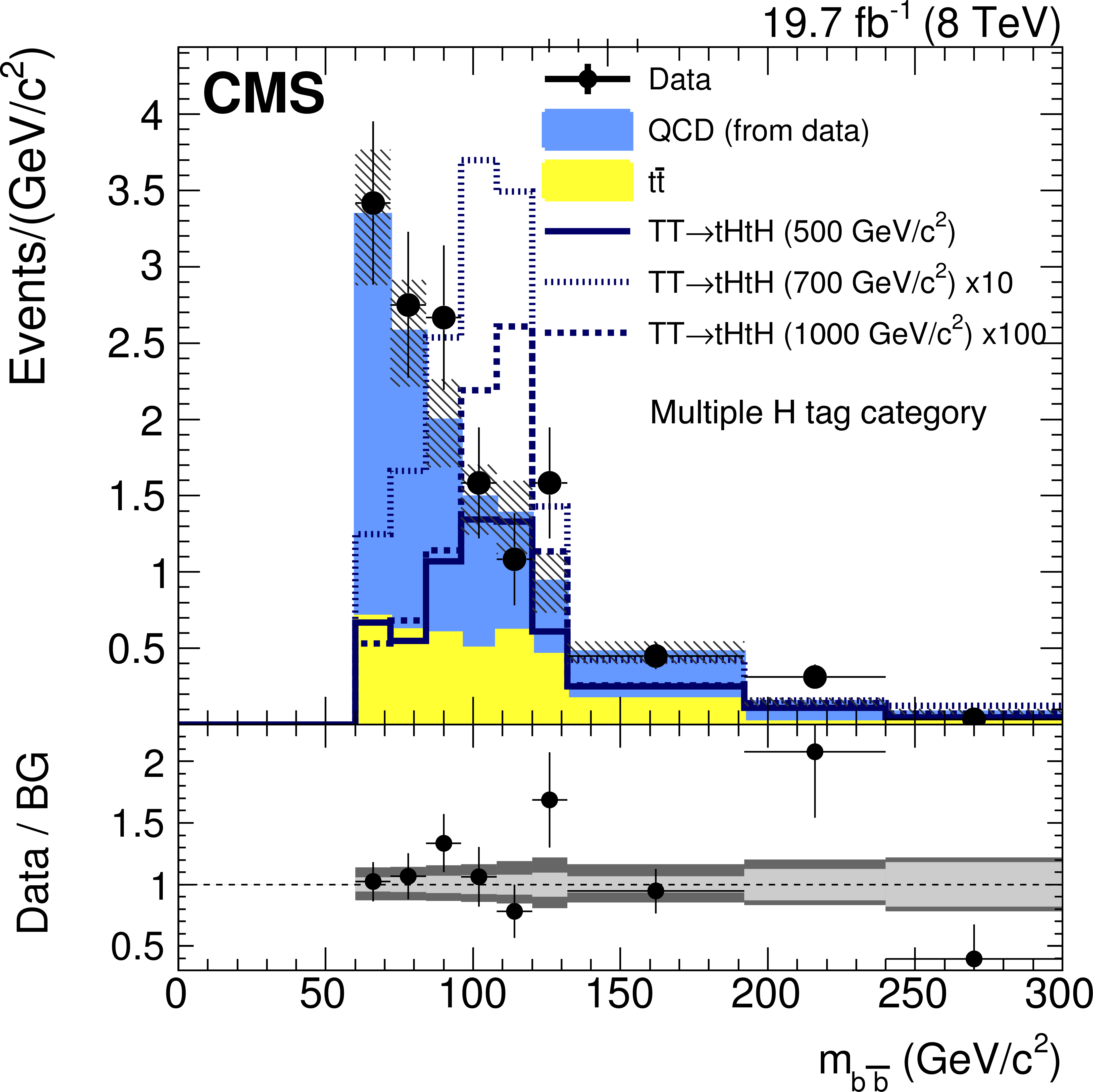
Figure 11-a:
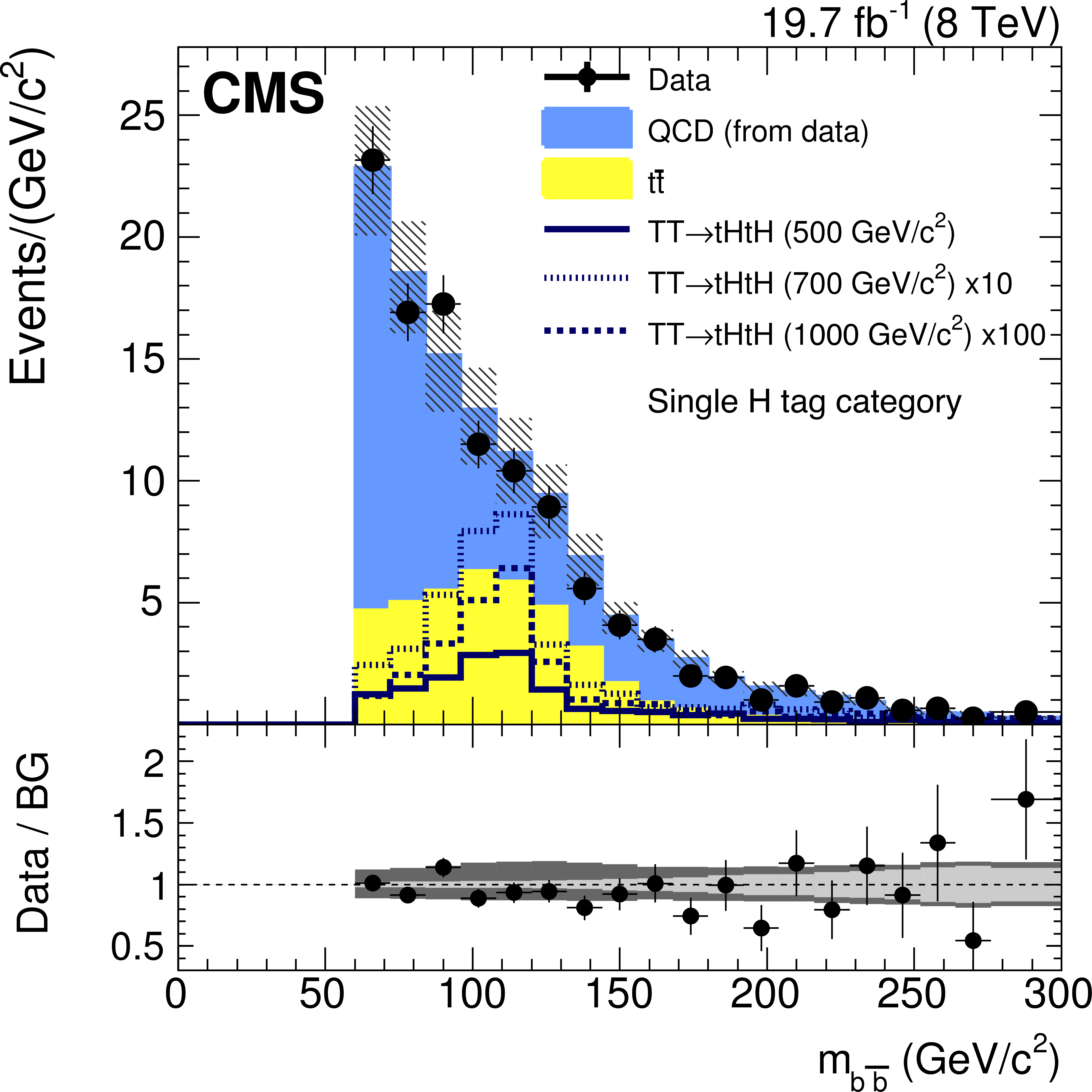
The $ {H_{\mathrm {T}}} $ (a, c) and Higgs boson candidate mass (b, d) distributions for the single H tag category (a, b) and the multiple H tag category (c, d). The QCD multijet background is derived from data. The $ {\mathrm {t}\overline {\mathrm {t}}} $ background is taken from simulation. The hypothetical signal is shown for three different mass points: 500, 700, and 1000 GeV/$c^2$. The hatched error bands show the quadratic sum of all systematic and statistical uncertainties in the background. In the ratio plot, the statistical uncertainty in the background is depicted by the inner central band, while the outer band shows the quadratic sum of all systematic and statistical uncertainties. |
png pdf |
Figure 11-b:
The $ {H_{\mathrm {T}}} $ (a, c) and Higgs boson candidate mass (b, d) distributions for the single H tag category (a, b) and the multiple H tag category (c, d). The QCD multijet background is derived from data. The $ {\mathrm {t}\overline {\mathrm {t}}} $ background is taken from simulation. The hypothetical signal is shown for three different mass points: 500, 700, and 1000 GeV/$c^2$. The hatched error bands show the quadratic sum of all systematic and statistical uncertainties in the background. In the ratio plot, the statistical uncertainty in the background is depicted by the inner central band, while the outer band shows the quadratic sum of all systematic and statistical uncertainties. |
png pdf |
Figure 11-c:
The $ {H_{\mathrm {T}}} $ (a, c) and Higgs boson candidate mass (b, d) distributions for the single H tag category (a, b) and the multiple H tag category (c, d). The QCD multijet background is derived from data. The $ {\mathrm {t}\overline {\mathrm {t}}} $ background is taken from simulation. The hypothetical signal is shown for three different mass points: 500, 700, and 1000 GeV/$c^2$. The hatched error bands show the quadratic sum of all systematic and statistical uncertainties in the background. In the ratio plot, the statistical uncertainty in the background is depicted by the inner central band, while the outer band shows the quadratic sum of all systematic and statistical uncertainties. |
png pdf |
Figure 11-d:
The $ {H_{\mathrm {T}}} $ (a, c) and Higgs boson candidate mass (b, d) distributions for the single H tag category (a, b) and the multiple H tag category (c, d). The QCD multijet background is derived from data. The $ {\mathrm {t}\overline {\mathrm {t}}} $ background is taken from simulation. The hypothetical signal is shown for three different mass points: 500, 700, and 1000 GeV/$c^2$. The hatched error bands show the quadratic sum of all systematic and statistical uncertainties in the background. In the ratio plot, the statistical uncertainty in the background is depicted by the inner central band, while the outer band shows the quadratic sum of all systematic and statistical uncertainties. |
png pdf |
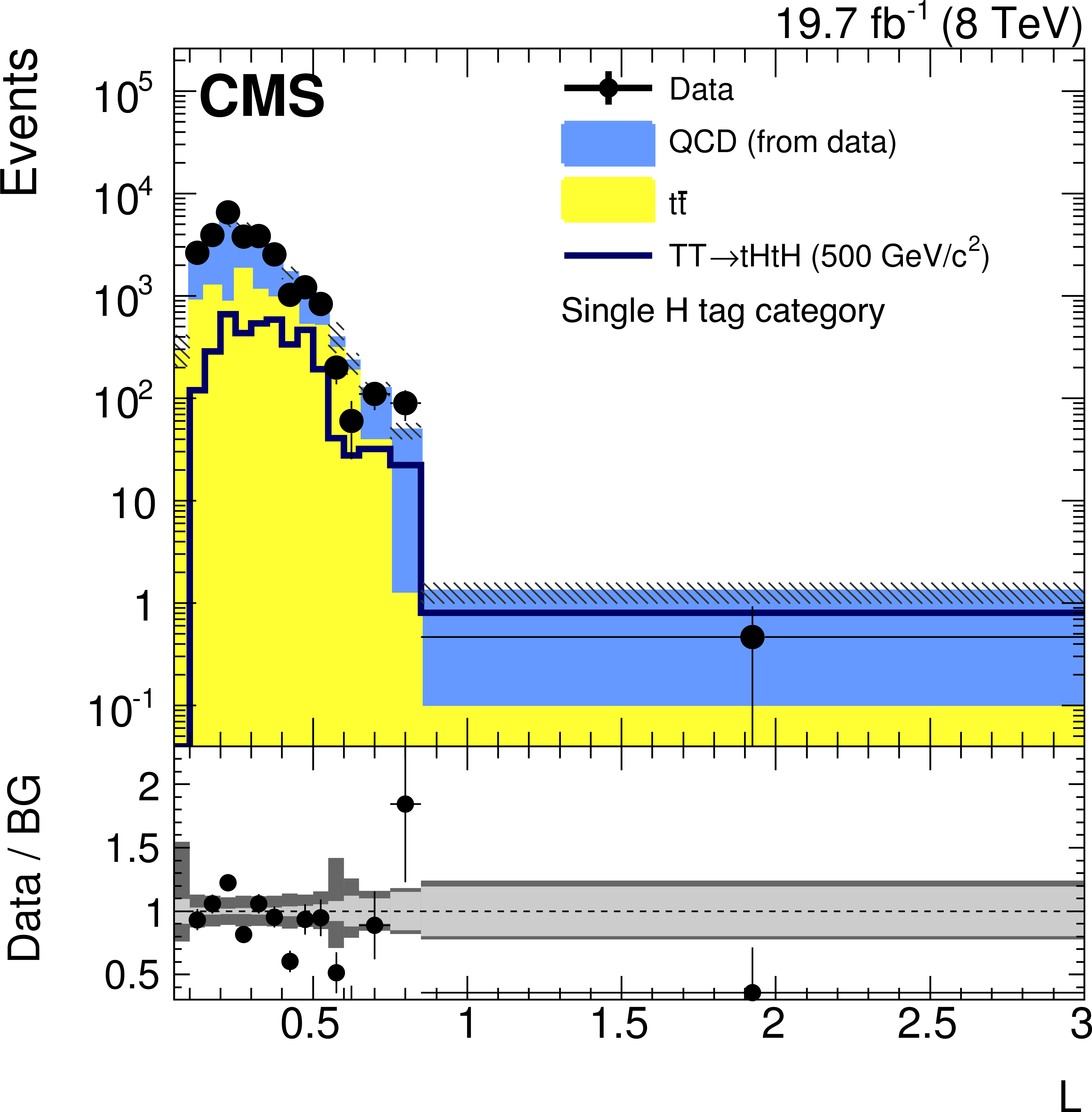
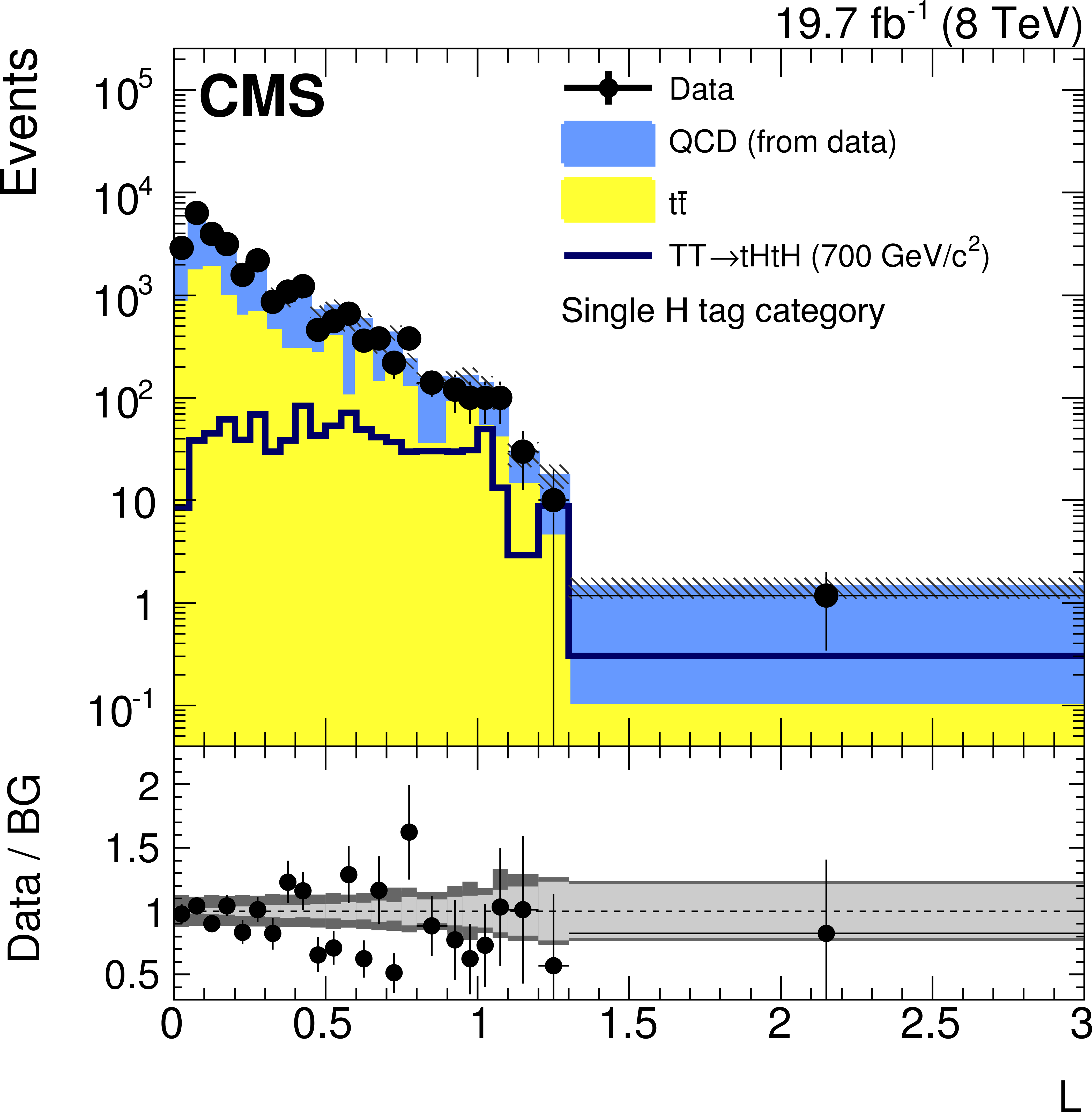
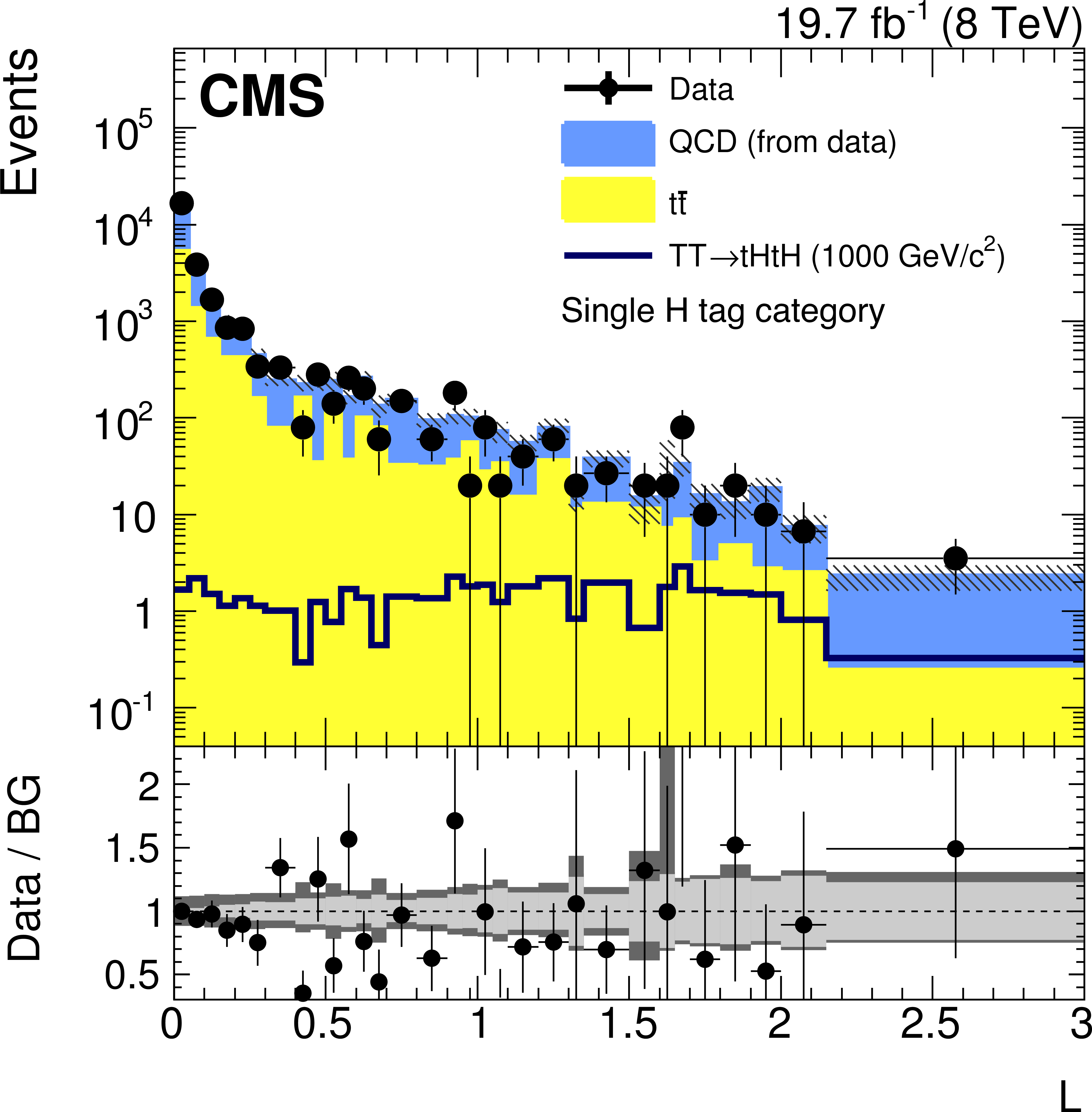
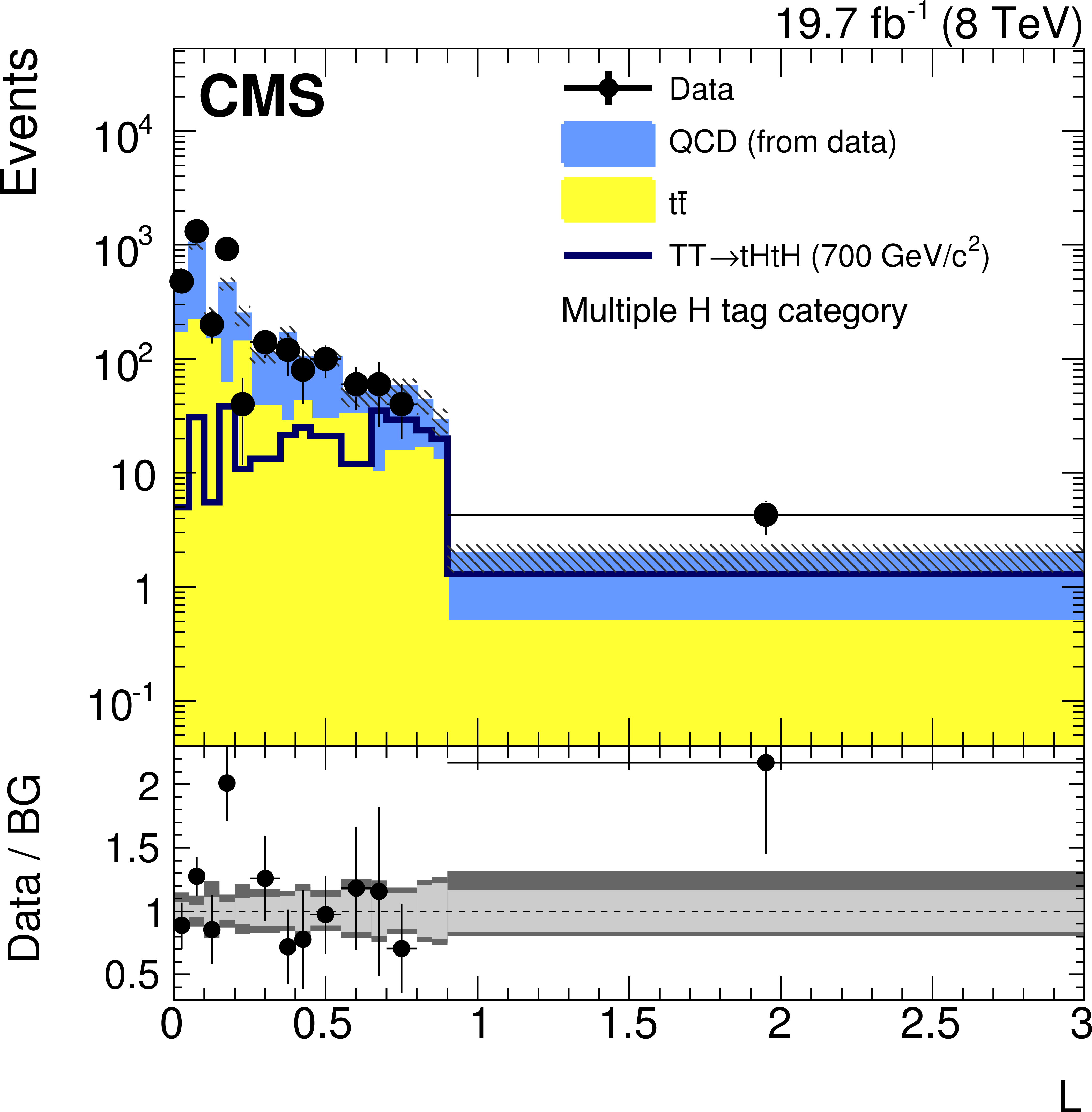
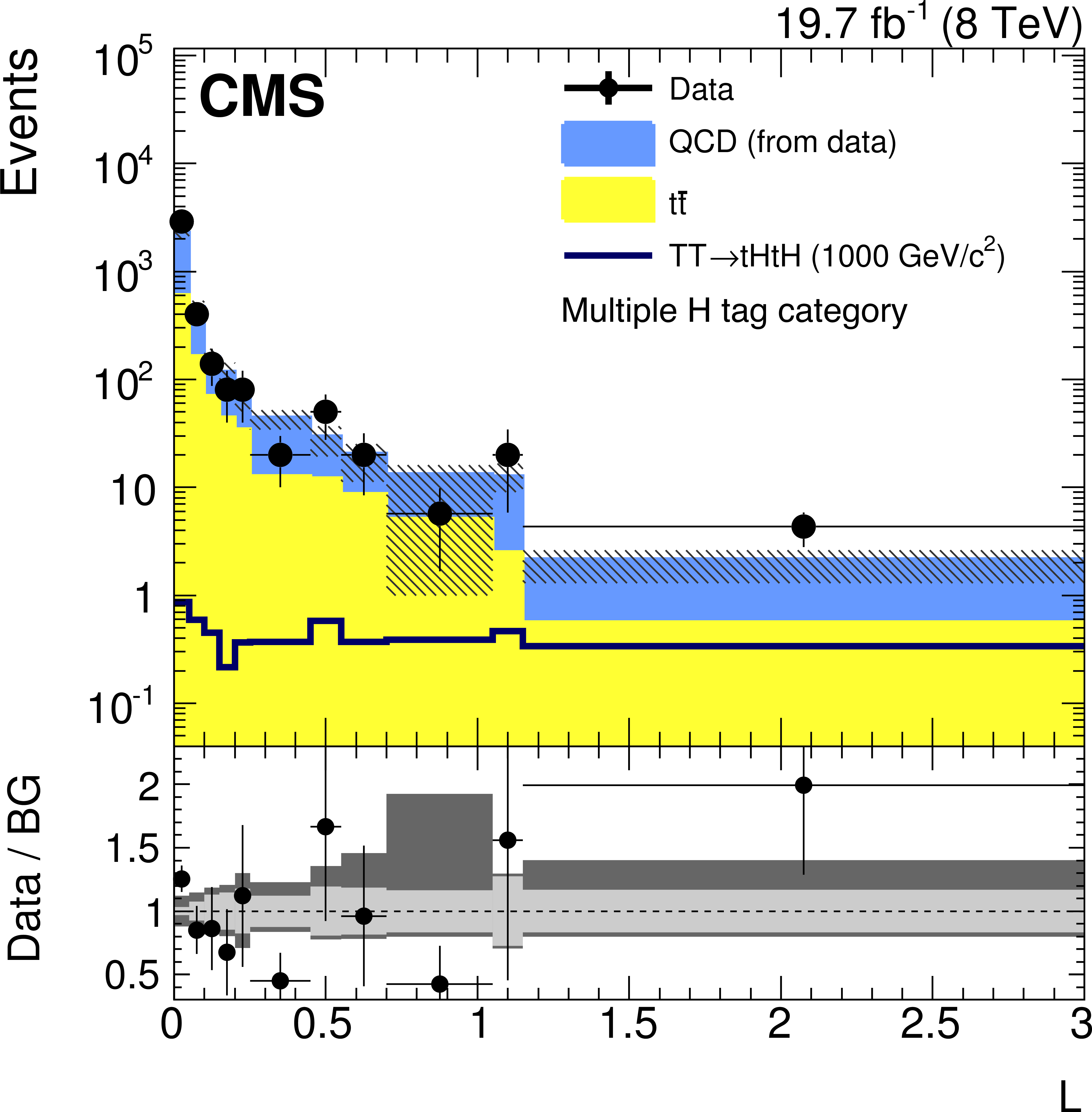
Figure 12-a:
Discriminating variable $L$ constructed from both $ {H_{\mathrm {T}}} $ and $m_{ { {\mathrm {b}} {\overline {\mathrm {b}}}} }$ for the single (a, b, c) and the multiple (d, e, f) H tag categories. The three signal hypotheses with 500, 700, and 1000 GeV/$c^2$ are shown on (a, d), (b, e), and (c, f), respectively. The QCD multijet background is derived from data. The $ {\mathrm {t}\overline {\mathrm {t}}} $ background is derived from simulation. The hatched error bands show the quadratic sum of all systematic and statistical uncertainties in the background. In the ratio plot, the statistical uncertainty in the background is depicted by the inner central band, while the outer band shows the quadratic sum of all systematic and statistical uncertainties. |
png pdf |
Figure 12-b:
Discriminating variable $L$ constructed from both $ {H_{\mathrm {T}}} $ and $m_{ { {\mathrm {b}} {\overline {\mathrm {b}}}} }$ for the single (a, b, c) and the multiple (d, e, f) H tag categories. The three signal hypotheses with 500, 700, and 1000 GeV/$c^2$ are shown on (a, d), (b, e), and (c, f), respectively. The QCD multijet background is derived from data. The $ {\mathrm {t}\overline {\mathrm {t}}} $ background is derived from simulation. The hatched error bands show the quadratic sum of all systematic and statistical uncertainties in the background. In the ratio plot, the statistical uncertainty in the background is depicted by the inner central band, while the outer band shows the quadratic sum of all systematic and statistical uncertainties. |
png pdf |
Figure 12-c:
Discriminating variable $L$ constructed from both $ {H_{\mathrm {T}}} $ and $m_{ { {\mathrm {b}} {\overline {\mathrm {b}}}} }$ for the single (a, b, c) and the multiple (d, e, f) H tag categories. The three signal hypotheses with 500, 700, and 1000 GeV/$c^2$ are shown on (a, d), (b, e), and (c, f), respectively. The QCD multijet background is derived from data. The $ {\mathrm {t}\overline {\mathrm {t}}} $ background is derived from simulation. The hatched error bands show the quadratic sum of all systematic and statistical uncertainties in the background. In the ratio plot, the statistical uncertainty in the background is depicted by the inner central band, while the outer band shows the quadratic sum of all systematic and statistical uncertainties. |

png pdf |
Figure 12-d:
Discriminating variable $L$ constructed from both $ {H_{\mathrm {T}}} $ and $m_{ { {\mathrm {b}} {\overline {\mathrm {b}}}} }$ for the single (a, b, c) and the multiple (d, e, f) H tag categories. The three signal hypotheses with 500, 700, and 1000 GeV/$c^2$ are shown on (a, d), (b, e), and (c, f), respectively. The QCD multijet background is derived from data. The $ {\mathrm {t}\overline {\mathrm {t}}} $ background is derived from simulation. The hatched error bands show the quadratic sum of all systematic and statistical uncertainties in the background. In the ratio plot, the statistical uncertainty in the background is depicted by the inner central band, while the outer band shows the quadratic sum of all systematic and statistical uncertainties. |
png pdf |
Figure 12-e:
Discriminating variable $L$ constructed from both $ {H_{\mathrm {T}}} $ and $m_{ { {\mathrm {b}} {\overline {\mathrm {b}}}} }$ for the single (a, b, c) and the multiple (d, e, f) H tag categories. The three signal hypotheses with 500, 700, and 1000 GeV/$c^2$ are shown on (a, d), (b, e), and (c, f), respectively. The QCD multijet background is derived from data. The $ {\mathrm {t}\overline {\mathrm {t}}} $ background is derived from simulation. The hatched error bands show the quadratic sum of all systematic and statistical uncertainties in the background. In the ratio plot, the statistical uncertainty in the background is depicted by the inner central band, while the outer band shows the quadratic sum of all systematic and statistical uncertainties. |
png pdf |
Figure 12-f:
Discriminating variable $L$ constructed from both $ {H_{\mathrm {T}}} $ and $m_{ { {\mathrm {b}} {\overline {\mathrm {b}}}} }$ for the single (a, b, c) and the multiple (d, e, f) H tag categories. The three signal hypotheses with 500, 700, and 1000 GeV/$c^2$ are shown on (a, d), (b, e), and (c, f), respectively. The QCD multijet background is derived from data. The $ {\mathrm {t}\overline {\mathrm {t}}} $ background is derived from simulation. The hatched error bands show the quadratic sum of all systematic and statistical uncertainties in the background. In the ratio plot, the statistical uncertainty in the background is depicted by the inner central band, while the outer band shows the quadratic sum of all systematic and statistical uncertainties. |
png pdf |
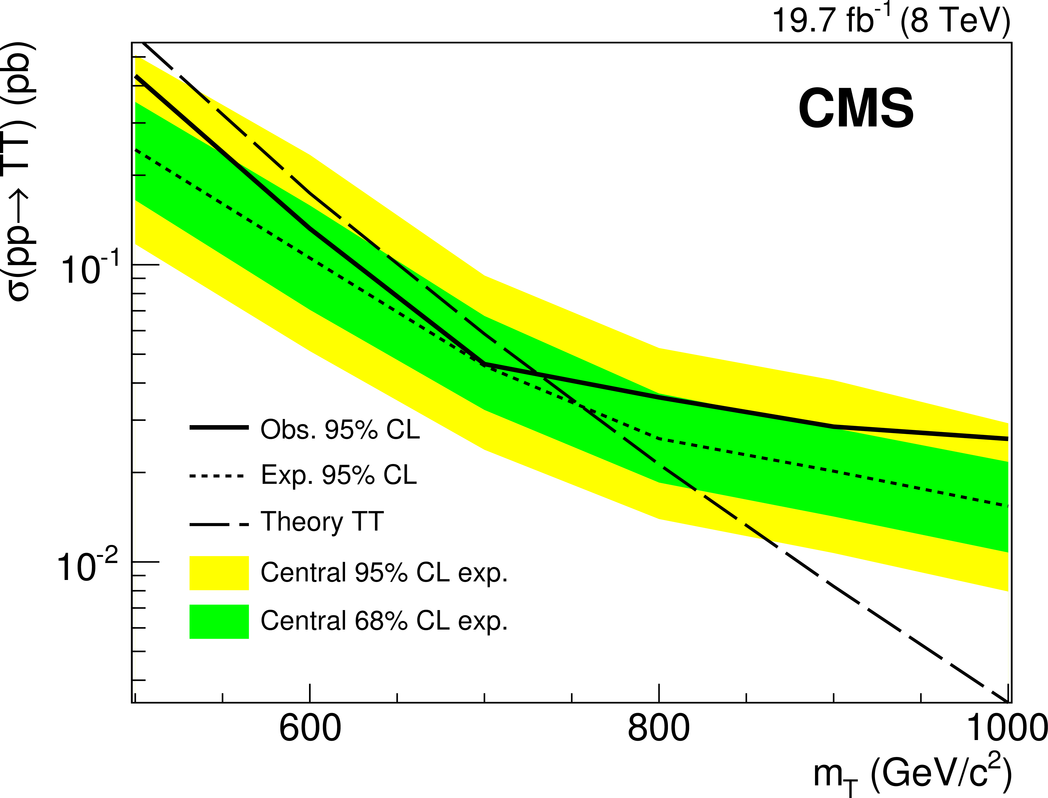
Figure 13:
Observed (solid line) and expected (dotted line) Bayesian upper limits on the T quark production cross section determined from the variable $L$ for the combination of the single and multiple H tag categories, for the hypothesis of an exclusive branching fraction $\mathcal {B}( {\mathrm {T}} \to {\mathrm {t}} {\mathrm {H}} )$ = 100%. The green (inner) and yellow (outer) bands show the $1\sigma $ ($2\sigma $) uncertainty ranges, respectively. The dashed line shows the prediction of the theory as discussed in Section \ref {sec:samples}. |
png pdf |
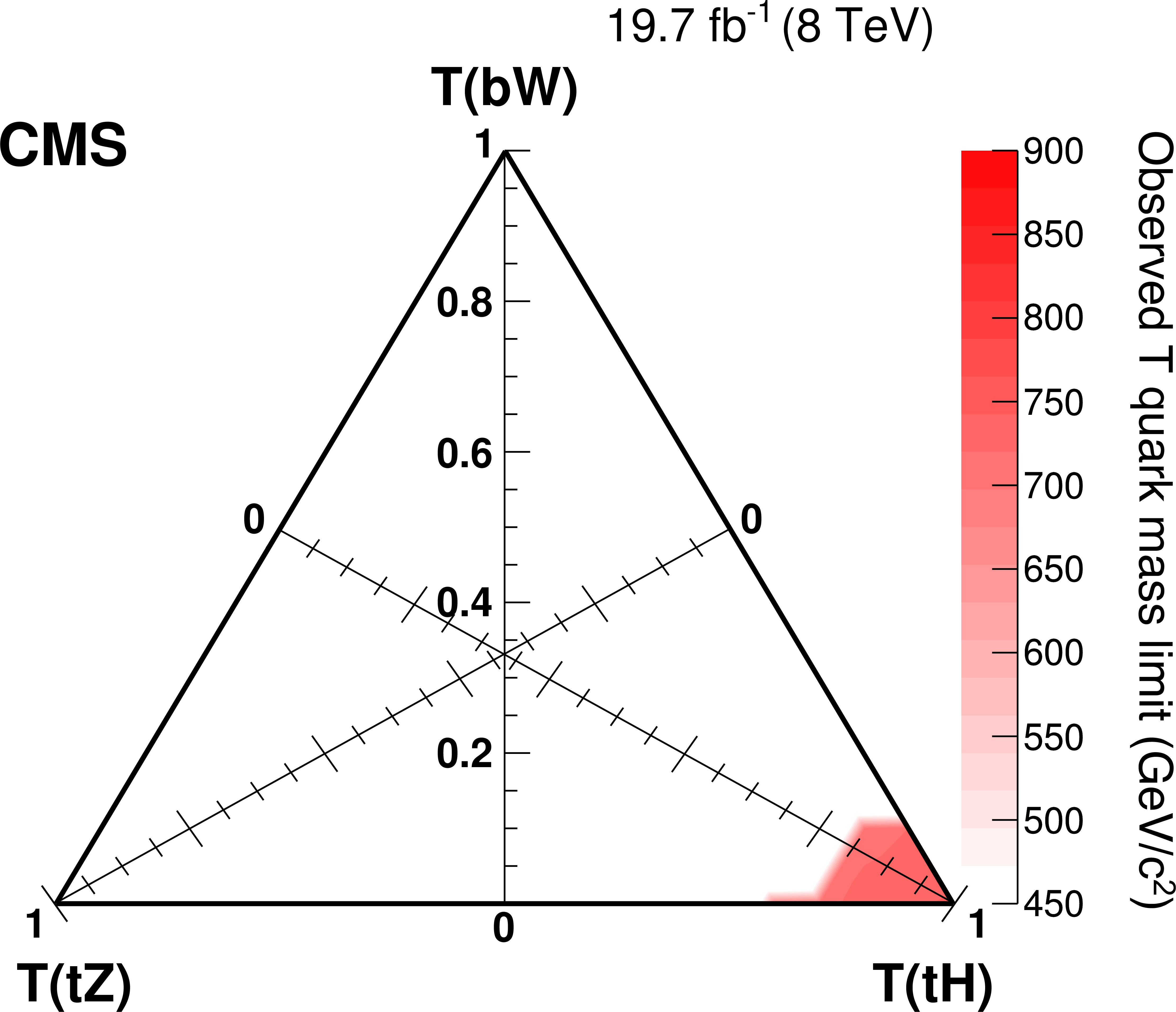
Figure 14-a:
Branching fraction triangle with observed upper limits (a) and expected limits (b) for the T quark mass. Every point in the triangle corresponds to a particular set of branching fraction values subject to the constraint that all three add up to one. The branching fraction for each mode decreases from one at the corner labelled with the specific decay mode to zero at the opposite side of the triangle. |
png pdf |
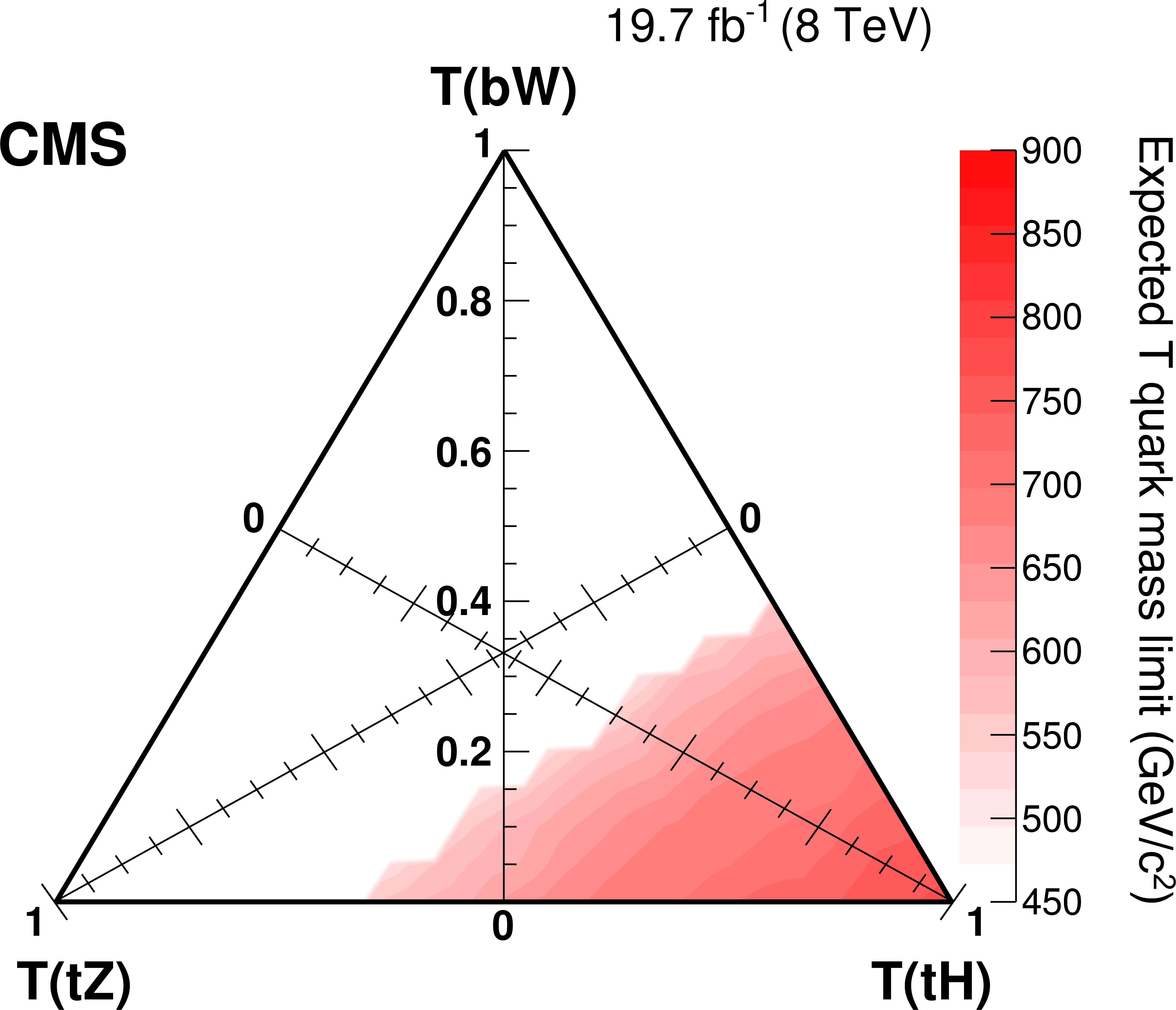
Figure 14-b:
Branching fraction triangle with observed upper limits (a) and expected limits (b) for the T quark mass. Every point in the triangle corresponds to a particular set of branching fraction values subject to the constraint that all three add up to one. The branching fraction for each mode decreases from one at the corner labelled with the specific decay mode to zero at the opposite side of the triangle. |
png pdf |
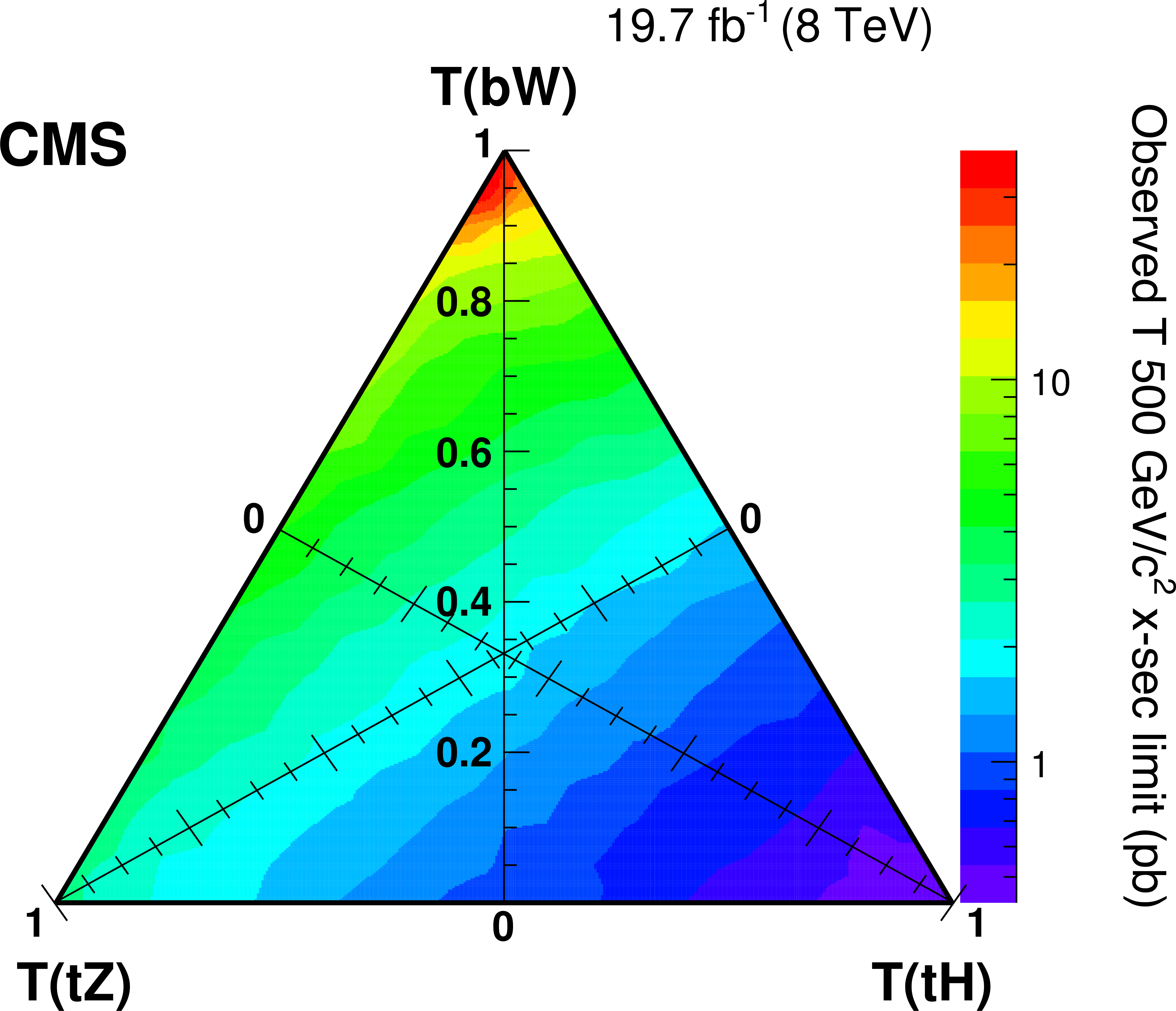
Figure 15-a:
Branching fraction triangle with observed (a, b, c) and expected (d, e, f) limits on the T quark pair production cross section for three different T quark mass hypotheses: 500 (a, d), 700 (b, e), and 1000 GeV/$c^2$ (c, f). Every point in the triangle corresponds to a particular set of branching fraction values subject to the constraint that all three add up to one. The branching fraction for each mode decreases from one at the corner labelled with the specific decay mode to zero at the opposite side of the triangle. |
png pdf |
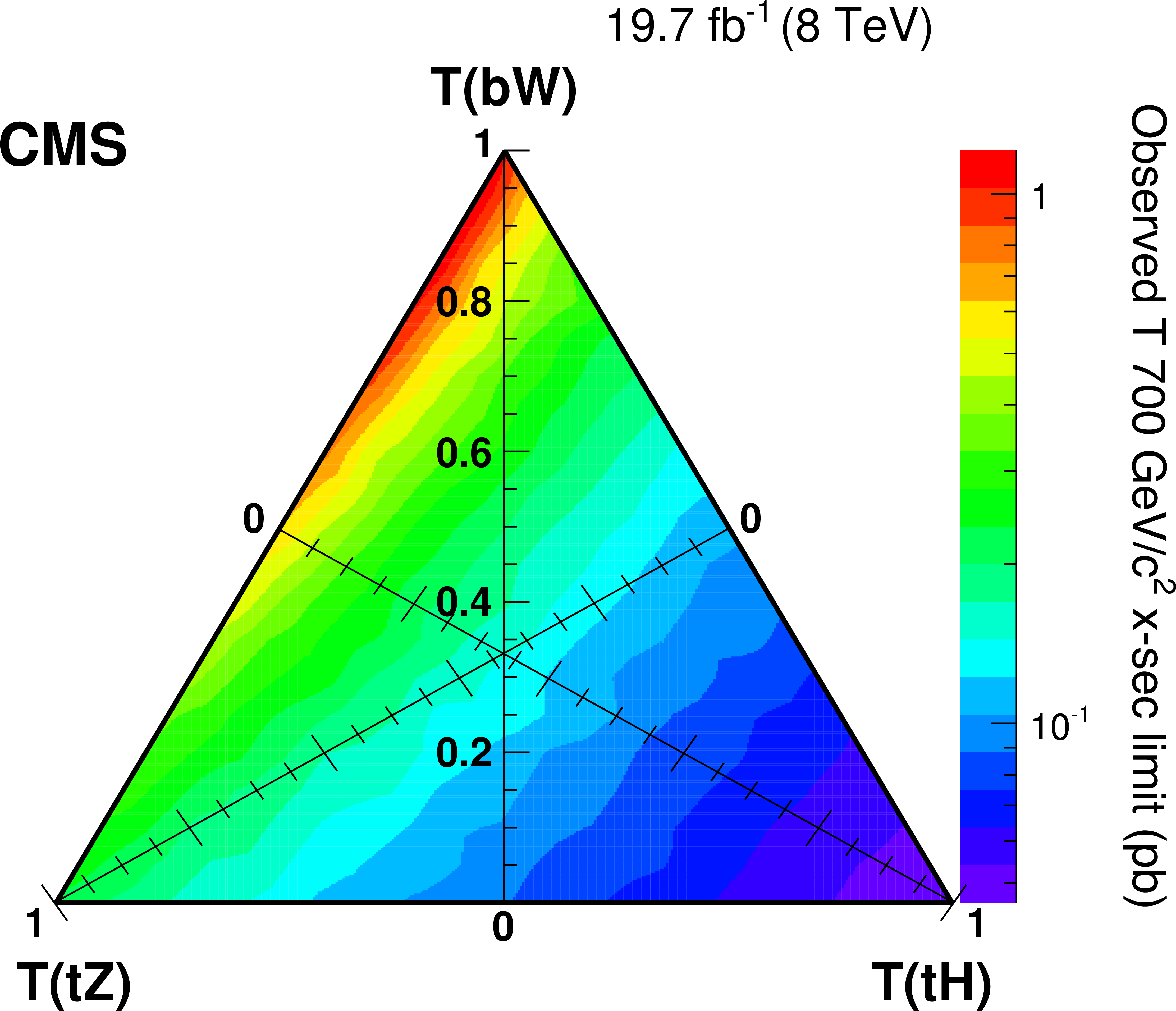
Figure 15-b:
Branching fraction triangle with observed (a, b, c) and expected (d, e, f) limits on the T quark pair production cross section for three different T quark mass hypotheses: 500 (a, d), 700 (b, e), and 1000 GeV/$c^2$ (c, f). Every point in the triangle corresponds to a particular set of branching fraction values subject to the constraint that all three add up to one. The branching fraction for each mode decreases from one at the corner labelled with the specific decay mode to zero at the opposite side of the triangle. |
png pdf |
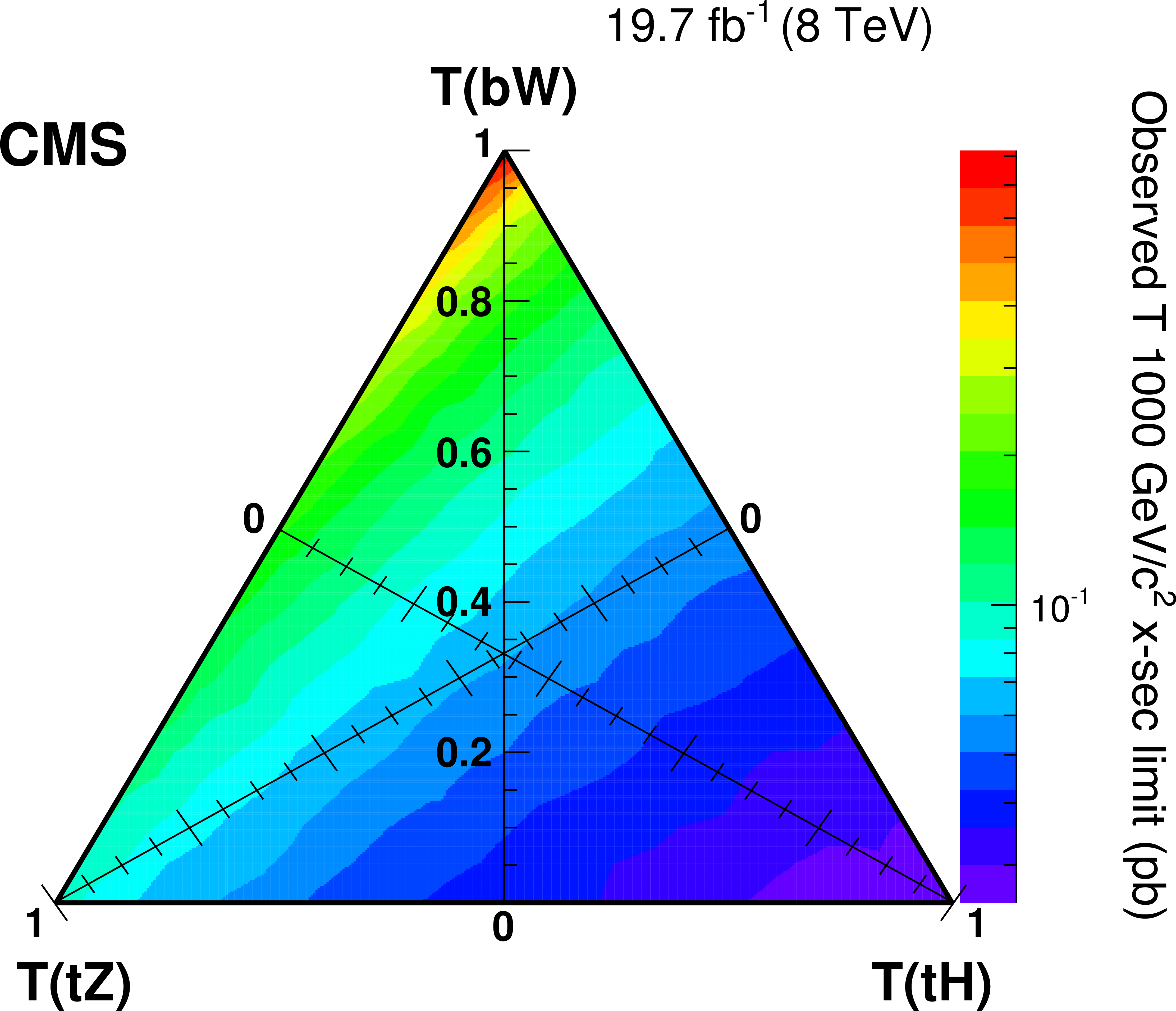
Figure 15-c:
Branching fraction triangle with observed (a, b, c) and expected (d, e, f) limits on the T quark pair production cross section for three different T quark mass hypotheses: 500 (a, d), 700 (b, e), and 1000 GeV/$c^2$ (c, f). Every point in the triangle corresponds to a particular set of branching fraction values subject to the constraint that all three add up to one. The branching fraction for each mode decreases from one at the corner labelled with the specific decay mode to zero at the opposite side of the triangle. |
png pdf |
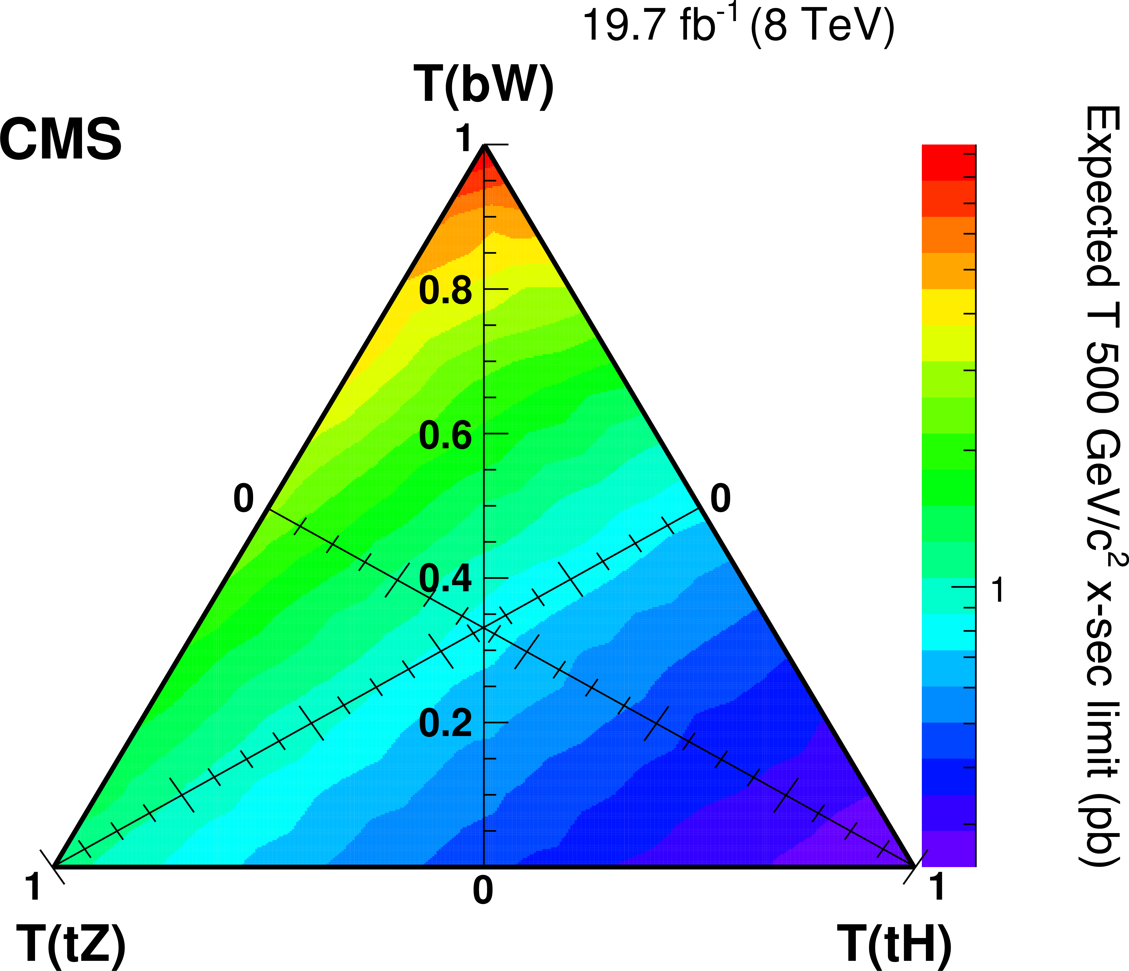
Figure 15-d:
Branching fraction triangle with observed (a, b, c) and expected (d, e, f) limits on the T quark pair production cross section for three different T quark mass hypotheses: 500 (a, d), 700 (b, e), and 1000 GeV/$c^2$ (c, f). Every point in the triangle corresponds to a particular set of branching fraction values subject to the constraint that all three add up to one. The branching fraction for each mode decreases from one at the corner labelled with the specific decay mode to zero at the opposite side of the triangle. |
png pdf |
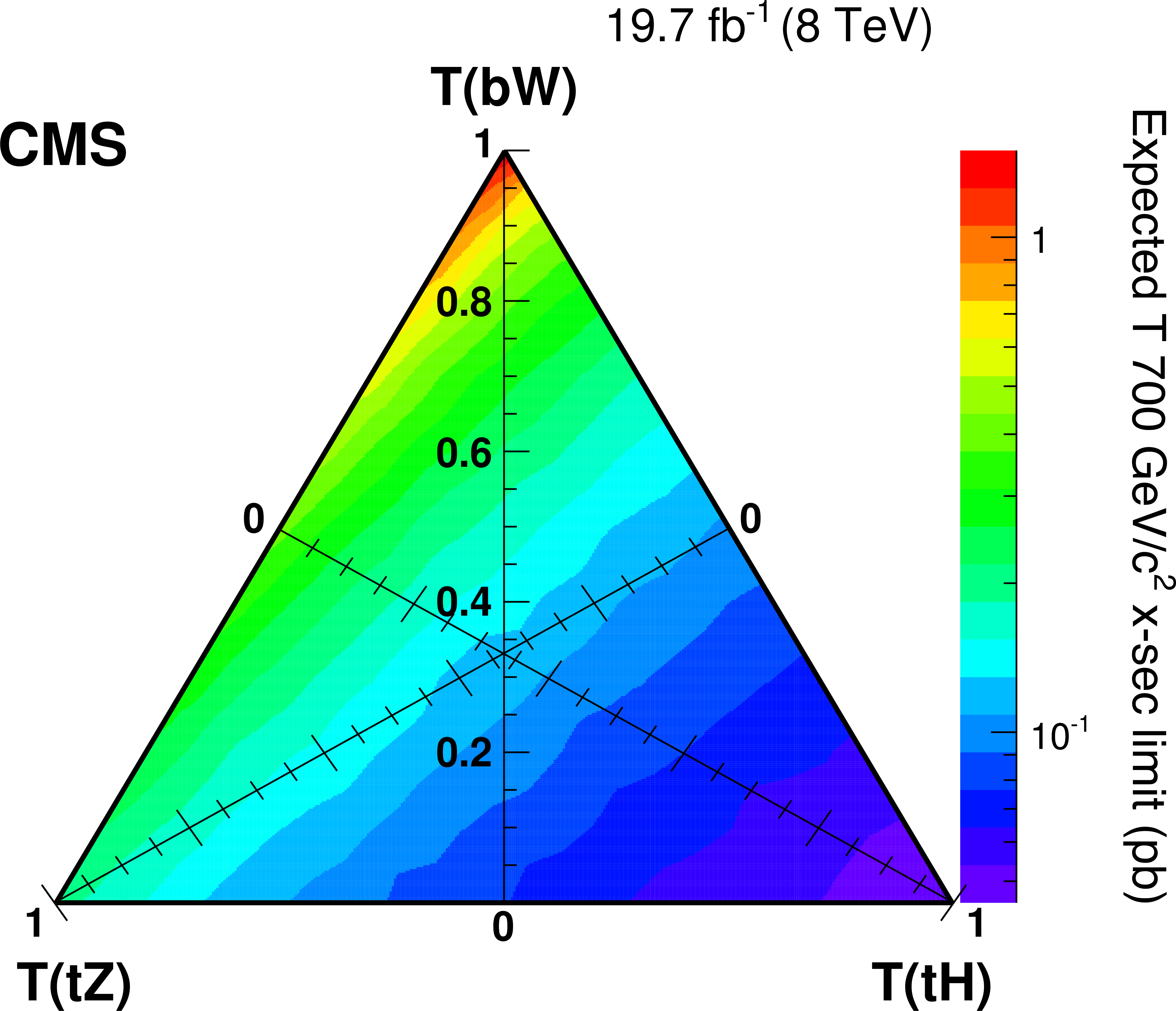
Figure 15-e:
Branching fraction triangle with observed (a, b, c) and expected (d, e, f) limits on the T quark pair production cross section for three different T quark mass hypotheses: 500 (a, d), 700 (b, e), and 1000 GeV/$c^2$ (c, f). Every point in the triangle corresponds to a particular set of branching fraction values subject to the constraint that all three add up to one. The branching fraction for each mode decreases from one at the corner labelled with the specific decay mode to zero at the opposite side of the triangle. |
png pdf |
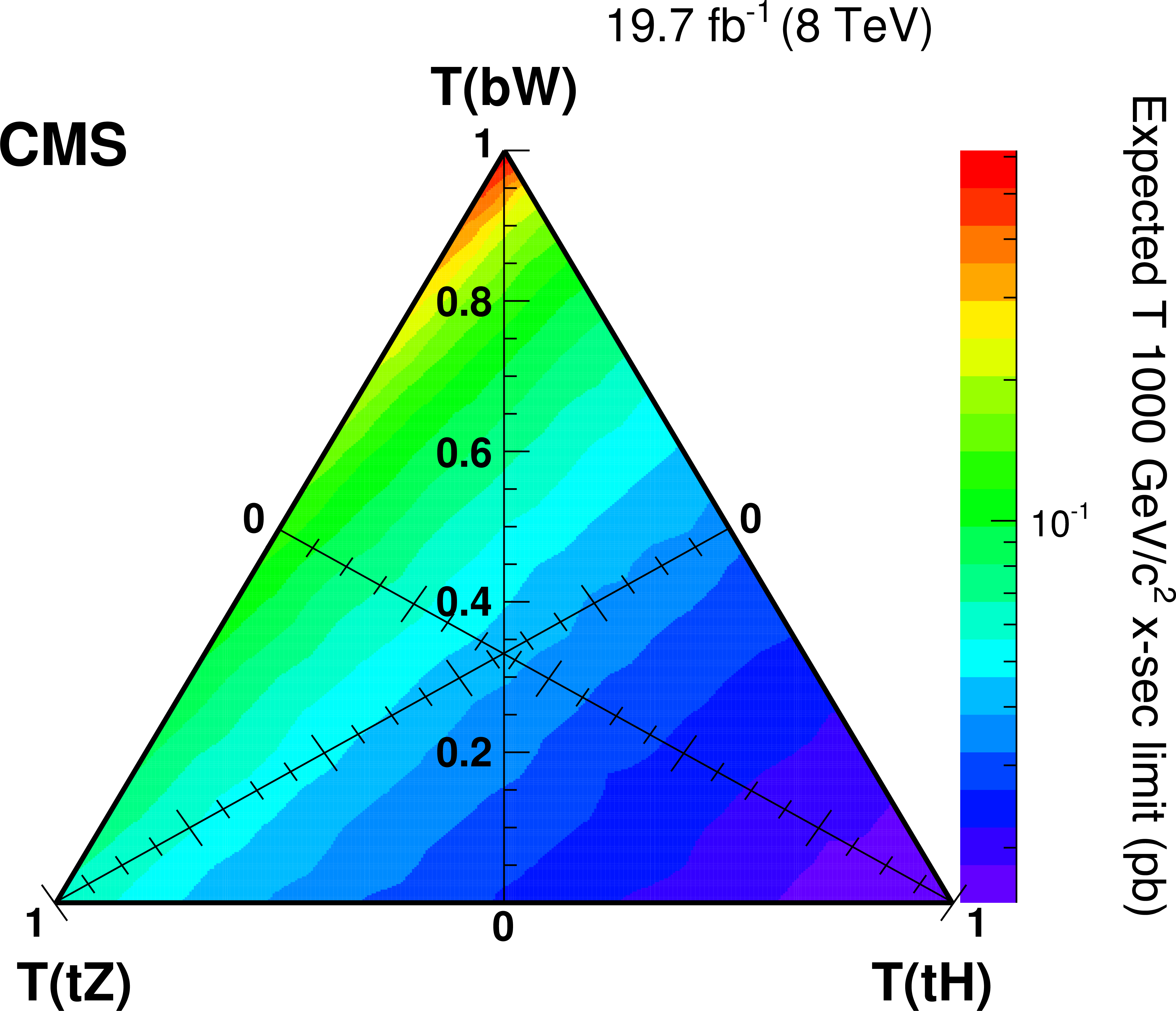
Figure 15-f:
Branching fraction triangle with observed (a, b, c) and expected (d, e, f) limits on the T quark pair production cross section for three different T quark mass hypotheses: 500 (a, d), 700 (b, e), and 1000 GeV/$c^2$ (c, f). Every point in the triangle corresponds to a particular set of branching fraction values subject to the constraint that all three add up to one. The branching fraction for each mode decreases from one at the corner labelled with the specific decay mode to zero at the opposite side of the triangle. |
|
|
Compact Muon Solenoid LHC, CERN |
|

|

|

|

|

|