

Compact Muon Solenoid
LHC, CERN
| CMS-EGM-14-001 ; CERN-PH-EP-2015-006 | ||
| Performance of photon reconstruction and identification with the CMS detector in proton-proton collisions at $\sqrt{s}$ = 8 TeV | ||
| CMS Collaboration | ||
| 10 February 2015 | ||
| J. Instrum 10 (2015) P08010 | ||
| Abstract: A description is provided of the performance of the CMS detector for photon reconstruction and identification in proton-proton collisions at a centre-of-mass energy of 8 TeV at the CERN LHC. Details are given on the reconstruction of photons from energy deposits in the electromagnetic calorimeter (ECAL) and the extraction of photon energy estimates. The reconstruction of electron tracks from photons that convert to electrons in the CMS tracker is also described, as is the optimization of the photon energy reconstruction and its accurate modelling in simulation, in the analysis of the Higgs boson decay into two photons. In the barrel section of the ECAL, an energy resolution of about 1% is achieved for unconverted or late-converting photons from H $\to$ $\gamma \gamma$ decays. Different photon identification methods are discussed and their corresponding selection efficiencies in data are compared with those found in simulated events. The measurement of the photon purity is described for one set of photon identification criteria. | ||
| Links: e-print arXiv:1502.02702 [physics.ins-det] (PDF) ; CDS record ; inSPIRE record ; CADI line (restricted) ; | ||
| Figures | |
png pdf |
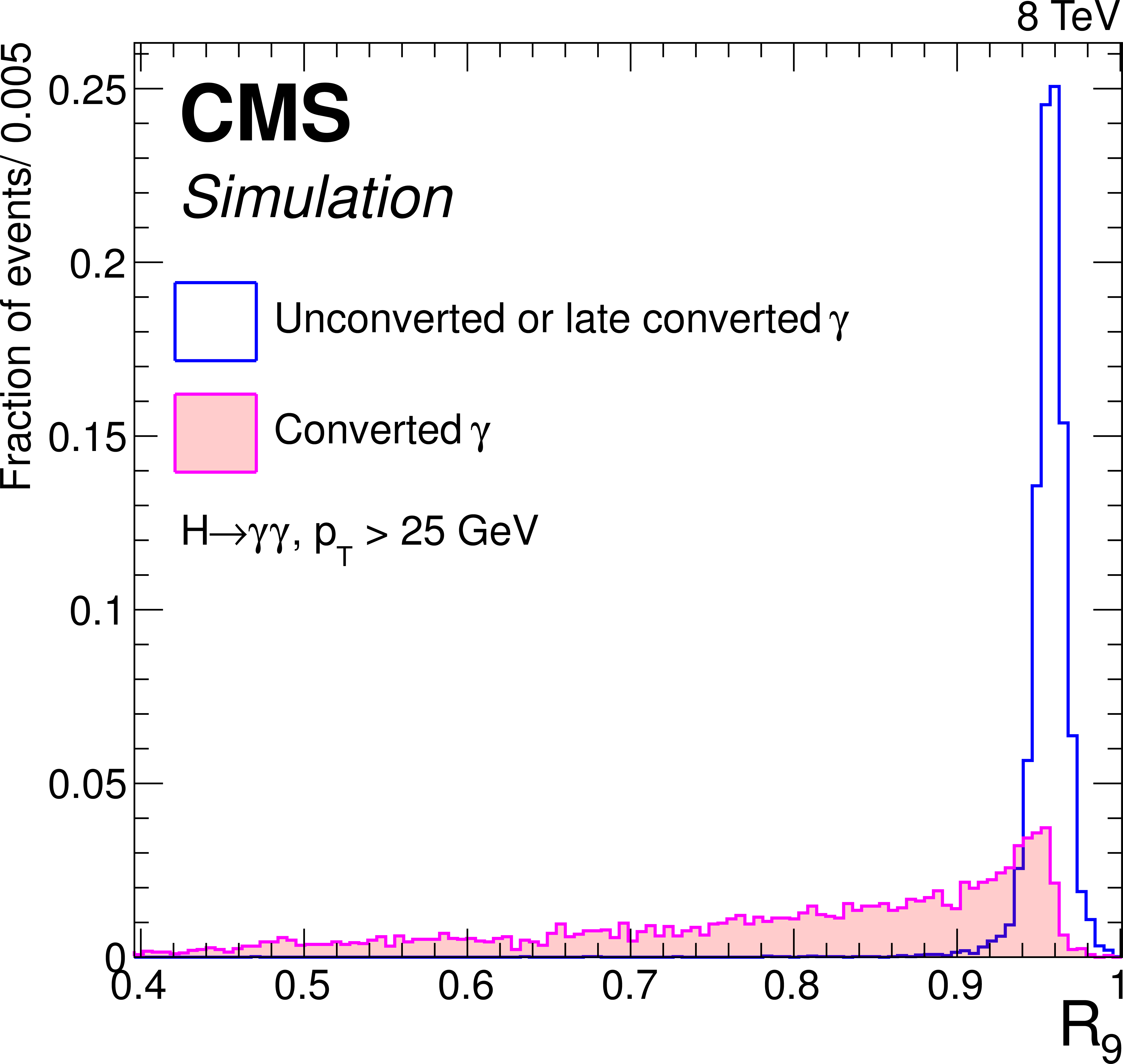
Figure 1:
Distributions of the $ {R_\mathrm {9}}$ variable for photons in the ECAL barrel that convert in the material of the tracker before a radius of 85 cm (solid filled histogram), and those that convert later, or do not convert at all before reaching the ECAL (outlined histogram). |
png pdf |
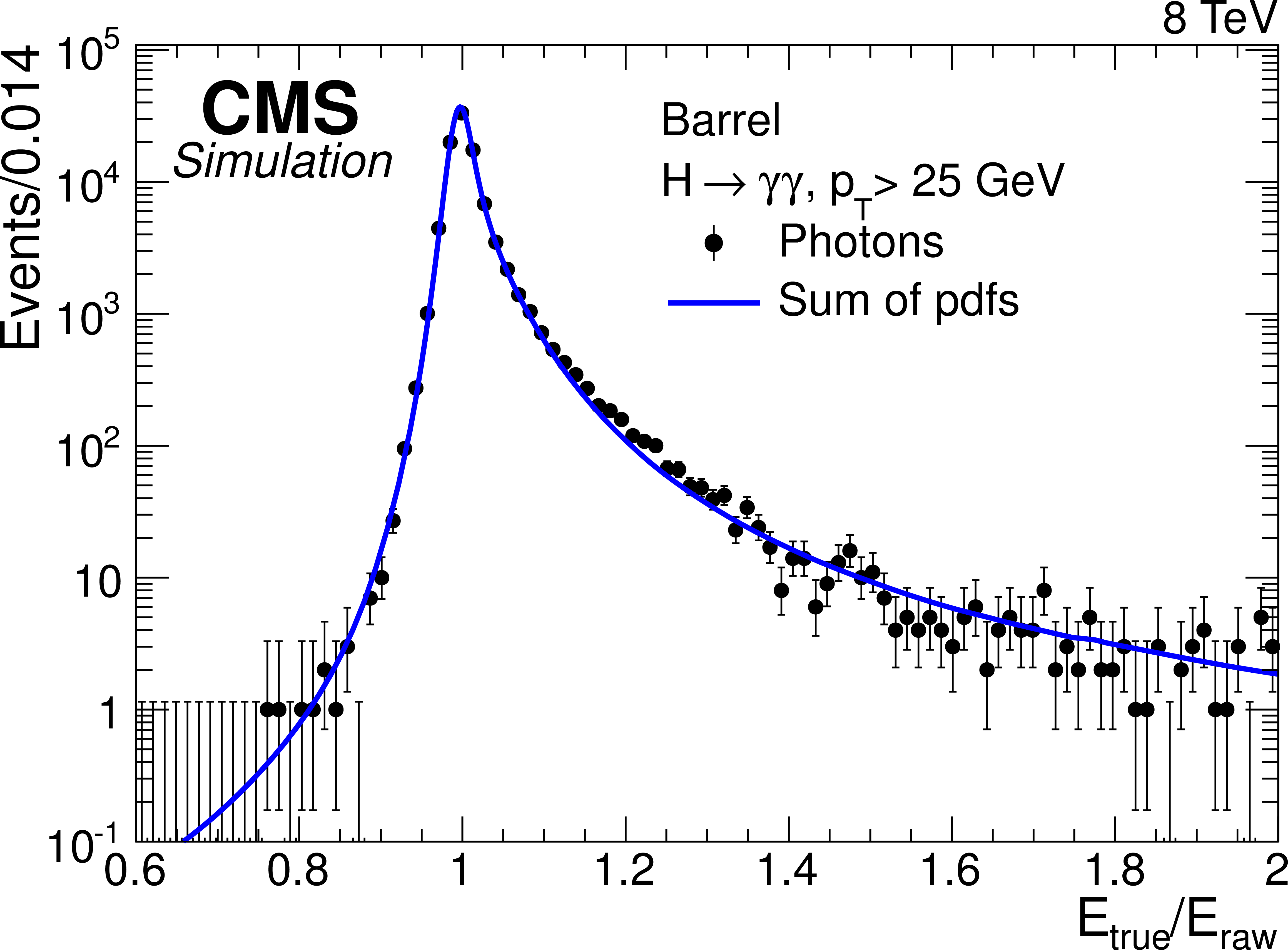
Figure 2-a:
Comparison of the distribution of the inverse response, $E_\text {true}/E_\text {raw}$, in simulated events (points with error bars) with the sum of the pdfs predicted by the regression (curve). The comparison is made using a set of simulated photons independent of the training sample, in the (a) ECAL barrel and (b) endcap. |

png pdf |
Figure 2-b:
Comparison of the distribution of the inverse response, $E_\text {true}/E_\text {raw}$, in simulated events (points with error bars) with the sum of the pdfs predicted by the regression (curve). The comparison is made using a set of simulated photons independent of the training sample, in the (a) ECAL barrel and (b) endcap. |
png pdf |
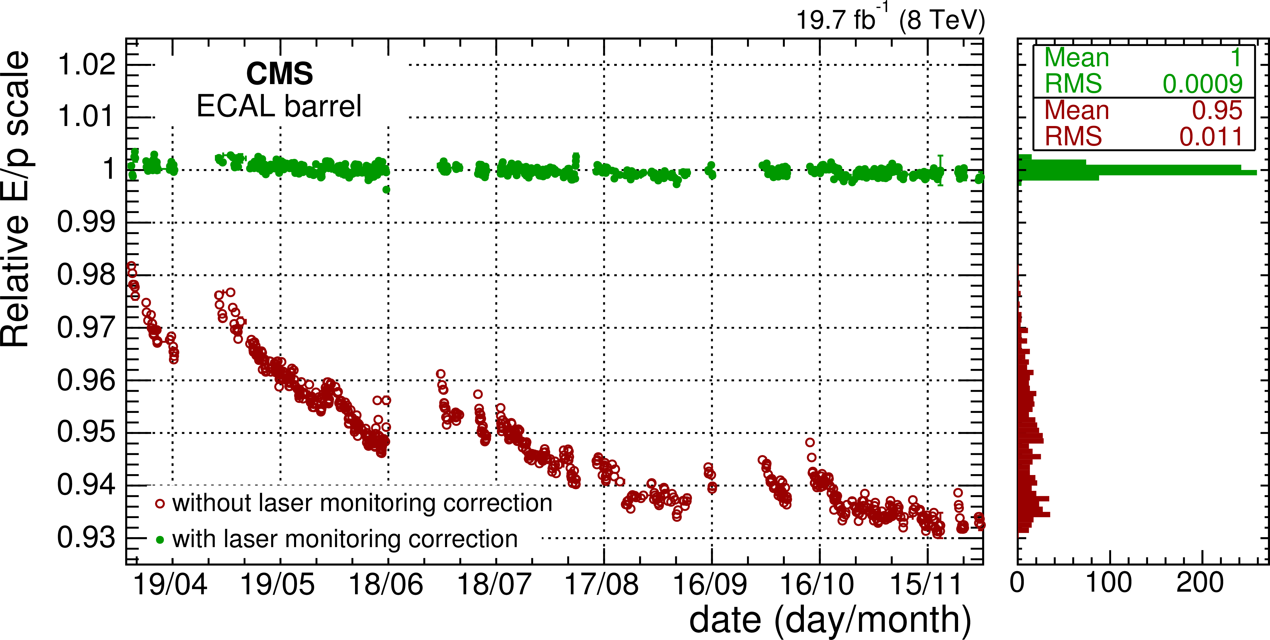
Figure 3-a:
Ratio of the energy measured by the ECAL over the momentum measured by the tracker, $E/p$, for electrons selected from $ { {\mathrm {W}}\to {\mathrm {e}} {\nu }} $ decays, as a function of the date at which they were recorded. The ratio is shown both before (red points), and after (green points), the application of transparency corrections obtained from the laser monitoring system, and for both the barrel (upper plot) and the endcaps (lower plot). Histograms of the values of the measured points, together with their mean and RMS values are shown beside the main plots. |
png pdf |
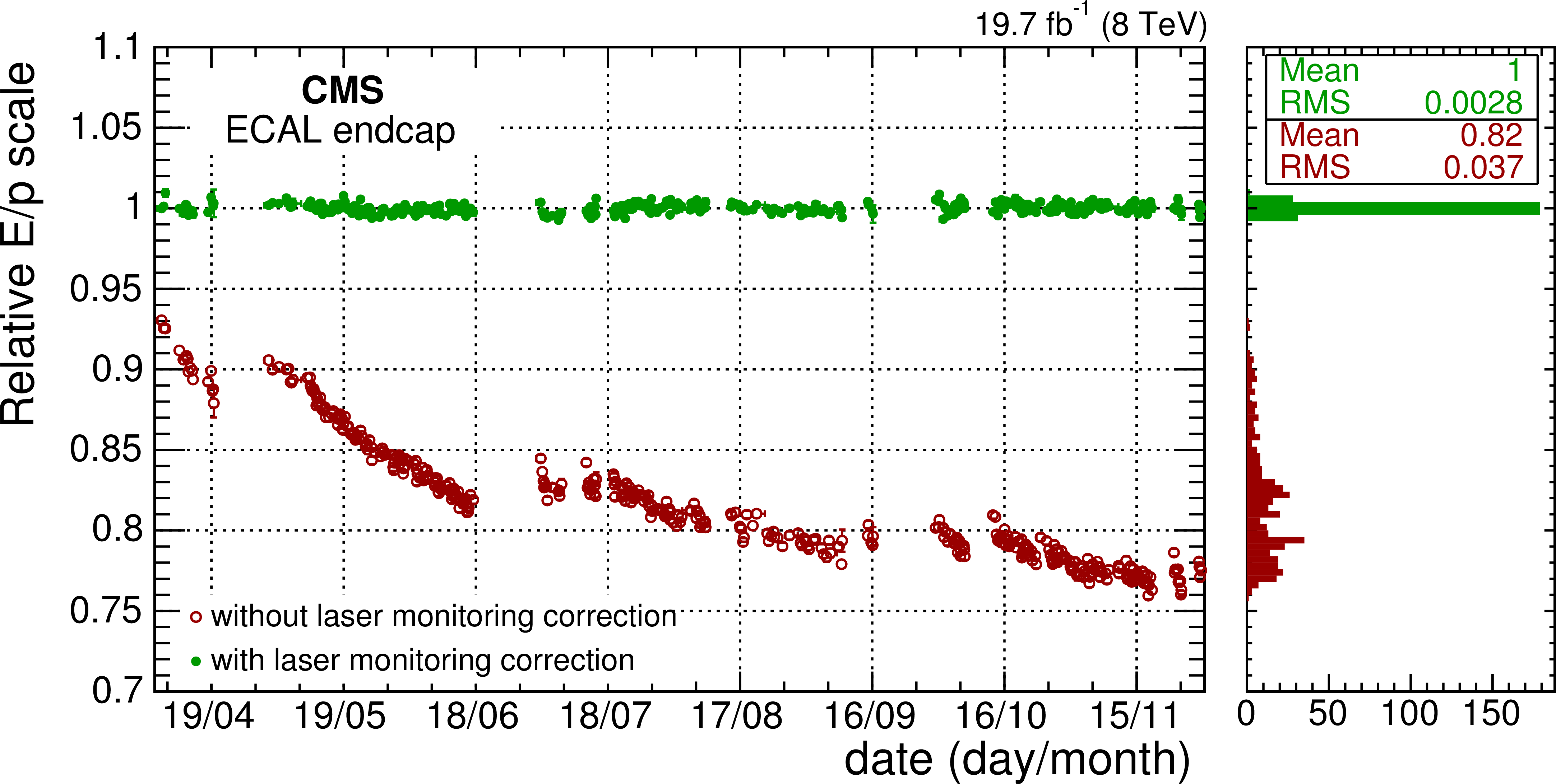
Figure 3-b:
Ratio of the energy measured by the ECAL over the momentum measured by the tracker, $E/p$, for electrons selected from $ { {\mathrm {W}}\to {\mathrm {e}} {\nu }} $ decays, as a function of the date at which they were recorded. The ratio is shown both before (red points), and after (green points), the application of transparency corrections obtained from the laser monitoring system, and for both the barrel (upper plot) and the endcaps (lower plot). Histograms of the values of the measured points, together with their mean and RMS values are shown beside the main plots. |
png pdf |
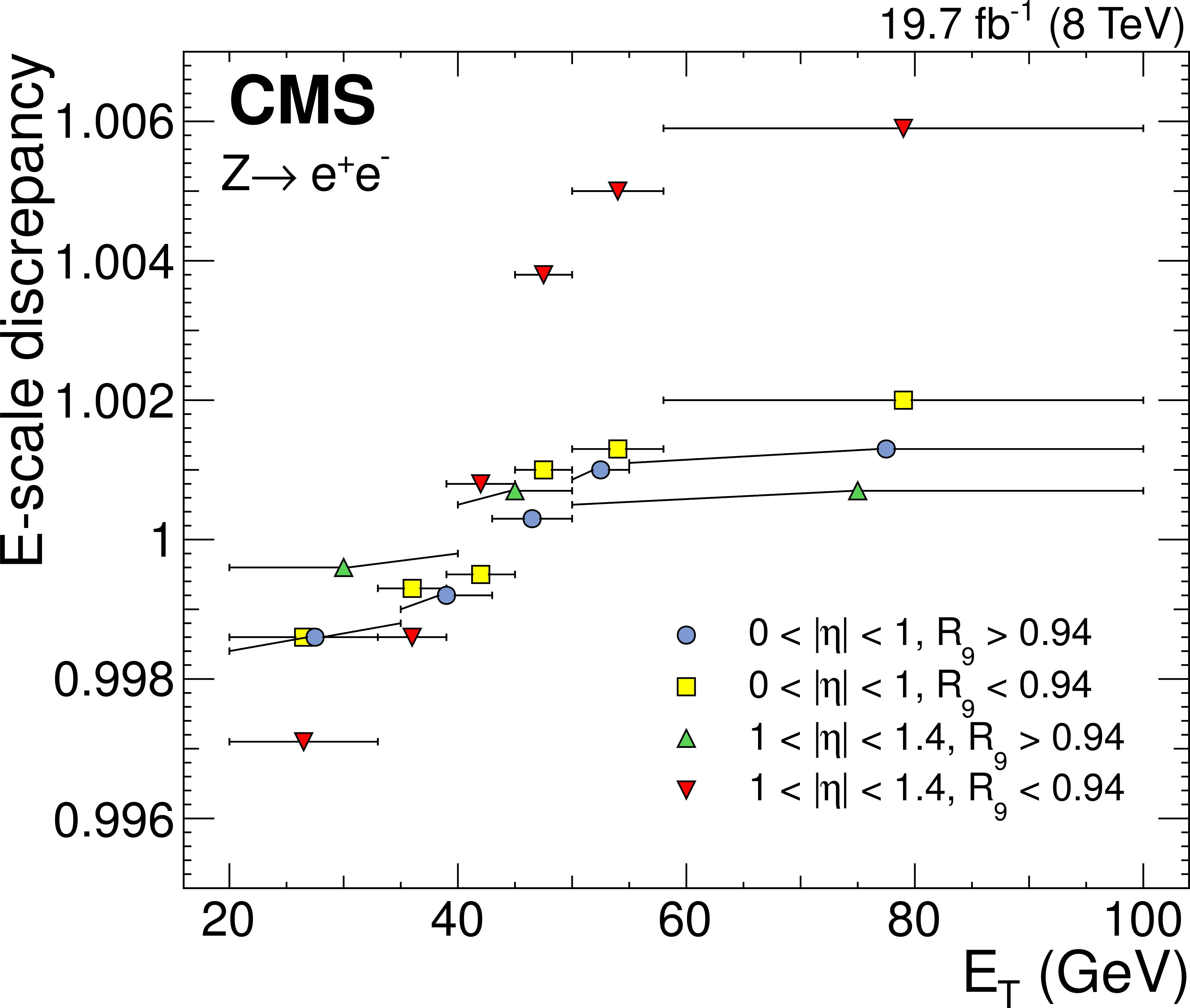
Figure 4:
Residual discrepancies in the photon energy scale obtained for the barrel in the final step of the fine-tuning procedure, as a function of $ {E_{\mathrm {T}}} $, for different $\eta $ and $ {R_\mathrm {9}}$ categories. The statistical uncertainties in these values are negligible. The horizontal error bars indicate the ranges of the $ {E_{\mathrm {T}}} $ bins. The reciprocals of these values are applied as corrections to the energy scale. Some of the error bars have been deflected vertically to avoid overlap with others. |

png pdf |
Figure 5:
Reconstructed invariant mass distribution of electron pairs in $ { {\mathrm {Z}}\to {\mathrm {e}^+} {\mathrm {e}^-}} $ events in data (points) and in simulation (histogram). The electrons are reconstructed as photons and the full set of photon corrections and smearings are applied. The comparison is shown for (left) events with both showers in the barrel and (right) the remaining events. For each bin, the ratio of the number of events in data to the number of simulated events is shown in the panels beneath the main plot. The band shows the systematic uncertainty in the ratio originating in the systematic uncertainty in the simulated energy resolution, and in the data energy scale. |
png pdf |
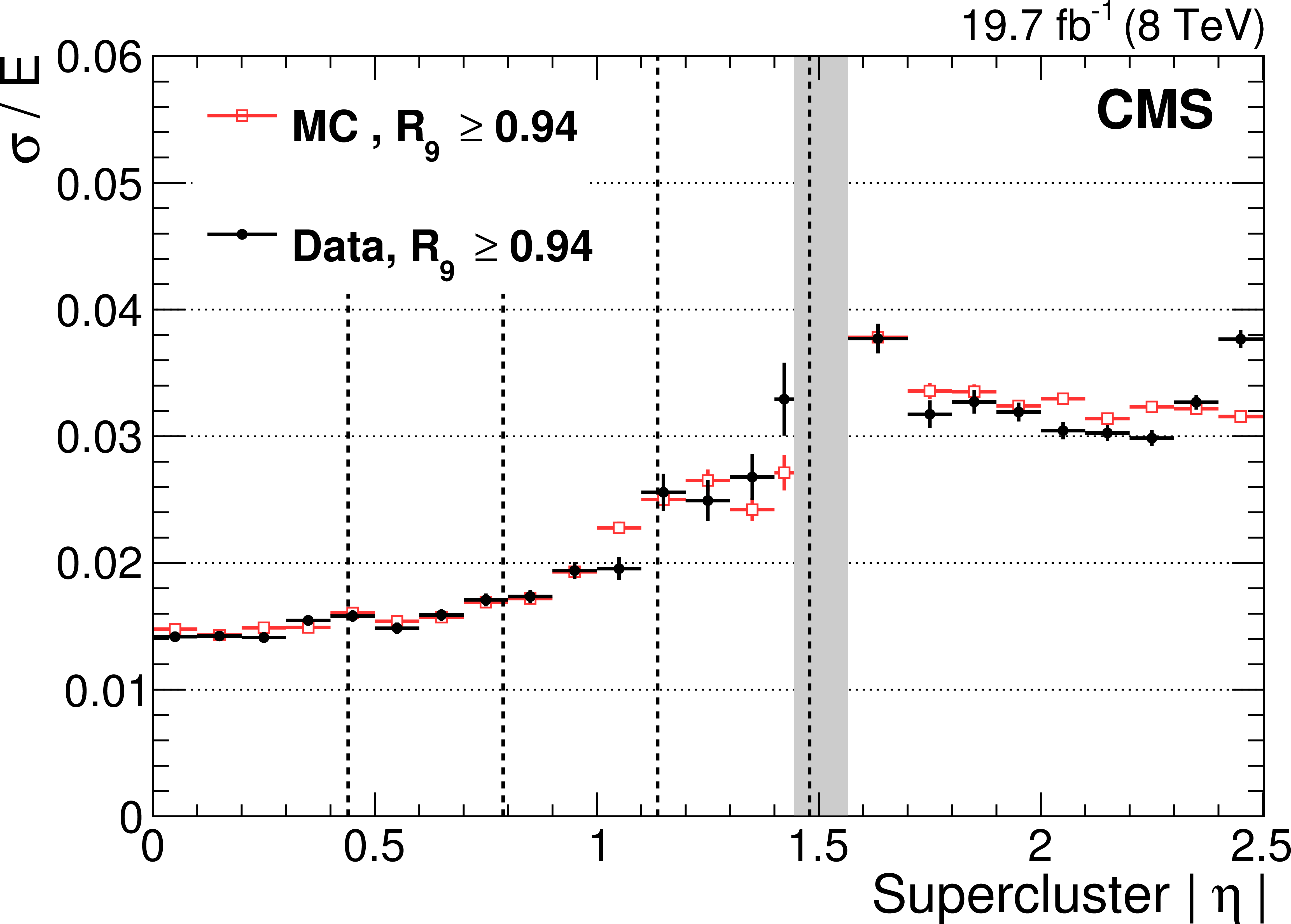
Figure 6-a:
Relative photon energy resolution measured in small bins of absolute supercluster pseudorapidity in $ { {\mathrm {Z}}\to {\mathrm {e}^+} {\mathrm {e}^-}} $ events, for data (solid black circles) and simulated events (open squares), where the electrons are reconstructed as photons. The resolution is shown for (upper plot) showers with $ {R_\mathrm {9}}\ge 0.94$ and (lower plot) $ {R_\mathrm {9}}<0.94$. The vertical dashed lines mark the module boundaries in the barrel, and the vertical grey band indicates the range of $ {| \eta | }$, around the barrel/endcap transition, removed from the fiducial region. |
png pdf |
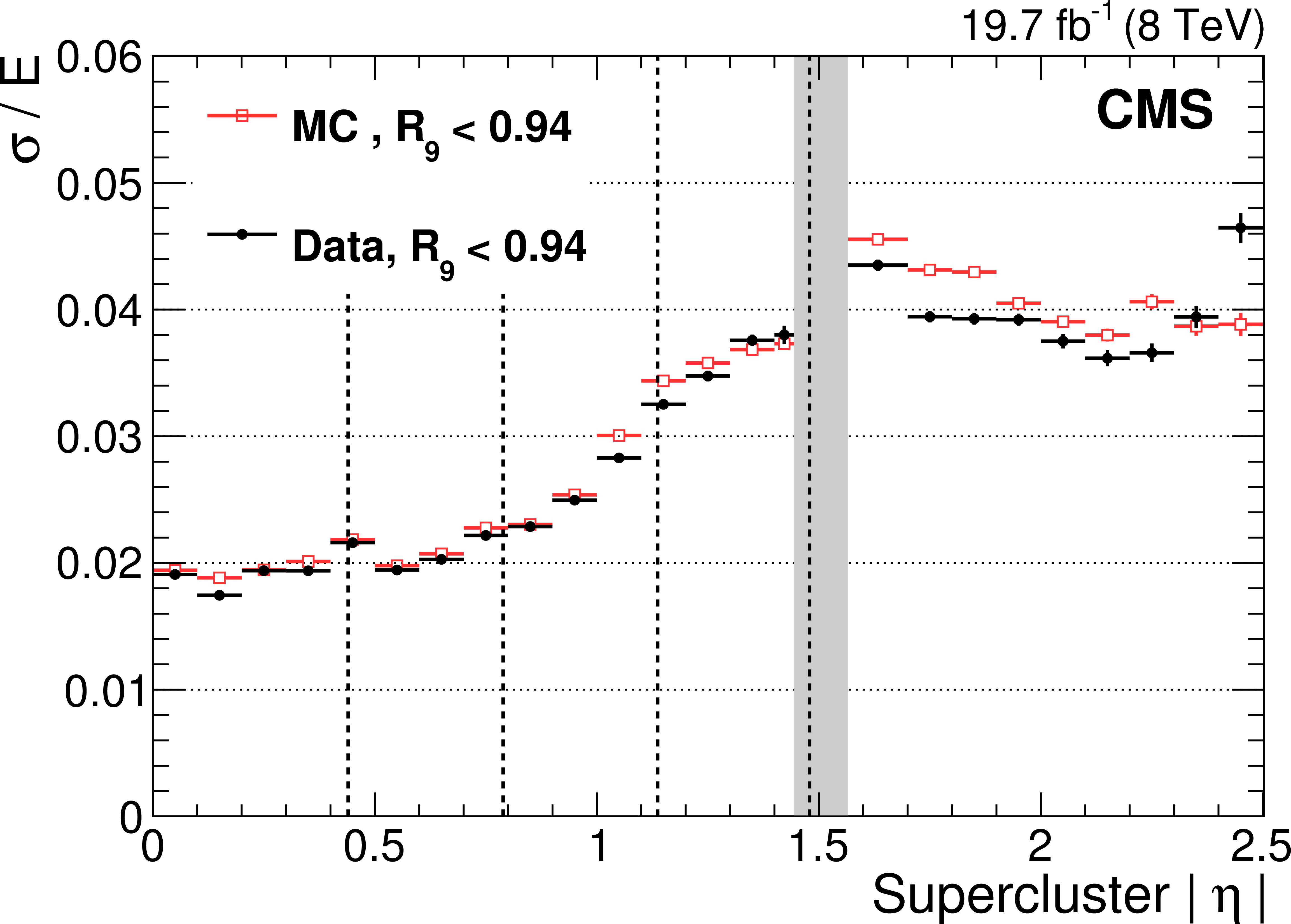
Figure 6-b:
Relative photon energy resolution measured in small bins of absolute supercluster pseudorapidity in $ { {\mathrm {Z}}\to {\mathrm {e}^+} {\mathrm {e}^-}} $ events, for data (solid black circles) and simulated events (open squares), where the electrons are reconstructed as photons. The resolution is shown for (upper plot) showers with $ {R_\mathrm {9}}\ge 0.94$ and (lower plot) $ {R_\mathrm {9}}<0.94$. The vertical dashed lines mark the module boundaries in the barrel, and the vertical grey band indicates the range of $ {| \eta | }$, around the barrel/endcap transition, removed from the fiducial region. |
png pdf |
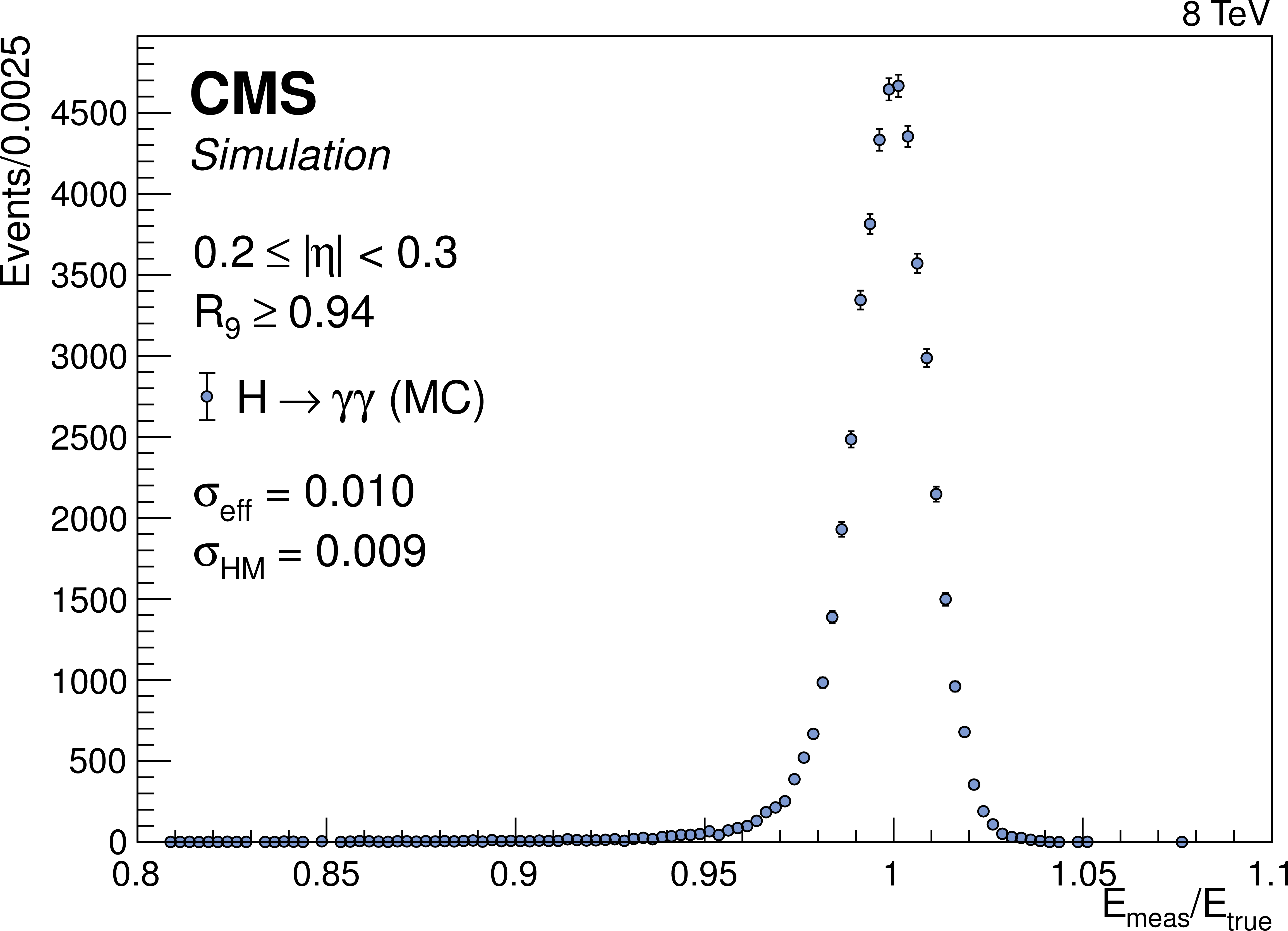
Figure 7-a:
Distribution of measured over true energy, $E_\text {meas}/E_\text {true}$, for photons in simulated $ { {\mathrm {H}} \to {\gamma } {\gamma }} $ events, in a narrow $\eta $ range in the barrel, $0.2< {| \eta | }<0.3$, (left) for photons with $ {R_\mathrm {9}}\geq 0.94$, and (right) $ {R_\mathrm {9}}<0.94$. |
png pdf |
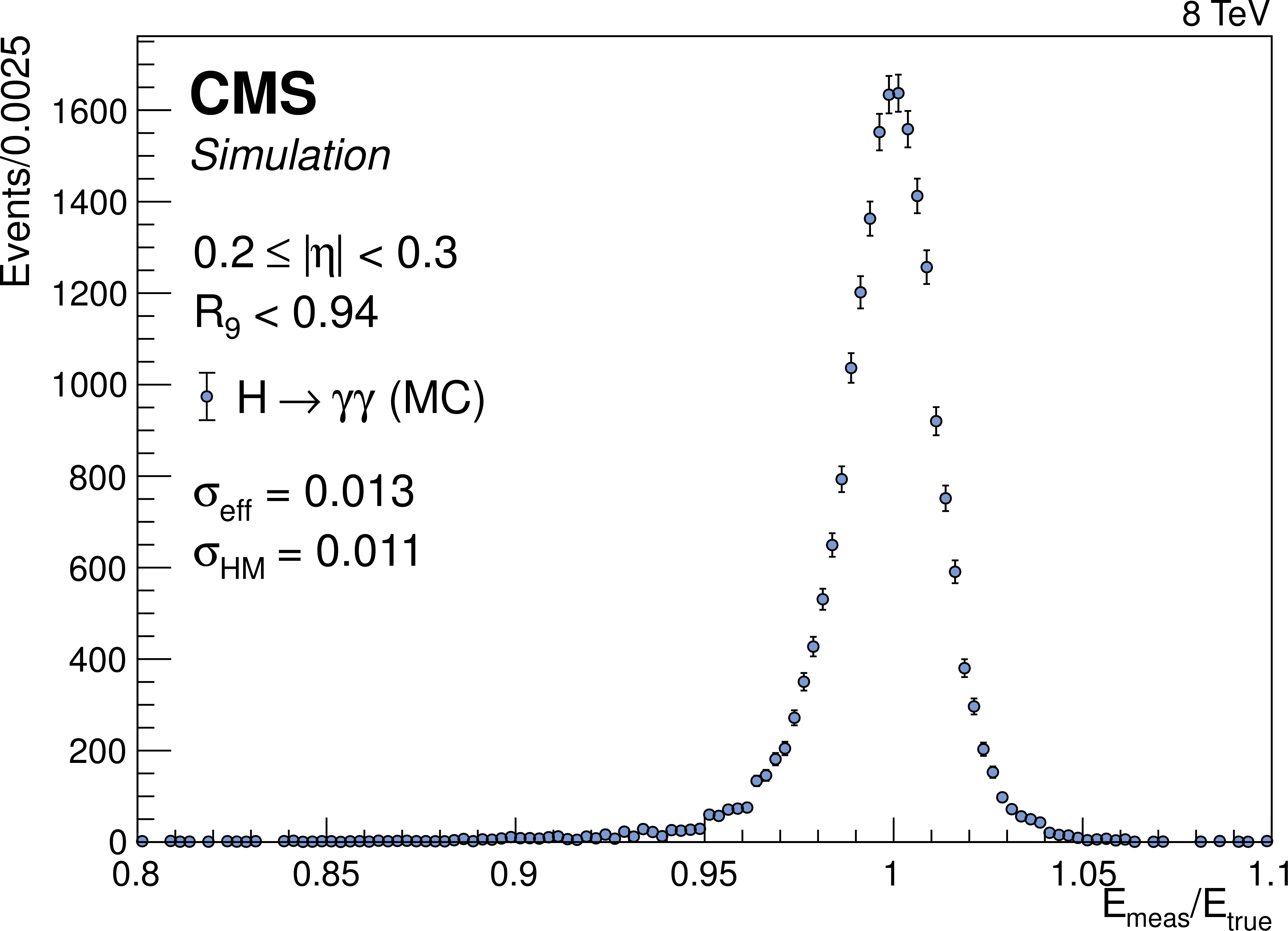
Figure 7-b:
Distribution of measured over true energy, $E_\text {meas}/E_\text {true}$, for photons in simulated $ { {\mathrm {H}} \to {\gamma } {\gamma }} $ events, in a narrow $\eta $ range in the barrel, $0.2< {| \eta | }<0.3$, (left) for photons with $ {R_\mathrm {9}}\geq 0.94$, and (right) $ {R_\mathrm {9}}<0.94$. |
png pdf |
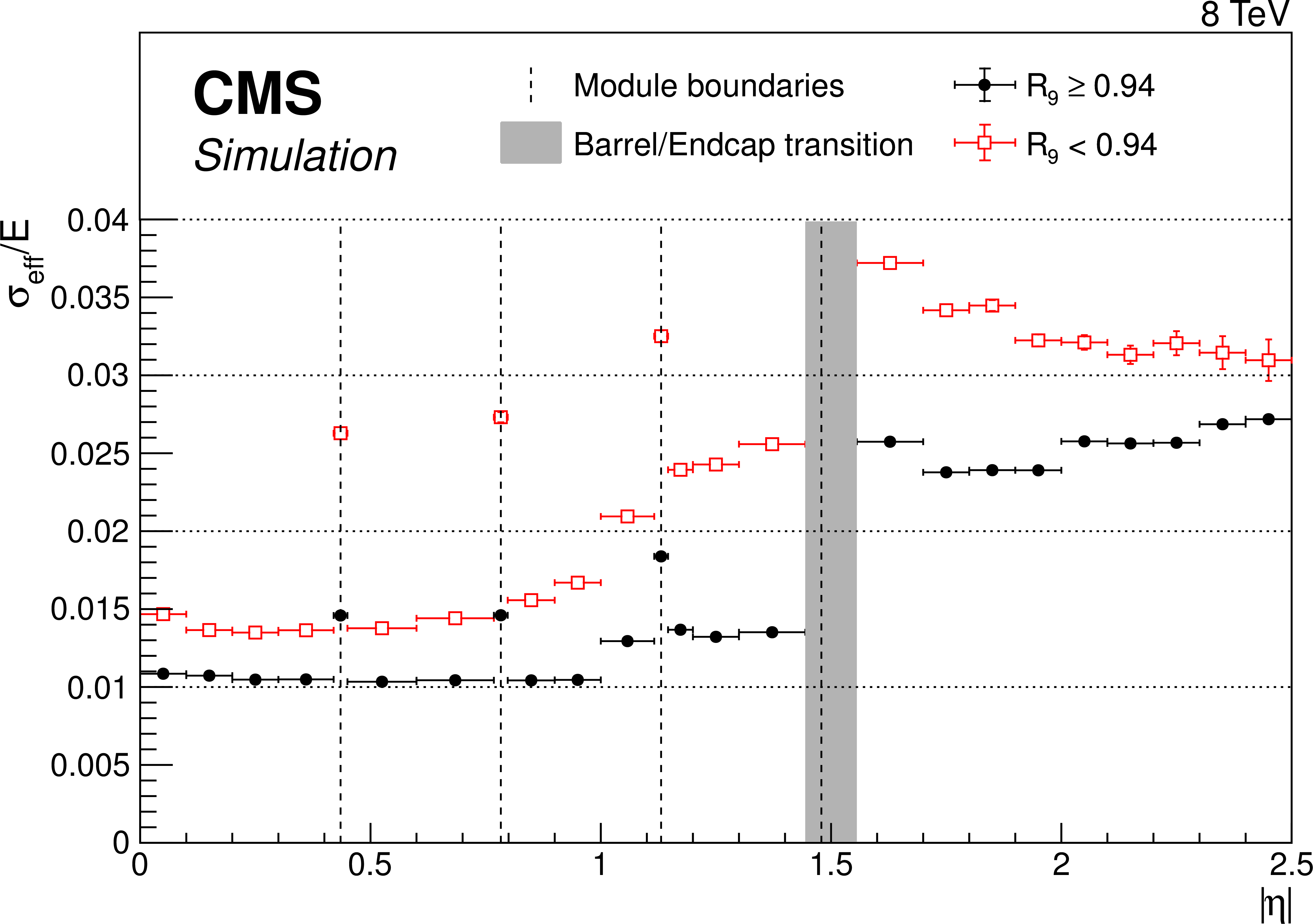
Figure 8:
Relative energy resolution, $\sigma _\text {eff}/E$, as a function of $ {| \eta | }$, in simulated $ { {\mathrm {H}} \to {\gamma } {\gamma }} $ events, for photons with $ {R_\mathrm {9}}\geq 0.94$ (solid circles) and photons with $ {R_\mathrm {9}}<0.94$ (open squares). The vertical dashed lines mark the module boundaries in the barrel, and the vertical grey band indicates the range of $ {| \eta | }$, around the barrel/endcap transition, removed from the fiducial region. |
png pdf |
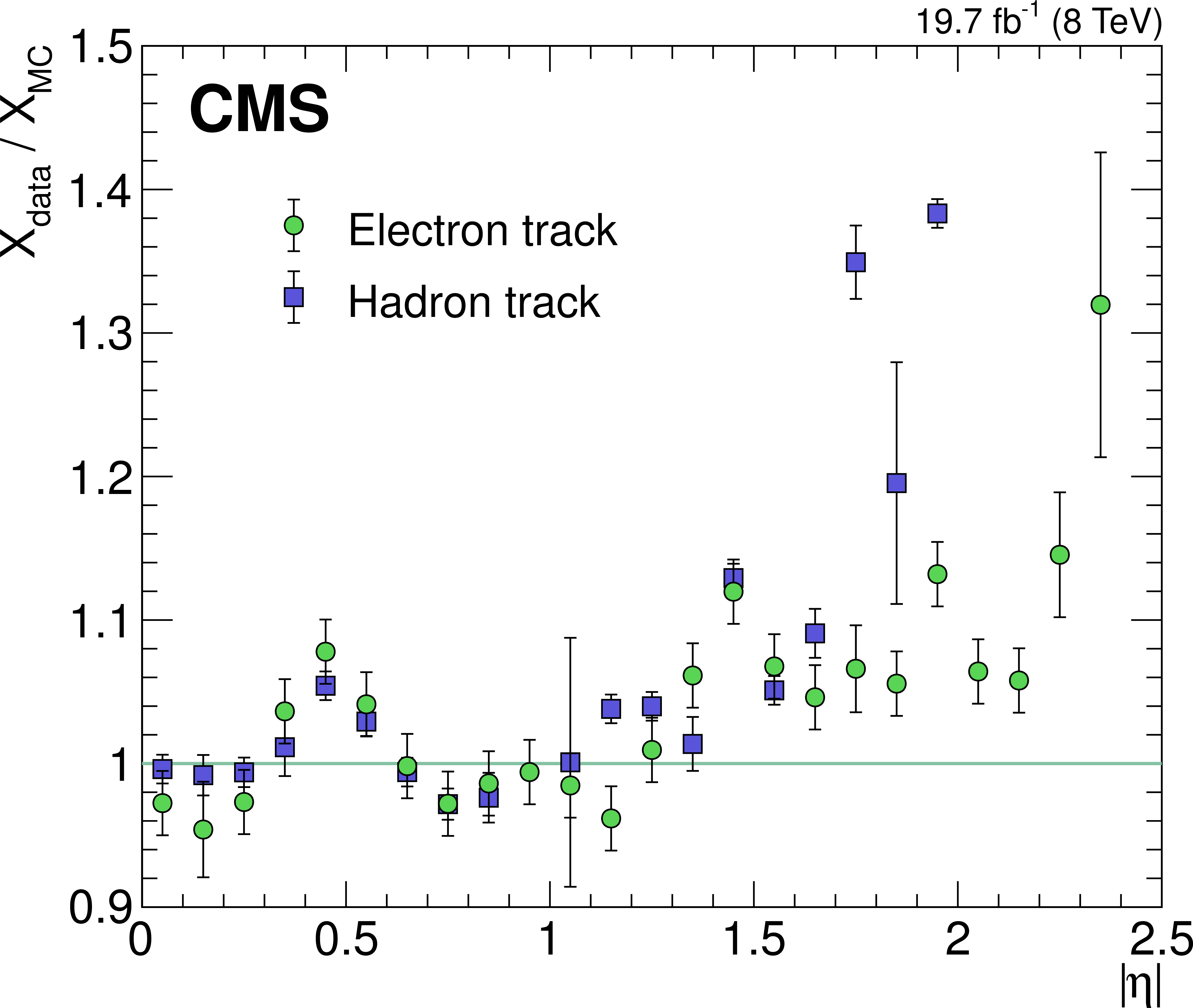
Figure 9:
Tracker material thickness (in terms of radiation lengths) inferred in the data, $X_\text {data}$, relative to that inferred in simulated events, $X_\mathrm {MC}$, as a function of $ {| \eta | }$, using electrons in $ { {\mathrm {Z}}\to {\mathrm {e}^+} {\mathrm {e}^-}} $ events (circles), and low-momentum charged hadrons (squares). |

png pdf |
Figure 10:
Residual discrepancy of the energy response in data relative to that in simulated events as a function of transverse energy (for the $E/p$ analysis, squares) and of $ {H_{\mathrm {T}}} /2$ (for the dielectron mass analysis, circles) in four $\eta $ and $ {R_\mathrm {9}}$ categories. The dielectron analysis is restricted to events where both the electron showers fall in the same $\eta , {R_\mathrm {9}}$ category. The uncertainties in the fit parameters of a linear response model are shown by bands---further details are given in the text. |
png pdf |
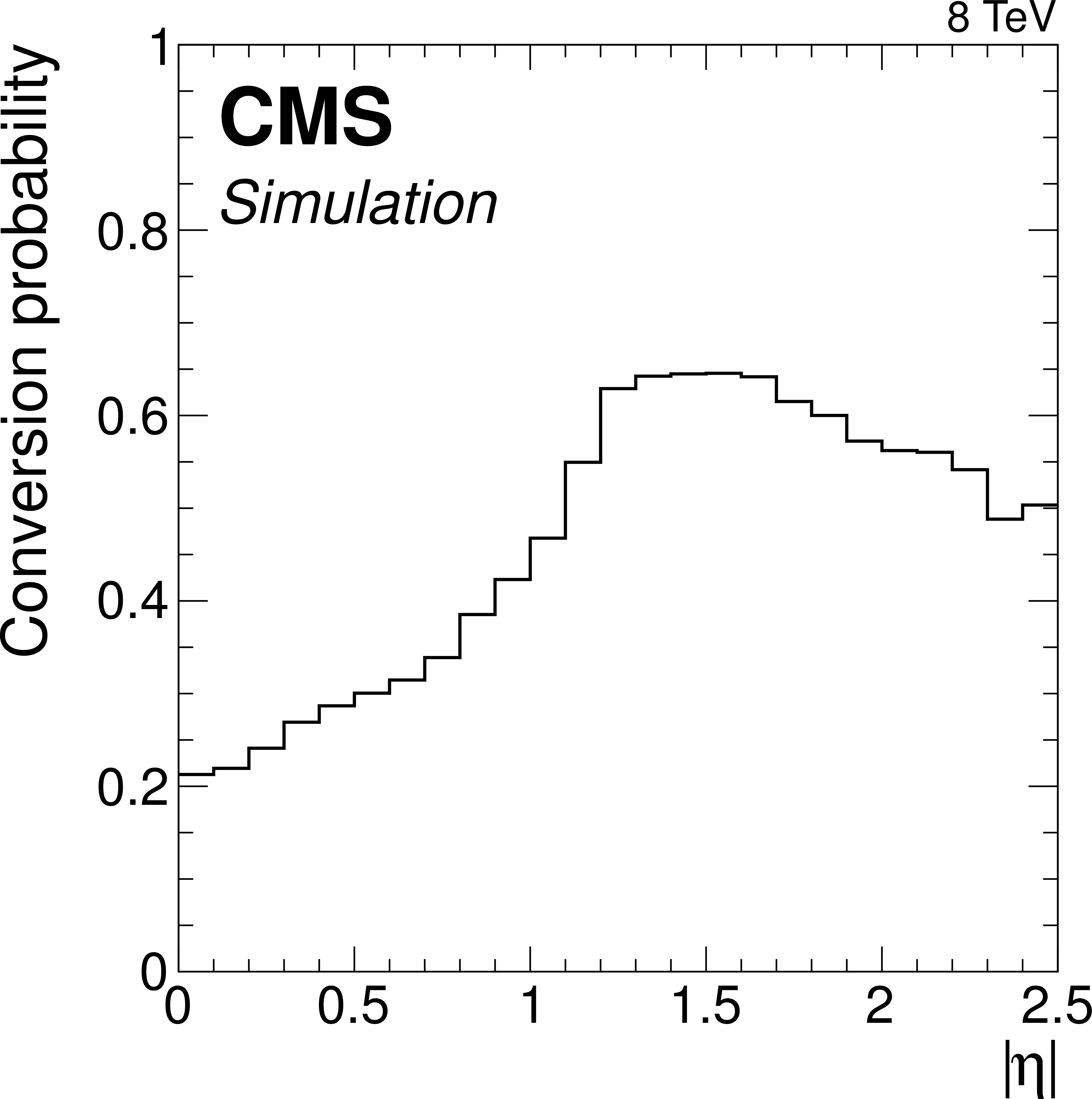
Figure 11:
Fraction of photons converting before the last three layers of the tracker as function of absolute pseudorapidity as measured in a simulated sample of $ { {\mathrm {H}} \to {\gamma } {\gamma }} $ events. The conversion location is obtained from the simulation program. |

png pdf |
Figure 12:
Invariant mass for $ { {\mathrm {Z}}\to {{\mu ^+}} {{\mu ^-}} {\gamma }} $ events in which the photon is associated to a conversion track pair in data (points with error bars) and simulation (filled histogram). |
png pdf |
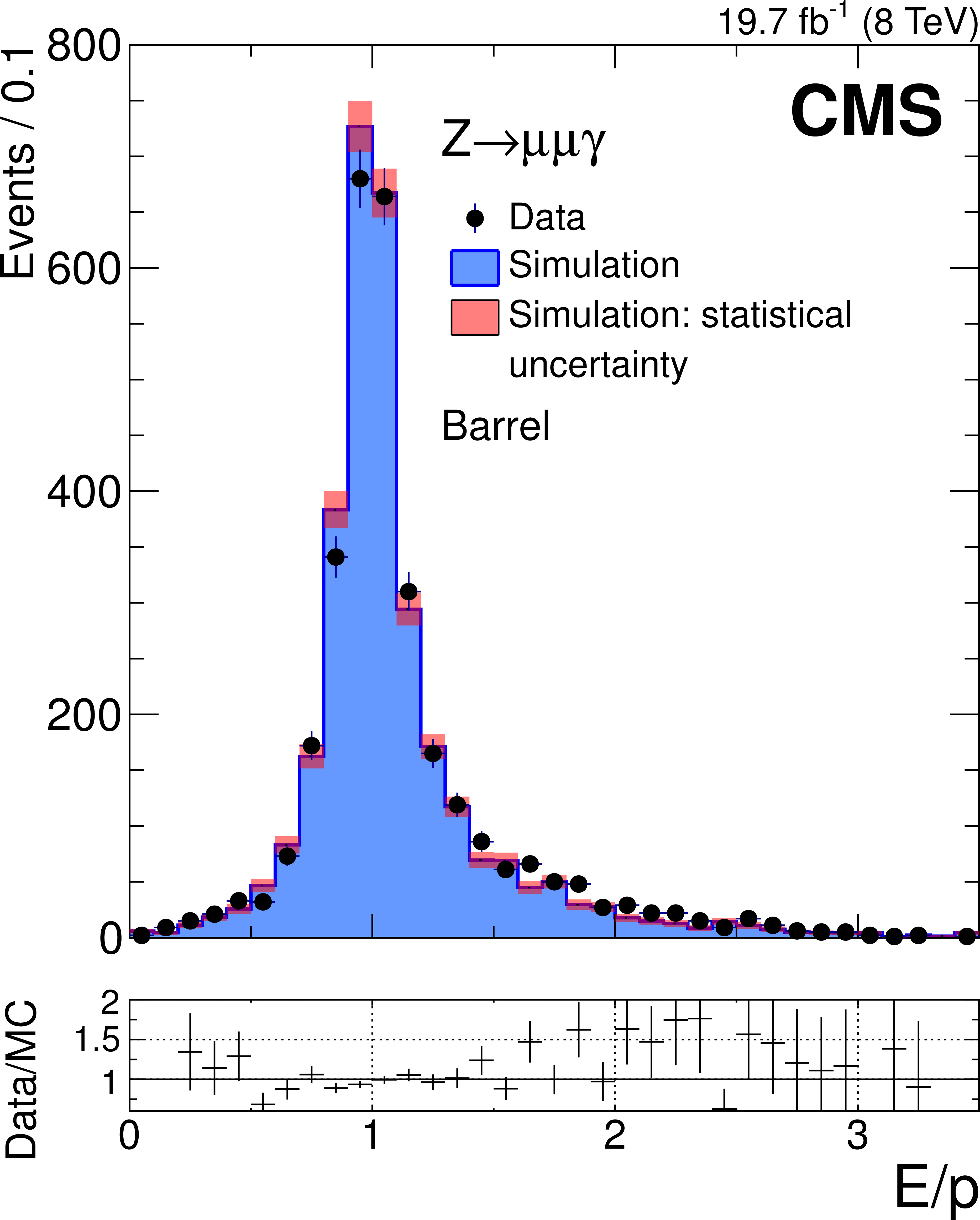
Figure 13-a:
Distribution of the $E/p$ ratio, where $E$ is the supercluster energy measured in the ECAL and $p$ is the total momentum measured from the track pair refitted with the conversion vertex constraint, for photons in $ { {\mathrm {Z}}\to {{\mu ^+}} {{\mu ^-}} {\gamma }} $ events in data (points with error bars) and simulation (histograms), separately for (left) barrel and (right) endcap. The simulated distributions are normalized to the number of entries in data. |
png pdf |
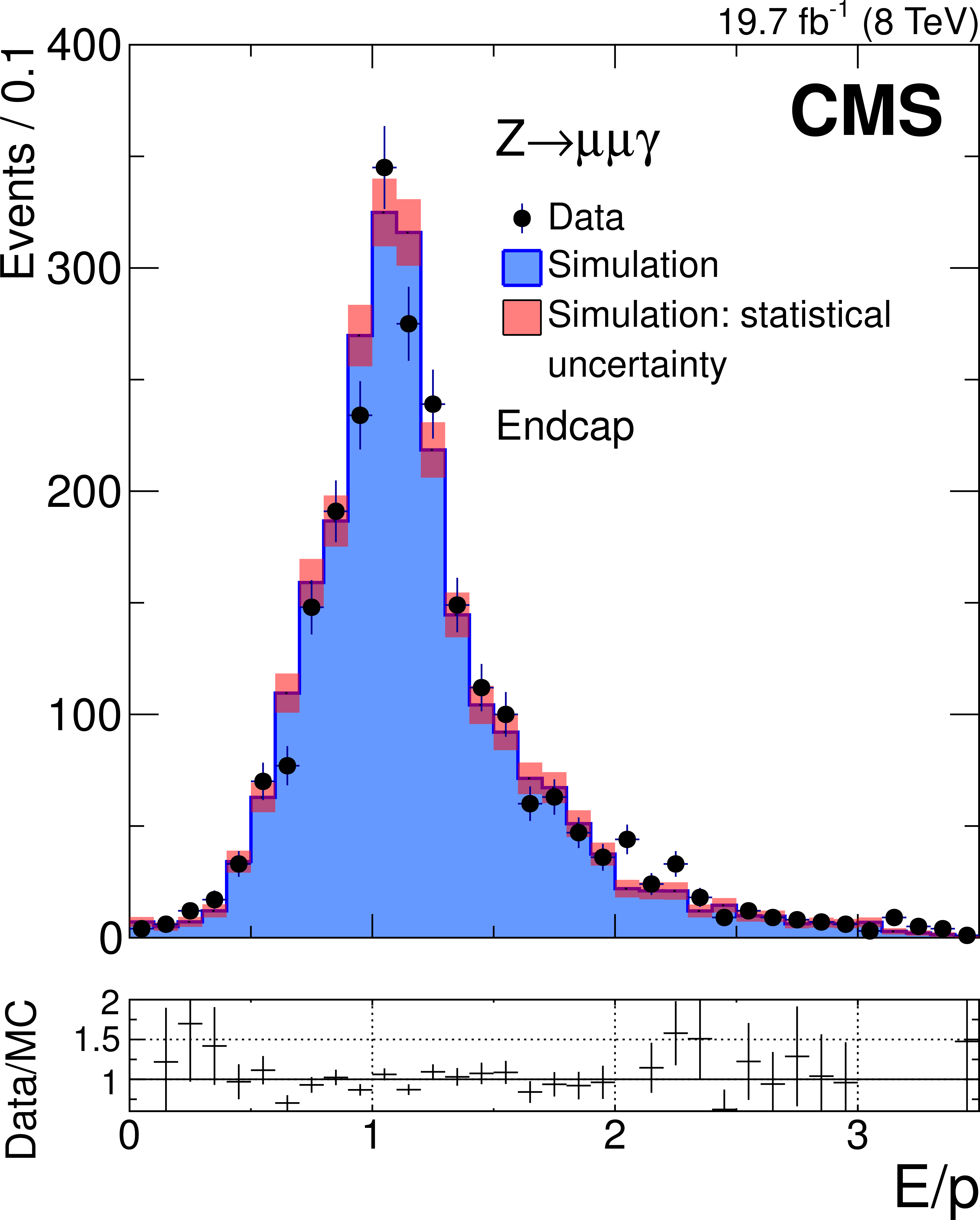
Figure 13-b:
Distribution of the $E/p$ ratio, where $E$ is the supercluster energy measured in the ECAL and $p$ is the total momentum measured from the track pair refitted with the conversion vertex constraint, for photons in $ { {\mathrm {Z}}\to {{\mu ^+}} {{\mu ^-}} {\gamma }} $ events in data (points with error bars) and simulation (histograms), separately for (left) barrel and (right) endcap. The simulated distributions are normalized to the number of entries in data. |

png pdf |
Figure 14-a:
(a) Distribution of the photon supercluster (absolute) pseudorapidity for events with reconstructed conversion vertices in data (points with error bars) and simulation (histograms). (b) Distribution of the conversion vertex radius for photons in the range $ {| \eta | }<1.4$ in data (points with error bars) and simulation (histograms). |
png pdf |
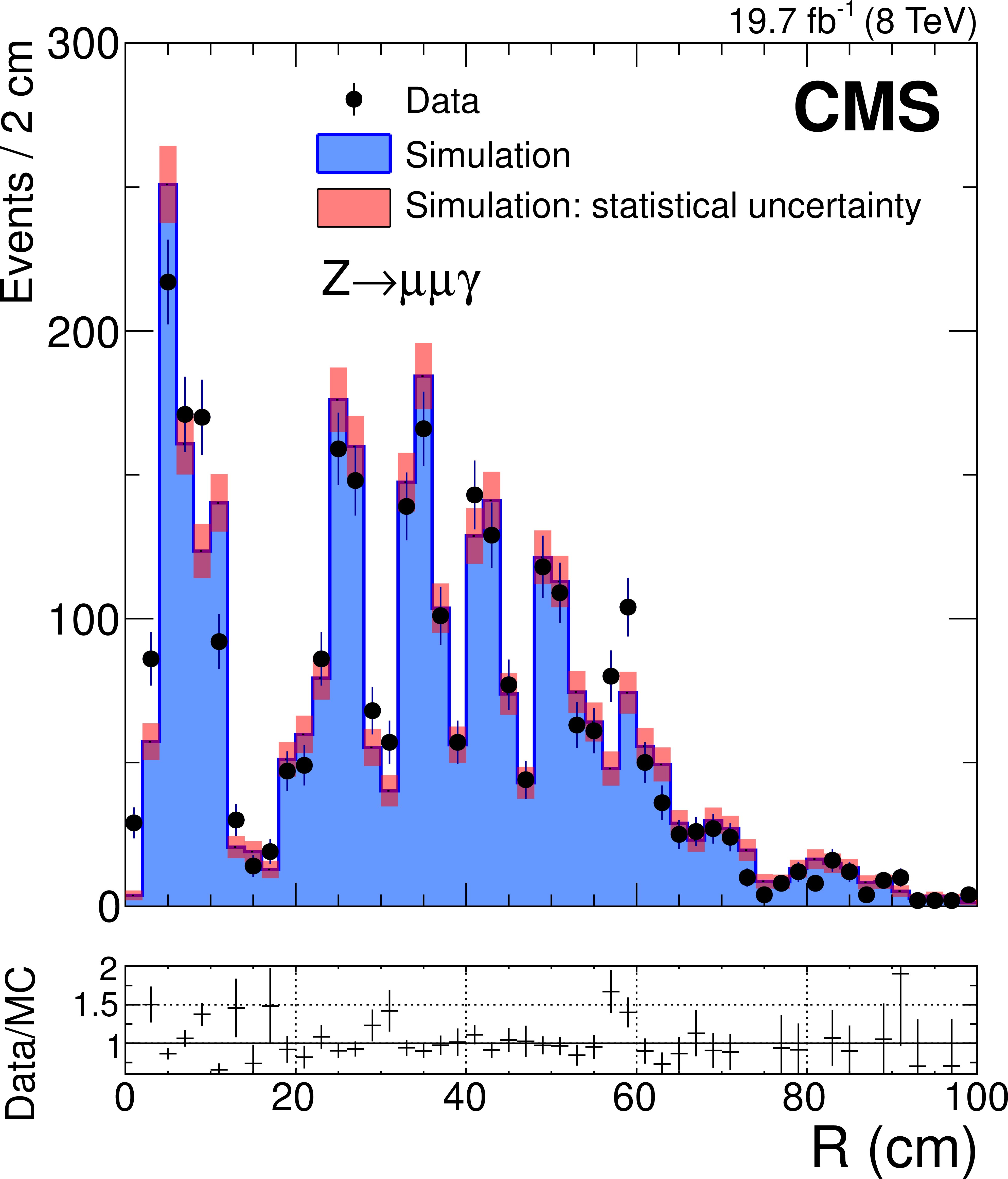
Figure 14-b:
(a) Distribution of the photon supercluster (absolute) pseudorapidity for events with reconstructed conversion vertices in data (points with error bars) and simulation (histograms). (b) Distribution of the conversion vertex radius for photons in the range $ {| \eta | }<1.4$ in data (points with error bars) and simulation (histograms). |
png pdf |
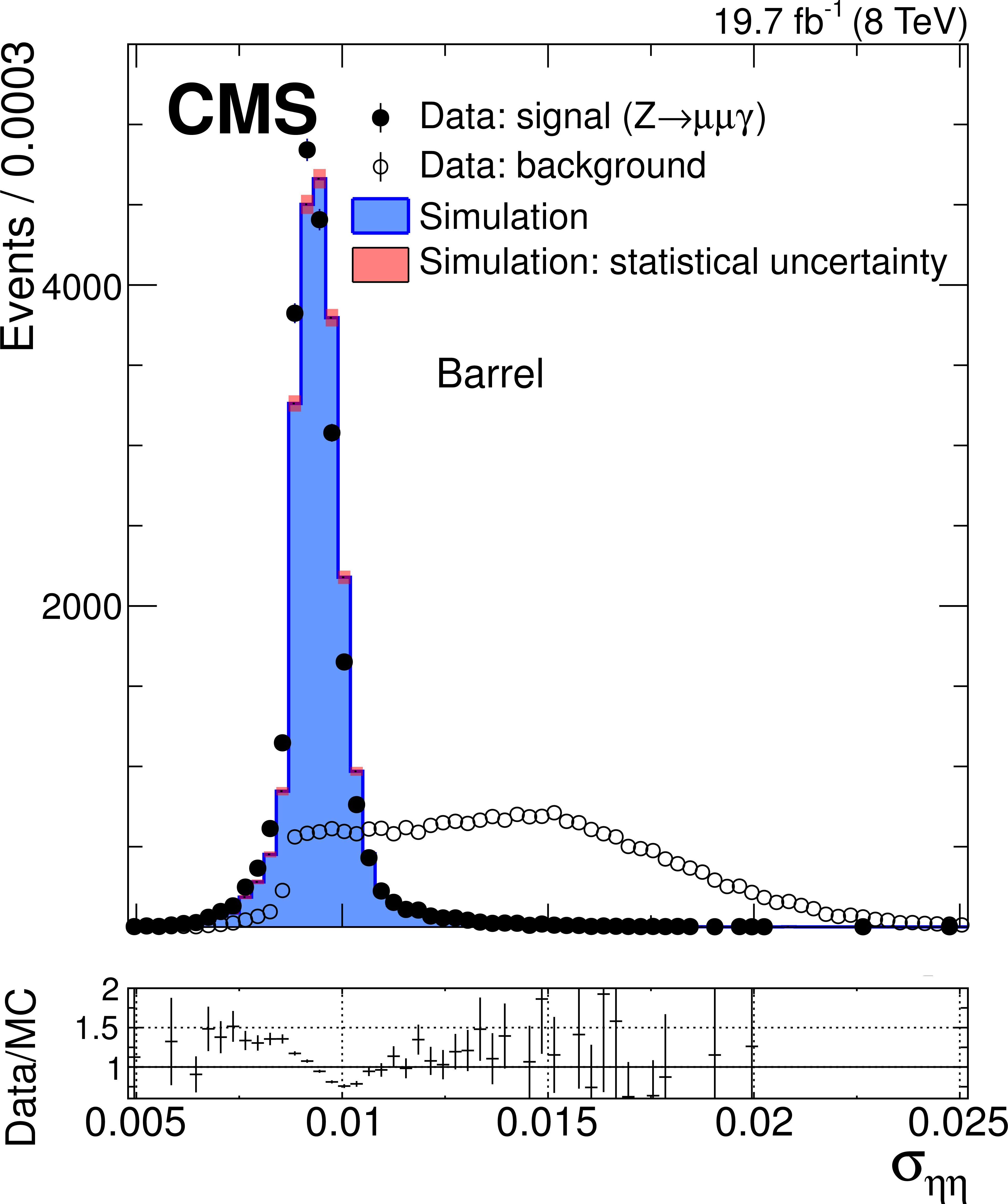
Figure 15-a:
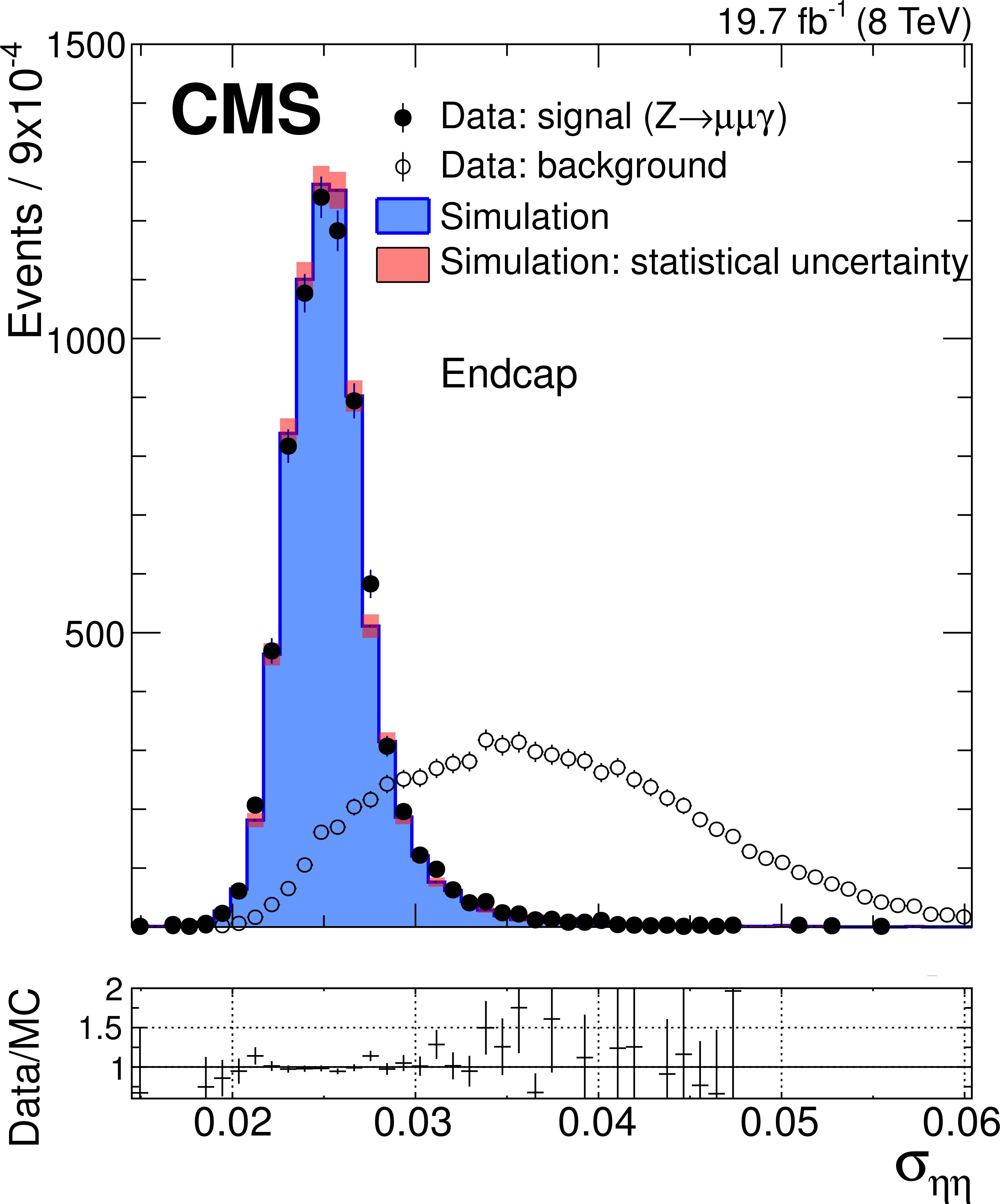
Distribution of the shower-shape variable, $ {\sigma _{\eta \eta }} $, for FSR photons in $ { {\mathrm {Z}}\to {{\mu ^+}} {{\mu ^-}} {\gamma }}$ events in data (solid circles) and simulation (histogram), and for background-dominated photon candidates in dimuon triggered events (open circles). The barrel and endcaps are shown separately. The simulated signal and background distributions are normalized to the number of signal photons in the data. The ratios between the photon signal distributions in data and simulation are shown in the bottom panels. |
png pdf |
Figure 15-b:
Distribution of the shower-shape variable, $ {\sigma _{\eta \eta }} $, for FSR photons in $ { {\mathrm {Z}}\to {{\mu ^+}} {{\mu ^-}} {\gamma }}$ events in data (solid circles) and simulation (histogram), and for background-dominated photon candidates in dimuon triggered events (open circles). The barrel and endcaps are shown separately. The simulated signal and background distributions are normalized to the number of signal photons in the data. The ratios between the photon signal distributions in data and simulation are shown in the bottom panels. |

png pdf |
Figure 16-a:
Mean value of the isolation variables for photons with $ {p_{\mathrm {T}}} > $ 50 GeV in $ {\gamma + \text {jet}}$ events, as a function of the number of reconstructed primary vertices, for events (a) before and (b) after being corrected for pileup using the $\rho $ variable. |

png pdf |
Figure 16-b:
Mean value of the isolation variables for photons with $ {p_{\mathrm {T}}} > $ 50 GeV in $ {\gamma + \text {jet}}$ events, as a function of the number of reconstructed primary vertices, for events (a) before and (b) after being corrected for pileup using the $\rho $ variable. |
png pdf |
Figure 17-a:
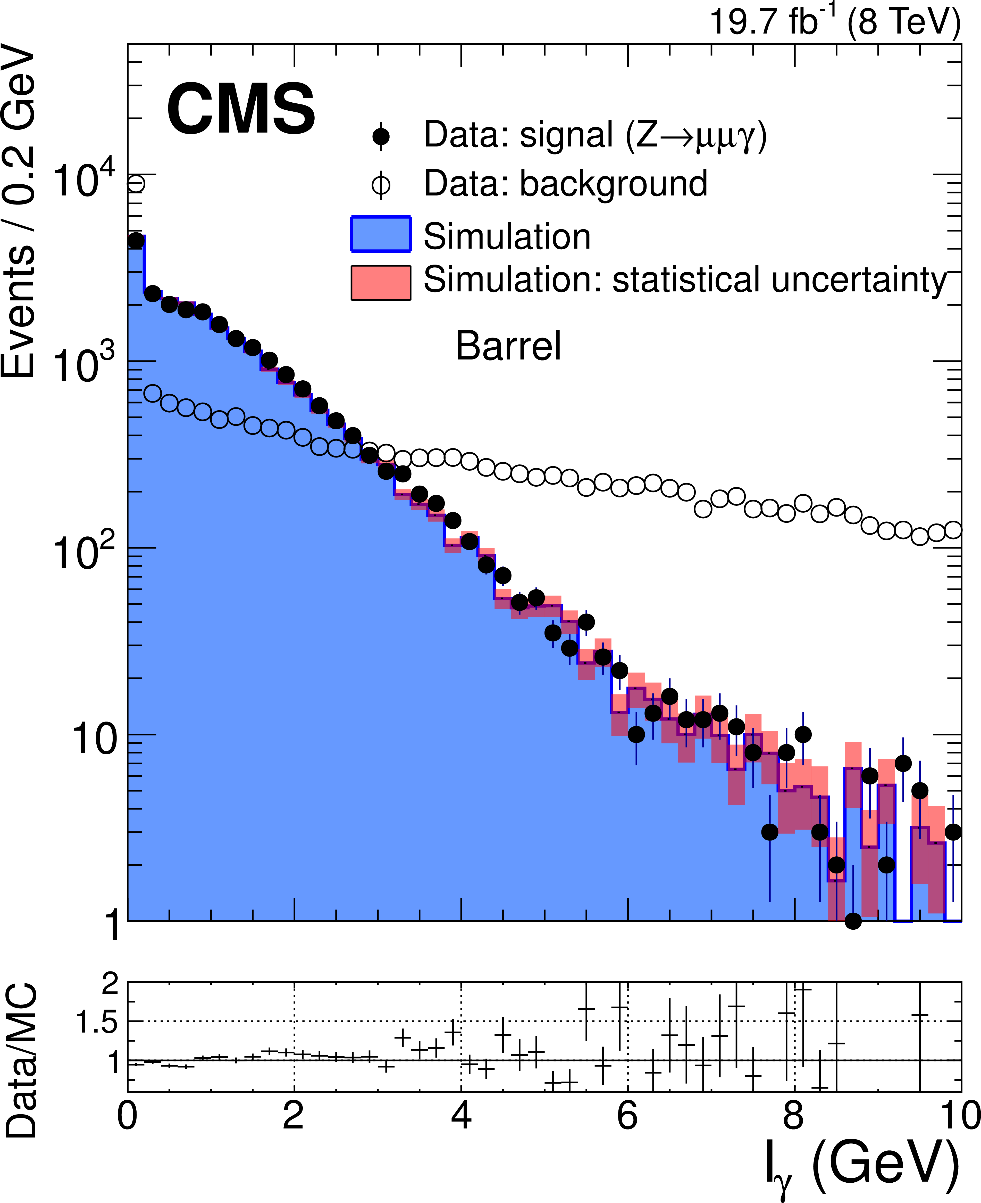
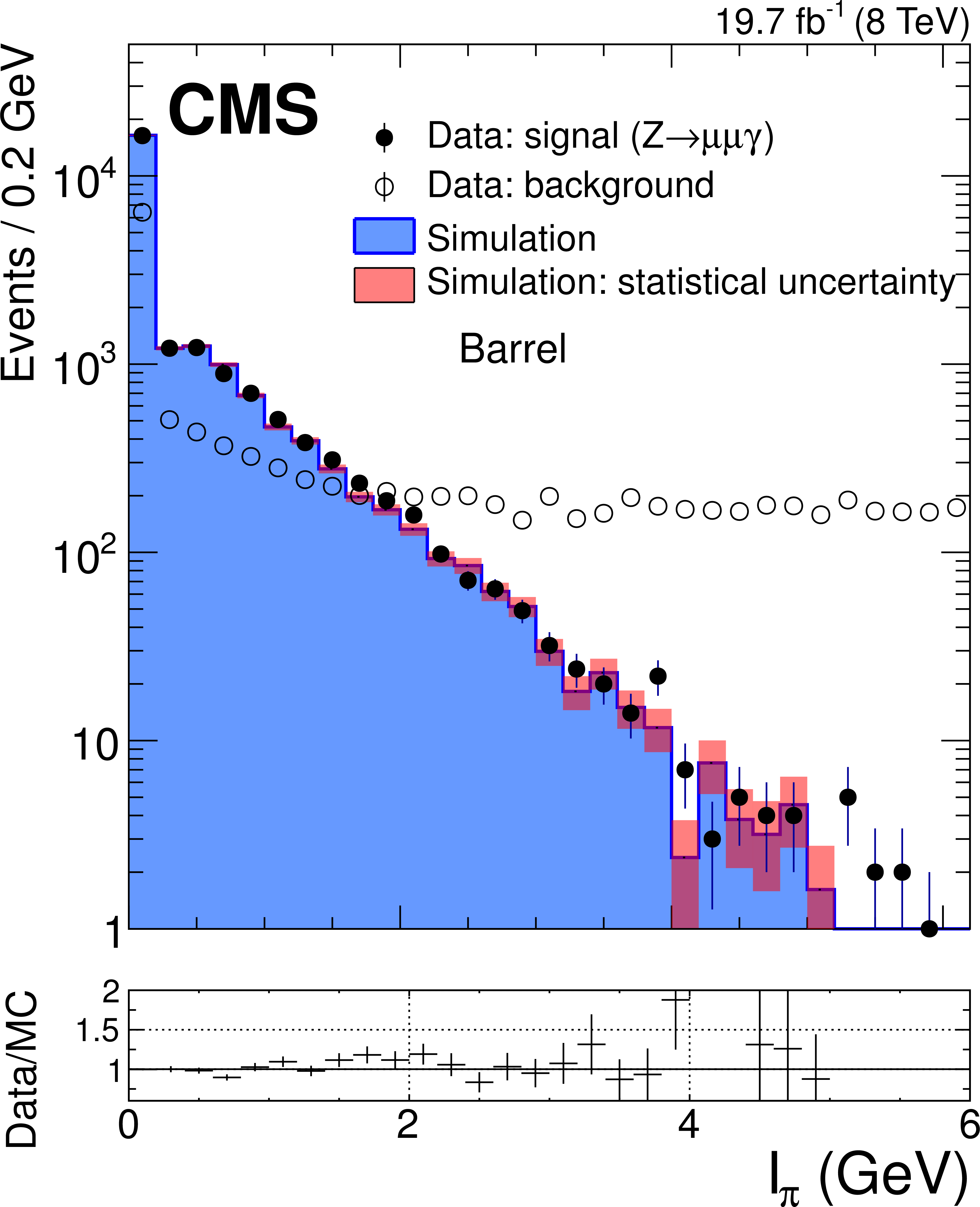
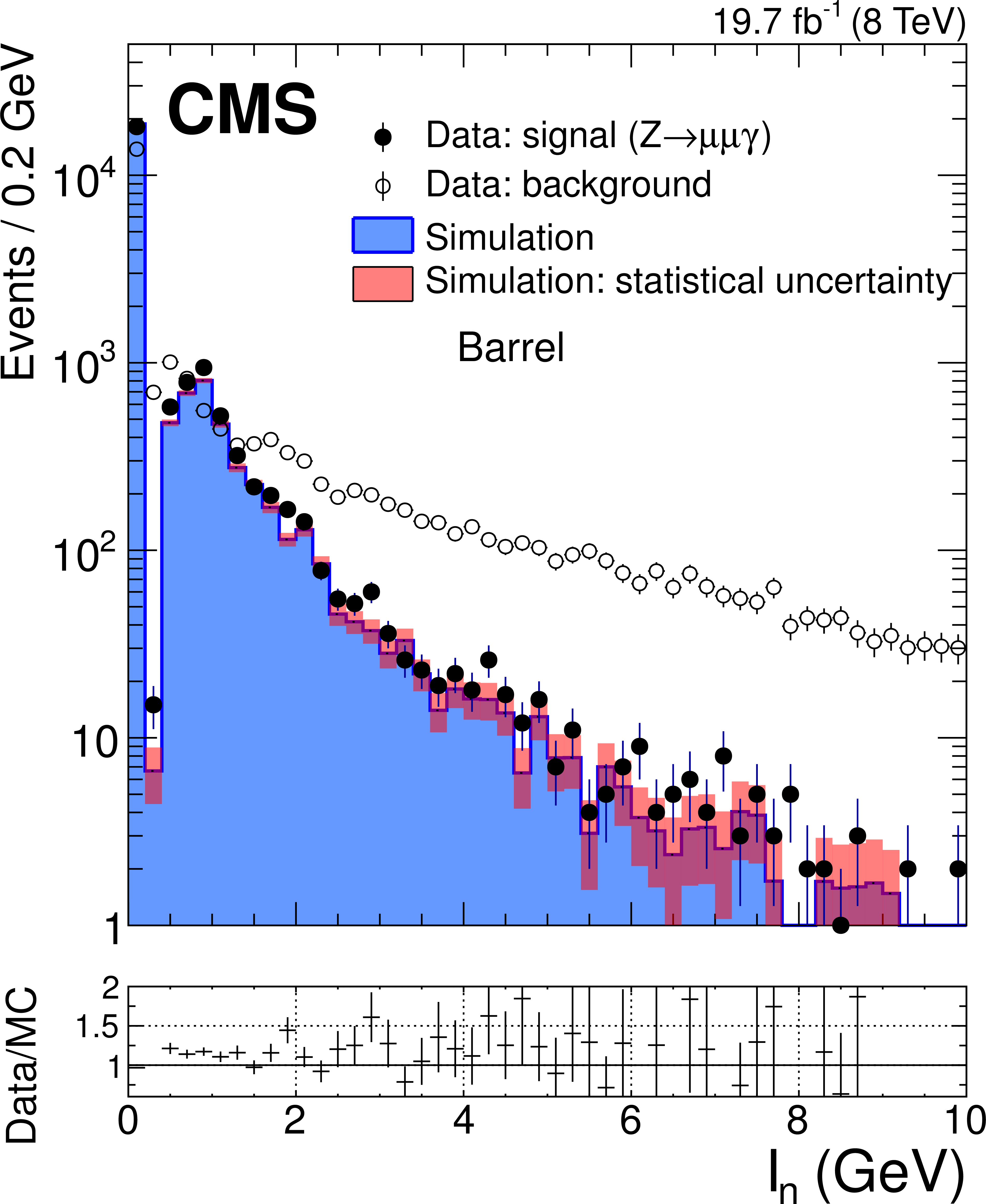
Distributions of the isolation variables: (top) $I_{\gamma }$, (bottom left) $I_\pi $, and (bottom right) $I_\text {n}$, constructed from particle-flow objects. The distributions are shown for FSR photons from $ { {\mathrm {Z}}\to {{\mu ^+}} {{\mu ^-}} {\gamma }} $ events in data (solid circles) and simulation (histogram) and for background-dominated photon candidates in dimuon triggered events (open circles). The simulated signal and background distributions are normalized to the number of signal photons in data. The ratios between the photon signal distributions in data and simulation are shown in the bottom panels. |
png pdf |
Figure 17-b:
Distributions of the isolation variables: (top) $I_{\gamma }$, (bottom left) $I_\pi $, and (bottom right) $I_\text {n}$, constructed from particle-flow objects. The distributions are shown for FSR photons from $ { {\mathrm {Z}}\to {{\mu ^+}} {{\mu ^-}} {\gamma }} $ events in data (solid circles) and simulation (histogram) and for background-dominated photon candidates in dimuon triggered events (open circles). The simulated signal and background distributions are normalized to the number of signal photons in data. The ratios between the photon signal distributions in data and simulation are shown in the bottom panels. |
png pdf |
Figure 17-c:
Distributions of the isolation variables: (top) $I_{\gamma }$, (bottom left) $I_\pi $, and (bottom right) $I_\text {n}$, constructed from particle-flow objects. The distributions are shown for FSR photons from $ { {\mathrm {Z}}\to {{\mu ^+}} {{\mu ^-}} {\gamma }} $ events in data (solid circles) and simulation (histogram) and for background-dominated photon candidates in dimuon triggered events (open circles). The simulated signal and background distributions are normalized to the number of signal photons in data. The ratios between the photon signal distributions in data and simulation are shown in the bottom panels. |
png pdf |
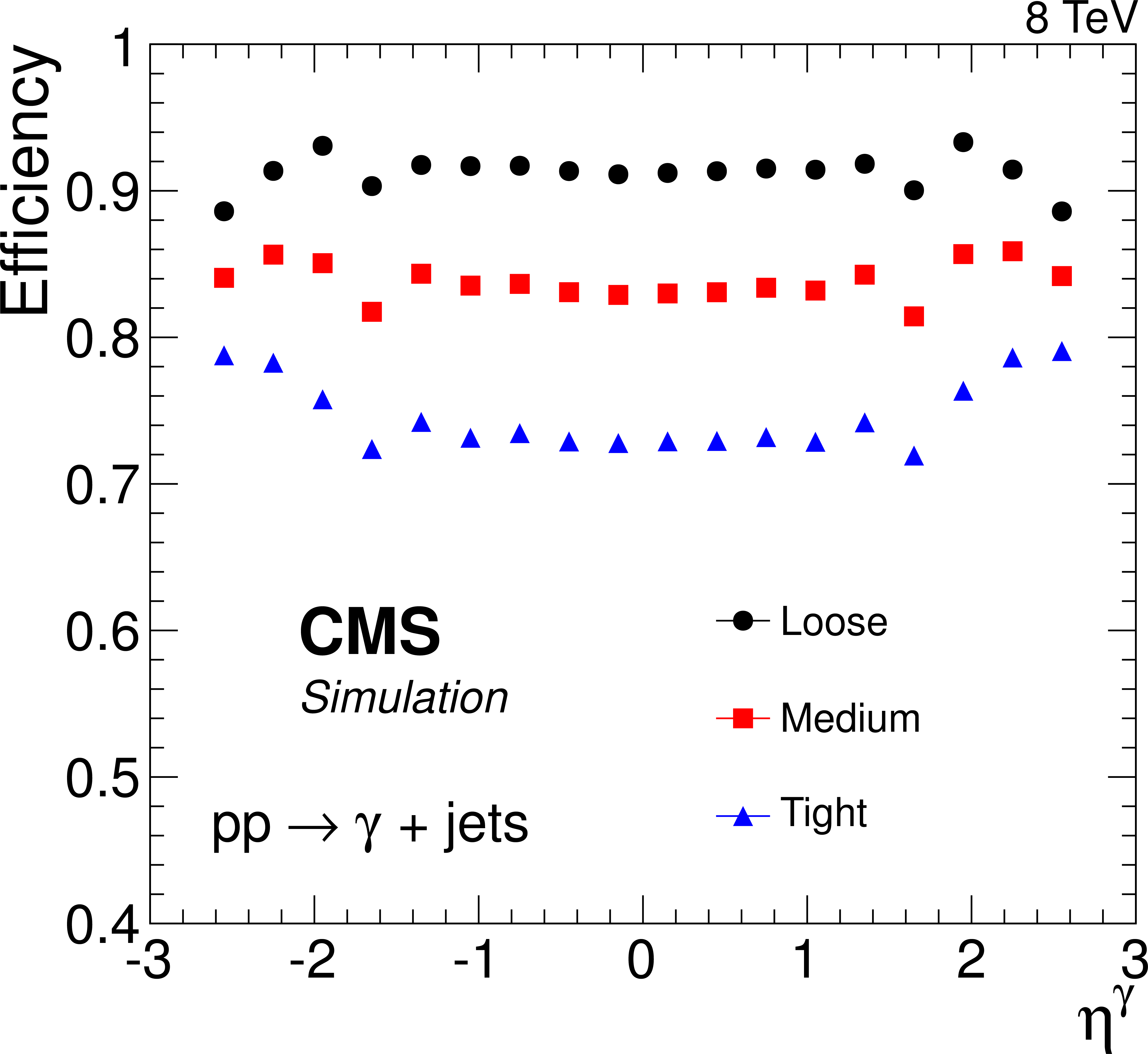
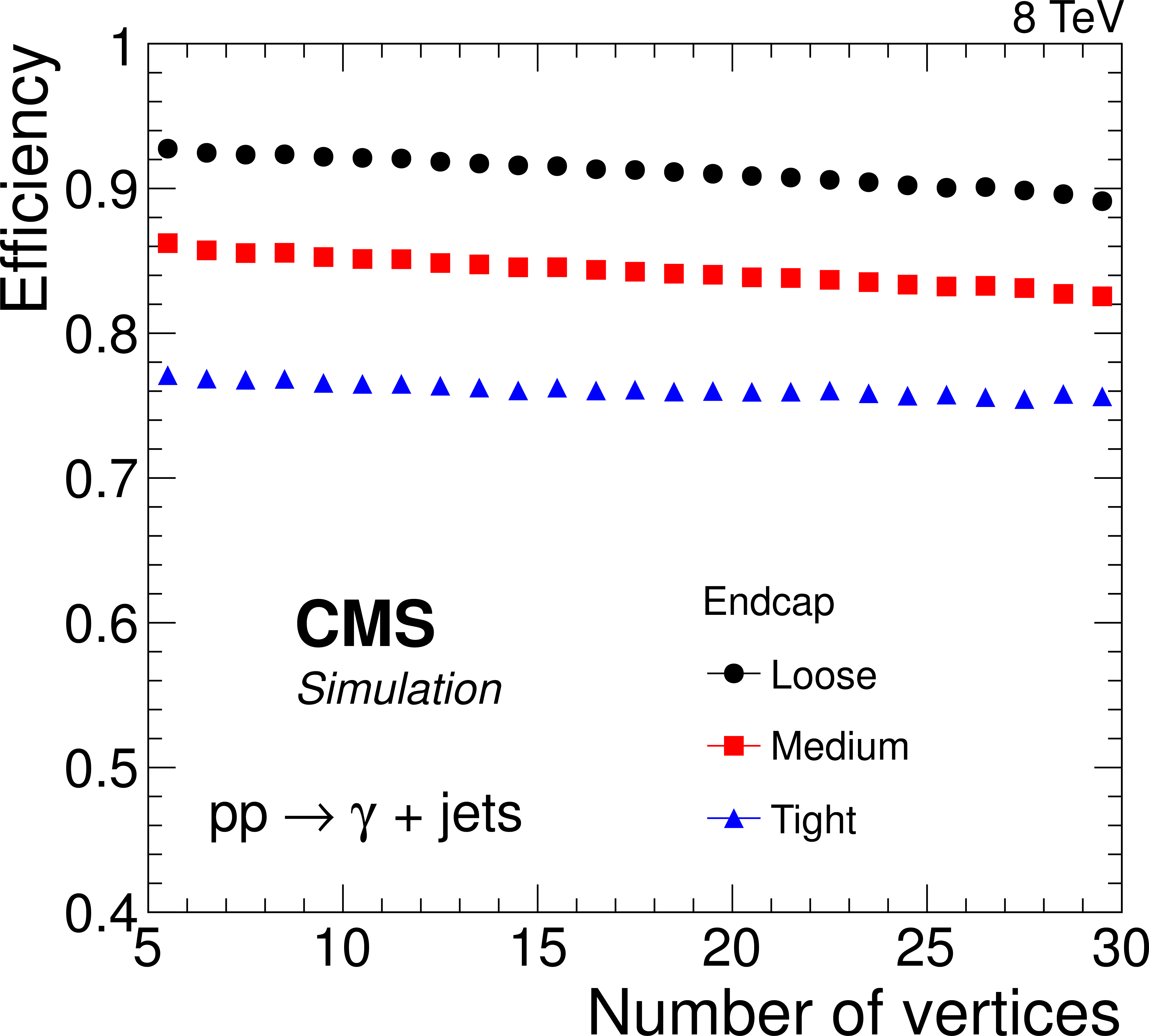
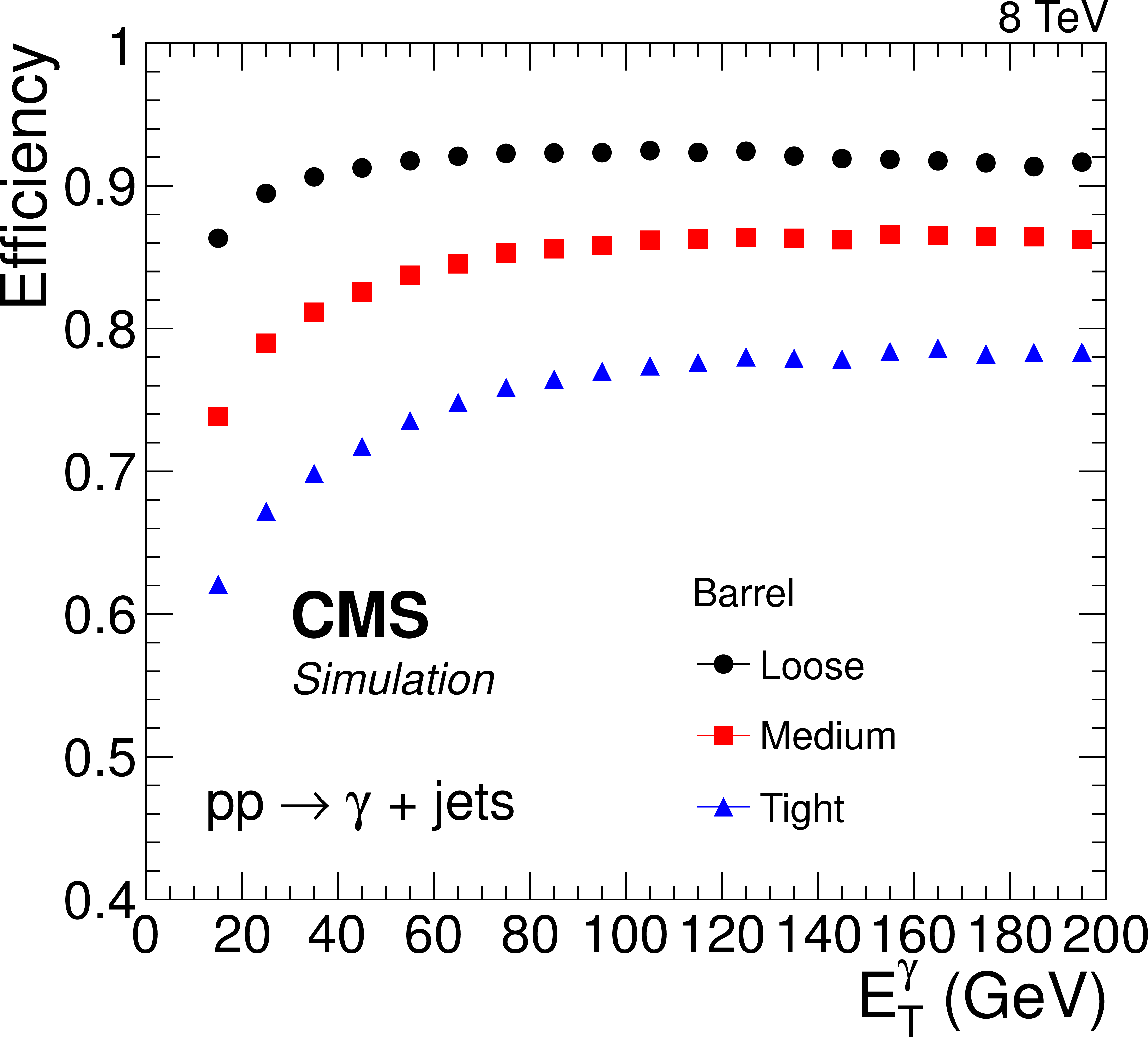
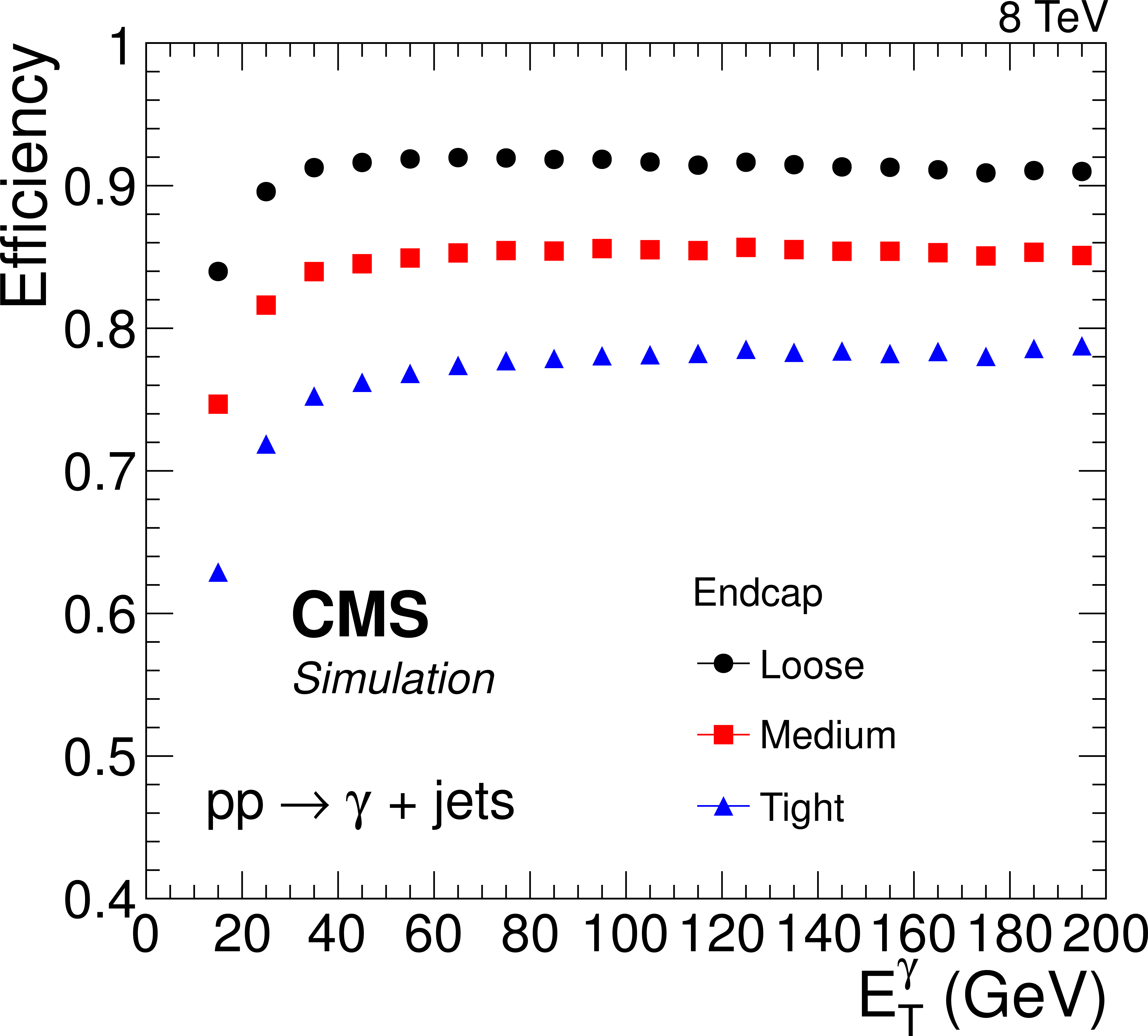
Figure 18-a:
Efficiency of photon identification based on sequential requirements in simulated $ {\gamma + \text {jet}}$ events for three different working points, as a function of the (top) photon pseudorapidity, (middle) number of pileup vertices, and (bottom) photon transverse momentum. The efficiencies shown include the electron veto requirement. |

png pdf |
Figure 18-b:
Efficiency of photon identification based on sequential requirements in simulated $ {\gamma + \text {jet}}$ events for three different working points, as a function of the (top) photon pseudorapidity, (middle) number of pileup vertices, and (bottom) photon transverse momentum. The efficiencies shown include the electron veto requirement. |
png pdf |
Figure 18-c:
Efficiency of photon identification based on sequential requirements in simulated $ {\gamma + \text {jet}}$ events for three different working points, as a function of the (top) photon pseudorapidity, (middle) number of pileup vertices, and (bottom) photon transverse momentum. The efficiencies shown include the electron veto requirement. |
png pdf |
Figure 18-d:
Efficiency of photon identification based on sequential requirements in simulated $ {\gamma + \text {jet}}$ events for three different working points, as a function of the (top) photon pseudorapidity, (middle) number of pileup vertices, and (bottom) photon transverse momentum. The efficiencies shown include the electron veto requirement. |
png pdf |
Figure 18-e:
Efficiency of photon identification based on sequential requirements in simulated $ {\gamma + \text {jet}}$ events for three different working points, as a function of the (top) photon pseudorapidity, (middle) number of pileup vertices, and (bottom) photon transverse momentum. The efficiencies shown include the electron veto requirement. |
png pdf |
Figure 19-a:
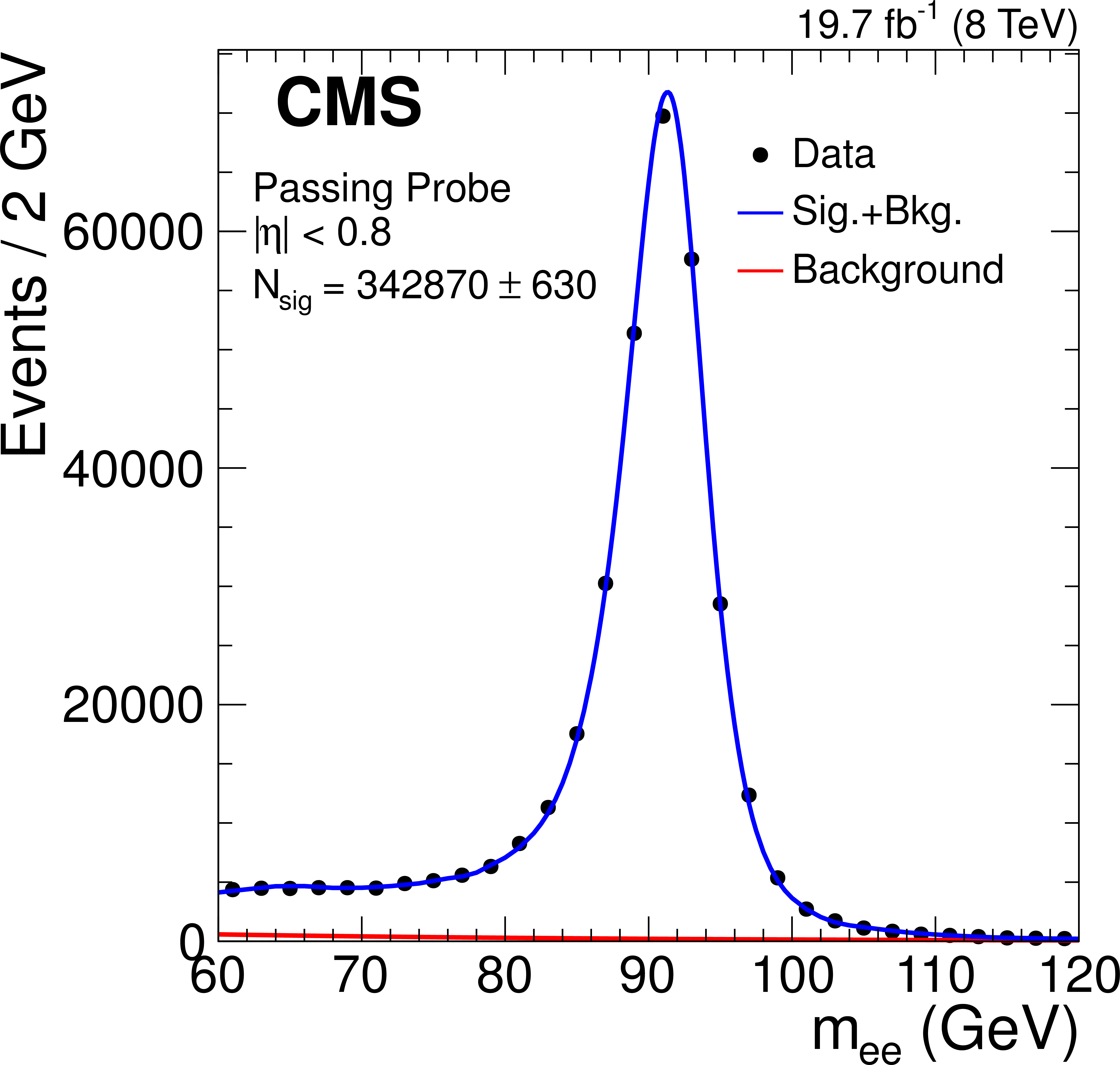
Example of fits to the $ { {\mathrm {Z}}\to {\mathrm {e}^+} {\mathrm {e}^-}} $ invariant mass distribution for (left) passing and (right) failing probes, in the transverse momentum range $20< {p_{\mathrm {T}}} <$ 30 GeV and $ {| \eta | } <$ 0.8. |
png pdf |
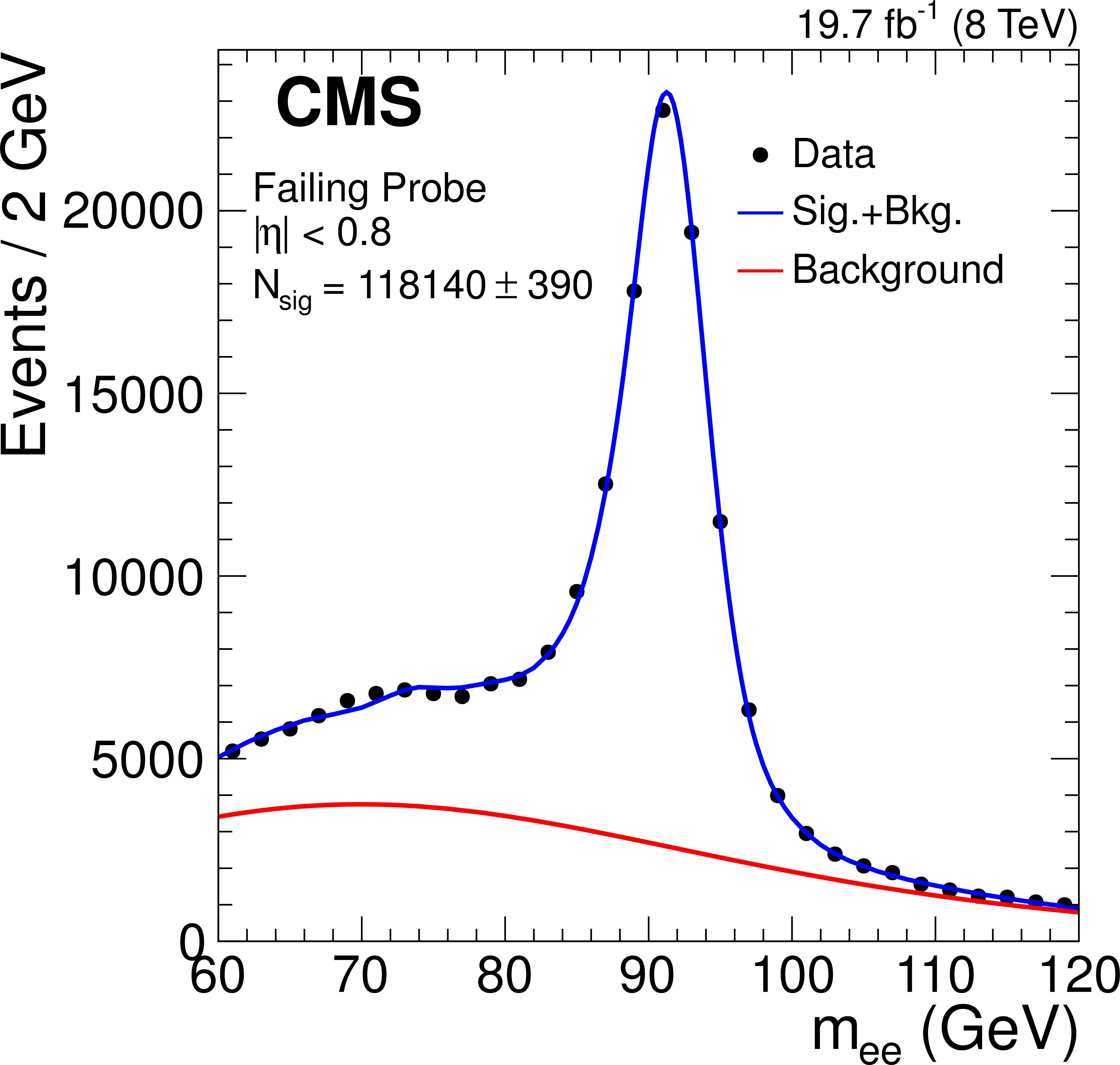
Figure 19-b:
Example of fits to the $ { {\mathrm {Z}}\to {\mathrm {e}^+} {\mathrm {e}^-}} $ invariant mass distribution for (left) passing and (right) failing probes, in the transverse momentum range $20< {p_{\mathrm {T}}} <$ 30 GeV and $ {| \eta | } <$ 0.8. |
png pdf |
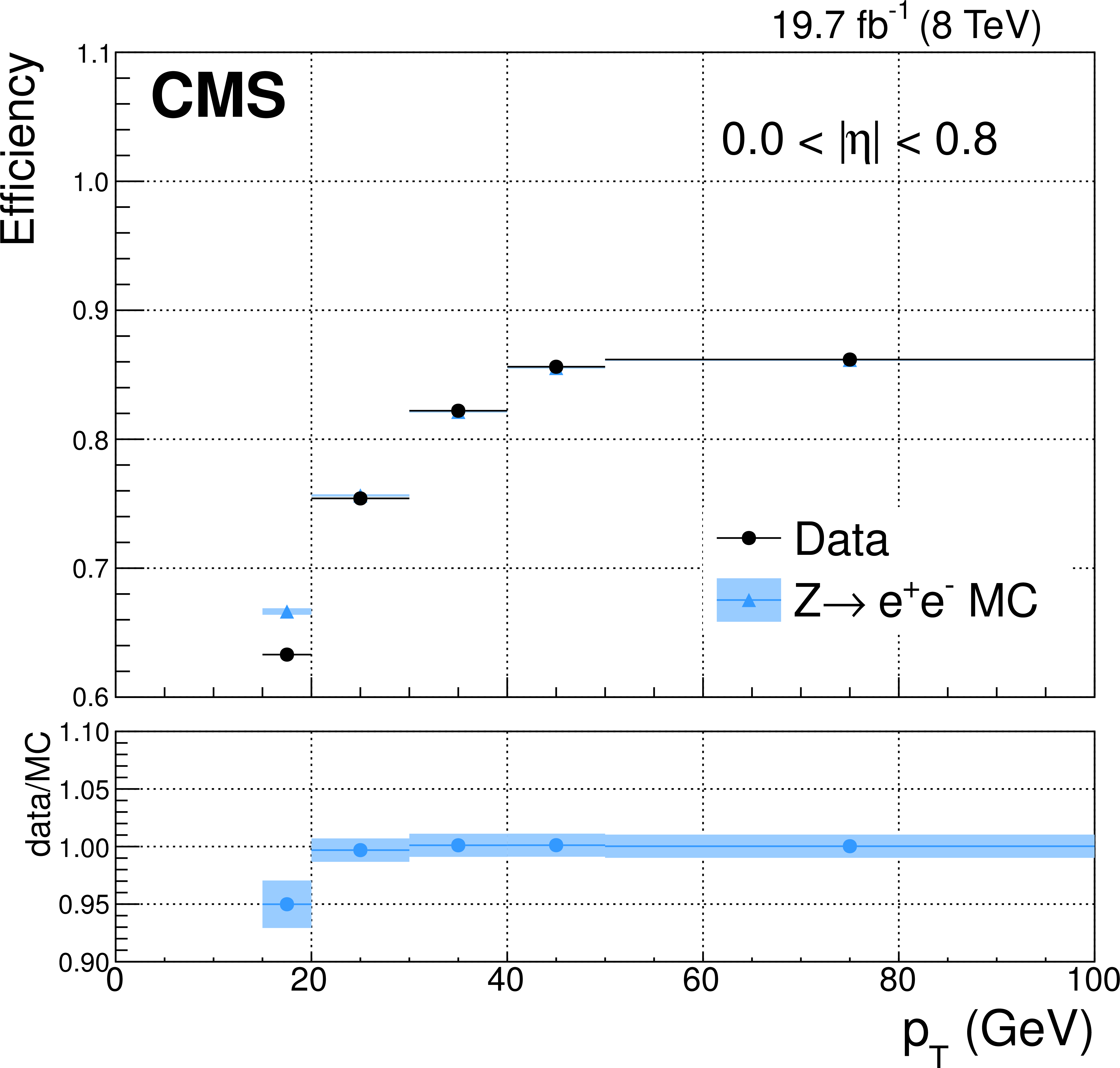
Figure 20-a:
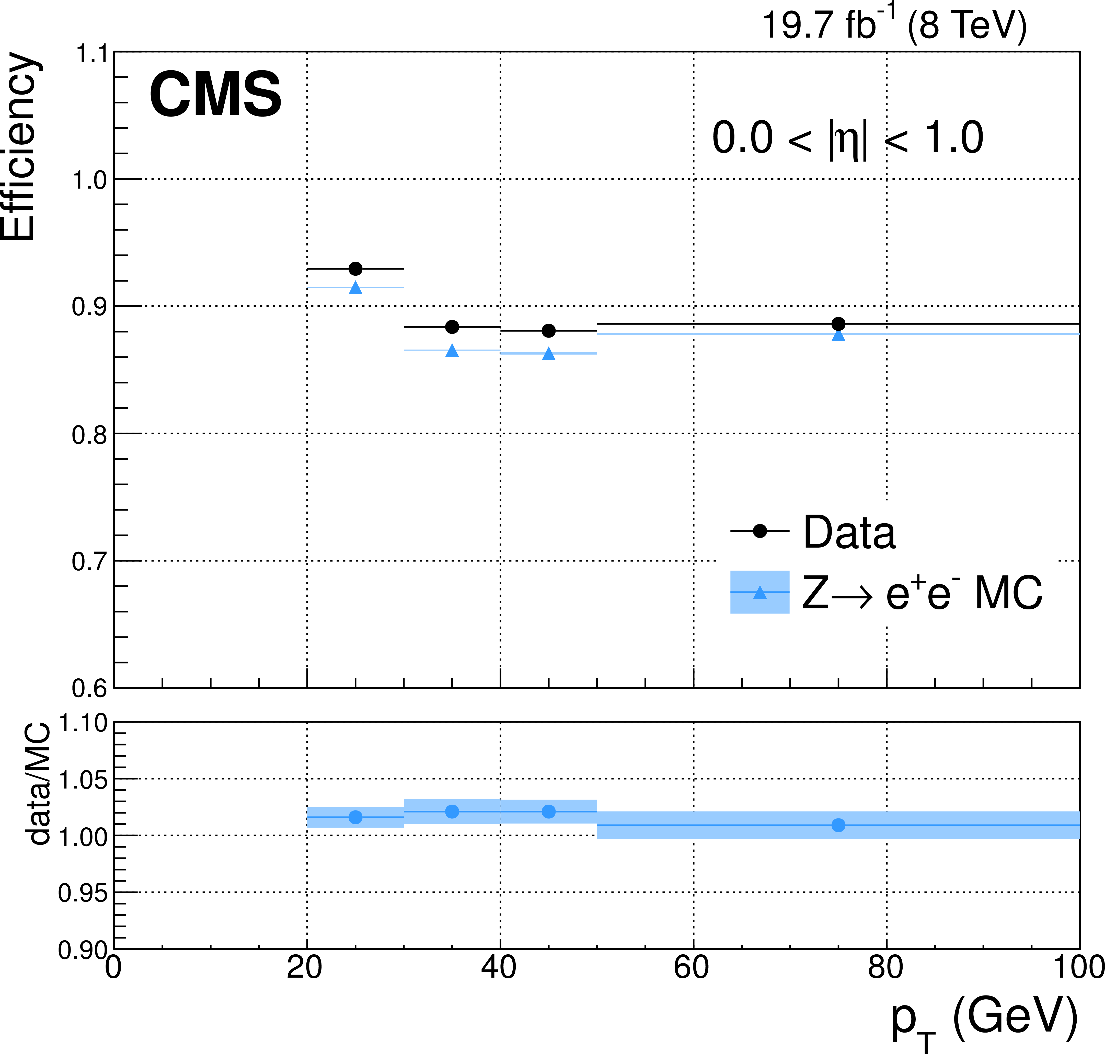
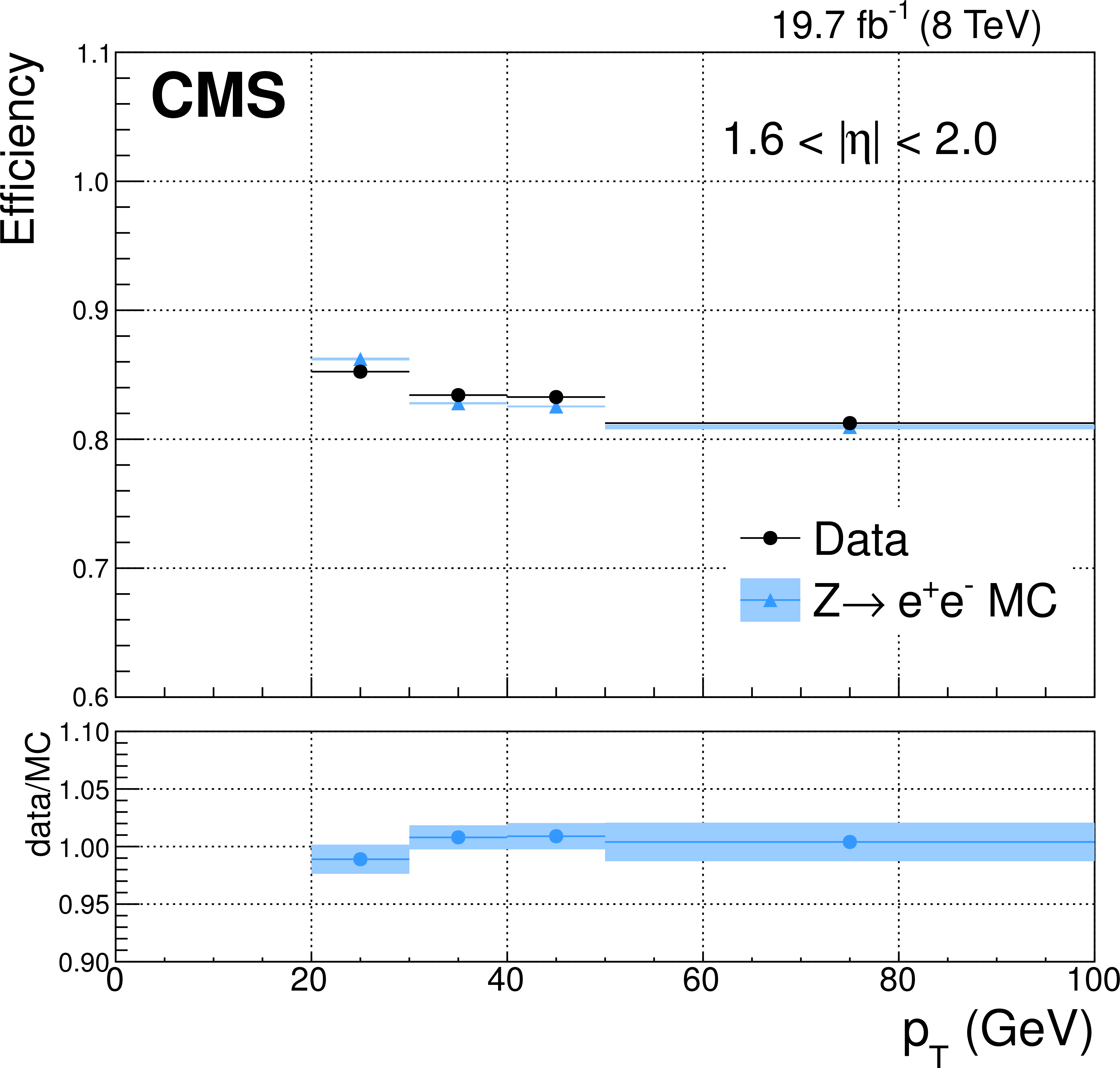
Comparison of the selection efficiency as a function of photon transverse momentum in data (circles) and simulation (triangles) for the identification based on sequential requirements for (left) $ {| \eta | } < 0.8$ and (right) $1.6 < {| \eta | } < 2$. Statistical and systematic uncertainties are respectively shown by the error bars and shaded bands. The horizontal error bars mark the full width of the $ {p_{\mathrm {T}}} $ bins in which the measurements are made, and the data points are plotted at the centre of each bin. The ratios of efficiencies in data and simulation are shown in the bottom panels. |
png pdf |
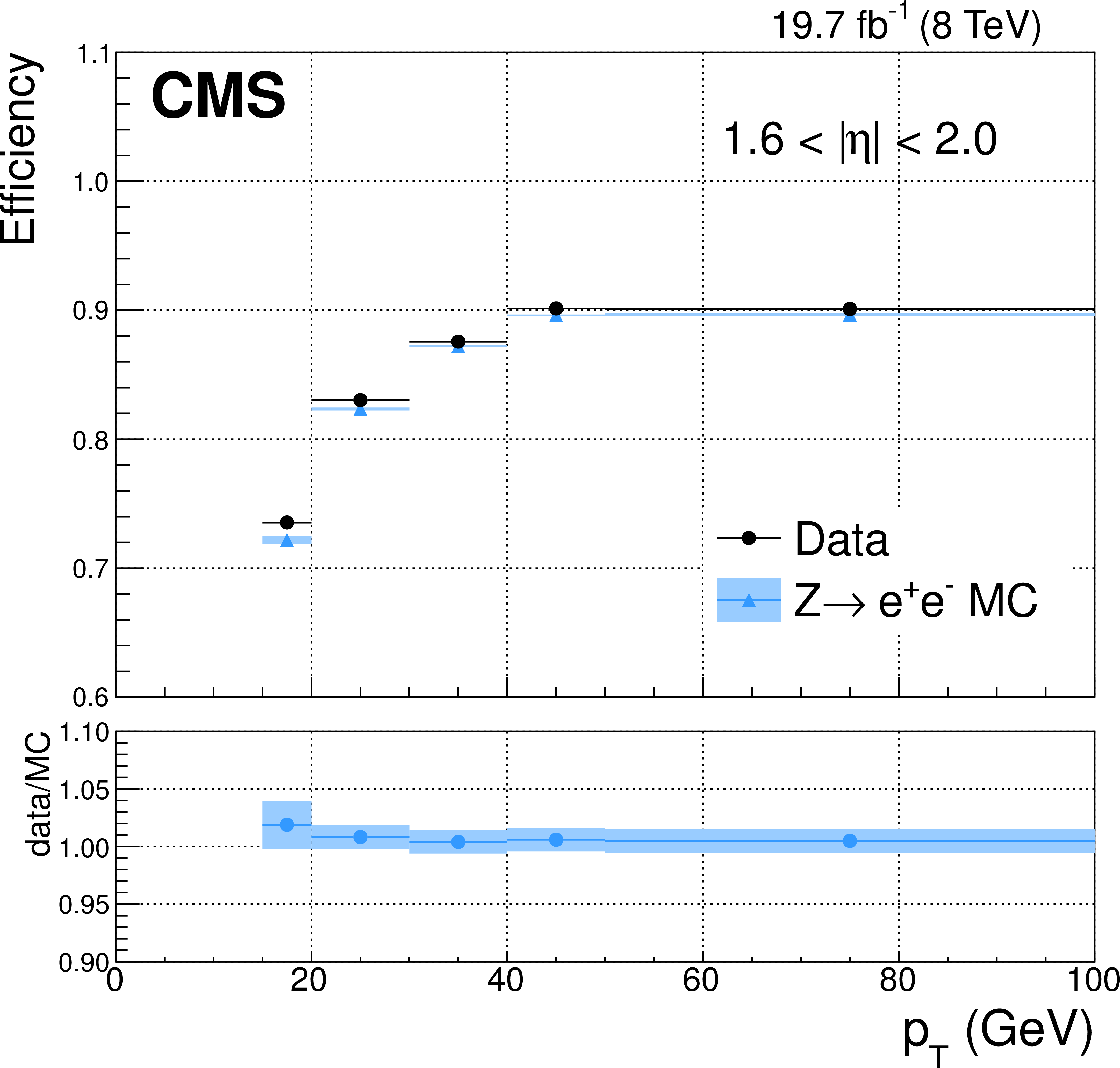
Figure 20-b:
Comparison of the selection efficiency as a function of photon transverse momentum in data (circles) and simulation (triangles) for the identification based on sequential requirements for (left) $ {| \eta | } < 0.8$ and (right) $1.6 < {| \eta | } < 2$. Statistical and systematic uncertainties are respectively shown by the error bars and shaded bands. The horizontal error bars mark the full width of the $ {p_{\mathrm {T}}} $ bins in which the measurements are made, and the data points are plotted at the centre of each bin. The ratios of efficiencies in data and simulation are shown in the bottom panels. |
png pdf |
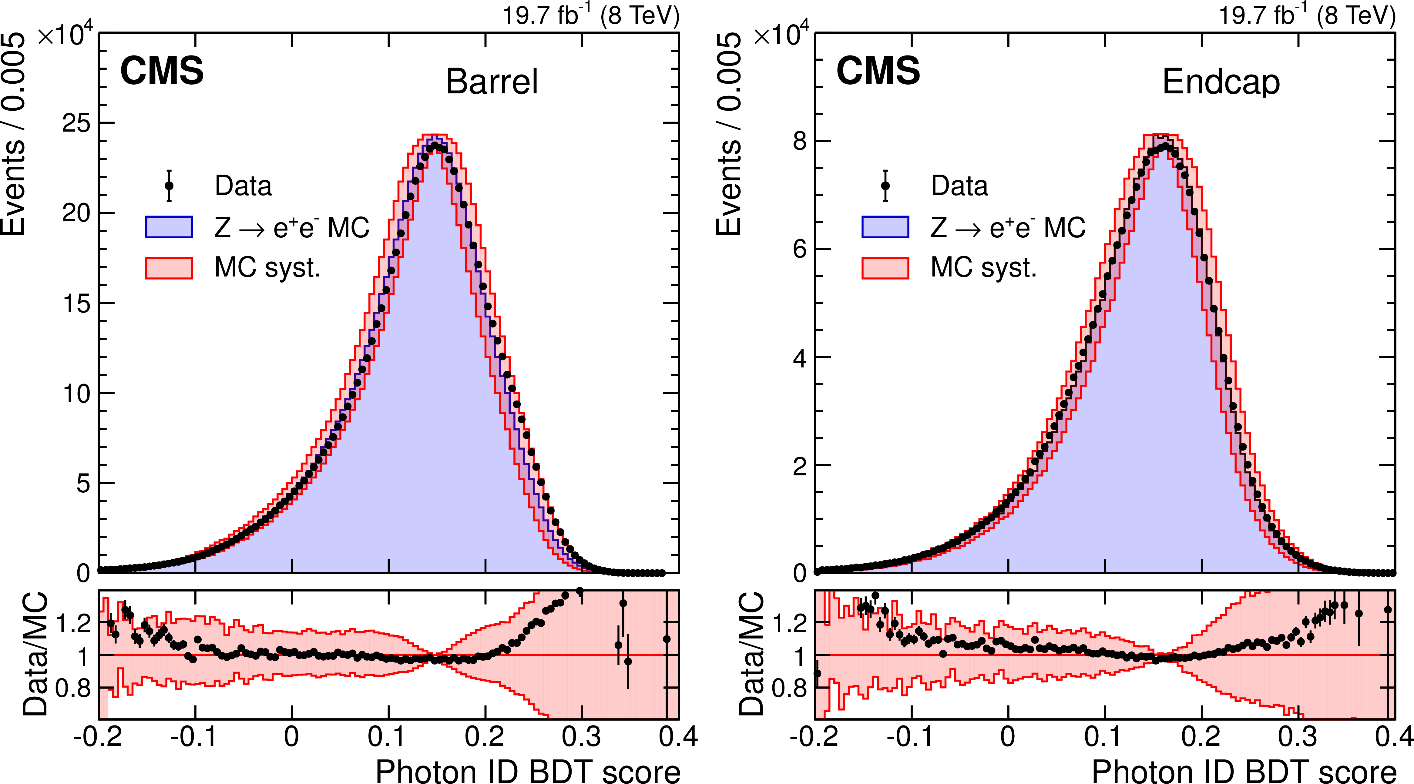
Figure 21:
Photon identification BDT score for electrons from $ { {\mathrm {Z}}\to {\mathrm {e}^+} {\mathrm {e}^-}} $ reconstructed as photons in the (a) ECAL barrel and (b) endcap. The distributions in data are compared to those in simulated Drell--Yan events. The hatched bands correspond to a shift of $\pm $0.01 applied to the score in simulated events. The corresponding ratios of data to simulation are shown in the bottom panels. |
png pdf |
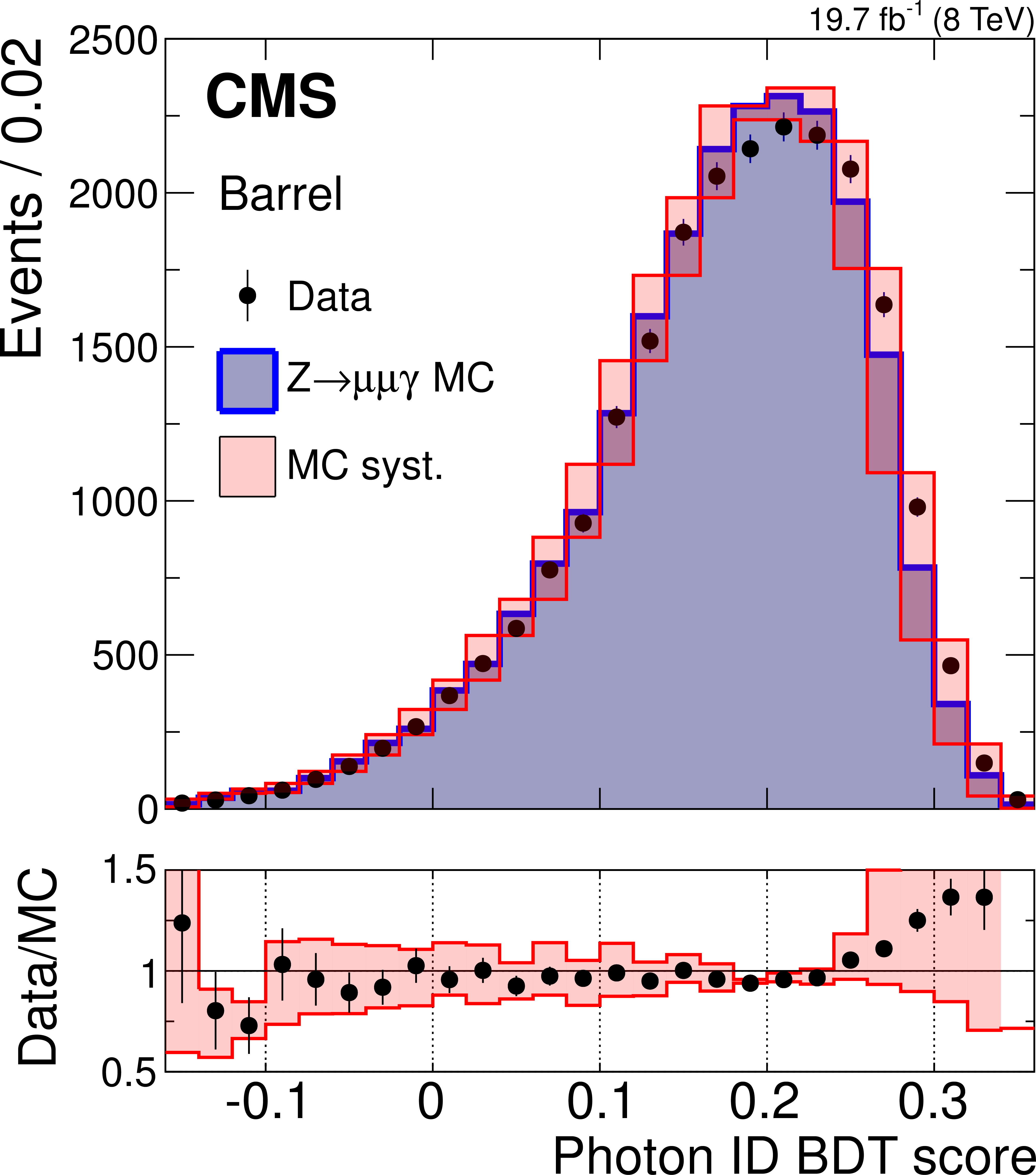
Figure 22-a:
Identification BDT estimator for photons from $ { {\mathrm {Z}}\to {{\mu ^+}} {{\mu ^-}} {\gamma }} $ with transverse momentum above 20 GeV . Data (points with error bars) are compared to $ { {\mathrm {Z}}\to {{\mu ^+}} {{\mu ^-}} {\gamma }} $ events selected in Drell--Yan simulation (histograms). The hashed bands correspond to a shift of $\pm $0.01 applied to the estimator value in simulation. The corresponding ratios of data to simulation are shown in the bottom panels. |
png pdf |
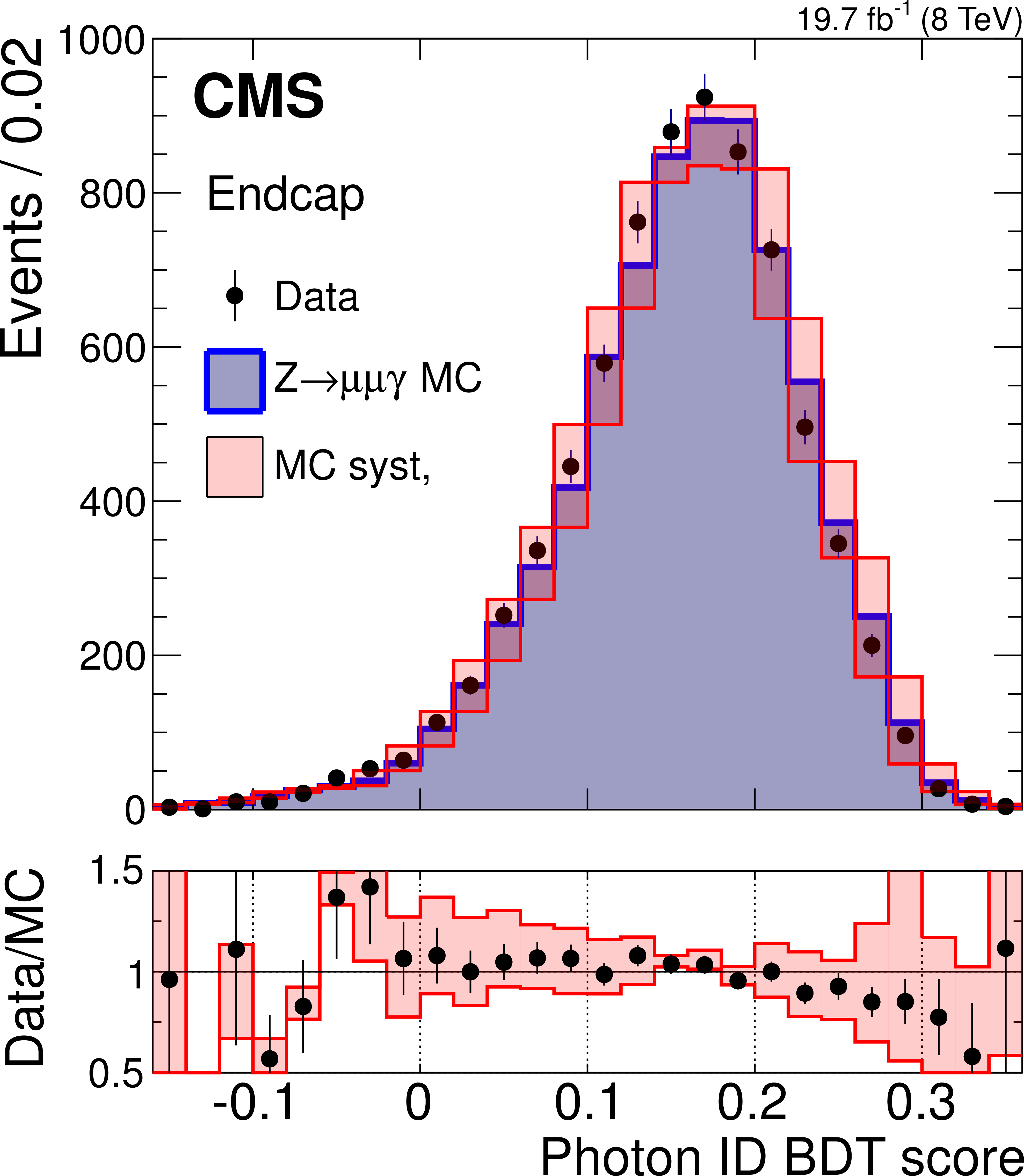
Figure 22-b:
Identification BDT estimator for photons from $ { {\mathrm {Z}}\to {{\mu ^+}} {{\mu ^-}} {\gamma }} $ with transverse momentum above 20 GeV . Data (points with error bars) are compared to $ { {\mathrm {Z}}\to {{\mu ^+}} {{\mu ^-}} {\gamma }} $ events selected in Drell--Yan simulation (histograms). The hashed bands correspond to a shift of $\pm $0.01 applied to the estimator value in simulation. The corresponding ratios of data to simulation are shown in the bottom panels. |
png pdf |
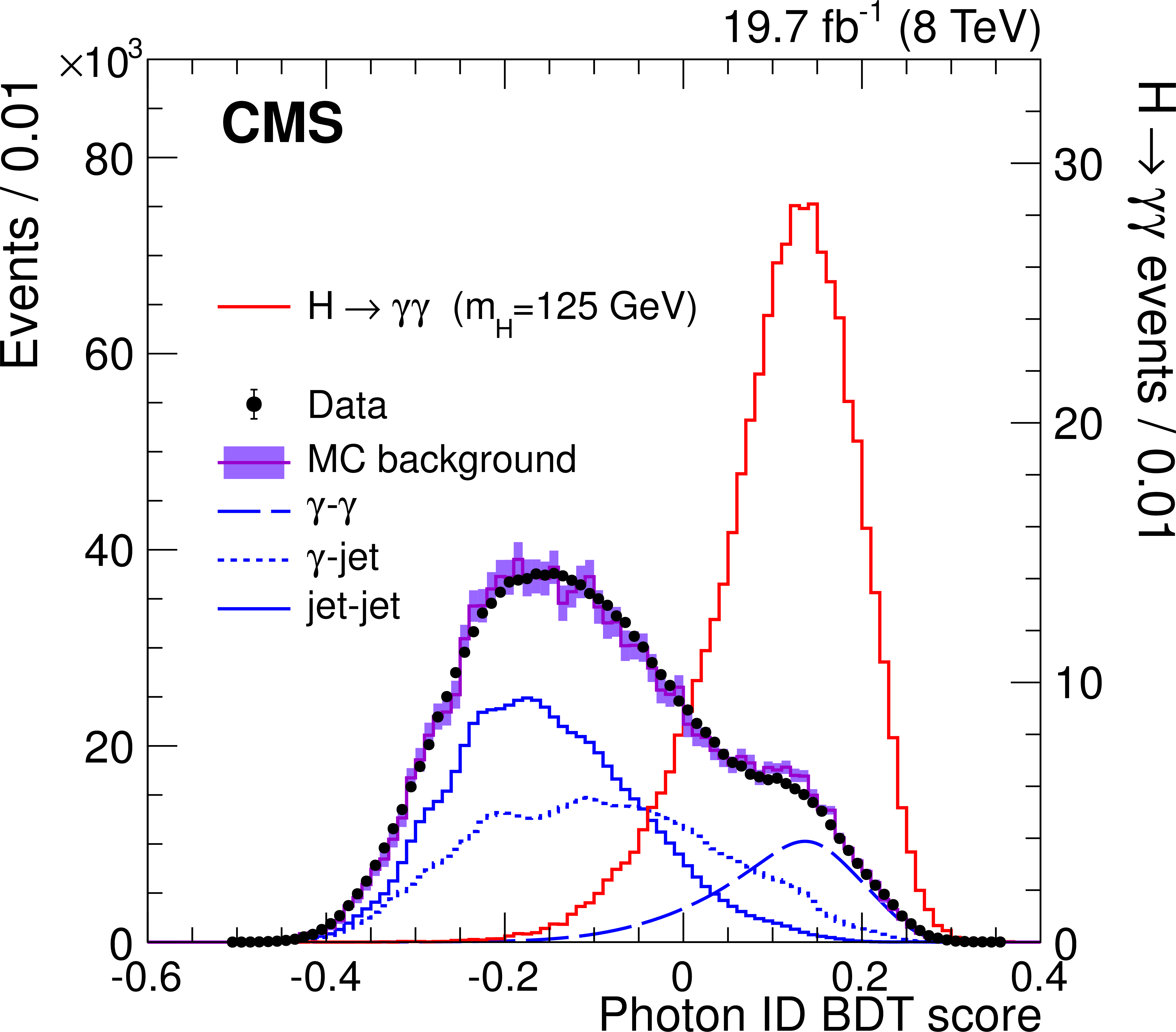
Figure 23:
Photon identification BDT score of the lower-scoring photon of the diphoton pairs with invariant masses in the range 100 $< {m_{\gamma \gamma }} <$ 180 GeV, for events passing the $ { {\mathrm {H}} \to {\gamma } {\gamma }} $ preselection in the 8 TeV dataset (points with error bars), and for simulated background events (histogram with shaded error bands showing the statistical uncertainty). The solid line histogram on the right (righthand vertical axis) is for simulated Higgs boson signal events. Histograms are also shown for different components of the simulated background, in which there are either two, one, or zero prompt signal-like photons. |
png pdf |
Figure 24-a:
Selection efficiency, as a function of $ {p_{\mathrm {T}}} $, for a particular (example) requirement on the photon identification BDT score. The efficiency is measured with the tag-and-probe technique in $ { {\mathrm {Z}}\to {\mathrm {e}^+} {\mathrm {e}^-}} $ events where the electrons are reconstructed as photons, for photons in the (a) central barrel, $ {| \eta | } < 1$, and (b) outer endcap, $1.6 < {| \eta | } < 2$. The systematic uncertainties in the tag-and-probe efficiency measurements are shown by shaded bands. The error bars representing the statistical uncertainties are too small to be visible. |
png pdf |
Figure 24-b:
Selection efficiency, as a function of $ {p_{\mathrm {T}}} $, for a particular (example) requirement on the photon identification BDT score. The efficiency is measured with the tag-and-probe technique in $ { {\mathrm {Z}}\to {\mathrm {e}^+} {\mathrm {e}^-}} $ events where the electrons are reconstructed as photons, for photons in the (a) central barrel, $ {| \eta | } < 1$, and (b) outer endcap, $1.6 < {| \eta | } < 2$. The systematic uncertainties in the tag-and-probe efficiency measurements are shown by shaded bands. The error bars representing the statistical uncertainties are too small to be visible. |
png pdf |
Figure 25-a:
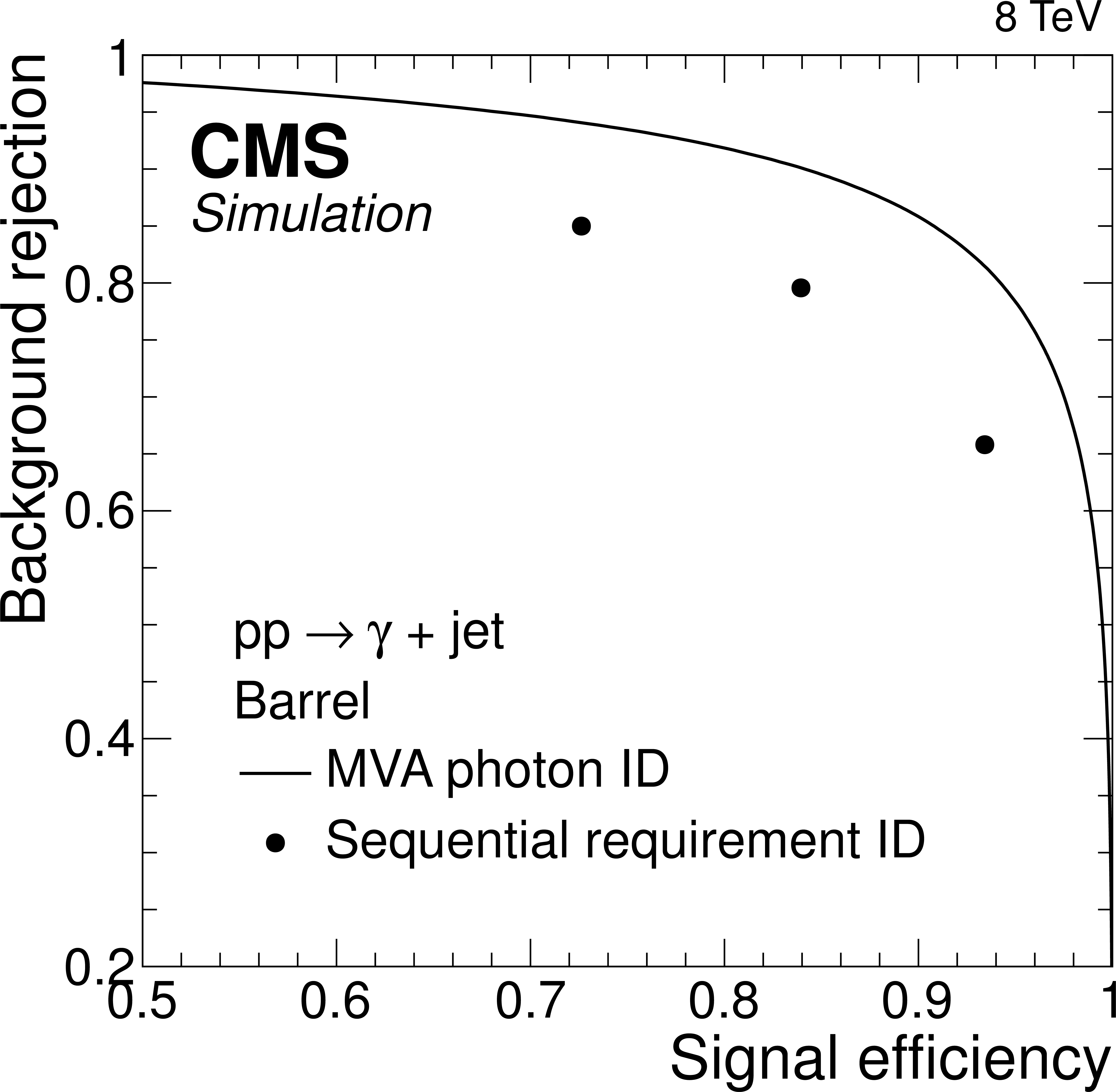
Background rejection versus signal efficiency for both sequential requirement (points) and multivariate (MVA) (curve) identification techniques in the (a) ECAL barrel and (b) endcap for simulated $ {\gamma + \text {jet}}$ events. The signal is the prompt photon and background are jets with a large electromagnetic component. A loose selection is first applied to both the simulated event samples and the values of efficiency and background rejection are relative to that (see text). |

png pdf |
Figure 25-b:
Background rejection versus signal efficiency for both sequential requirement (points) and multivariate (MVA) (curve) identification techniques in the (a) ECAL barrel and (b) endcap for simulated $ {\gamma + \text {jet}}$ events. The signal is the prompt photon and background are jets with a large electromagnetic component. A loose selection is first applied to both the simulated event samples and the values of efficiency and background rejection are relative to that (see text). |
|
|
Compact Muon Solenoid LHC, CERN |
|

|

|

|

|

|