

Compact Muon Solenoid
LHC, CERN
| CMS-EXO-12-041 ; CERN-PH-EP-2015-197 | ||
| Search for pair production of first and second generation leptoquarks in proton-proton collisions at $\sqrt{s} =$ 8 TeV | ||
| CMS Collaboration | ||
| 12 September 2015 | ||
| Phys. Rev. D93 (2016) 032004 | ||
| Abstract: A search for pair production of first and second generation leptoquarks is performed in final states containing either two charged leptons and two jets, or one charged lepton, one neutrino and two jets, using proton-proton collision data at $ \sqrt{s} = $ 8 TeV. The data, corresponding to an integrated luminosity of 19.7 fb$^{-1}$, were recorded with the CMS detector at the LHC. First-generation scalar leptoquarks with masses less than 1010 (850) GeV are excluded for $\beta =$ 1.0 (0.5), where $\beta$ is the branching fraction of a leptoquark decaying to a charged lepton and a quark. Similarly, second-generation scalar leptoquarks with masses less than 1080 (760) GeV are excluded for $\beta =$ 1.0 (0.5). Mass limits are also set for vector leptoquark production scenarios with anomalous vector couplings, and for R-parity violating supersymmetric scenarios of top squark pair production resulting in similar final-state signatures. These are the most stringent limits placed on the masses of leptoquarks and RPV top squarks to date. | ||
| Links: e-print arXiv:1509.03744 [hep-ex] (PDF) ; CDS record ; inSPIRE record ; CADI line (restricted) ; | ||
| Figures | |
png pdf |
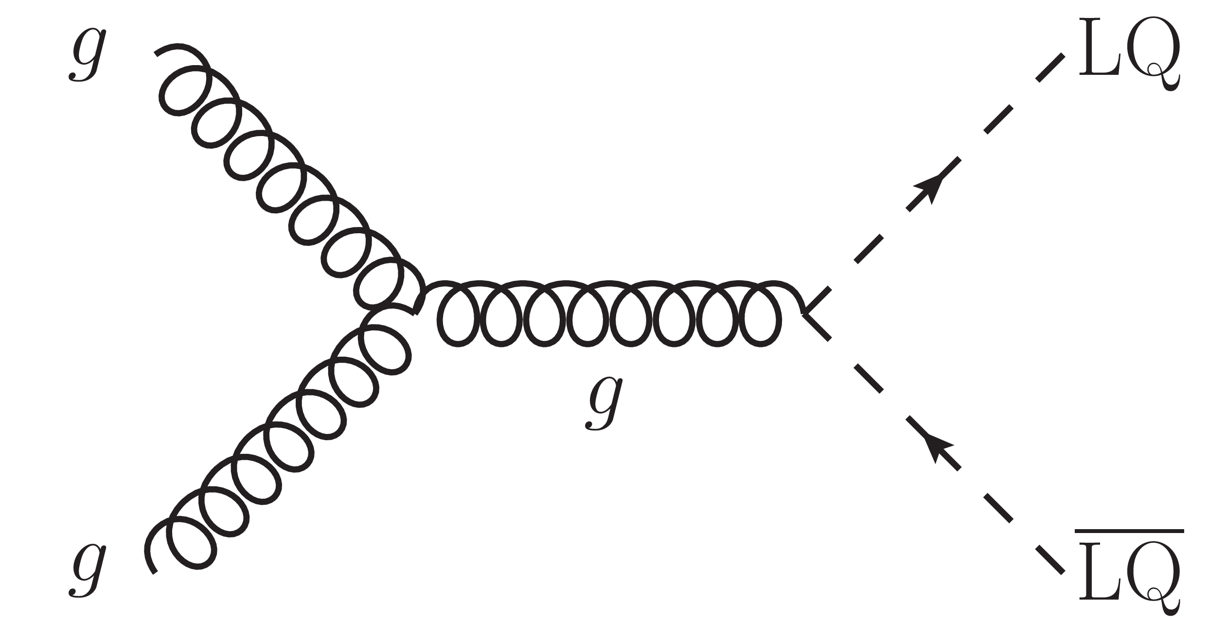
Figure 1-a:
Dominant leading order diagrams for the pair production of scalar leptoquarks. |
png pdf |
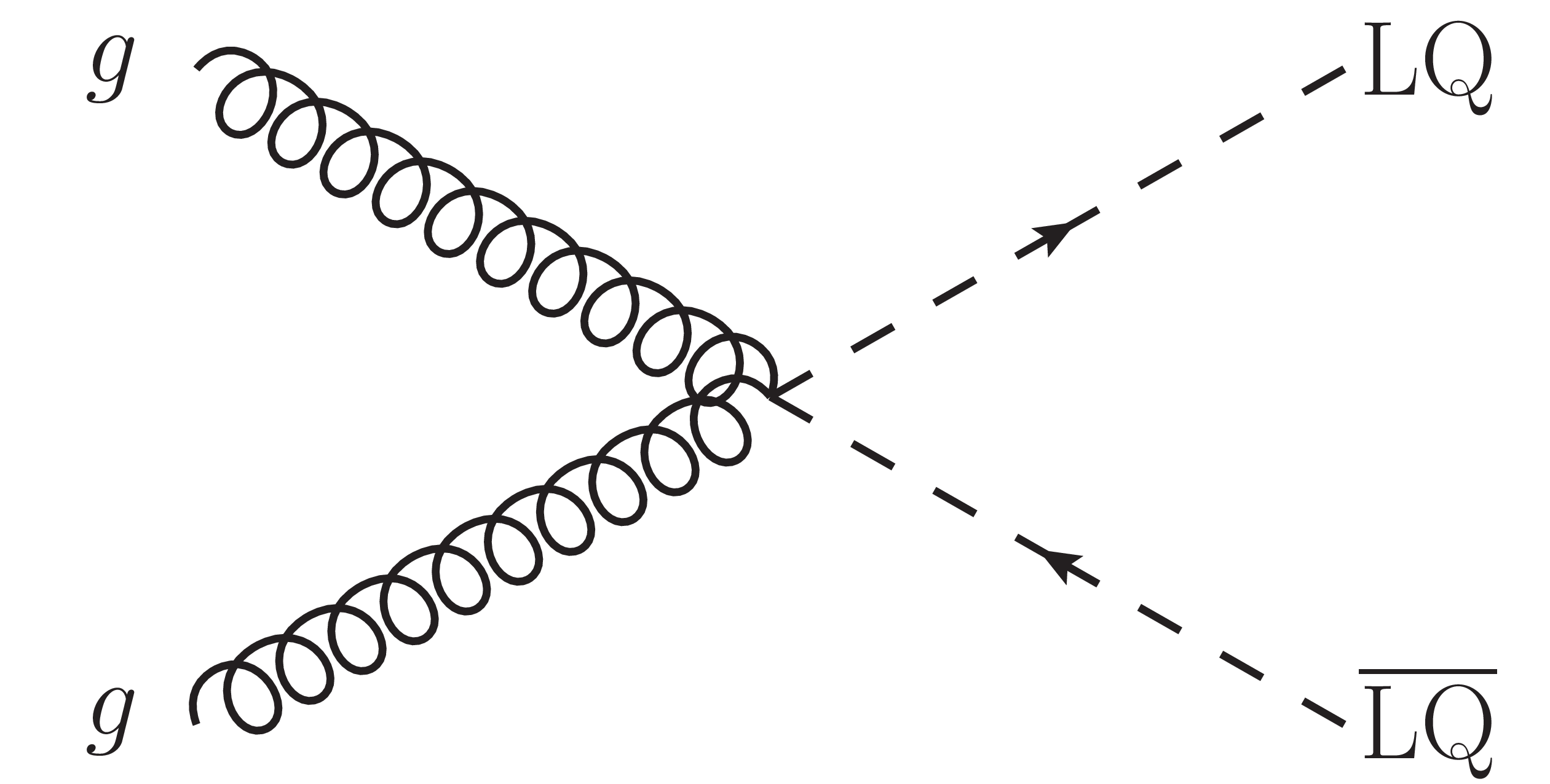
Figure 1-b:
Dominant leading order diagrams for the pair production of scalar leptoquarks. |
png pdf |
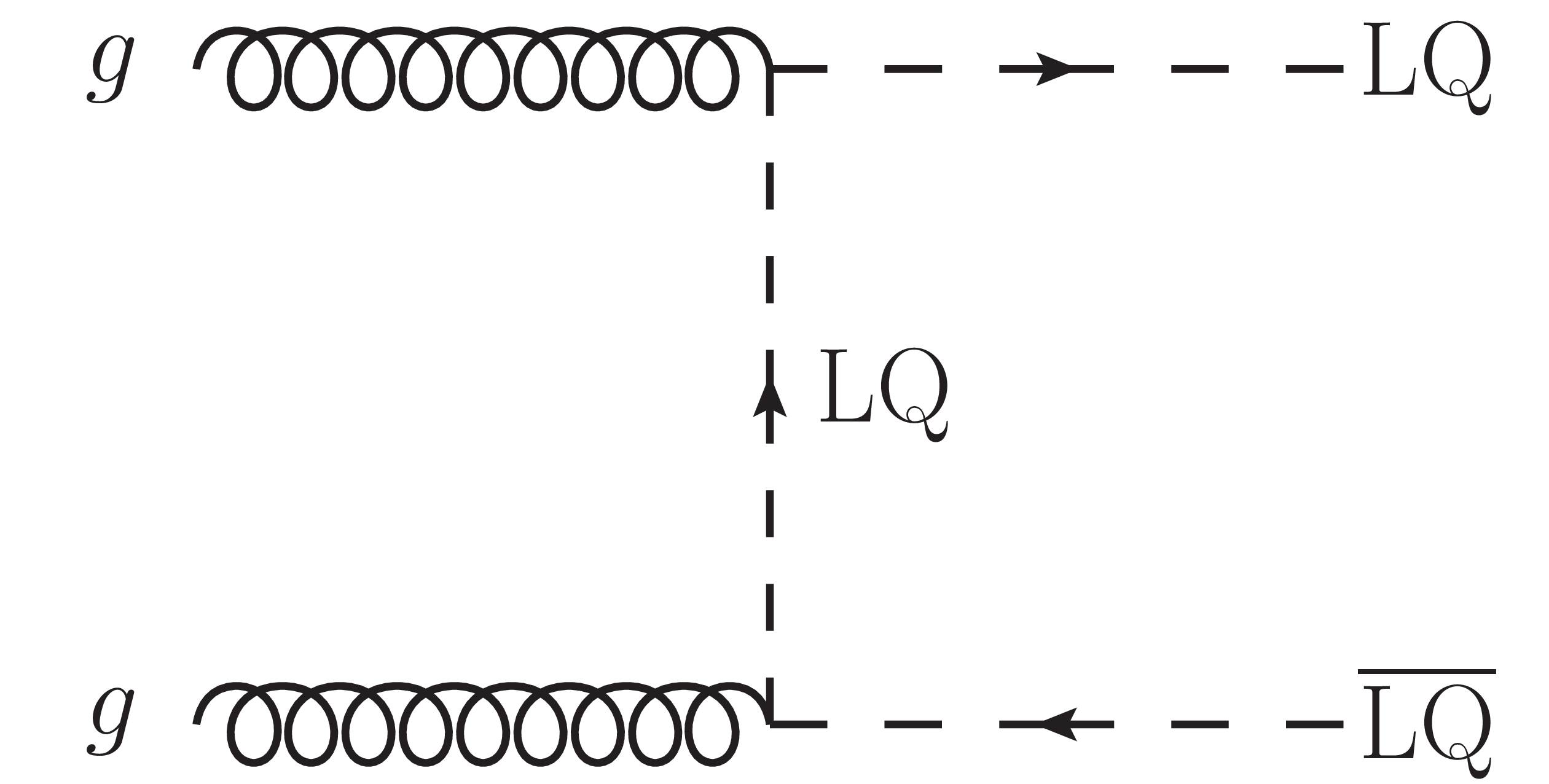
Figure 1-c:
Dominant leading order diagrams for the pair production of scalar leptoquarks. |
png pdf |
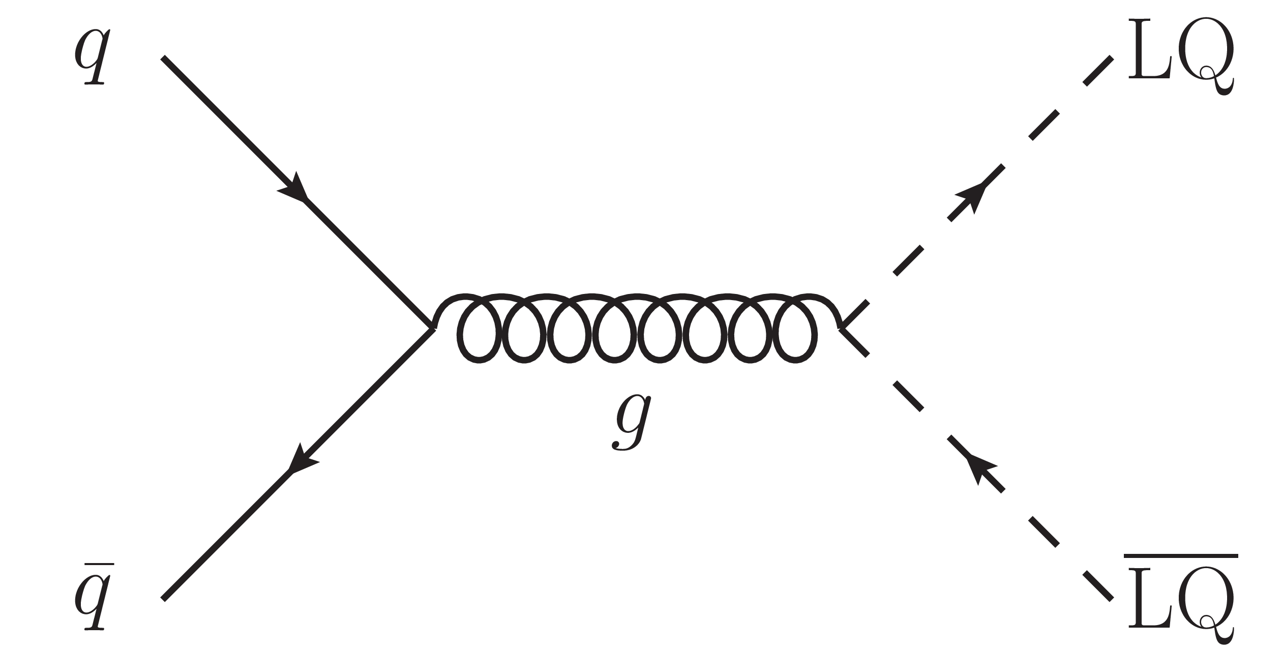
Figure 1-d:
Dominant leading order diagrams for the pair production of scalar leptoquarks. |
png pdf |
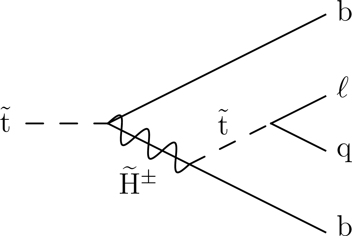
Figure 2:
Diagram of the Higgsino-mediated top squark decay via the RPV $\lambda^{\prime }_{132}$ ($\ell =$ e) or $\lambda ^{\prime }_{232}$ ($\ell = \mu $) coupling. |
png pdf |
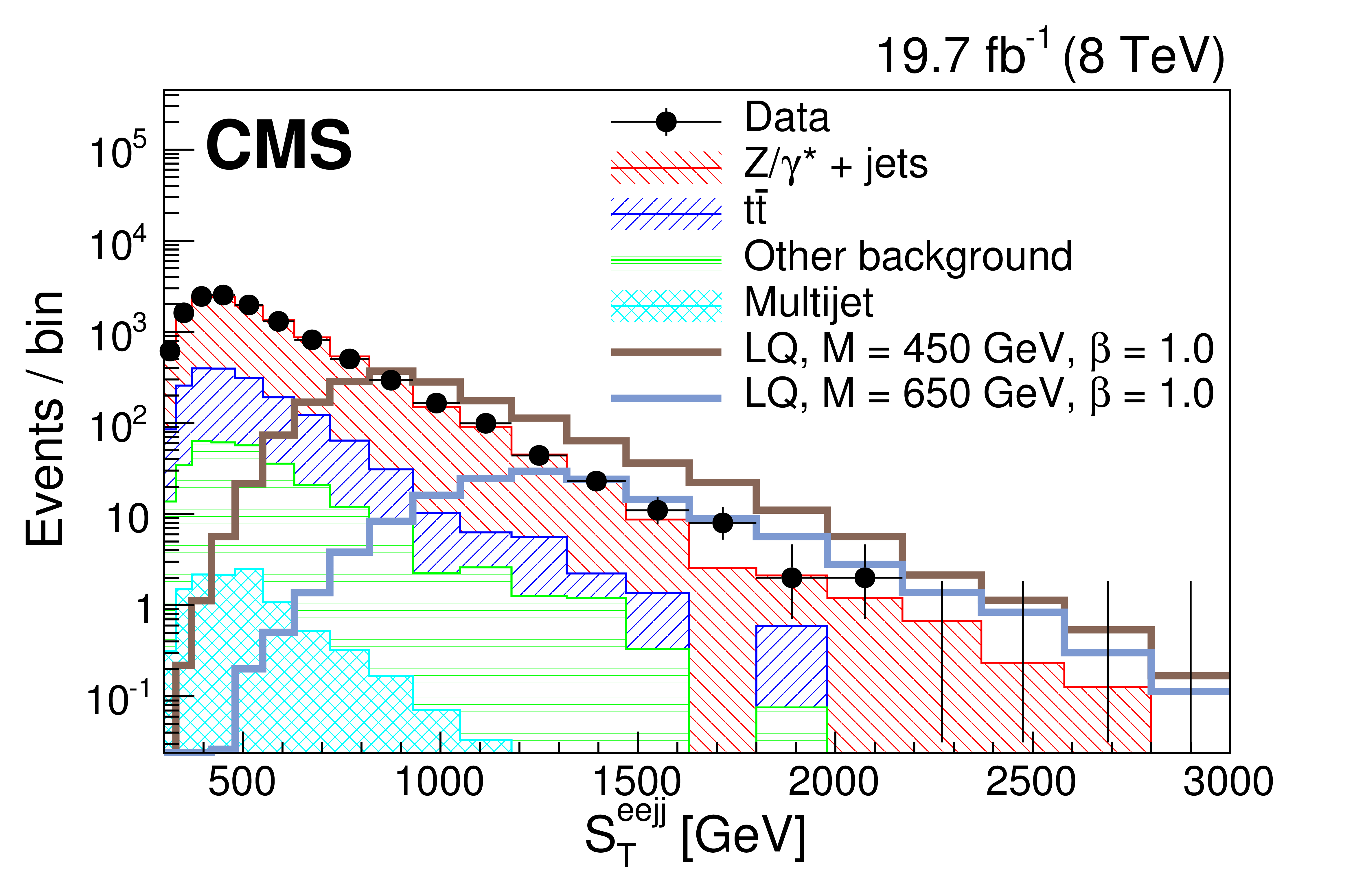
Figure 3-a:
Distributions of $S_{\mathrm {T}}$ (a,c) and $M^{\mathrm {min}}_{\ell {\mathrm {j}} }$ (b,d) at the initial selection level in the $ { {\mathrm {e}} {\mathrm {e}} {\mathrm {j}} {\mathrm {j}} } $ (a,b) and $ { {{\mu }} {{\mu }} {\mathrm {j}} {\mathrm {j}} }$ (c,d) channels. ``Other background" includes: diboson, W+jets, $\gamma $+jets, and single top quark contributions. The horizontal lines on the data points show the variable bin width. |
png pdf |
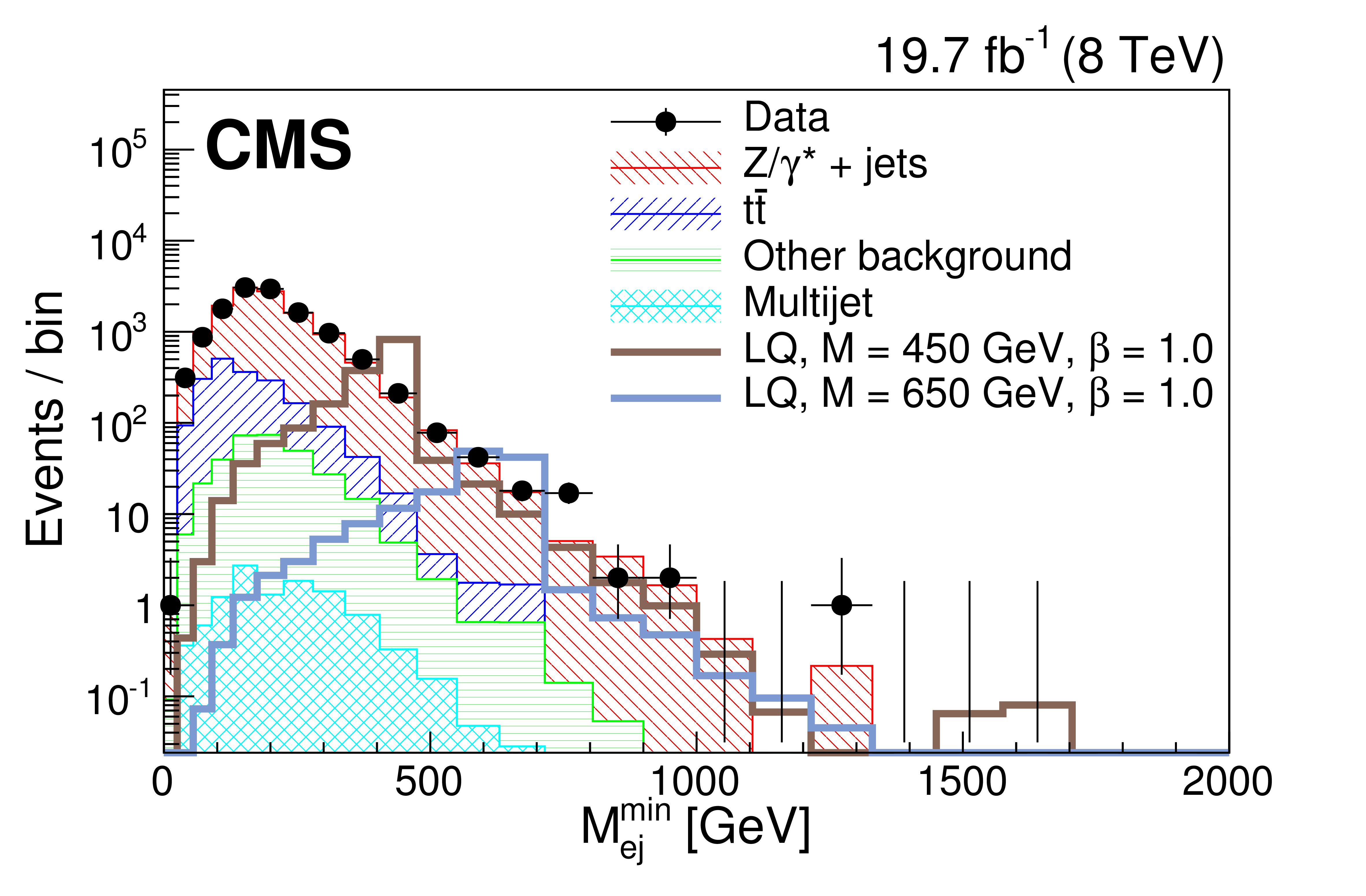
Figure 3-b:
Distributions of $S_{\mathrm {T}}$ (a,c) and $M^{\mathrm {min}}_{\ell {\mathrm {j}} }$ (b,d) at the initial selection level in the $ { {\mathrm {e}} {\mathrm {e}} {\mathrm {j}} {\mathrm {j}} } $ (a,b) and $ { {{\mu }} {{\mu }} {\mathrm {j}} {\mathrm {j}} }$ (c,d) channels. ``Other background" includes: diboson, W+jets, $\gamma $+jets, and single top quark contributions. The horizontal lines on the data points show the variable bin width. |

png pdf |
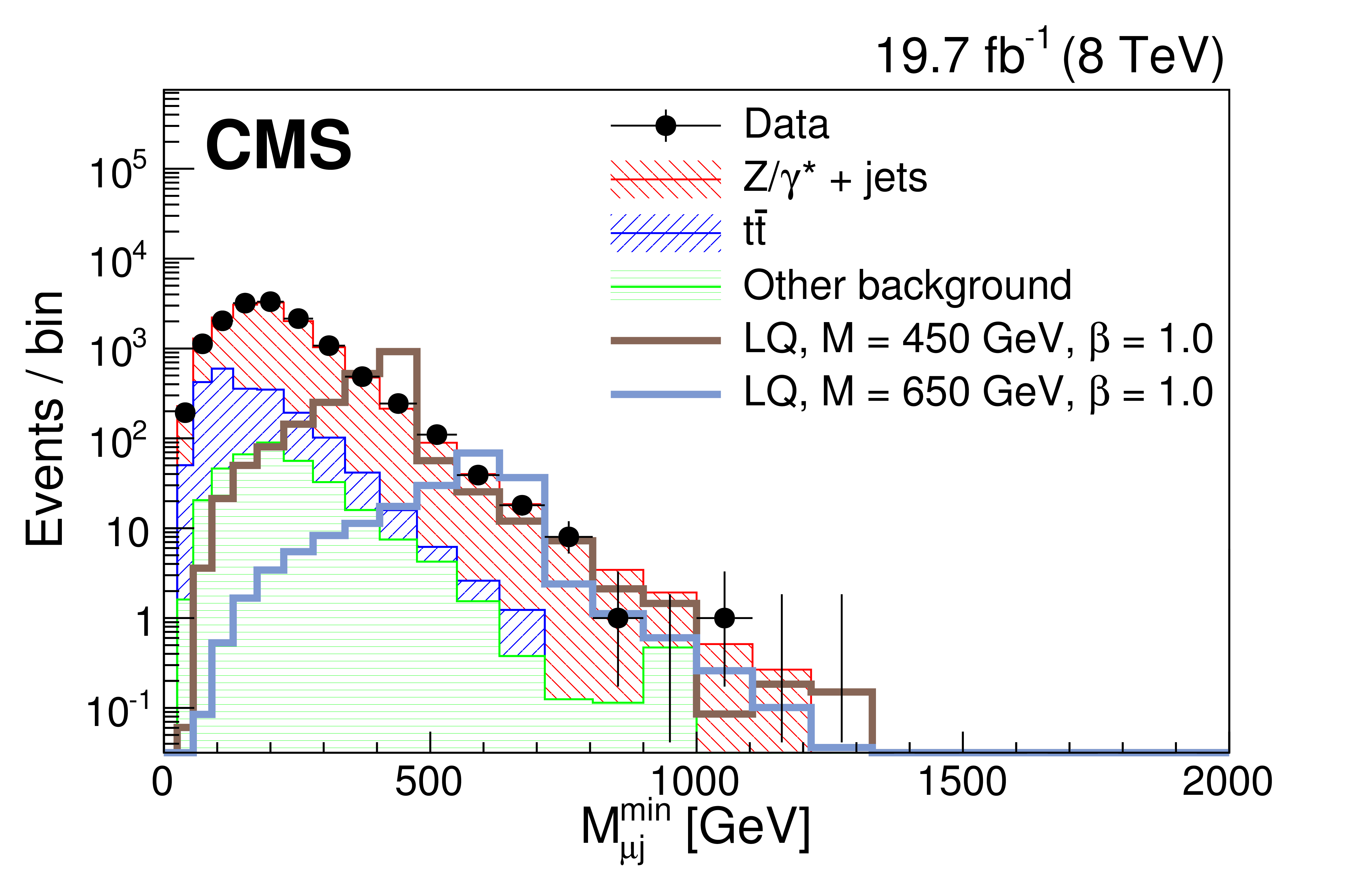
Figure 3-c:
Distributions of $S_{\mathrm {T}}$ (a,c) and $M^{\mathrm {min}}_{\ell {\mathrm {j}} }$ (b,d) at the initial selection level in the $ { {\mathrm {e}} {\mathrm {e}} {\mathrm {j}} {\mathrm {j}} } $ (a,b) and $ { {{\mu }} {{\mu }} {\mathrm {j}} {\mathrm {j}} }$ (c,d) channels. ``Other background" includes: diboson, W+jets, $\gamma $+jets, and single top quark contributions. The horizontal lines on the data points show the variable bin width. |
png pdf |
Figure 3-d:
Distributions of $S_{\mathrm {T}}$ (a,c) and $M^{\mathrm {min}}_{\ell {\mathrm {j}} }$ (b,d) at the initial selection level in the $ { {\mathrm {e}} {\mathrm {e}} {\mathrm {j}} {\mathrm {j}} } $ (a,b) and $ { {{\mu }} {{\mu }} {\mathrm {j}} {\mathrm {j}} }$ (c,d) channels. ``Other background" includes: diboson, W+jets, $\gamma $+jets, and single top quark contributions. The horizontal lines on the data points show the variable bin width. |
png pdf |
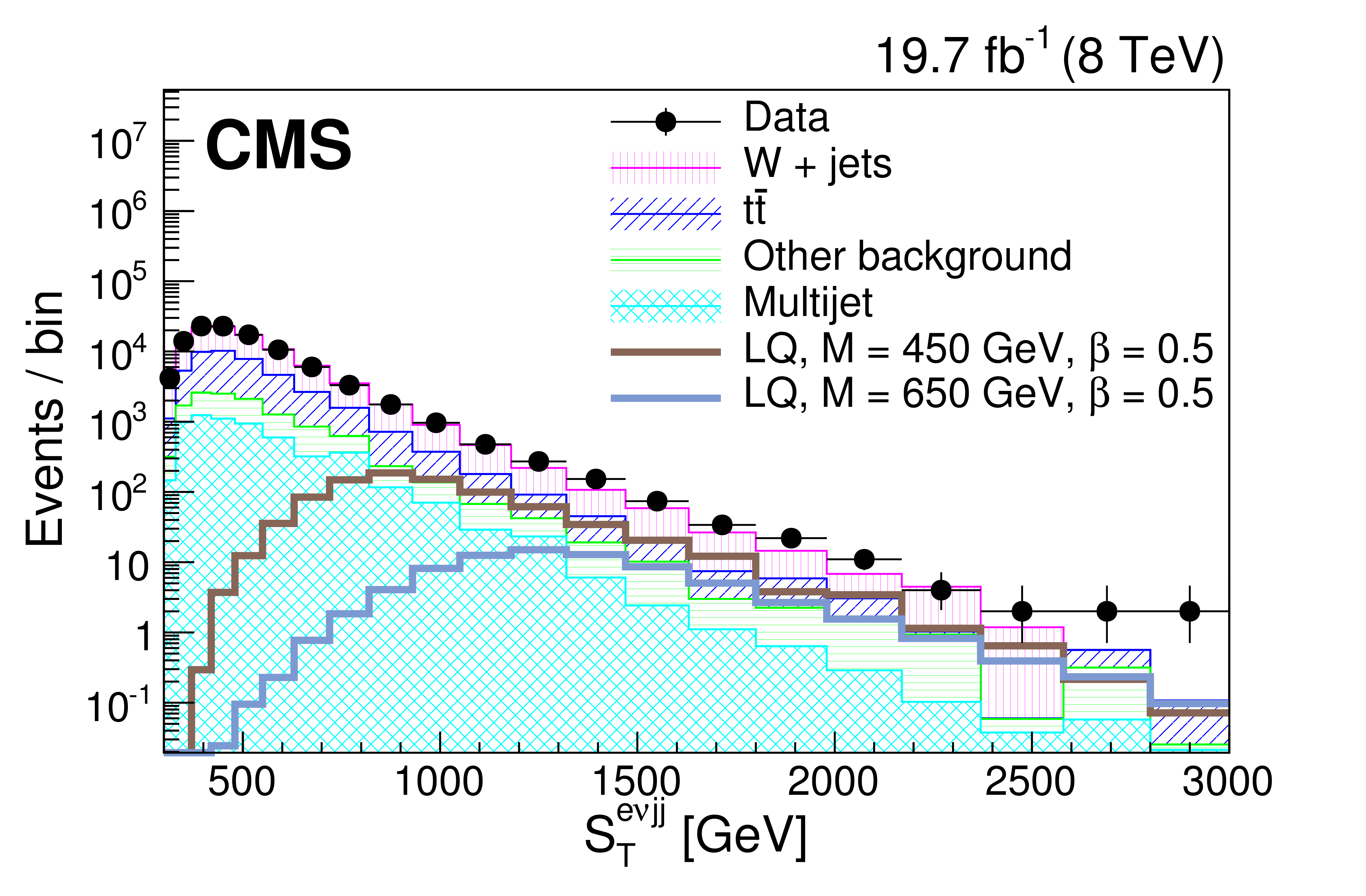
Figure 4-a:
Distributions of $S_{\mathrm {T}}$ (a,c), and $M_{\mathrm {\ell {\mathrm {j}} }}$ (b,d) at the initial selection level in the $ { {\mathrm {e}} {\nu } {\mathrm {j}} {\mathrm {j}} }$ (a,b) and $ { {{\mu }} {\nu } {\mathrm {j}} {\mathrm {j}} }$ (c,d) channels. ``Other background" includes: diboson, $ {\mathrm {Z}}/\gamma ^*$+jets, and single top quark contributions. The horizontal lines on the data points show the variable bin width. |

png pdf |
Figure 4-b:
Distributions of $S_{\mathrm {T}}$ (a,c), and $M_{\mathrm {\ell {\mathrm {j}} }}$ (b,d) at the initial selection level in the $ { {\mathrm {e}} {\nu } {\mathrm {j}} {\mathrm {j}} }$ (a,b) and $ { {{\mu }} {\nu } {\mathrm {j}} {\mathrm {j}} }$ (c,d) channels. ``Other background" includes: diboson, $ {\mathrm {Z}}/\gamma ^*$+jets, and single top quark contributions. The horizontal lines on the data points show the variable bin width. |
png pdf |
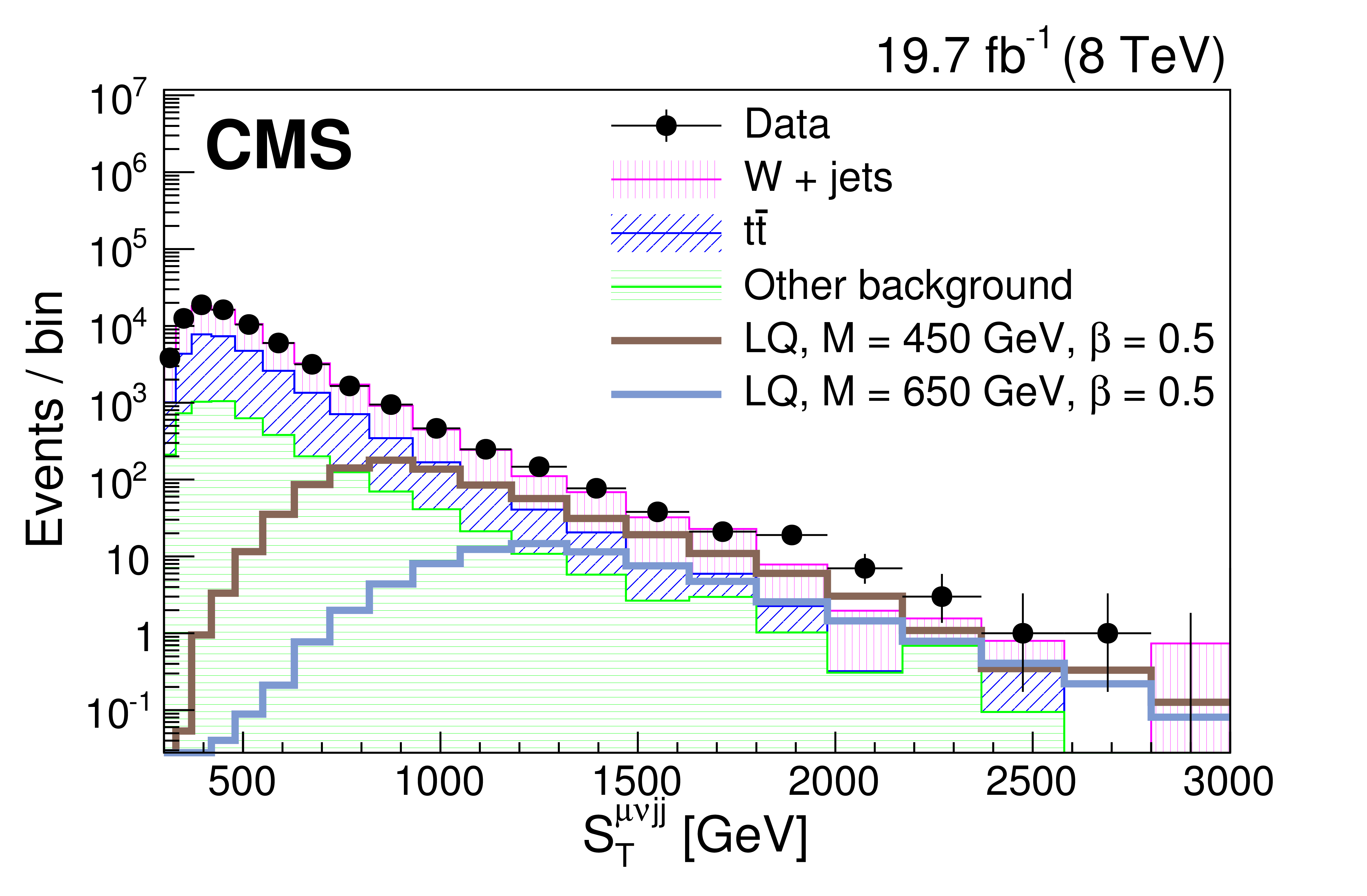
Figure 4-c:
Distributions of $S_{\mathrm {T}}$ (a,c), and $M_{\mathrm {\ell {\mathrm {j}} }}$ (b,d) at the initial selection level in the $ { {\mathrm {e}} {\nu } {\mathrm {j}} {\mathrm {j}} }$ (a,b) and $ { {{\mu }} {\nu } {\mathrm {j}} {\mathrm {j}} }$ (c,d) channels. ``Other background" includes: diboson, $ {\mathrm {Z}}/\gamma ^*$+jets, and single top quark contributions. The horizontal lines on the data points show the variable bin width. |
png pdf |
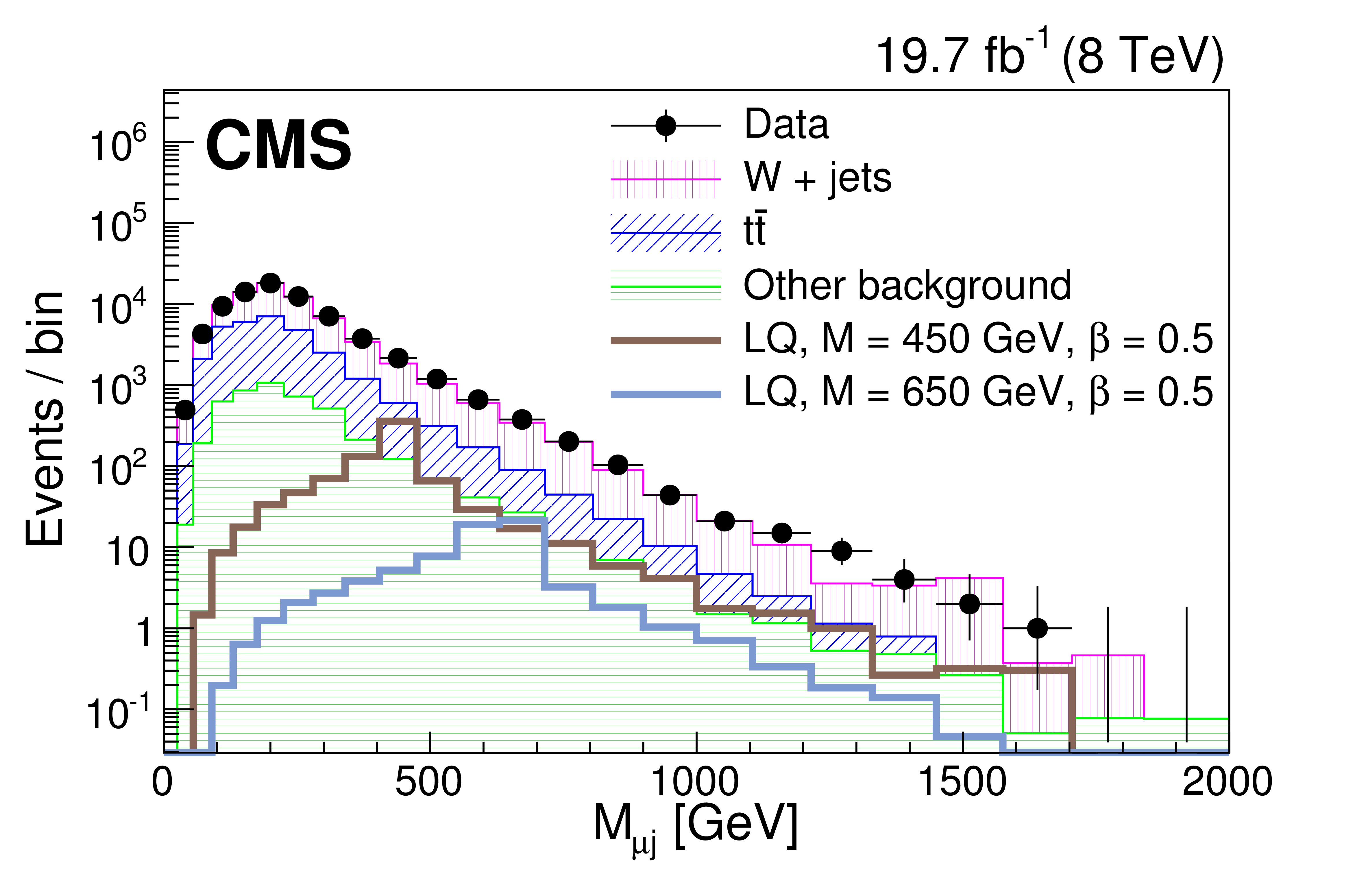
Figure 4-d:
Distributions of $S_{\mathrm {T}}$ (a,c), and $M_{\mathrm {\ell {\mathrm {j}} }}$ (b,d) at the initial selection level in the $ { {\mathrm {e}} {\nu } {\mathrm {j}} {\mathrm {j}} }$ (a,b) and $ { {{\mu }} {\nu } {\mathrm {j}} {\mathrm {j}} }$ (c,d) channels. ``Other background" includes: diboson, $ {\mathrm {Z}}/\gamma ^*$+jets, and single top quark contributions. The horizontal lines on the data points show the variable bin width. |
png pdf |
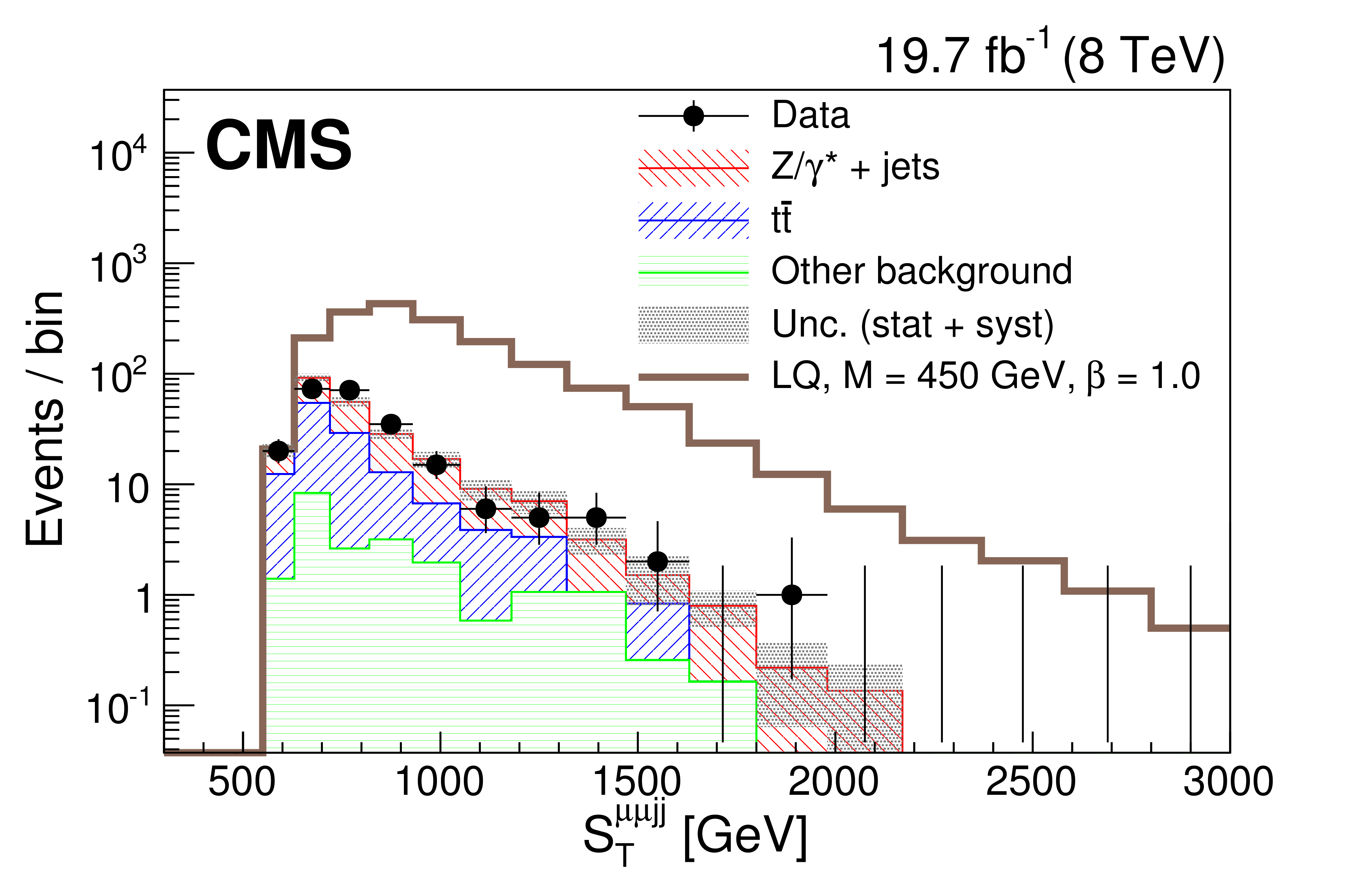
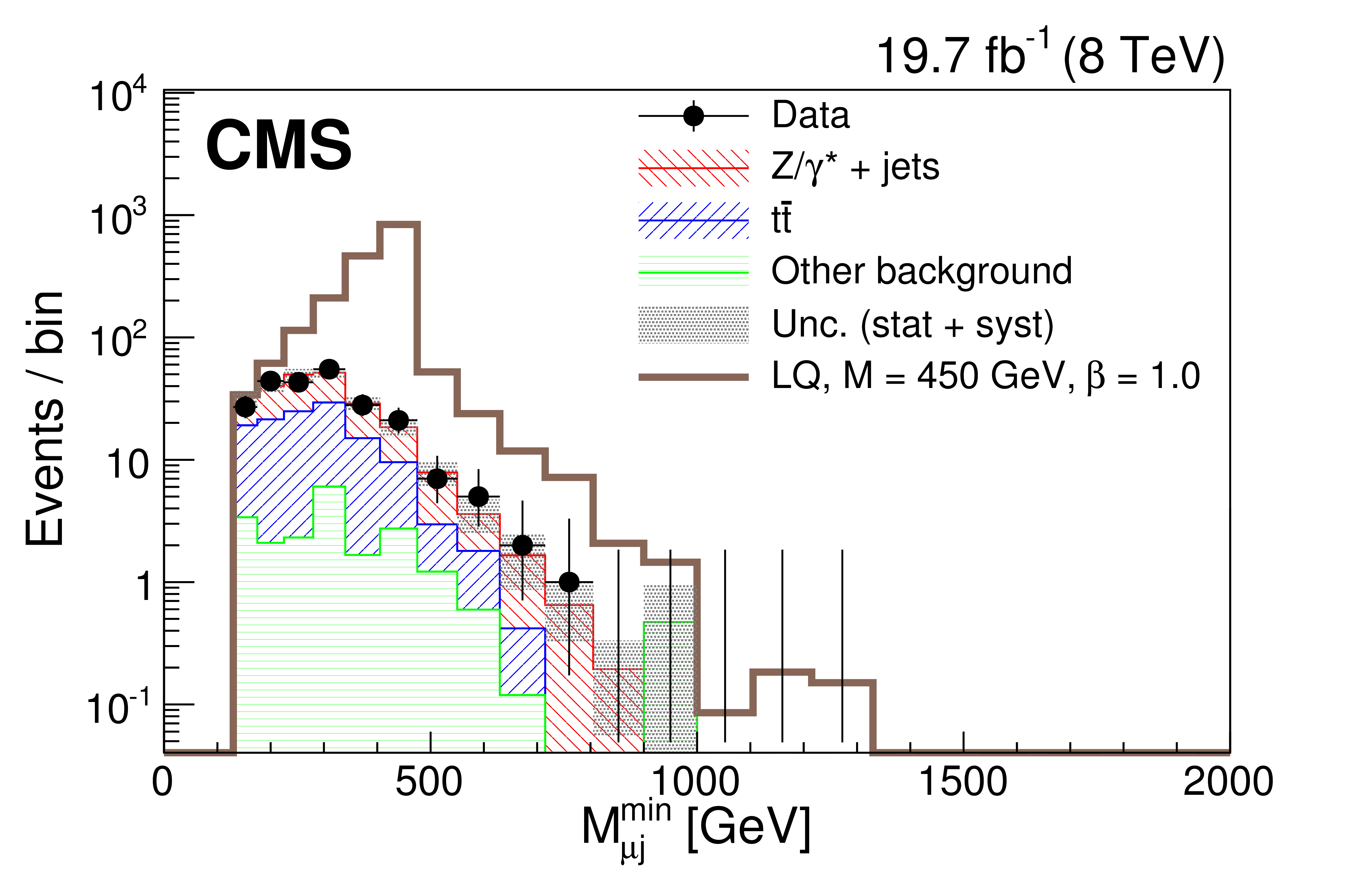
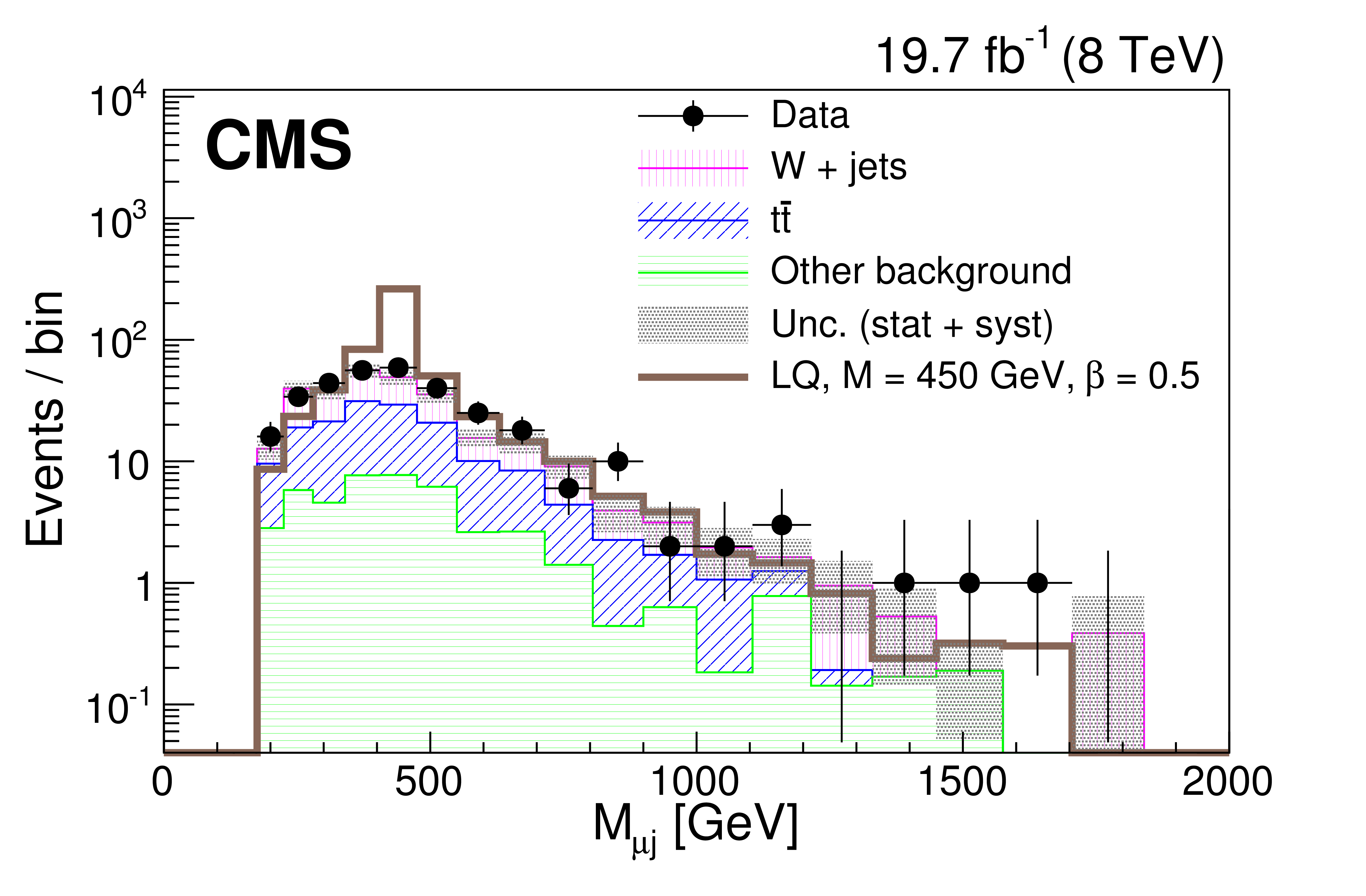
Figure 5-a:
Distributions of $S_{\mathrm {T}}$ (a,c) and $M^{\mathrm {min}}_{ {{\mu }} {\mathrm {j}} }$ (b,d) for the final selection for a LQ mass of 450 GeV (a,b) and 650 GeV (c,d) in the $ { {{\mu }} {{\mu }} {\mathrm {j}} {\mathrm {j}} }$ channel. The dark shaded region indicates the statistical and systematic uncertainty in the total background prediction. ``Other background" includes diboson, W+jets, and single top quark contributions. The horizontal lines on the data points show the variable bin width. |
png pdf |
Figure 5-b:
Distributions of $S_{\mathrm {T}}$ (a,c) and $M^{\mathrm {min}}_{ {{\mu }} {\mathrm {j}} }$ (b,d) for the final selection for a LQ mass of 450 GeV (a,b) and 650 GeV (c,d) in the $ { {{\mu }} {{\mu }} {\mathrm {j}} {\mathrm {j}} }$ channel. The dark shaded region indicates the statistical and systematic uncertainty in the total background prediction. ``Other background" includes diboson, W+jets, and single top quark contributions. The horizontal lines on the data points show the variable bin width. |
png pdf |
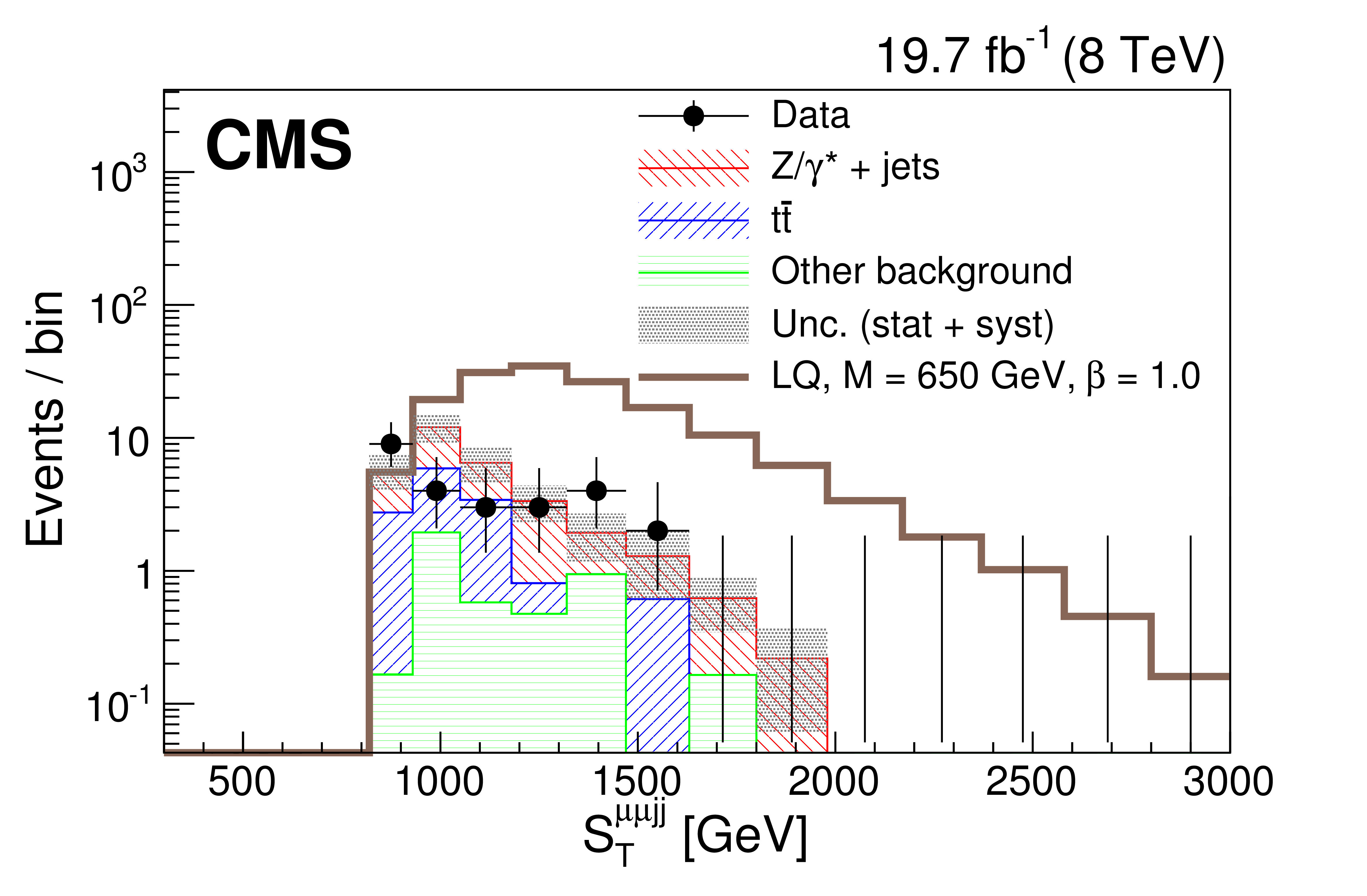
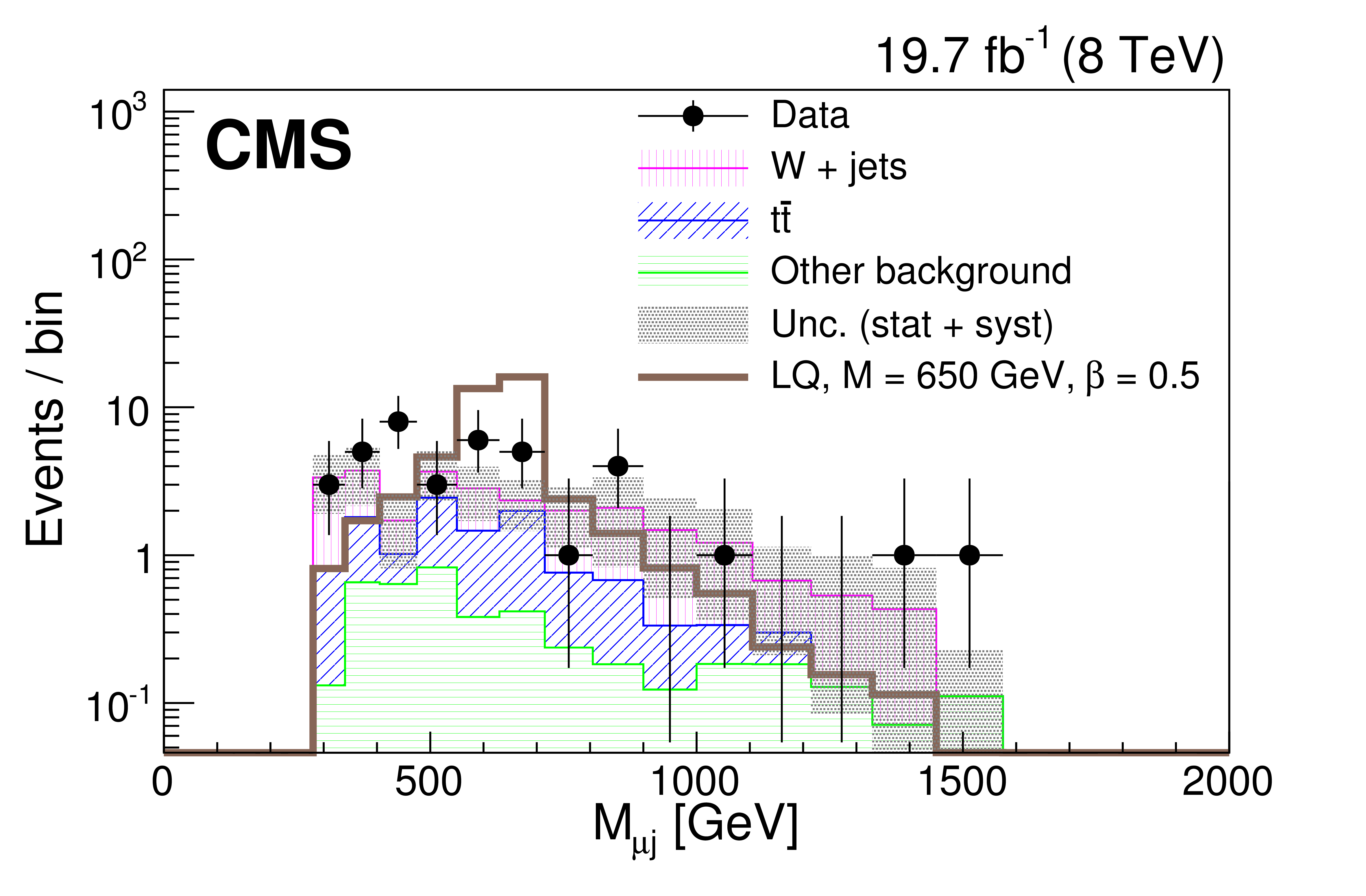
Figure 5-c:
Distributions of $S_{\mathrm {T}}$ (a,c) and $M^{\mathrm {min}}_{ {{\mu }} {\mathrm {j}} }$ (b,d) for the final selection for a LQ mass of 450 GeV (a,b) and 650 GeV (c,d) in the $ { {{\mu }} {{\mu }} {\mathrm {j}} {\mathrm {j}} }$ channel. The dark shaded region indicates the statistical and systematic uncertainty in the total background prediction. ``Other background" includes diboson, W+jets, and single top quark contributions. The horizontal lines on the data points show the variable bin width. |
png pdf |
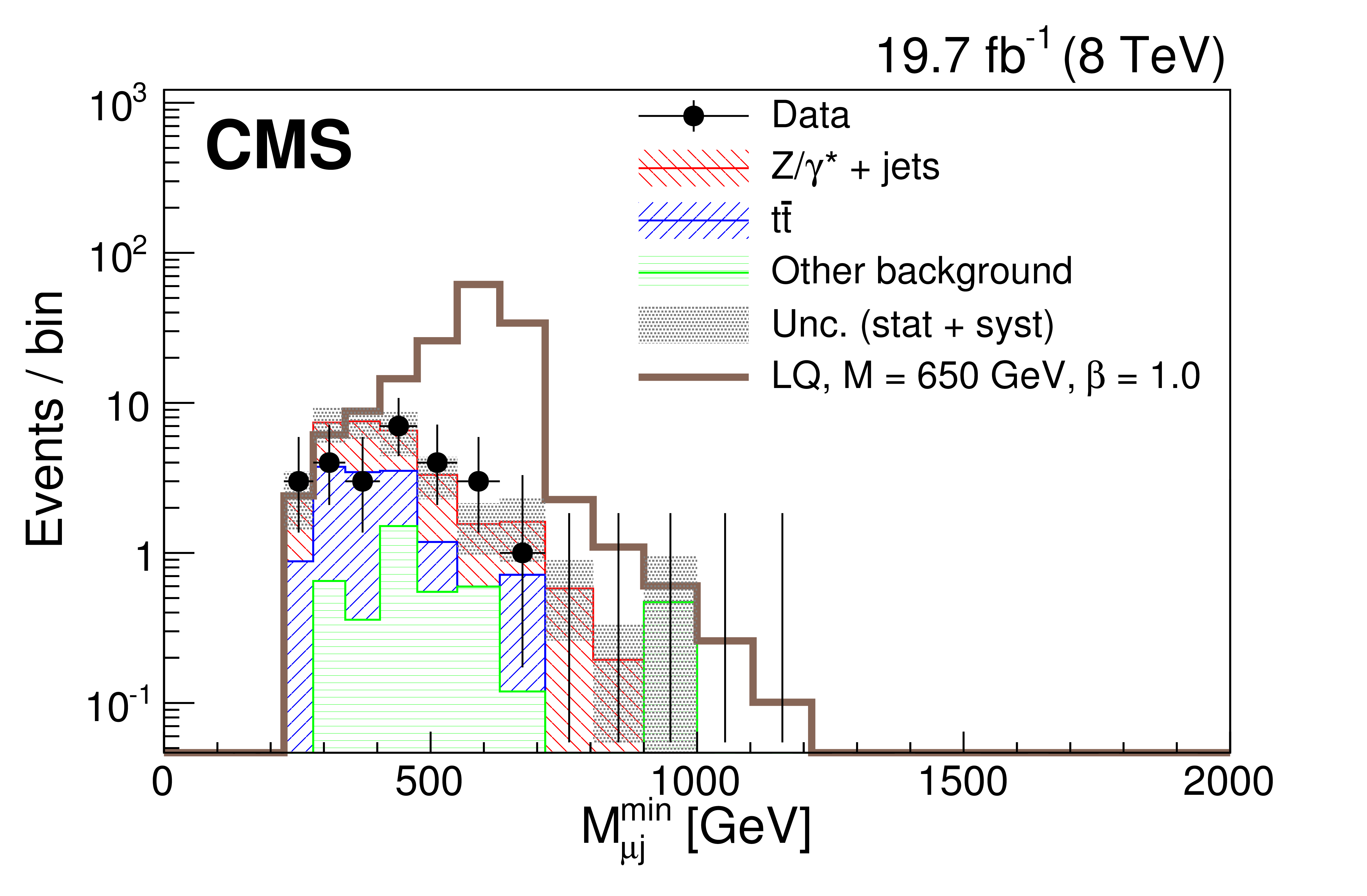
Figure 5-d:
Distributions of $S_{\mathrm {T}}$ (a,c) and $M^{\mathrm {min}}_{ {{\mu }} {\mathrm {j}} }$ (b,d) for the final selection for a LQ mass of 450 GeV (a,b) and 650 GeV (c,d) in the $ { {{\mu }} {{\mu }} {\mathrm {j}} {\mathrm {j}} }$ channel. The dark shaded region indicates the statistical and systematic uncertainty in the total background prediction. ``Other background" includes diboson, W+jets, and single top quark contributions. The horizontal lines on the data points show the variable bin width. |
png pdf |
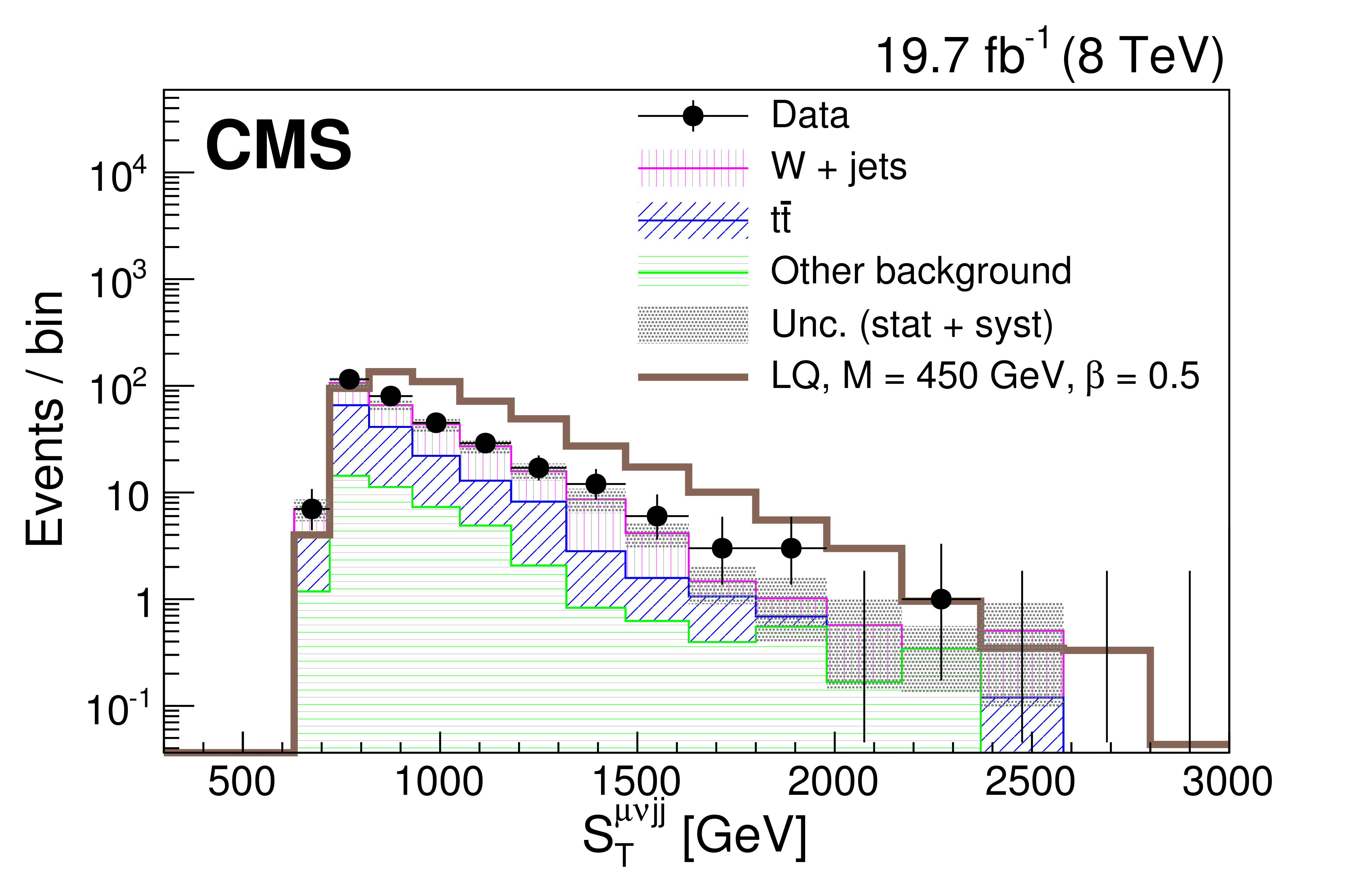
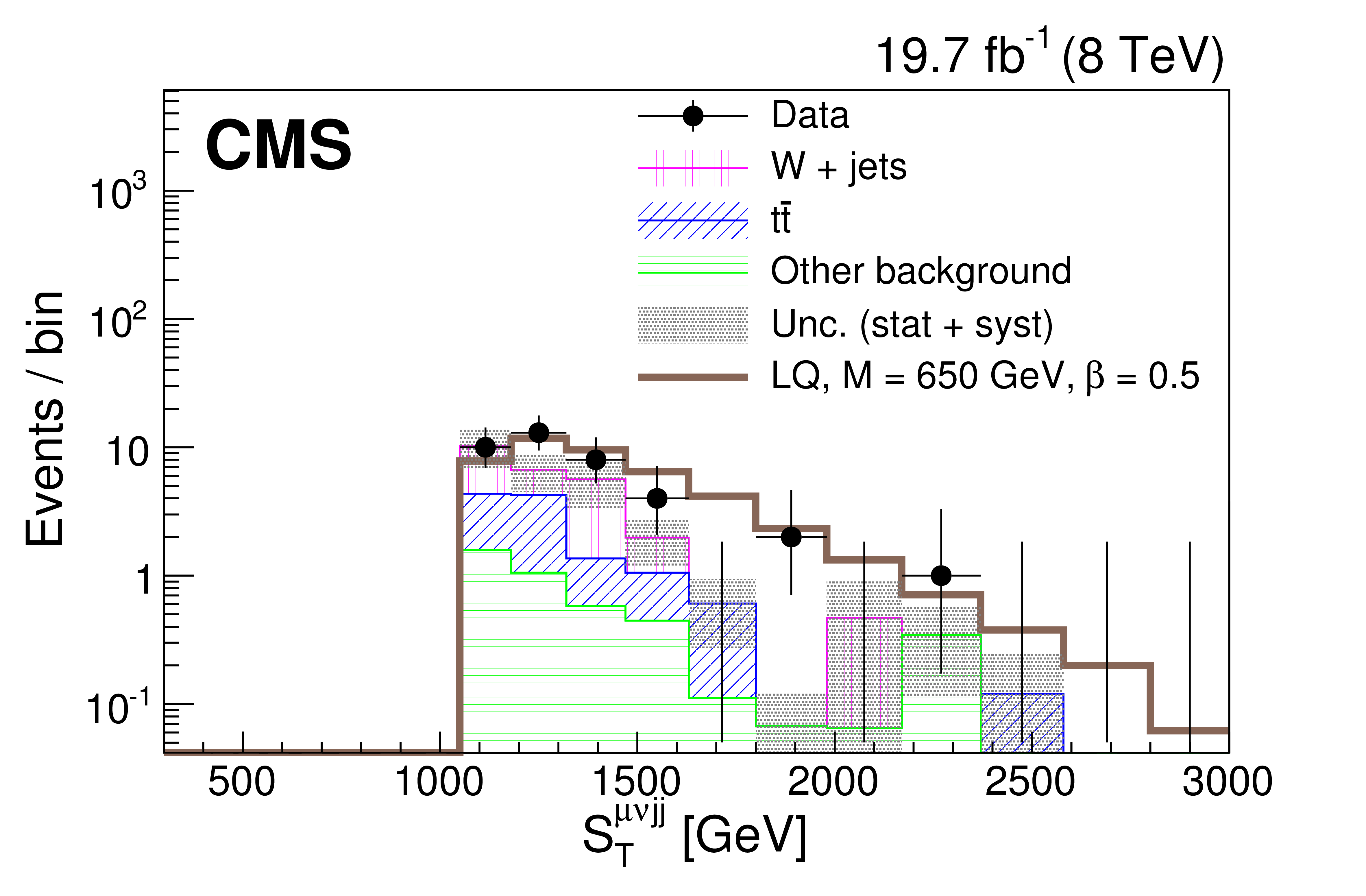
Figure 6-a:
Distributions of $S_{\mathrm {T}}$ (a,c) and $ M_{ {{\mu }} {\mathrm {j}} }$ (b,d) for the final selection for a LQ mass of 450 GeV (a,b) and 650 GeV (c,d) in the $ { {{\mu }} {\nu } {\mathrm {j}} {\mathrm {j}} }$ channel. The dark shaded region indicates the statistical and systematic uncertainty in the total background prediction. ``Other background" includes diboson, $ {\mathrm {Z}}/\gamma ^*$+jets, and single top quark contributions. The horizontal lines on the data points show the variable bin width. |
png pdf |
Figure 6-b:
Distributions of $S_{\mathrm {T}}$ (a,c) and $ M_{ {{\mu }} {\mathrm {j}} }$ (b,d) for the final selection for a LQ mass of 450 GeV (a,b) and 650 GeV (c,d) in the $ { {{\mu }} {\nu } {\mathrm {j}} {\mathrm {j}} }$ channel. The dark shaded region indicates the statistical and systematic uncertainty in the total background prediction. ``Other background" includes diboson, $ {\mathrm {Z}}/\gamma ^*$+jets, and single top quark contributions. The horizontal lines on the data points show the variable bin width. |
png pdf |
Figure 6-c:
Distributions of $S_{\mathrm {T}}$ (a,c) and $ M_{ {{\mu }} {\mathrm {j}} }$ (b,d) for the final selection for a LQ mass of 450 GeV (a,b) and 650 GeV (c,d) in the $ { {{\mu }} {\nu } {\mathrm {j}} {\mathrm {j}} }$ channel. The dark shaded region indicates the statistical and systematic uncertainty in the total background prediction. ``Other background" includes diboson, $ {\mathrm {Z}}/\gamma ^*$+jets, and single top quark contributions. The horizontal lines on the data points show the variable bin width. |
png pdf |
Figure 6-d:
Distributions of $S_{\mathrm {T}}$ (a,c) and $ M_{ {{\mu }} {\mathrm {j}} }$ (b,d) for the final selection for a LQ mass of 450 GeV (a,b) and 650 GeV (c,d) in the $ { {{\mu }} {\nu } {\mathrm {j}} {\mathrm {j}} }$ channel. The dark shaded region indicates the statistical and systematic uncertainty in the total background prediction. ``Other background" includes diboson, $ {\mathrm {Z}}/\gamma ^*$+jets, and single top quark contributions. The horizontal lines on the data points show the variable bin width. |
png pdf |
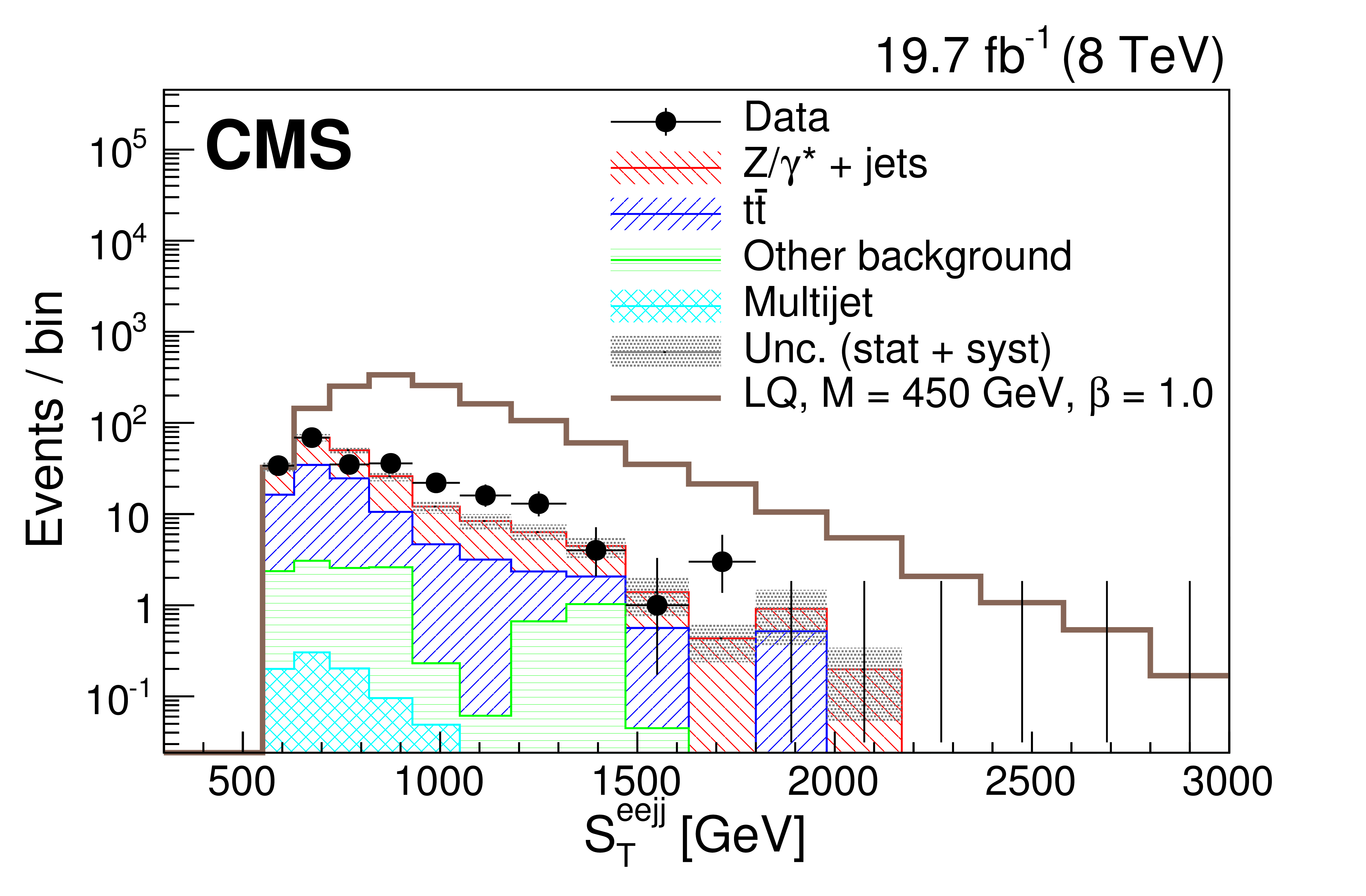
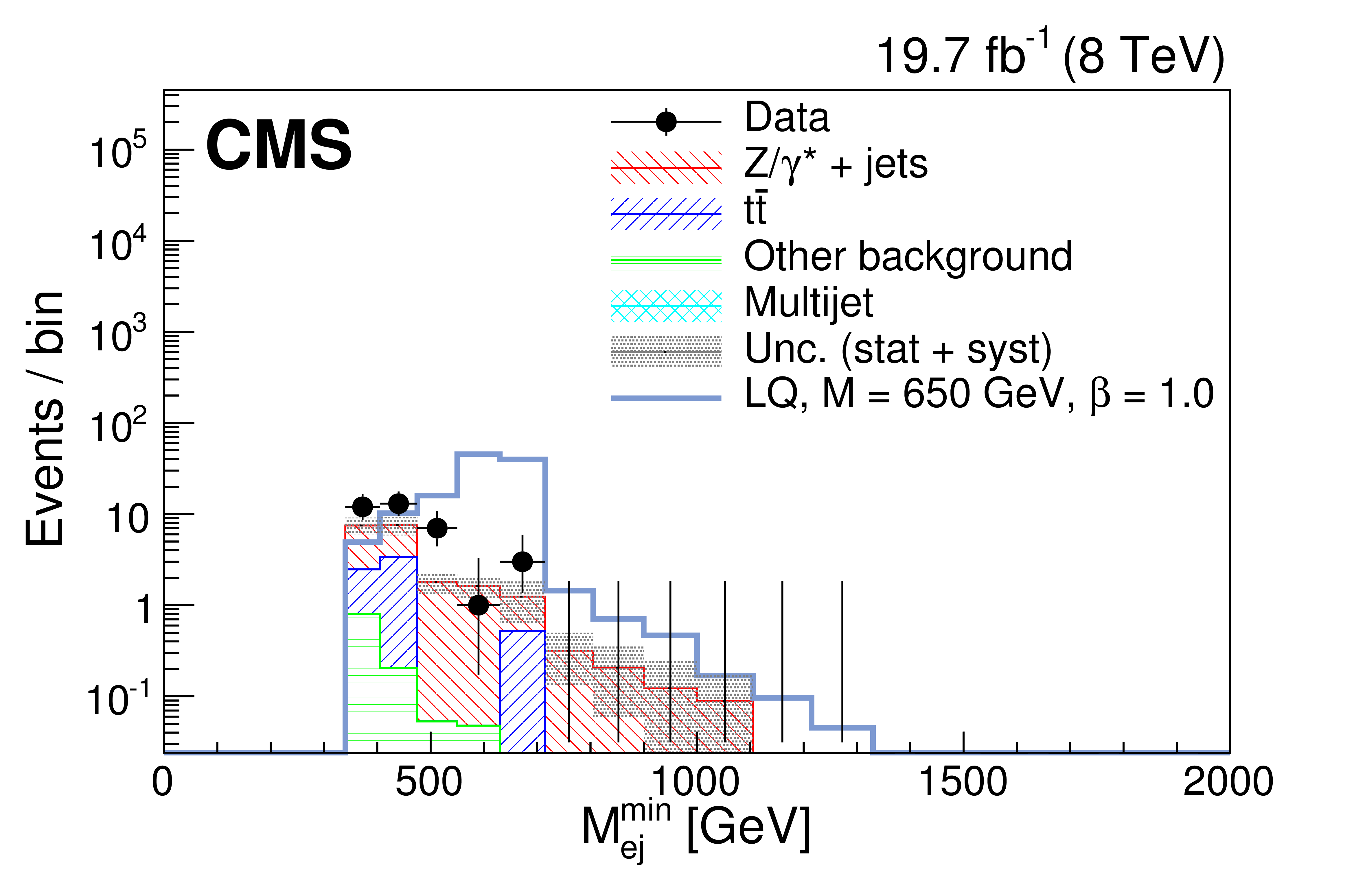
Figure 7-a:
The $S_{\mathrm {T}}$ (a,c) and $M^{\mathrm {min}}_{ {\mathrm {e}} {\mathrm {j}} }$ (b,d) distributions for events passing the $ { {\mathrm {e}} {\mathrm {e}} {\mathrm {j}} {\mathrm {j}} }$ selection optimized for $M_{\text {LQ}} = 450$ GeV (a,b) and $M_{\text {LQ}} =$ 650 GeV (c,d). The dark shaded region indicates the statistical and systematic uncertainty in the background total prediction. ``Other background" includes diboson, W+jets, and single top quark contributions. The horizontal lines on the data points show the variable bin width. |

png pdf |
Figure 7-b:
The $S_{\mathrm {T}}$ (a,c) and $M^{\mathrm {min}}_{ {\mathrm {e}} {\mathrm {j}} }$ (b,d) distributions for events passing the $ { {\mathrm {e}} {\mathrm {e}} {\mathrm {j}} {\mathrm {j}} }$ selection optimized for $M_{\text {LQ}} = 450$ GeV (a,b) and $M_{\text {LQ}} =$ 650 GeV (c,d). The dark shaded region indicates the statistical and systematic uncertainty in the background total prediction. ``Other background" includes diboson, W+jets, and single top quark contributions. The horizontal lines on the data points show the variable bin width. |

png pdf |
Figure 7-c:
The $S_{\mathrm {T}}$ (a,c) and $M^{\mathrm {min}}_{ {\mathrm {e}} {\mathrm {j}} }$ (b,d) distributions for events passing the $ { {\mathrm {e}} {\mathrm {e}} {\mathrm {j}} {\mathrm {j}} }$ selection optimized for $M_{\text {LQ}} = 450$ GeV (a,b) and $M_{\text {LQ}} =$ 650 GeV (c,d). The dark shaded region indicates the statistical and systematic uncertainty in the background total prediction. ``Other background" includes diboson, W+jets, and single top quark contributions. The horizontal lines on the data points show the variable bin width. |
png pdf |
Figure 7-d:
The $S_{\mathrm {T}}$ (a,c) and $M^{\mathrm {min}}_{ {\mathrm {e}} {\mathrm {j}} }$ (b,d) distributions for events passing the $ { {\mathrm {e}} {\mathrm {e}} {\mathrm {j}} {\mathrm {j}} }$ selection optimized for $M_{\text {LQ}} = 450$ GeV (a,b) and $M_{\text {LQ}} =$ 650 GeV (c,d). The dark shaded region indicates the statistical and systematic uncertainty in the background total prediction. ``Other background" includes diboson, W+jets, and single top quark contributions. The horizontal lines on the data points show the variable bin width. |

png pdf |
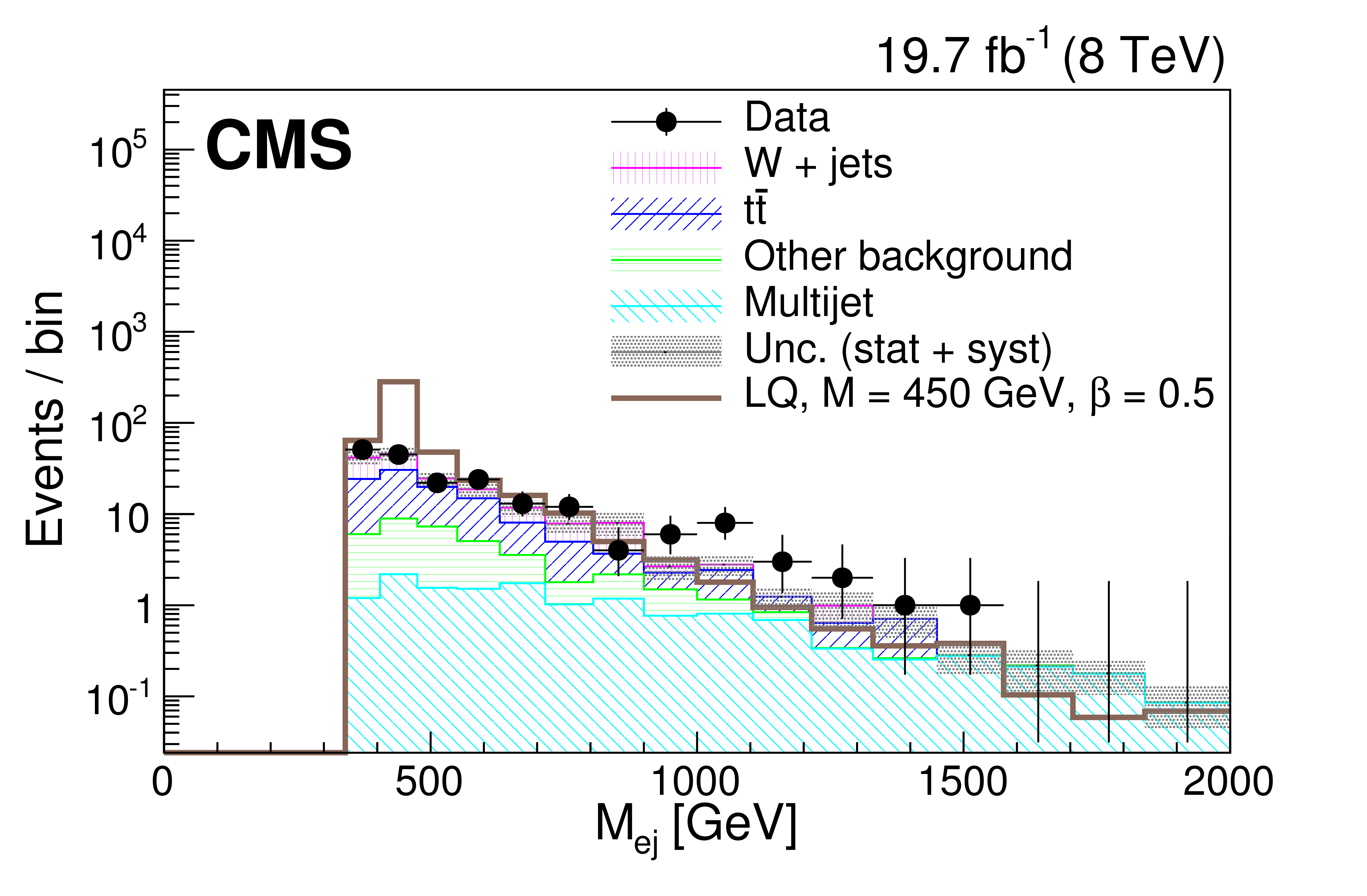
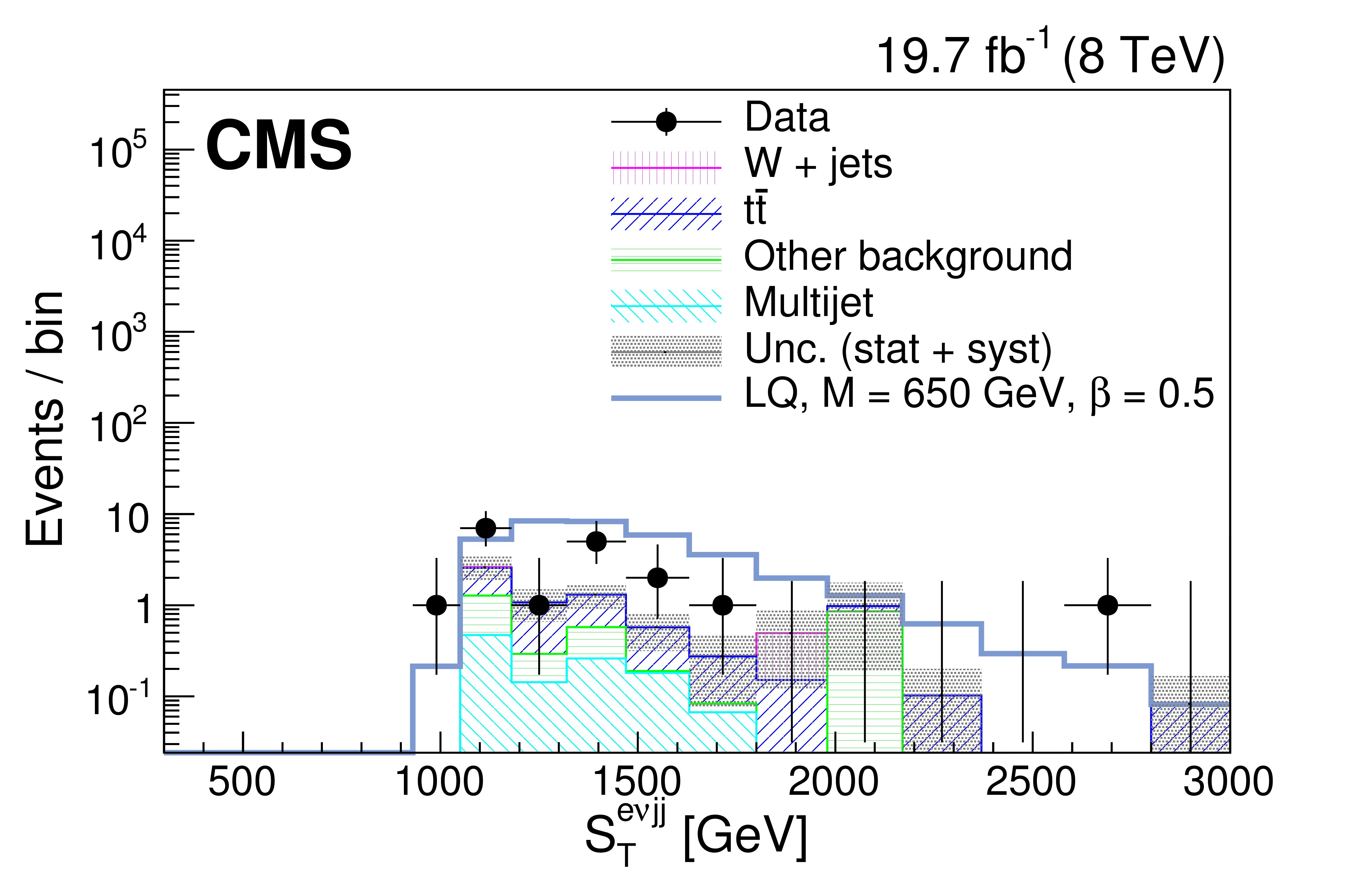
Figure 8-a:
The $S_{\mathrm {T}}$ (a,c) and $M_{ {\mathrm {e}} {\mathrm {j}} }$ (b,d) distributions for events passing the full $ { {\mathrm {e}} {\nu } {\mathrm {j}} {\mathrm {j}} }$ selection optimized for $M_{\text {LQ}} =$ 450 GeV (a,b) and $M_{\text {LQ}} =$ 650 GeV (c,d). The dark shaded region indicates the statistical and systematic uncertainty in the total background prediction. ``Other background" includes diboson, $ {\mathrm {Z}}/\gamma ^*$+jets, and single top quark contributions. The horizontal lines on the data points show the variable bin width. |
png pdf |
Figure 8-b:
The $S_{\mathrm {T}}$ (a,c) and $M_{ {\mathrm {e}} {\mathrm {j}} }$ (b,d) distributions for events passing the full $ { {\mathrm {e}} {\nu } {\mathrm {j}} {\mathrm {j}} }$ selection optimized for $M_{\text {LQ}} =$ 450 GeV (a,b) and $M_{\text {LQ}} =$ 650 GeV (c,d). The dark shaded region indicates the statistical and systematic uncertainty in the total background prediction. ``Other background" includes diboson, $ {\mathrm {Z}}/\gamma ^*$+jets, and single top quark contributions. The horizontal lines on the data points show the variable bin width. |
png pdf |
Figure 8-c:
The $S_{\mathrm {T}}$ (a,c) and $M_{ {\mathrm {e}} {\mathrm {j}} }$ (b,d) distributions for events passing the full $ { {\mathrm {e}} {\nu } {\mathrm {j}} {\mathrm {j}} }$ selection optimized for $M_{\text {LQ}} =$ 450 GeV (a,b) and $M_{\text {LQ}} =$ 650 GeV (c,d). The dark shaded region indicates the statistical and systematic uncertainty in the total background prediction. ``Other background" includes diboson, $ {\mathrm {Z}}/\gamma ^*$+jets, and single top quark contributions. The horizontal lines on the data points show the variable bin width. |
png pdf |
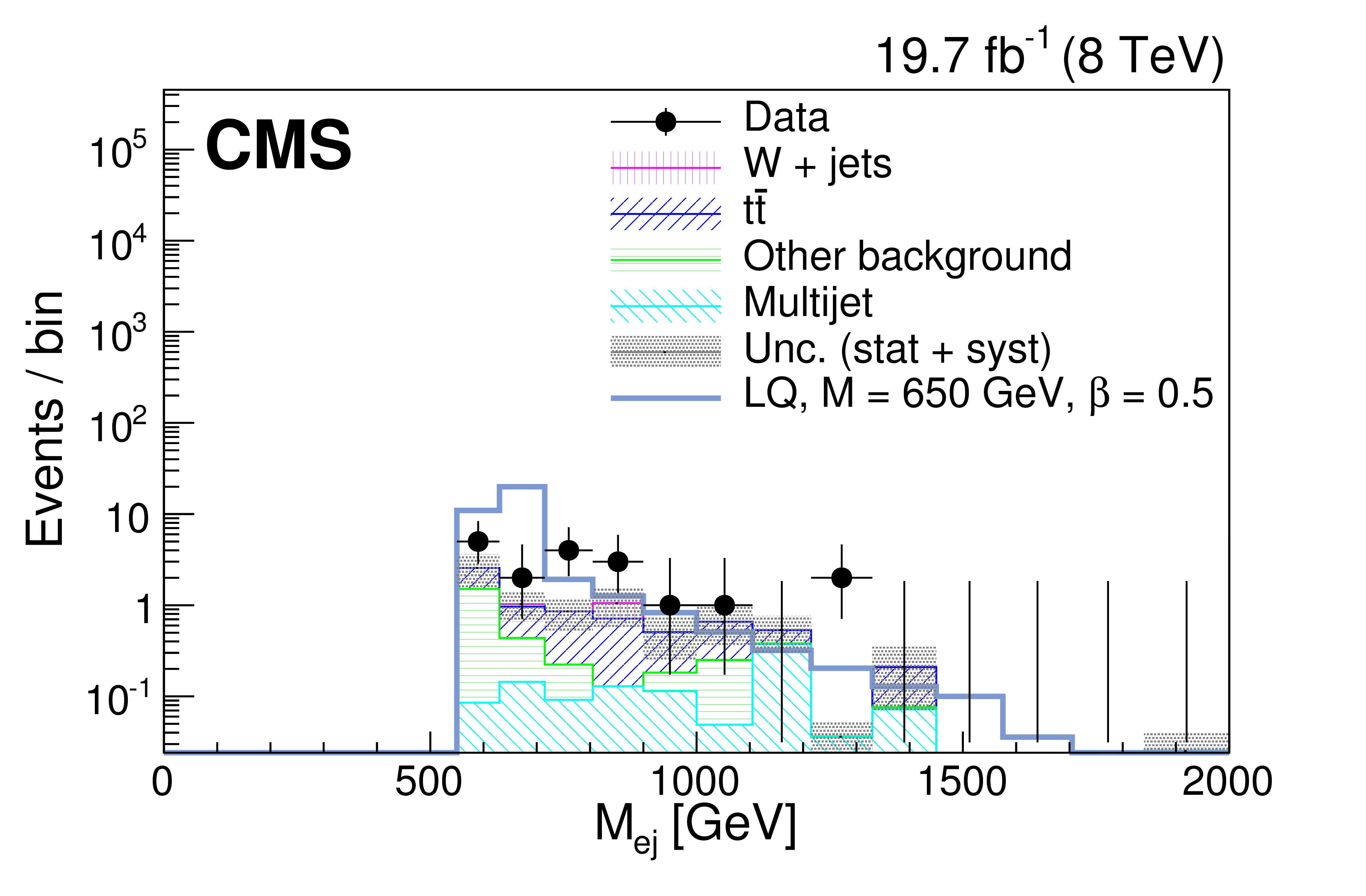
Figure 8-d:
The $S_{\mathrm {T}}$ (a,c) and $M_{ {\mathrm {e}} {\mathrm {j}} }$ (b,d) distributions for events passing the full $ { {\mathrm {e}} {\nu } {\mathrm {j}} {\mathrm {j}} }$ selection optimized for $M_{\text {LQ}} =$ 450 GeV (a,b) and $M_{\text {LQ}} =$ 650 GeV (c,d). The dark shaded region indicates the statistical and systematic uncertainty in the total background prediction. ``Other background" includes diboson, $ {\mathrm {Z}}/\gamma ^*$+jets, and single top quark contributions. The horizontal lines on the data points show the variable bin width. |
png pdf |
Figure 9-a:
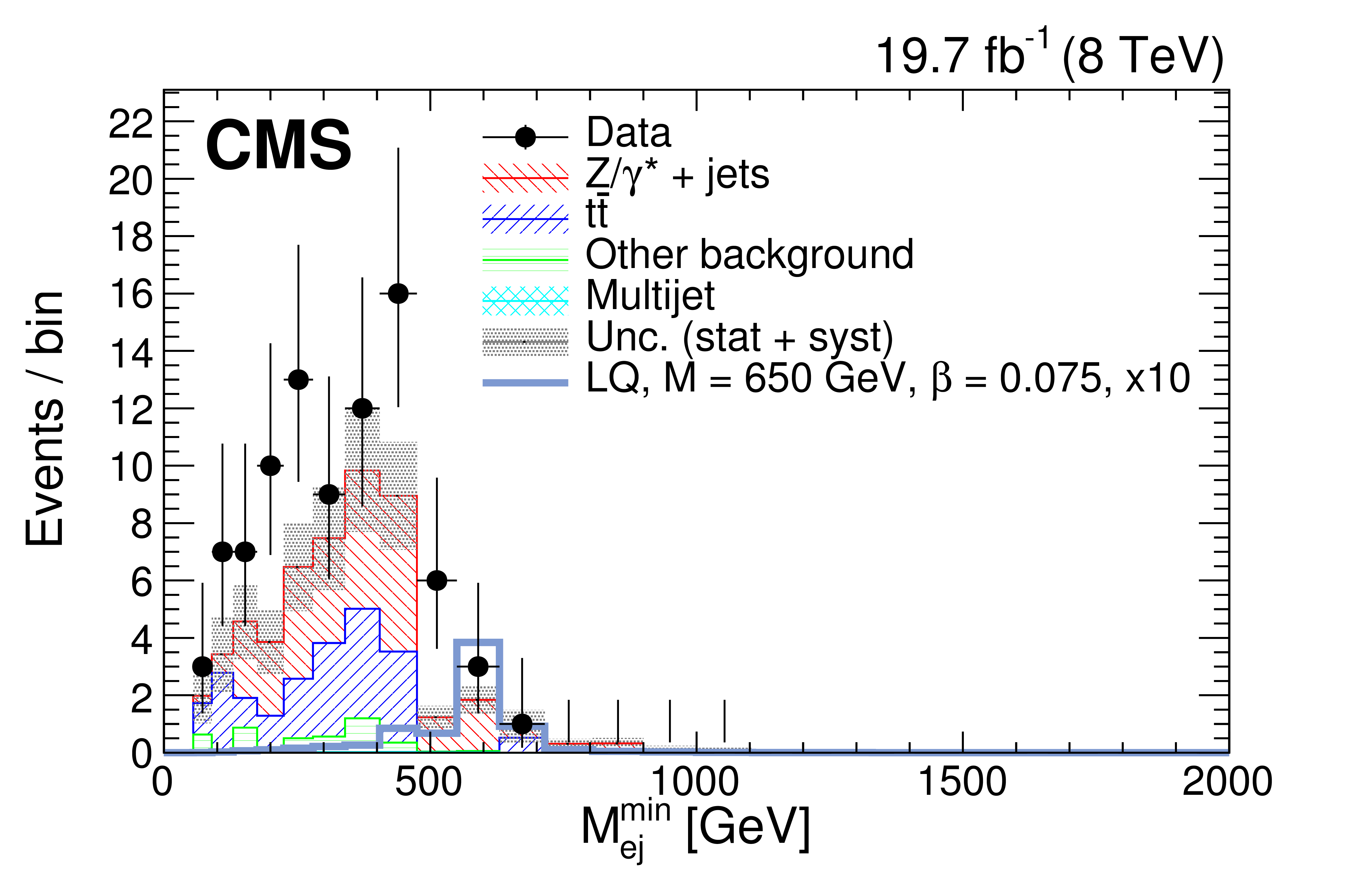
The $M^{\text {min}}_{ {\mathrm {e}} {\mathrm {j}} }$ distribution for the $ { {\mathrm {e}} {\mathrm {e}} {\mathrm {j}} {\mathrm {j}} }$ channel (a) and the $M_{ {\mathrm {e}} {\mathrm {j}} }$ distribution for the $ { {\mathrm {e}} {\nu } {\mathrm {j}} {\mathrm {j}} }$ channel (b) after the selection criteria optimized for a LQ mass of 650 GeV have been applied. The dark shaded region indicates the statistical and systematic uncertainty in the total background prediction. The signal corresponds to a LQ mass of 650 GeV and $\beta = $ 0.075. The signal is multiplied by a factor of ten in the (a) plot. In the case of the $ { {\mathrm {e}} {\mathrm {e}} {\mathrm {j}} {\mathrm {j}} }$ analysis, less than one signal event is expected to pass the selection. The horizontal lines on the data points show the variable bin width. |

png pdf |
Figure 9-b:
The $M^{\text {min}}_{ {\mathrm {e}} {\mathrm {j}} }$ distribution for the $ { {\mathrm {e}} {\mathrm {e}} {\mathrm {j}} {\mathrm {j}} }$ channel (a) and the $M_{ {\mathrm {e}} {\mathrm {j}} }$ distribution for the $ { {\mathrm {e}} {\nu } {\mathrm {j}} {\mathrm {j}} }$ channel (b) after the selection criteria optimized for a LQ mass of 650 GeV have been applied. The dark shaded region indicates the statistical and systematic uncertainty in the total background prediction. The signal corresponds to a LQ mass of 650 GeV and $\beta = $ 0.075. The signal is multiplied by a factor of ten in the (a) plot. In the case of the $ { {\mathrm {e}} {\mathrm {e}} {\mathrm {j}} {\mathrm {j}} }$ analysis, less than one signal event is expected to pass the selection. The horizontal lines on the data points show the variable bin width. |
png pdf |
Figure 10-a:
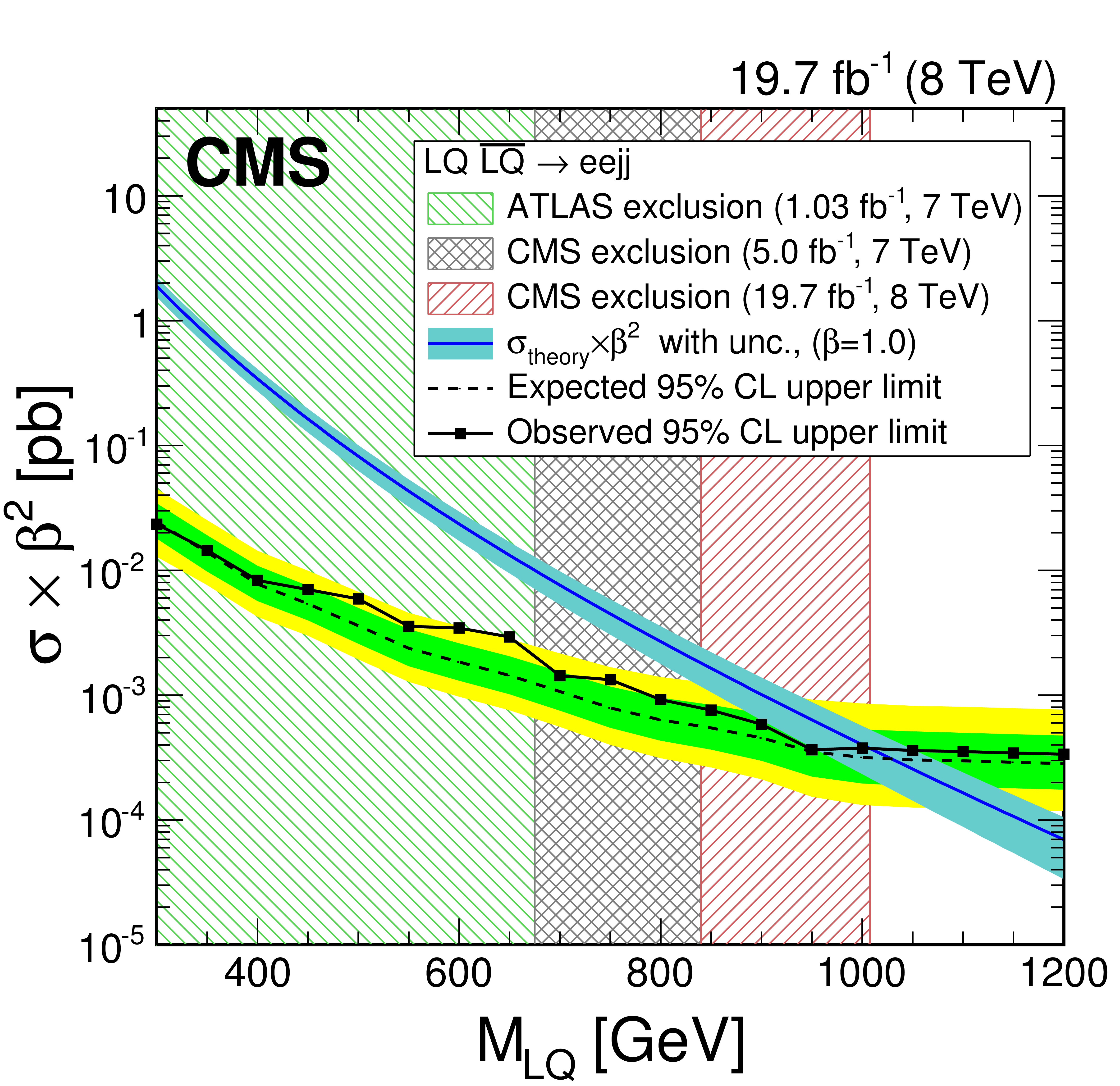
a (b): the expected and observed upper limits at 95% CL on the LQ pair production cross section times $\beta ^2$ ($2\beta (1-\beta )$) as a function of the first generation LQ mass obtained with the $ { {\mathrm {e}} {\mathrm {e}} {\mathrm {j}} {\mathrm {j}} }$ ($ { {\mathrm {e}} {\nu } {\mathrm {j}} {\mathrm {j}} }$) analysis. The expected limits and uncertainty bands represent the median expected limits and the 68% and 95% confidence intervals. The left shaded regions are excluded by Ref.[24] and the middle shaded regions are excluded by Ref.[23]. The right shaded region is excluded by the analysis presented in this paper. The $\sigma _{\rm theory}$ curves and their bands represent, respectively, the theoretical scalar LQ pair production cross section and the uncertainties due to the choice of PDF and renormalization/factorization scales. |

png pdf |
Figure 10-b:
a (b): the expected and observed upper limits at 95% CL on the LQ pair production cross section times $\beta ^2$ ($2\beta (1-\beta )$) as a function of the first generation LQ mass obtained with the $ { {\mathrm {e}} {\mathrm {e}} {\mathrm {j}} {\mathrm {j}} }$ ($ { {\mathrm {e}} {\nu } {\mathrm {j}} {\mathrm {j}} }$) analysis. The expected limits and uncertainty bands represent the median expected limits and the 68% and 95% confidence intervals. The left shaded regions are excluded by Ref.[24] and the middle shaded regions are excluded by Ref.[23]. The right shaded region is excluded by the analysis presented in this paper. The $\sigma _{\rm theory}$ curves and their bands represent, respectively, the theoretical scalar LQ pair production cross section and the uncertainties due to the choice of PDF and renormalization/factorization scales. |
png pdf |
Figure 11-a:
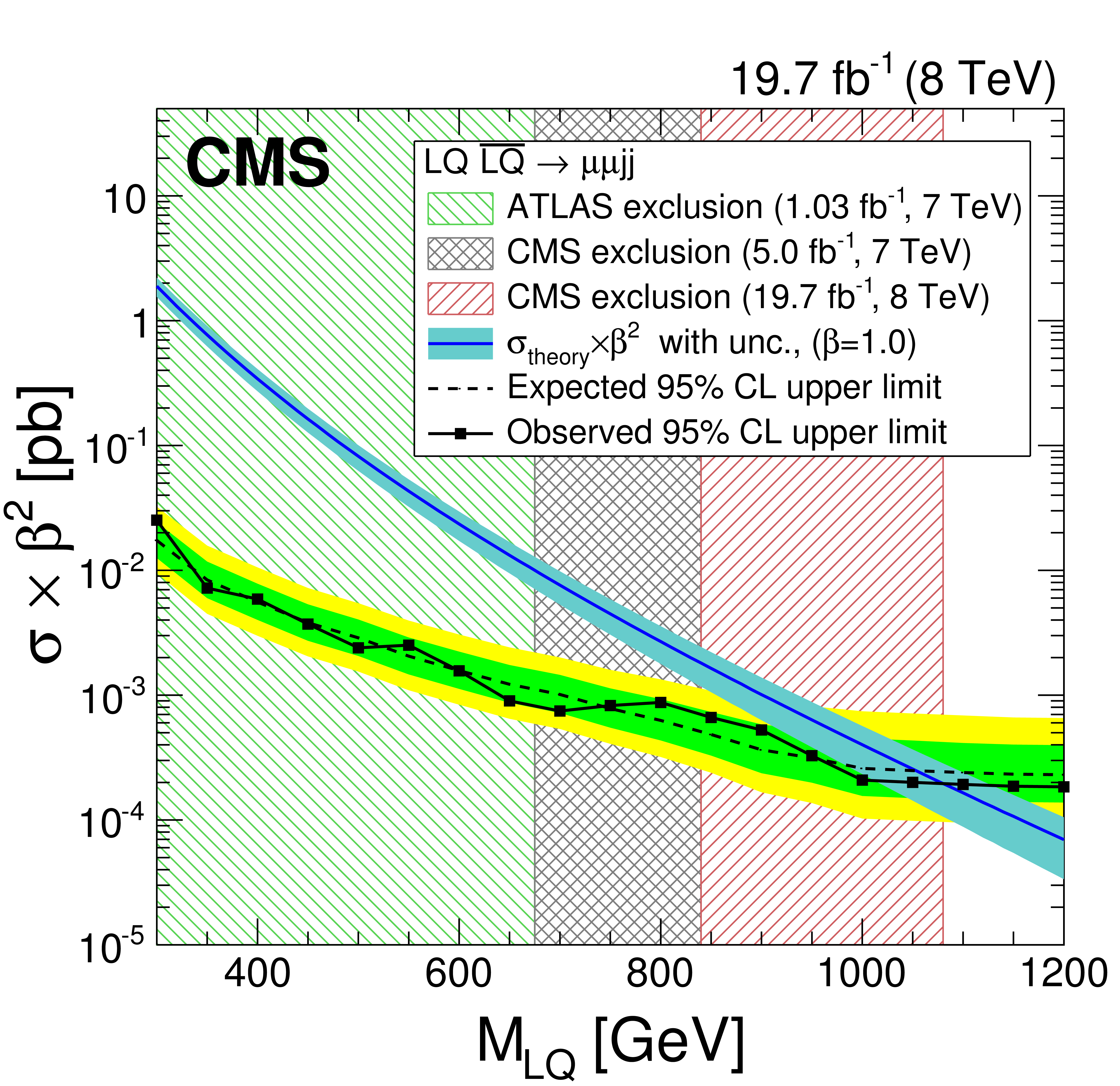
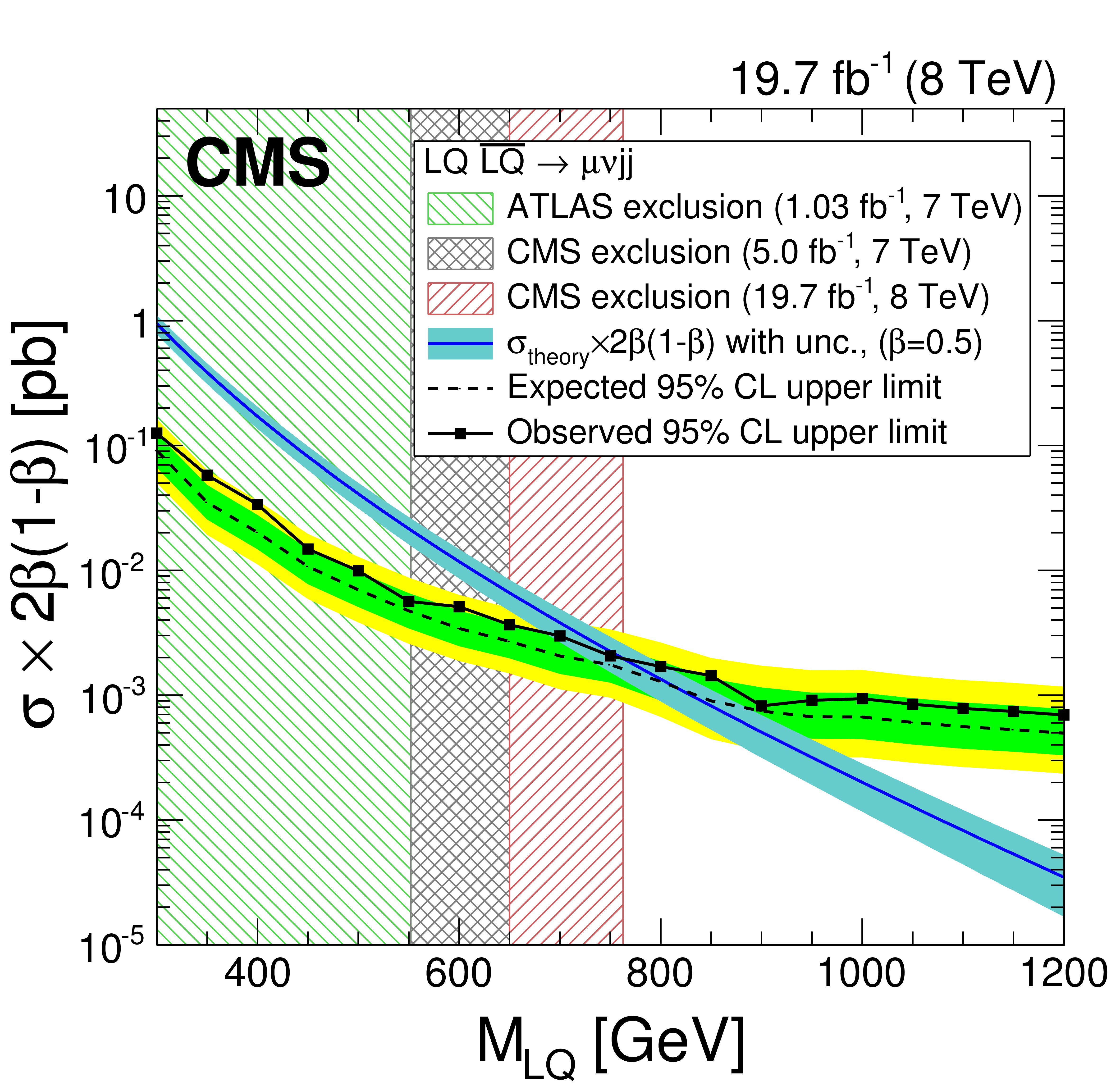
a (b): the expected and observed upper limits at 95% CL on the LQ pair production cross section times $\beta ^2$ ($2\beta (1-\beta )$) as a function of the second generation LQ mass obtained with the $ { {{\mu }} {{\mu }} {\mathrm {j}} {\mathrm {j}} }$ ($ { {{\mu }} {\nu } {\mathrm {j}} {\mathrm {j}} }$) analysis. The expected limits and uncertainty bands represent the median expected limits and the 68% and 95% confidence intervals. The left shaded regions are excluded by Ref.[25] and the middle shaded regions are excluded by Ref.[23]. The right shaded region is excluded by the analysis presented in this paper. The $\sigma _{\rm theory}$ curves and their bands represent, respectively, the theoretical scalar LQ pair production cross section and the uncertainties due to the choice of PDF and renormalization/factorization scales. |
png pdf |
Figure 11-b:
a (b): the expected and observed upper limits at 95% CL on the LQ pair production cross section times $\beta ^2$ ($2\beta (1-\beta )$) as a function of the second generation LQ mass obtained with the $ { {{\mu }} {{\mu }} {\mathrm {j}} {\mathrm {j}} }$ ($ { {{\mu }} {\nu } {\mathrm {j}} {\mathrm {j}} }$) analysis. The expected limits and uncertainty bands represent the median expected limits and the 68% and 95% confidence intervals. The left shaded regions are excluded by Ref.[25] and the middle shaded regions are excluded by Ref.[23]. The right shaded region is excluded by the analysis presented in this paper. The $\sigma _{\rm theory}$ curves and their bands represent, respectively, the theoretical scalar LQ pair production cross section and the uncertainties due to the choice of PDF and renormalization/factorization scales. |
png pdf |
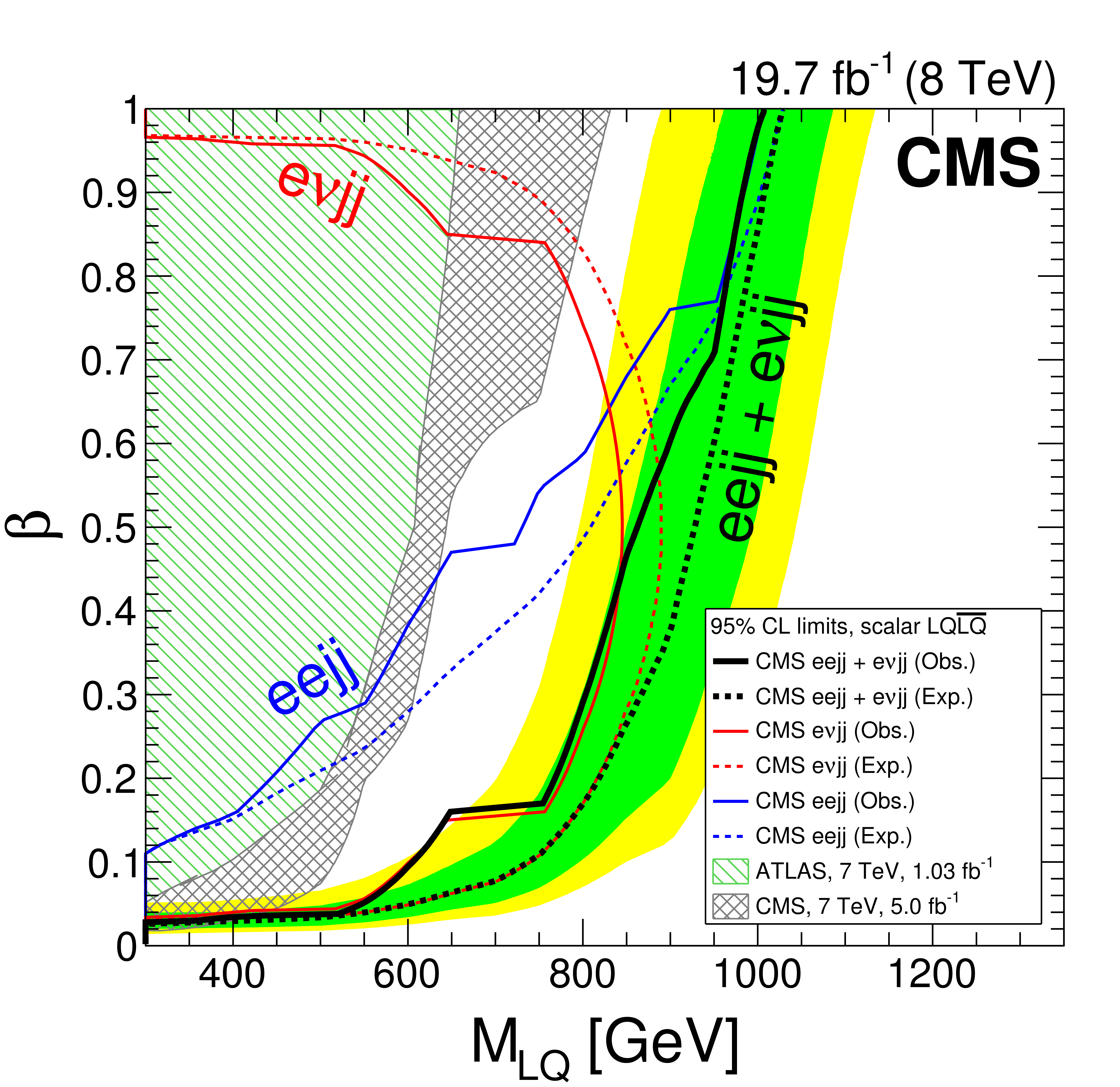
Figure 12-a:
The expected and observed exclusion limits at 95%CL on the first (a) and second (b) generation scalar LQ hypothesis in the $\beta $ versus LQ mass plane using the central value of signal cross section for the individual $ {\mathrm {\ell \ell } {\mathrm {j}} {\mathrm {j}} }$ and $ {\mathrm {\ell } {\nu } {\mathrm {j}} {\mathrm {j}} }$ channels and their combination. The expected limits and uncertainty bands represent the median expected limits and the 68% and 95% confidence intervals. Solid lines represent the observed limits in each channel, and dashed lines represent the expected limits. |
png pdf |
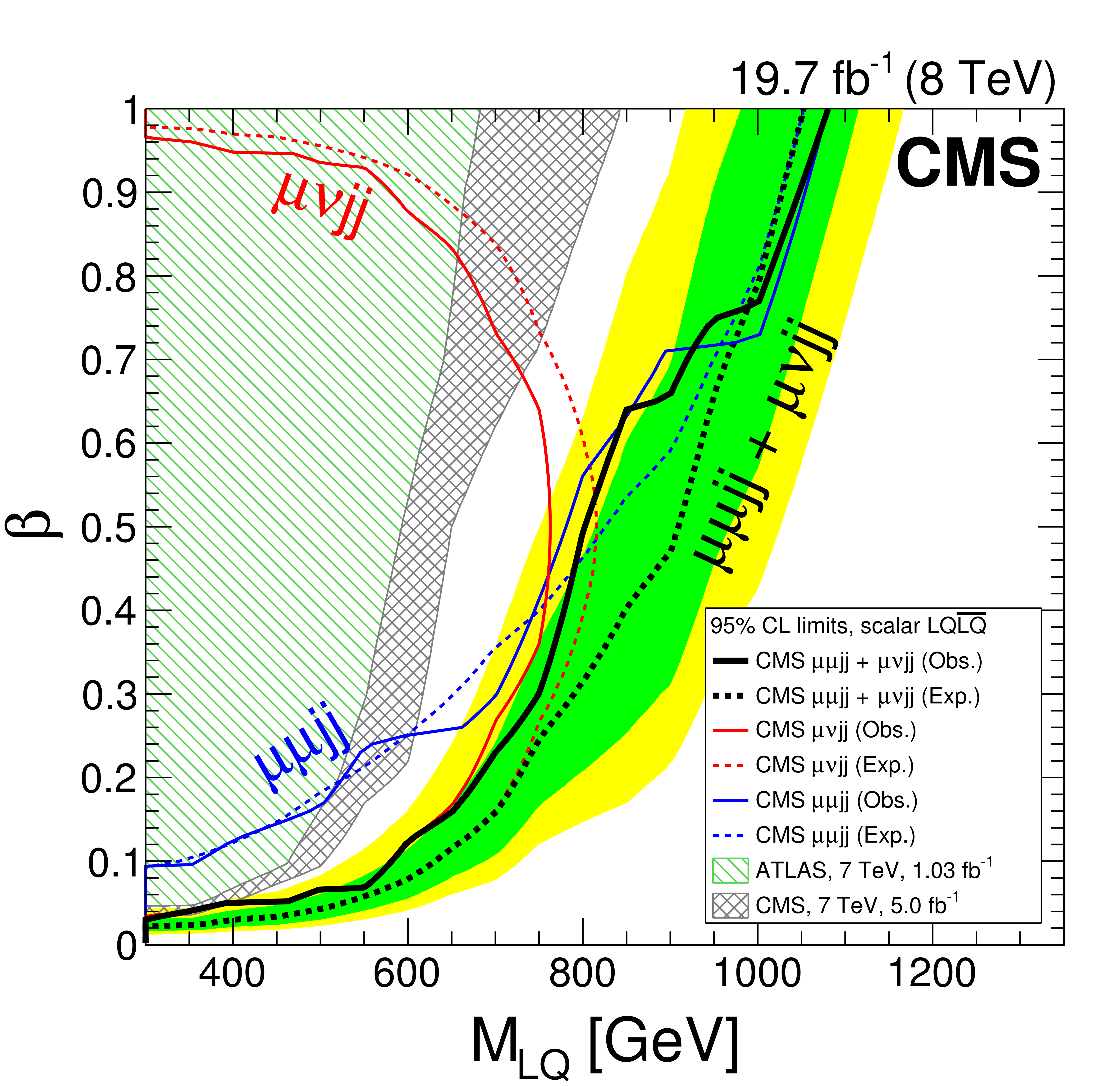
Figure 12-b:
The expected and observed exclusion limits at 95%CL on the first (a) and second (b) generation scalar LQ hypothesis in the $\beta $ versus LQ mass plane using the central value of signal cross section for the individual $ {\mathrm {\ell \ell } {\mathrm {j}} {\mathrm {j}} }$ and $ {\mathrm {\ell } {\nu } {\mathrm {j}} {\mathrm {j}} }$ channels and their combination. The expected limits and uncertainty bands represent the median expected limits and the 68% and 95% confidence intervals. Solid lines represent the observed limits in each channel, and dashed lines represent the expected limits. |

png pdf |
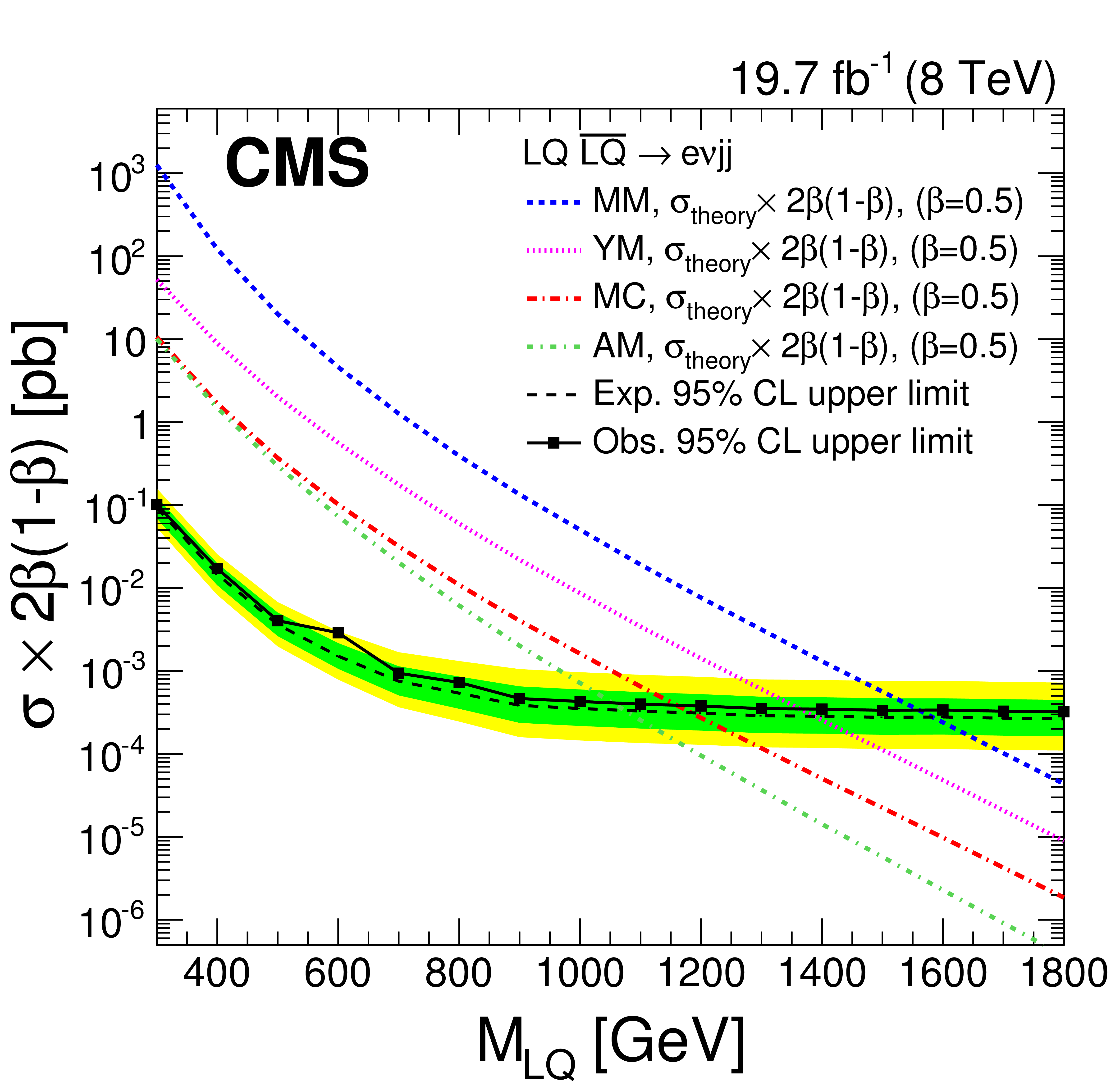
Figure 13-a:
a (b): the expected and observed upper limits at 95% CL on the vector leptoquark pair production cross section times $\beta ^2$ ($2\beta (1-\beta )$) as a function of the first generation vector leptoquark mass, obtained with the $ { {\mathrm {e}} {\mathrm {e}} {\mathrm {j}} {\mathrm {j}} }$ ($ { {\mathrm {e}} {\nu } {\mathrm {j}} {\mathrm {j}} }$) analysis for the four coupling scenarios (MC, YM, MM, and AM). The expected limits and uncertainty bands represent the median expected limits and the 68% and 95% confidence intervals using the MC scenario. Because of the kinematic similarity between the MC scenario and the other coupling scenarios, cross section limits are found to be the same within the uncertainties. |
png pdf |
Figure 13-b:
a (b): the expected and observed upper limits at 95% CL on the vector leptoquark pair production cross section times $\beta ^2$ ($2\beta (1-\beta )$) as a function of the first generation vector leptoquark mass, obtained with the $ { {\mathrm {e}} {\mathrm {e}} {\mathrm {j}} {\mathrm {j}} }$ ($ { {\mathrm {e}} {\nu } {\mathrm {j}} {\mathrm {j}} }$) analysis for the four coupling scenarios (MC, YM, MM, and AM). The expected limits and uncertainty bands represent the median expected limits and the 68% and 95% confidence intervals using the MC scenario. Because of the kinematic similarity between the MC scenario and the other coupling scenarios, cross section limits are found to be the same within the uncertainties. |
png pdf |
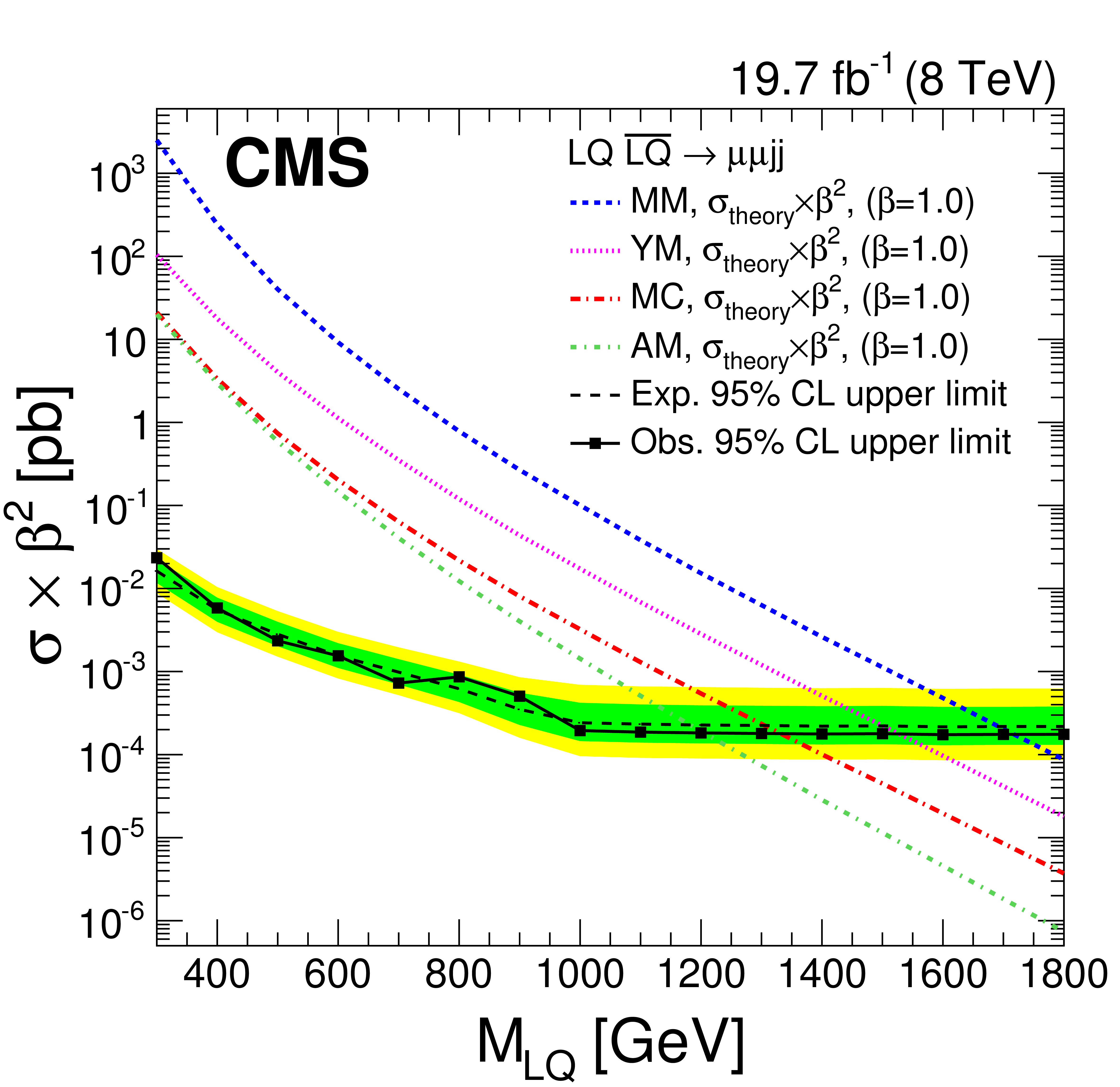
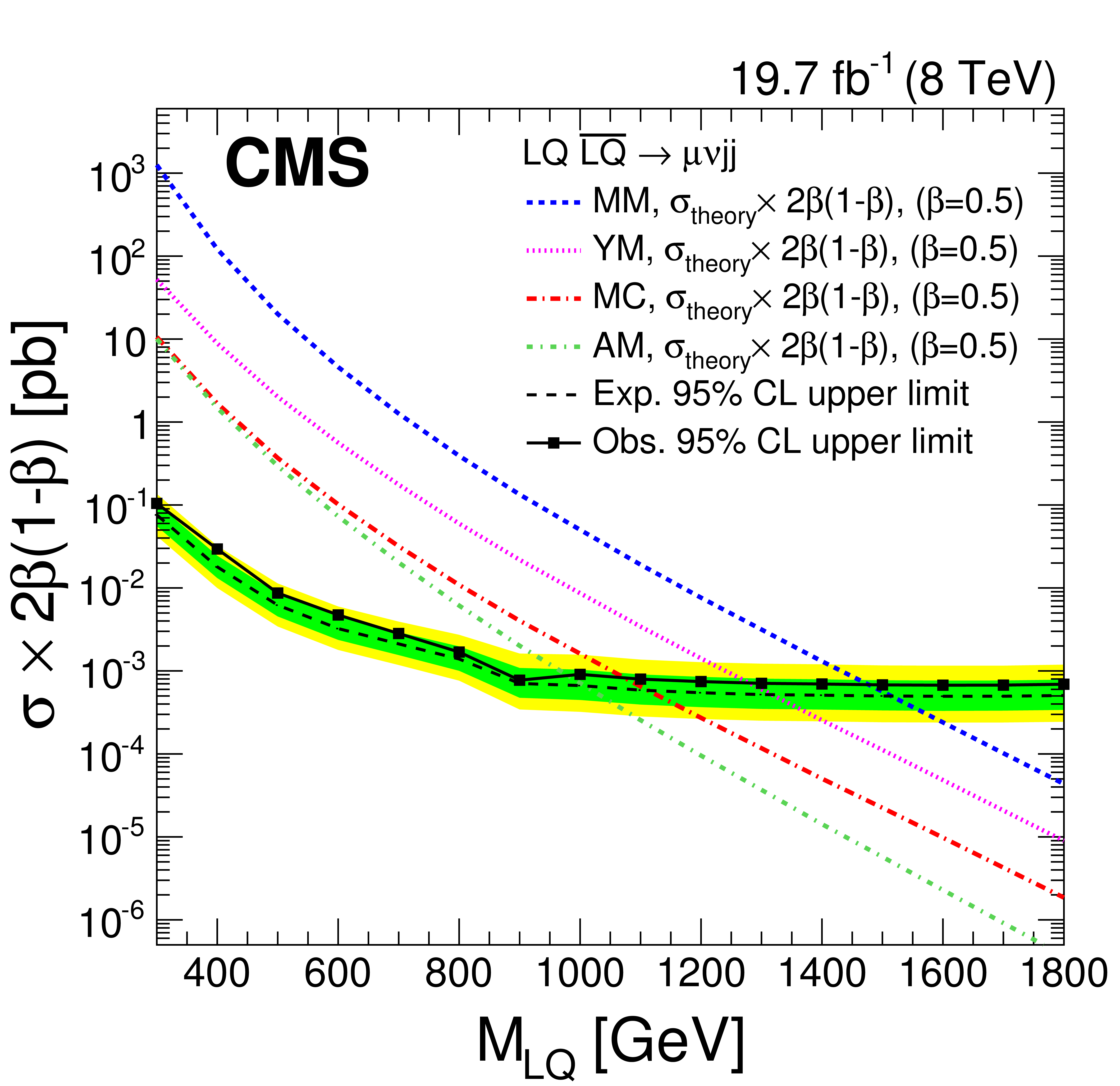
Figure 14-a:
a (b): the expected and observed upper limits at 95% CL on the vector leptoquark pair production cross section times $\beta ^2$ ($2\beta (1-\beta )$) as a function of the second generation vector leptoquark mass, obtained with the $ { {{\mu }} {{\mu }} {\mathrm {j}} {\mathrm {j}} }$ ($ { {{\mu }} {\nu } {\mathrm {j}} {\mathrm {j}} }$) analysis for the four coupling scenarios (MC, YM, MM, and AM). The expected limits and uncertainty bands represent the median expected limits and the 68% and 95% confidence intervals using the MC scenario. Because of the kinematic similarity between the MC scenario and the other coupling scenarios, cross section limits are found to be the same within the uncertainties. |
png pdf |
Figure 14-b:
a (b): the expected and observed upper limits at 95% CL on the vector leptoquark pair production cross section times $\beta ^2$ ($2\beta (1-\beta )$) as a function of the second generation vector leptoquark mass, obtained with the $ { {{\mu }} {{\mu }} {\mathrm {j}} {\mathrm {j}} }$ ($ { {{\mu }} {\nu } {\mathrm {j}} {\mathrm {j}} }$) analysis for the four coupling scenarios (MC, YM, MM, and AM). The expected limits and uncertainty bands represent the median expected limits and the 68% and 95% confidence intervals using the MC scenario. Because of the kinematic similarity between the MC scenario and the other coupling scenarios, cross section limits are found to be the same within the uncertainties. |
png pdf |
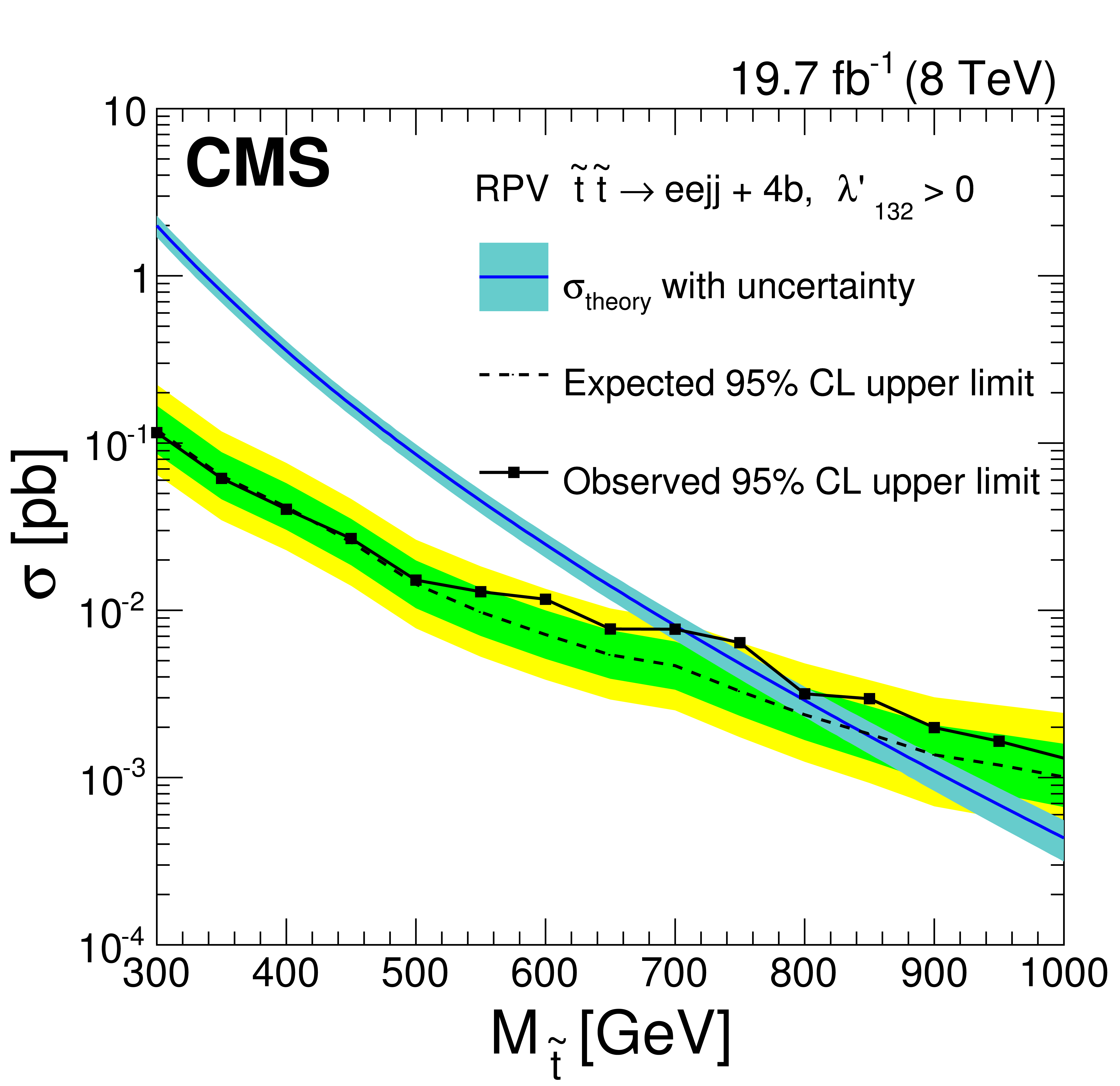
Figure 15-a:
a (b): the expected and observed upper limits at 95% CL on the top squark pair-production cross section for a Higgsino-mediated RPV SUSY model in the ${ {\mathrm {e}} {\mathrm {e}} {\mathrm {j}} {\mathrm {j}} }$ ($ { {{\mu }} {{\mu }} {\mathrm {j}} {\mathrm {j}} }$) + 4b quark final state as a function of the top squark mass, obtained with the $ { {\mathrm {e}} {\mathrm {e}} {\mathrm {j}} {\mathrm {j}} }$ ($ { {{\mu }} {{\mu }} {\mathrm {j}} {\mathrm {j}} }$) analysis. The expected limits and uncertainty bands represent the median expected limits and the 68% and 95% confidence intervals. The $\sigma _{\rm theory}$ curves and their bands represent, respectively, the theoretical top squark pair production cross section and the uncertainties due to the choice of PDF and renormalization/factorization scales. |
png pdf |
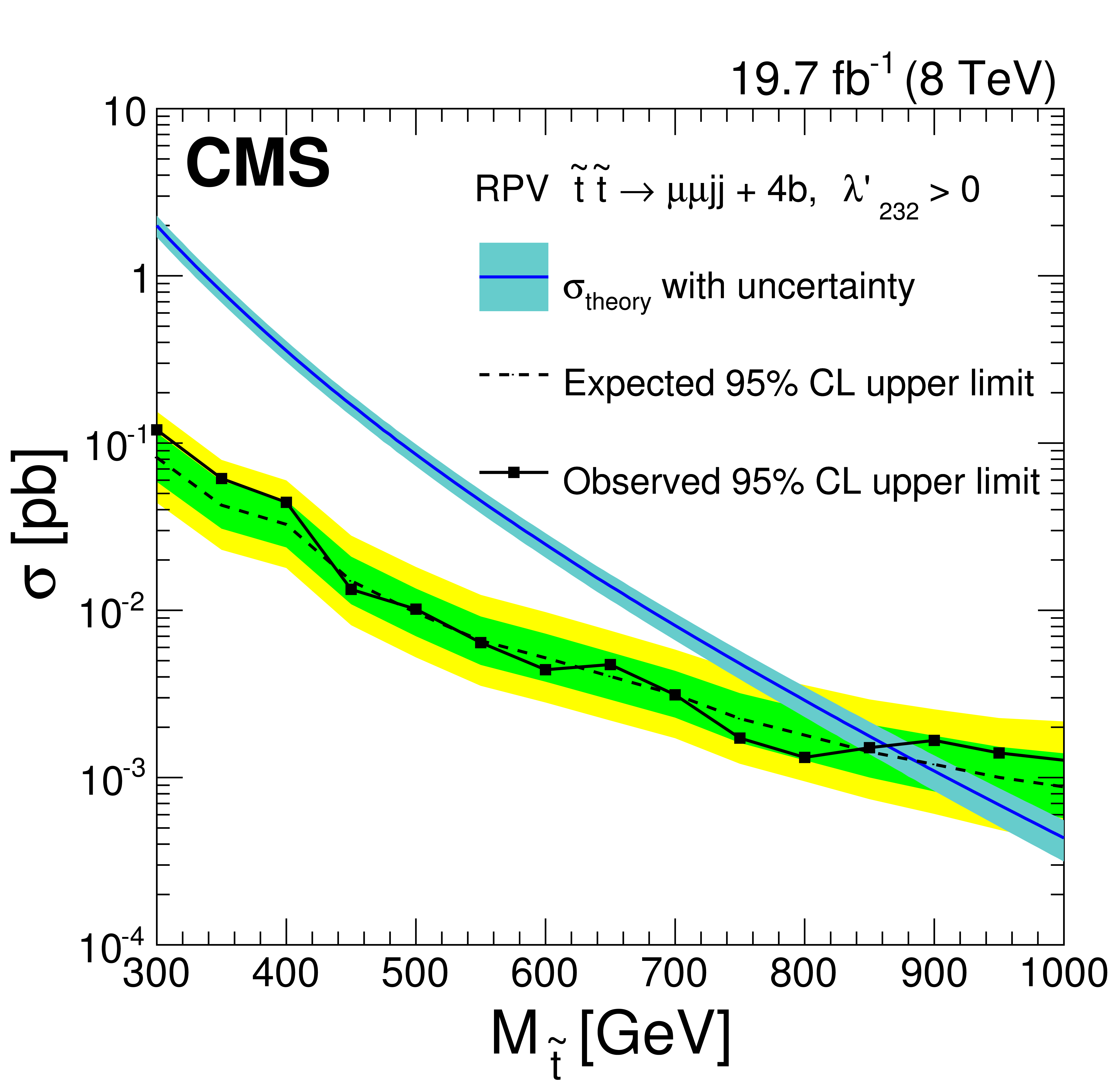
Figure 15-b:
a (b): the expected and observed upper limits at 95% CL on the top squark pair-production cross section for a Higgsino-mediated RPV SUSY model in the ${ {\mathrm {e}} {\mathrm {e}} {\mathrm {j}} {\mathrm {j}} }$ ($ { {{\mu }} {{\mu }} {\mathrm {j}} {\mathrm {j}} }$) + 4b quark final state as a function of the top squark mass, obtained with the $ { {\mathrm {e}} {\mathrm {e}} {\mathrm {j}} {\mathrm {j}} }$ ($ { {{\mu }} {{\mu }} {\mathrm {j}} {\mathrm {j}} }$) analysis. The expected limits and uncertainty bands represent the median expected limits and the 68% and 95% confidence intervals. The $\sigma _{\rm theory}$ curves and their bands represent, respectively, the theoretical top squark pair production cross section and the uncertainties due to the choice of PDF and renormalization/factorization scales. |
| Summary |
| A search has been conducted for pair production of first- and second-generation scalar leptoquarks in final states with either two electrons (or two muons) and two jets, or with one electron (or muon), significant missing transverse energy, and two jets, using 8 TeV proton-proton collision data corresponding to an integrated luminosity of 19.7 fb${-1}$. The results are also interpreted in the context of models of vector leptoquark pair production and of R-parity violating supersymmetric models with similar final state signatures. The selection criteria used for all the searches are optimized for each scalar leptoquark signal mass hypothesis. In the first generation eejj (e$\nu$jj) channel, a broad 2.4 (2.6) standard deviation excess is observed in the final selection optimized for leptoquarks with a mass of 650 GeV. The excess does not peak in the $M_{\mathrm{ejj}}$ distributions, as a leptoquark signal would, but does weaken the upper limit that can be set on the production cross section for leptoquark masses of about 650 GeV and values of $\beta <$ 0.15. Limits are placed with 95% CL on first-generation scalar leptoquarks with masses less than 1010 (850) GeV, assuming $\beta = $ 1.0 (0.5). This is to be compared with the expected 95% CL exclusions of 1030 (890) GeV. In the secondgeneration leptoquark search the number of observed candidates for each mass hypothesis agrees within uncertainties with the number of expected standard model background events. Second-generation scalar leptoquarks are excluded at 95% CL with masses below 1080 (800) GeV for $\beta = 1.0$~$(0.5)$. This is to be compared with a median expected limit of 1050 (910) GeV. The limits for $\beta = $1.0 and 0.5 represent the most stringent limits on first- and second-generation scalar leptoquarks to date.Limits are set on four coupling scenarios for vector leptoquarks, and for the eejj (e$\nu$jj) channel yield 95% CL upper limit exclusions of masses in the range of 1150-1660 (1050-1560) GeV. In the $\mu\mu$jj ($\mu\nu$jj) channel, the experimental results yield 95% CL upper limit exclusions of masses in the range of 1200-1720 (980-1480) GeV. These represent the most stringent limits on vector LQ production to date.Limits are also set for top squark production in an R-parity violating supersymmetric model via the $\lambda^{\prime}_{132}$ or $\lambda^{\prime}_{232}$ operators. For direct top squark decay, the scalar LQ limits can be applied directly. Interpretation is also made in Higgsino-mediated top squark decay, where the experimental results yield a 95% CL observed upper limit exclusion of top squark masses less than 710 GeV in the first generation $\lambda^{\prime}_{132}$ model, compared with a median expected limit of 840 GeV. The second generation $\lambda^{\prime}_{232}$ model yields an observed exclusion of top squark masses less than 860 GeV, compared with a median expected limit of 880 GeV. These represent the most stringent experimental limits to date on $\lambda^{\prime}_{132}$ and $\lambda^{\prime}_{232}$ RPV SUSY top squark decays and the first experimental limits on the Higgsino-mediated decays. |
|
|
Compact Muon Solenoid LHC, CERN |
|

|

|

|

|

|