

Compact Muon Solenoid
LHC, CERN
| CMS-EXO-12-060 ; CERN-PH-EP-2014-176 | ||
| Search for physics beyond the standard model in final states with a lepton and missing transverse energy in proton-proton collisions at $\sqrt{s}$ = 8 TeV | ||
| CMS Collaboration | ||
| 13 August 2014 | ||
| Phys. Rev. D 91 (2015) 092005 | ||
| Abstract: A search for new physics in proton-proton collisions having final states with an electron or muon and missing transverse energy is presented. The analysis uses data collected in 2012 with the CMS detector, at an LHC center-of-mass energy of 8 TeV, and corresponding to an integrated luminosity of 19.7 fb$^{-1}$. No significant deviation of the transverse mass distribution of the charged lepton-neutrino system from the standard model prediction is found. Mass exclusion limits of up to 3.28 TeV at a 95% confidence level for a W$^{\prime}$ boson with the same couplings as that of the standard model W boson are determined. Results are also derived in the framework of split universal extra dimensions, and exclusion limits on Kaluza-Klein W$^{(2)}_{{\rm KK}}$ states are found. The final state with large missing transverse energy also enables a search for dark matter production with a recoiling W boson, with limits set on the mass and the production cross section of potential candidates. Finally, limits are established for a model including interference between a left-handed W$^{\prime}$ boson and the standard model W boson, and for a compositeness model. | ||
| Links: e-print arXiv:1408.2745 [hep-ex] (PDF) ; CDS record ; inSPIRE record ; Public twiki page ; CADI line (restricted) ; | ||
| Figures | |
png pdf |
Figure 1:
Production and decay of an SSM W' or $ {\mathrm {W}_\mathrm {KK}} $ boson (left); HNC-CI (center); DM single W boson production (right). |
png pdf |
Figure 2:
Feynman diagrams for dark matter interference, shown as an example with an up and a down quark. The same initial and final state can have different particles coupling to the dark matter particles. |
png pdf |
Figure 3-a:
Signal shapes at generator level: SSM model compared to the SSMS and SSMO models for $g_{ {\mathrm {W}^\prime } }/g_{ {\mathrm {W}} }=1$ (a); HNC-CI model for various values of $\Lambda $ (b); DM for various values of $\xi $ (c); W' with W boson interference and a varying coupling strength $g_{ {\mathrm {W}}}/g_{ {\mathrm {W}^\prime } }$ in the same sign scenario (d); and TeV$^{-1}$ model (e). |
png pdf |
Figure 3-b:
Signal shapes at generator level: SSM model compared to the SSMS and SSMO models for $g_{ {\mathrm {W}^\prime } }/g_{ {\mathrm {W}} }=1$ (a); HNC-CI model for various values of $\Lambda $ (b); DM for various values of $\xi $ (c); W' with W boson interference and a varying coupling strength $g_{ {\mathrm {W}}}/g_{ {\mathrm {W}^\prime } }$ in the same sign scenario (d); and TeV$^{-1}$ model (e). |
png pdf |
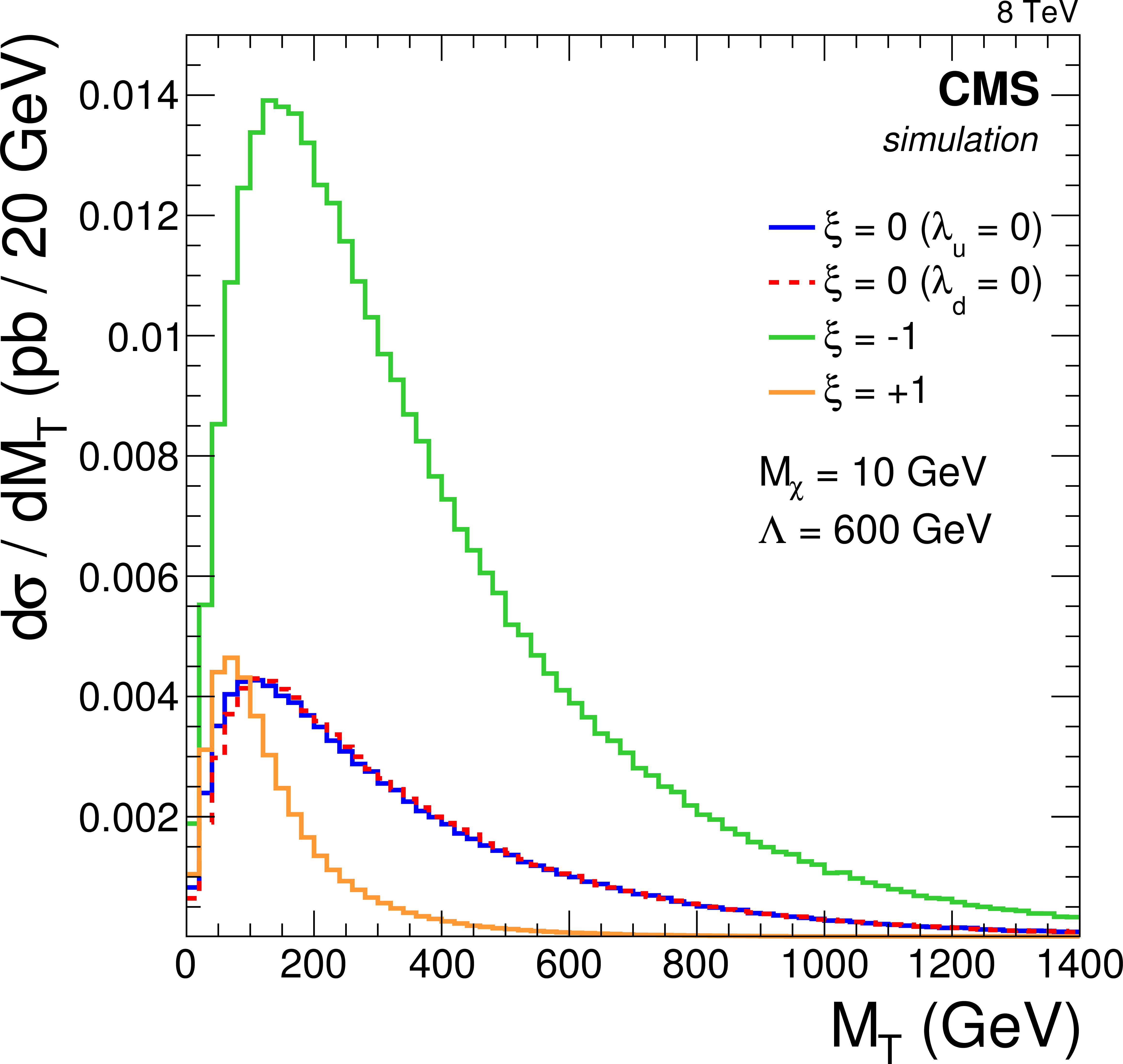
Figure 3-c:
Signal shapes at generator level: SSM model compared to the SSMS and SSMO models for $g_{ {\mathrm {W}^\prime } }/g_{ {\mathrm {W}} }=1$ (a); HNC-CI model for various values of $\Lambda $ (b); DM for various values of $\xi $ (c); W' with W boson interference and a varying coupling strength $g_{ {\mathrm {W}}}/g_{ {\mathrm {W}^\prime } }$ in the same sign scenario (d); and TeV$^{-1}$ model (e). |

png pdf |
Figure 3-d:
Signal shapes at generator level: SSM model compared to the SSMS and SSMO models for $g_{ {\mathrm {W}^\prime } }/g_{ {\mathrm {W}} }=1$ (a); HNC-CI model for various values of $\Lambda $ (b); DM for various values of $\xi $ (c); W' with W boson interference and a varying coupling strength $g_{ {\mathrm {W}}}/g_{ {\mathrm {W}^\prime } }$ in the same sign scenario (d); and TeV$^{-1}$ model (e). |
png pdf |
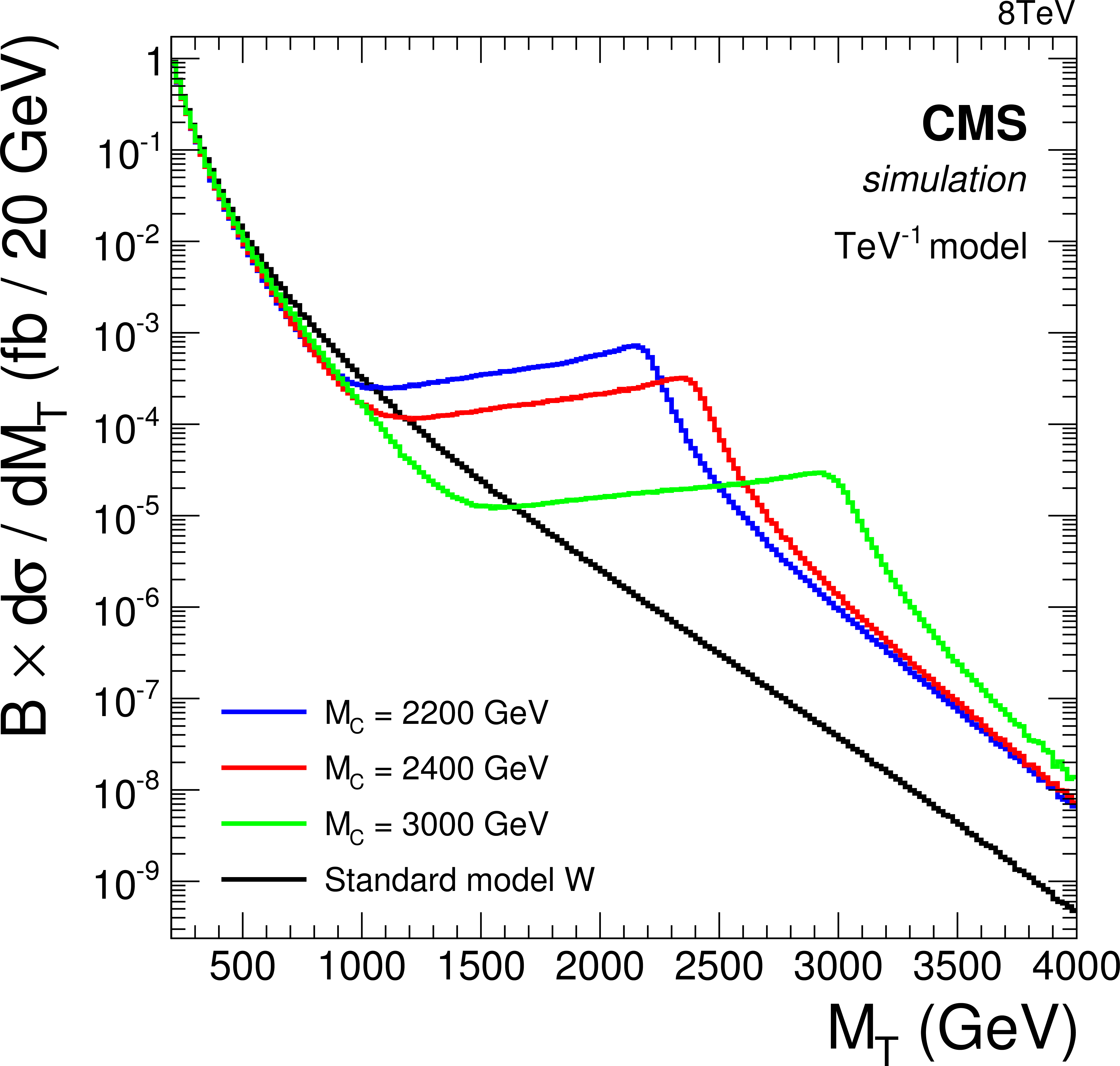
Figure 3-e:
Signal shapes at generator level: SSM model compared to the SSMS and SSMO models for $g_{ {\mathrm {W}^\prime } }/g_{ {\mathrm {W}} }=1$ (a); HNC-CI model for various values of $\Lambda $ (b); DM for various values of $\xi $ (c); W' with W boson interference and a varying coupling strength $g_{ {\mathrm {W}}}/g_{ {\mathrm {W}^\prime } }$ in the same sign scenario (d); and TeV$^{-1}$ model (e). |
png pdf |
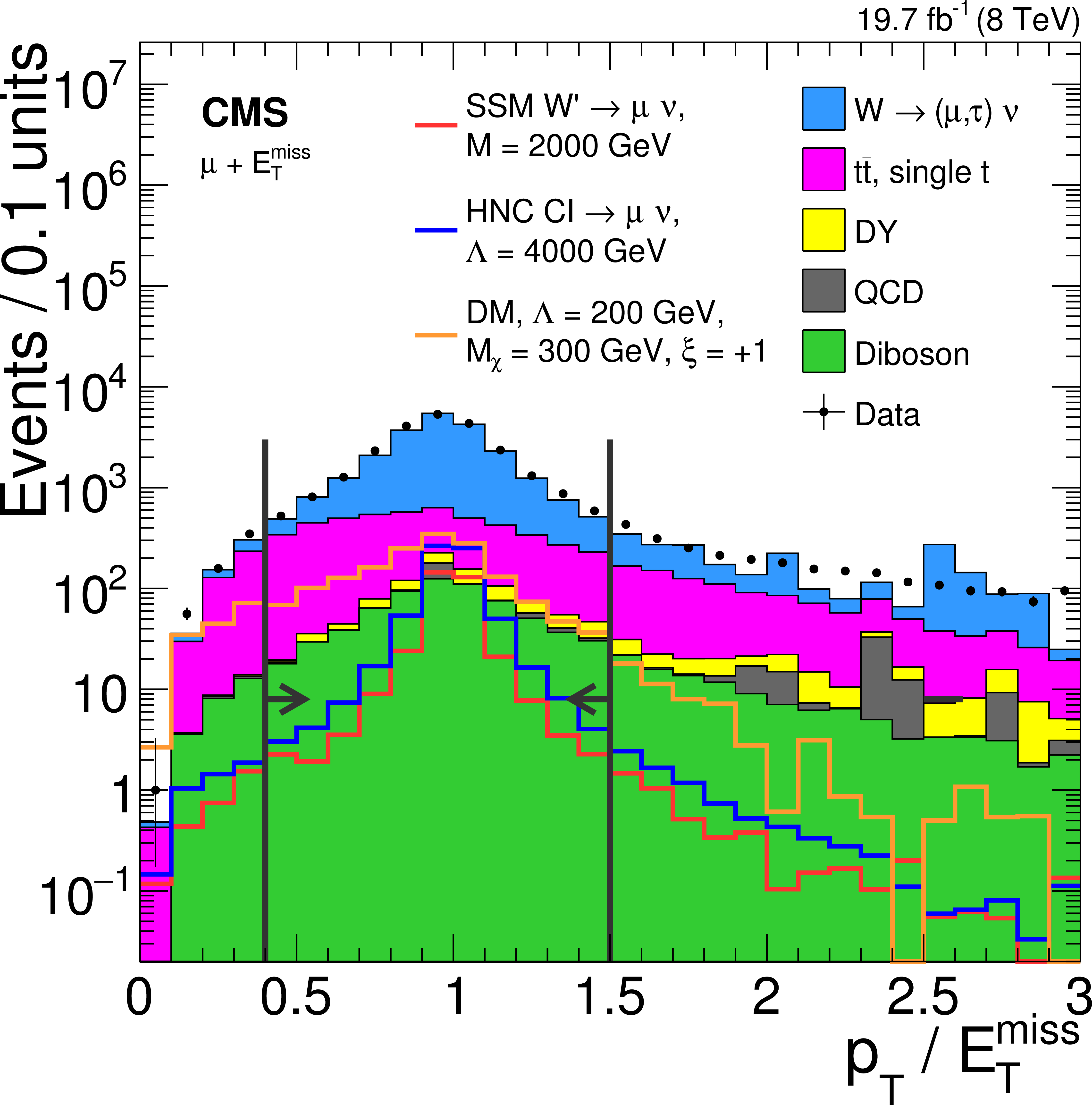
Figure 4-a:
The distribution in $ {p_{\mathrm {T}}} / {E_{\mathrm {T}}^{\text {miss}}} $ (a) and $\Delta \phi (\ell , \vec{p}_{\text {T}}^{\text {miss}} )$ (b), for data, background, and some signals in the muon channel with an $ {M_\mathrm {T}} $ threshold of 220 GeV. The simulated background labeled as `diboson' includes $ {\mathrm {W}} {\mathrm {W}}$, $ {\mathrm {Z}} {\mathrm {Z}} $ and $ {\mathrm {W}} {\mathrm {Z}} $ contributions, while `DY' denotes the Drell--Yan process. |
png pdf |
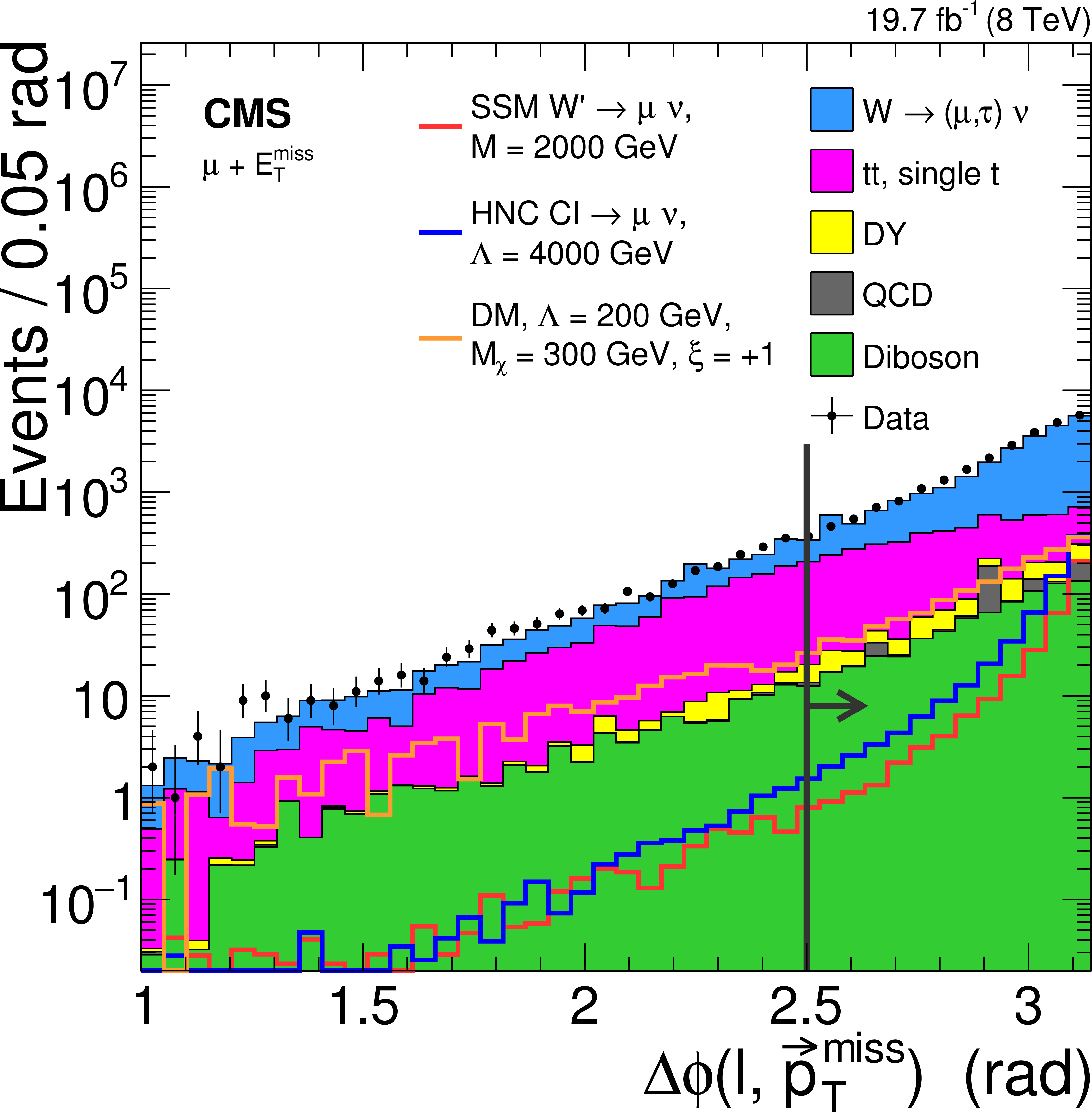
Figure 4-b:
The distribution in $ {p_{\mathrm {T}}} / {E_{\mathrm {T}}^{\text {miss}}} $ (a) and $\Delta \phi (\ell , \vec{p}_{\text {T}}^{\text {miss}} )$ (b), for data, background, and some signals in the muon channel with an $ {M_\mathrm {T}} $ threshold of 220 GeV. The simulated background labeled as `diboson' includes $ {\mathrm {W}} {\mathrm {W}}$, $ {\mathrm {Z}} {\mathrm {Z}} $ and $ {\mathrm {W}} {\mathrm {Z}} $ contributions, while `DY' denotes the Drell--Yan process. |

png pdf |
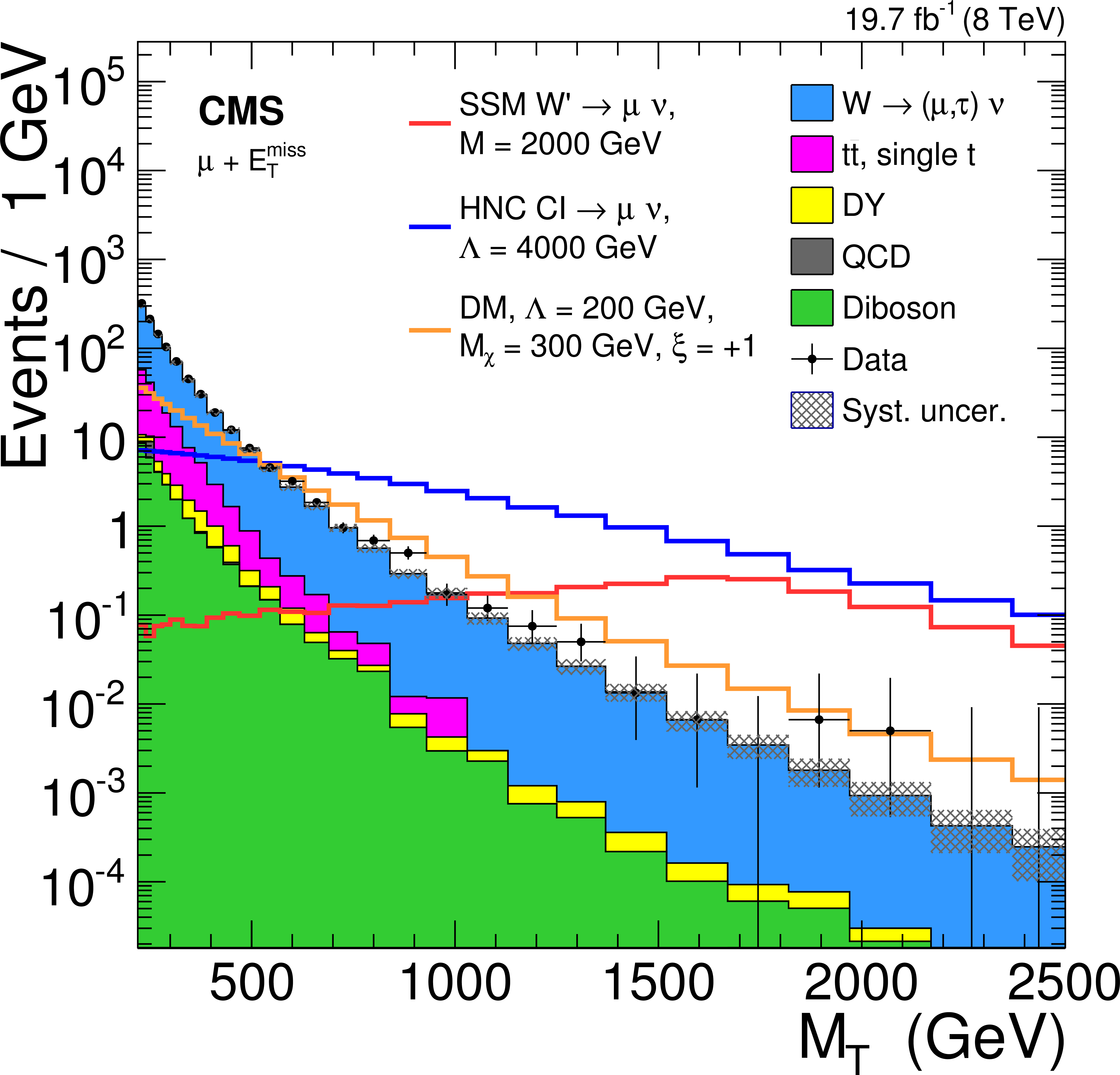
Figure 5-a:
Observed $ {M_\mathrm {T}} $ distributions for the electron (a) and muon (b) channels. The horizontal bars on the data points indicate the widths of the bins. The asymmetric error bars indicate the central confidence intervals for Poisson-distributed data and are obtained from the Neyman construction as described in Ref.[]. |
png pdf |
Figure 5-b:
Observed $ {M_\mathrm {T}} $ distributions for the electron (a) and muon (b) channels. The horizontal bars on the data points indicate the widths of the bins. The asymmetric error bars indicate the central confidence intervals for Poisson-distributed data and are obtained from the Neyman construction as described in Ref.[]. |
png pdf |
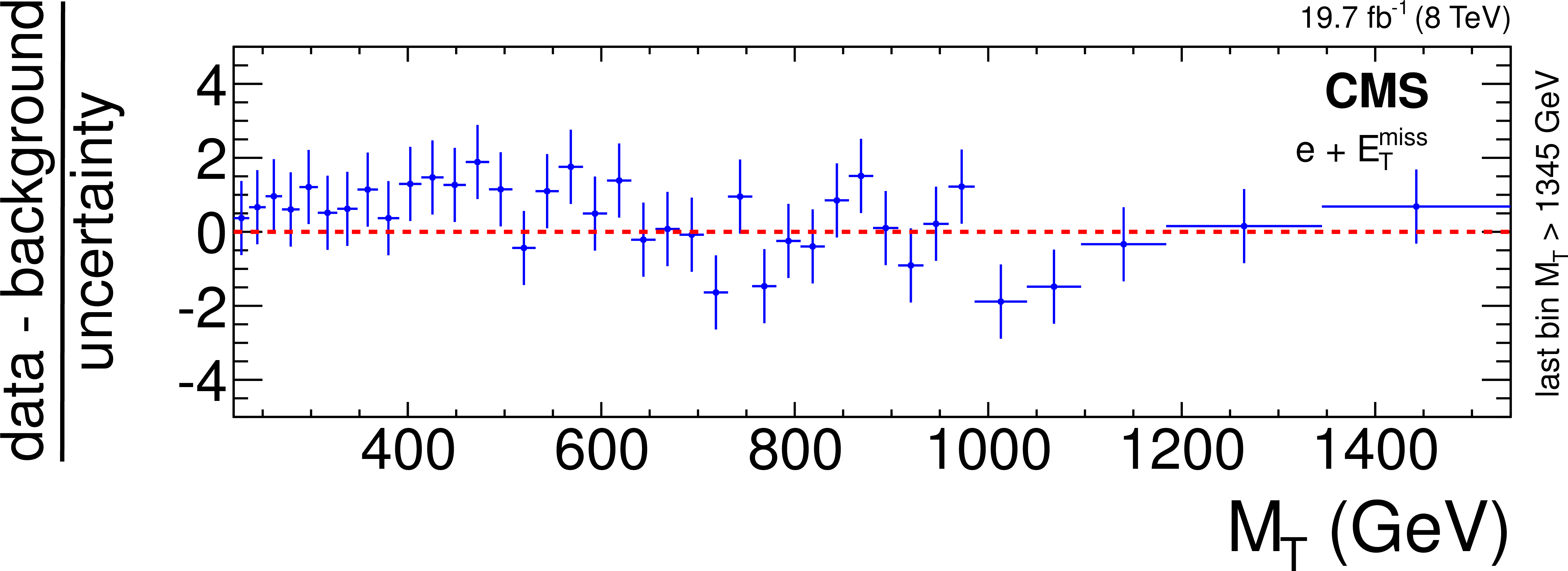
Figure 6-a:
Deviation of the number of observed events from the expectation, as shown in Fig.5, in units of standard deviations, binned in $ {M_\mathrm {T}} $ for the electron (a) and muon (b) channels. Both the systematic and statistical uncertainties are included. The horizontal bars on the data points indicate the widths of the bins, which are chosen as in Fig {fig:MT} with the extension to include always 5 background events in a bin. |

png pdf |
Figure 6-b:
Deviation of the number of observed events from the expectation, as shown in Fig.5, in units of standard deviations, binned in $ {M_\mathrm {T}} $ for the electron (a) and muon (b) channels. Both the systematic and statistical uncertainties are included. The horizontal bars on the data points indicate the widths of the bins, which are chosen as in Fig {fig:MT} with the extension to include always 5 background events in a bin. |
png pdf |
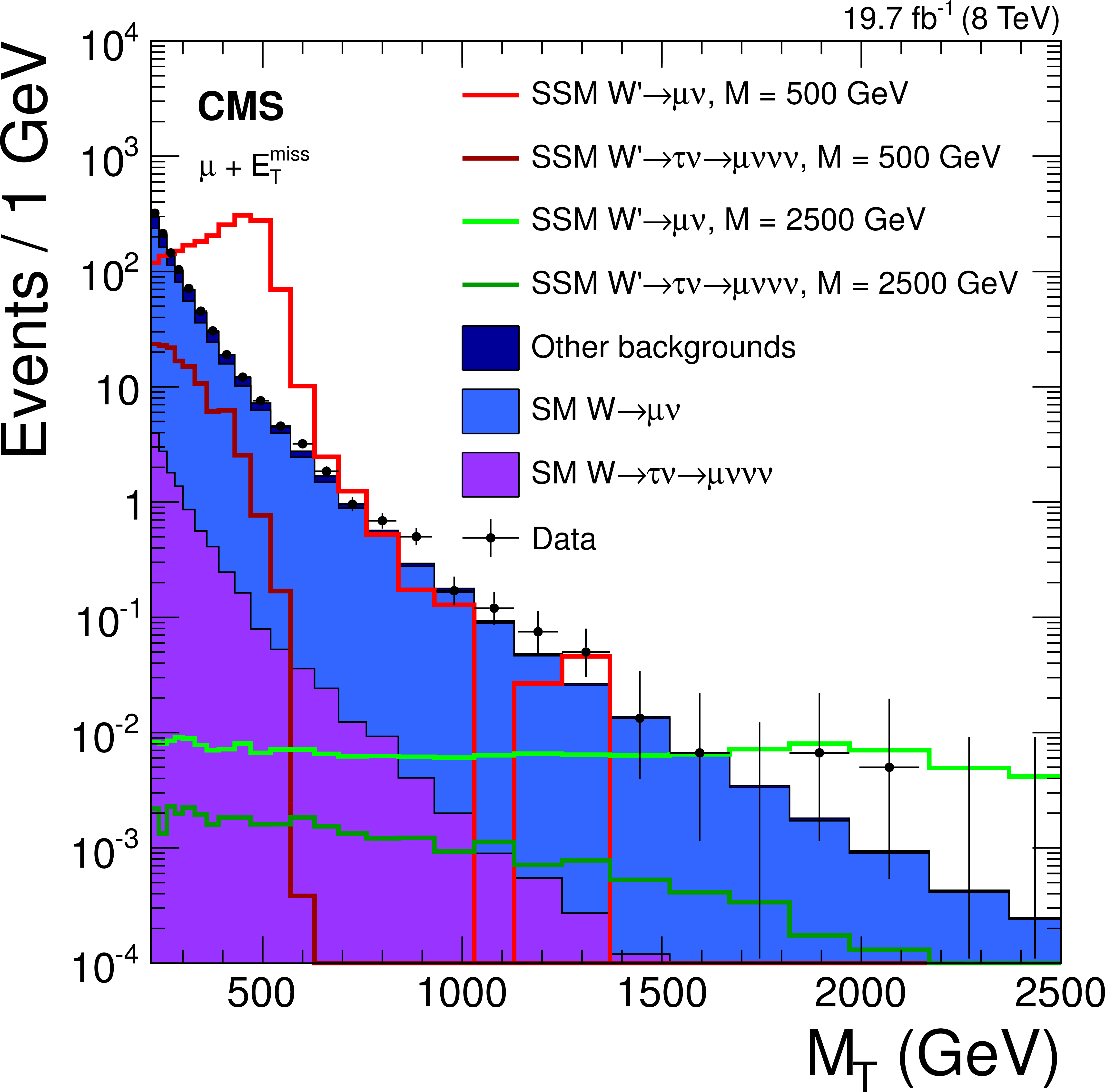
Figure 7:
Contributions from Wand W' bosons decaying to $\tau \nu \to \mu \nu \nu \nu $ compared to the prompt $\mu \nu $ decay channel. Also shown are the contributions from the other backgrounds and the number of data events. The horizontal bars on the data points indicate the widths of the bins. |
png pdf |
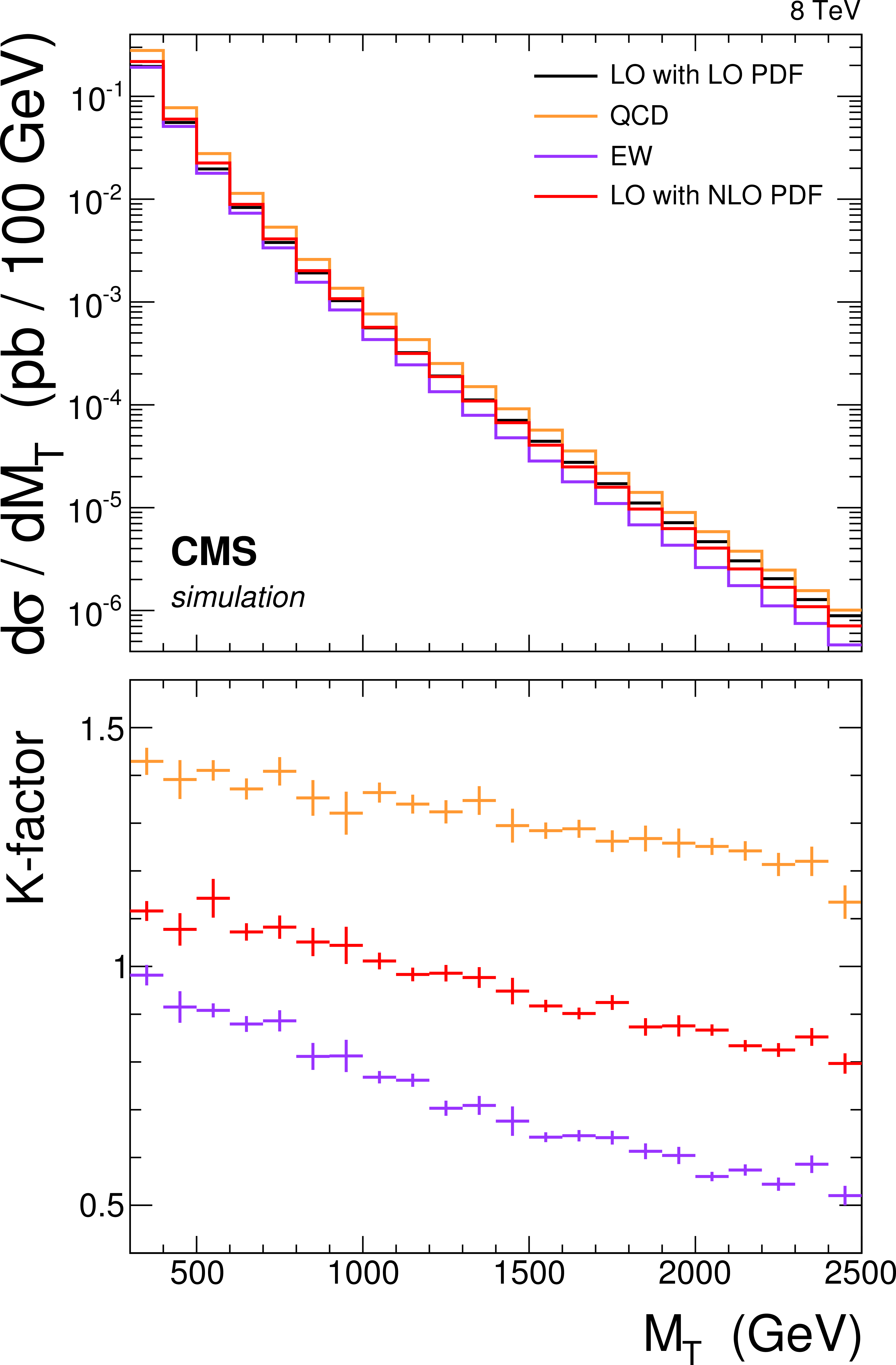
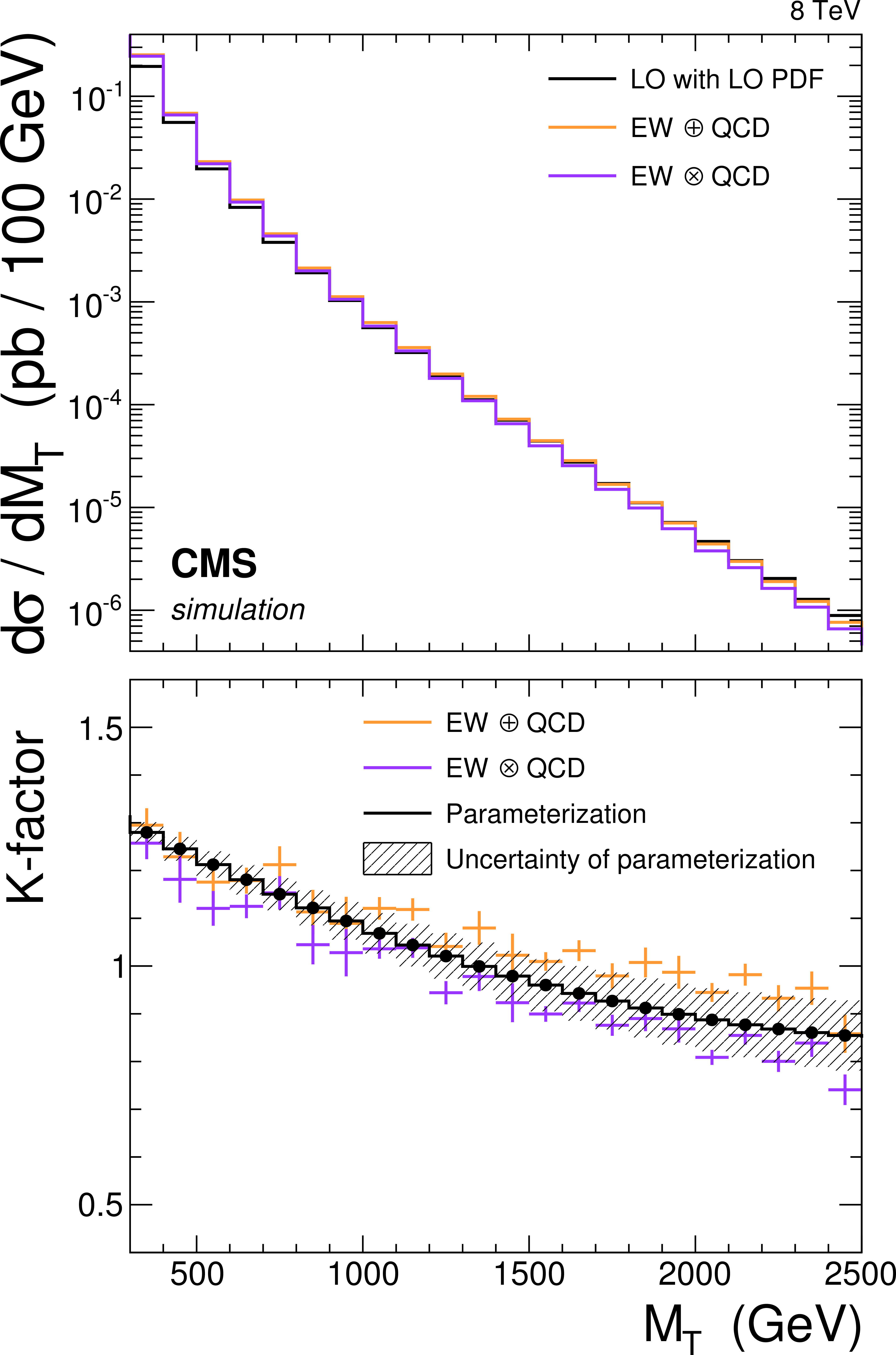
Figure 8-a:
Electroweak and QCD corrections to the SM W-boson background prediction. a: QCD and electroweak contributions compared to the LO calculation with LO PDF. b: Combination of higher-order corrections with an additive and a multiplicative approach compared to the LO calculation with LO PDF, as well as a parameterization of the mean of the values obtained by the two methods. To derive the K-factor data on the right plot, one divides the sum or product of the K-factors on the left plot by the NLO/LO PDF K-factor. |
png pdf |
Figure 8-b:
Electroweak and QCD corrections to the SM W-boson background prediction. a: QCD and electroweak contributions compared to the LO calculation with LO PDF. b: Combination of higher-order corrections with an additive and a multiplicative approach compared to the LO calculation with LO PDF, as well as a parameterization of the mean of the values obtained by the two methods. To derive the K-factor data on the right plot, one divides the sum or product of the K-factors on the left plot by the NLO/LO PDF K-factor. |
png pdf |
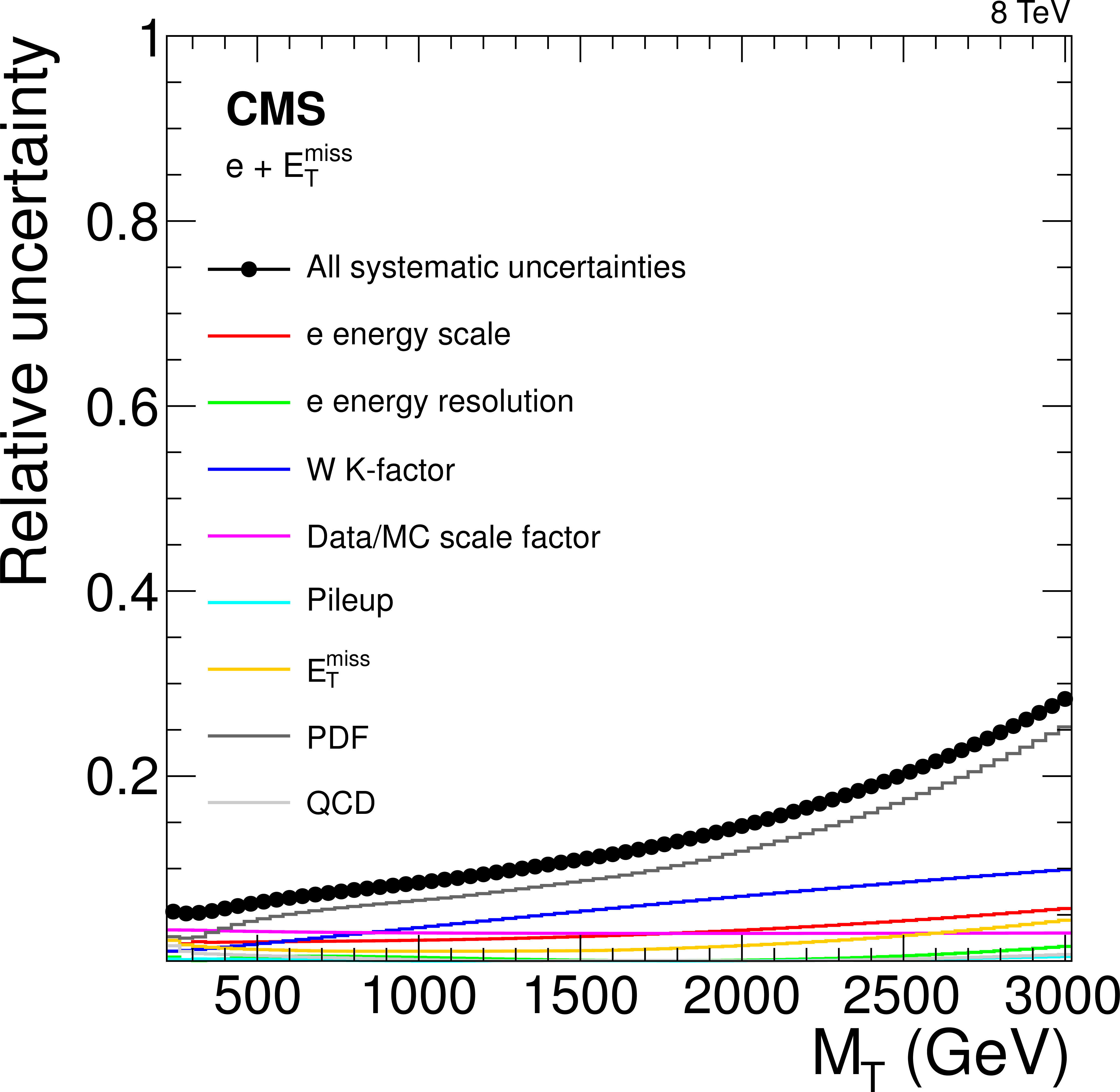
Figure 9-a:
Individual contributions of relative systematic uncertainties on the background event yields in the electron (a) and muon (b) channels. |
png pdf |
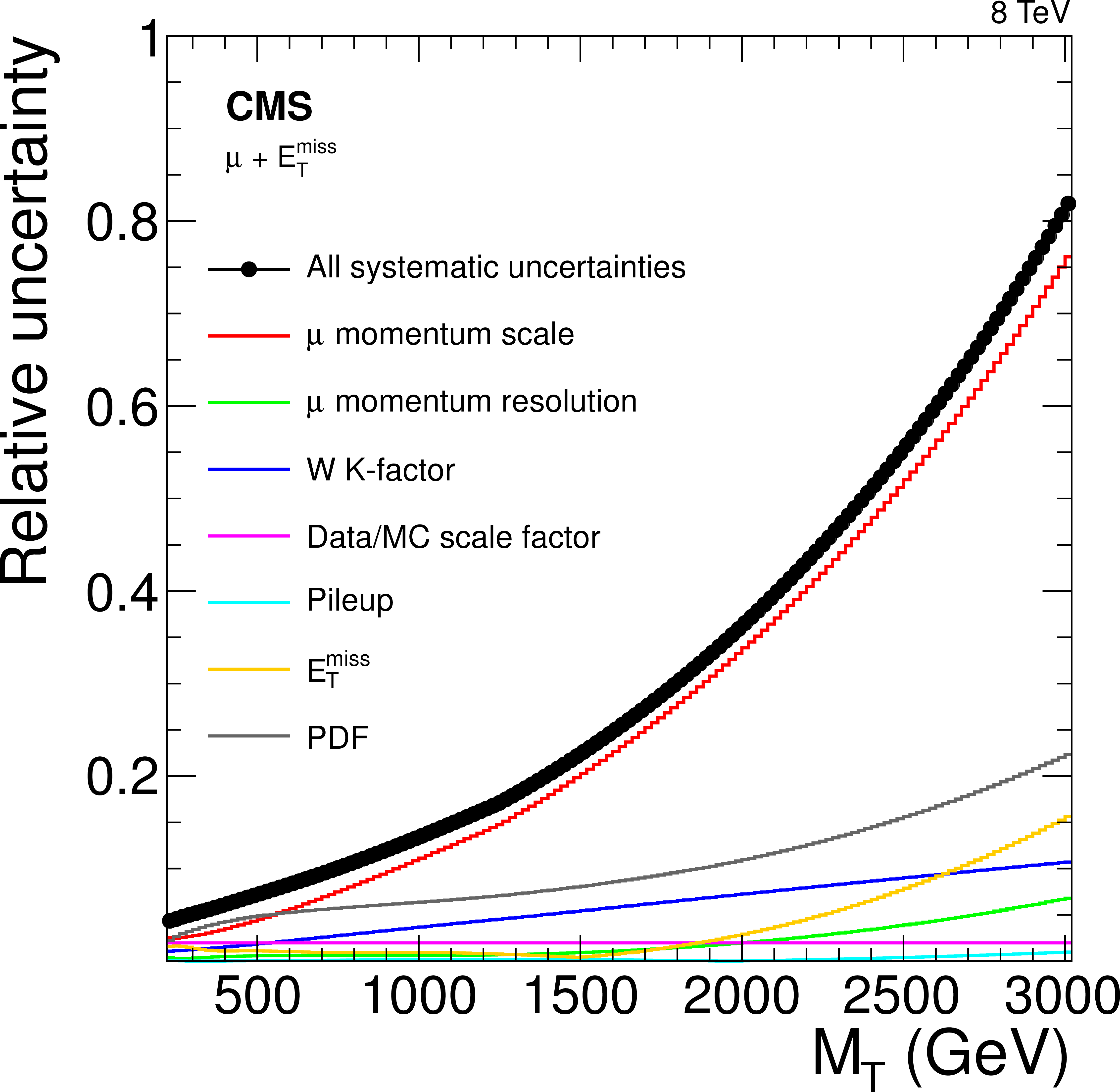
Figure 9-b:
Individual contributions of relative systematic uncertainties on the background event yields in the electron (a) and muon (b) channels. |
png pdf |
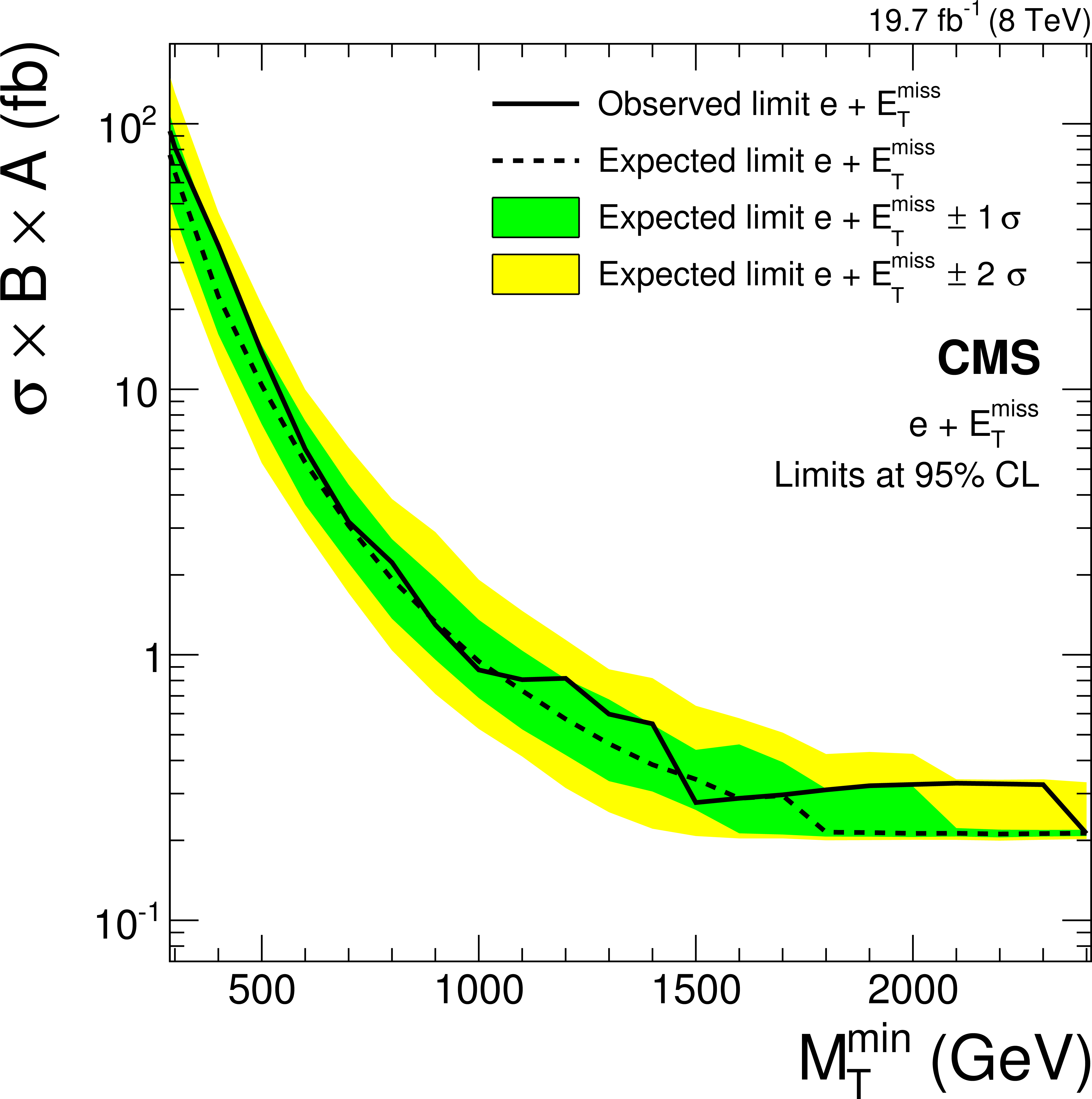
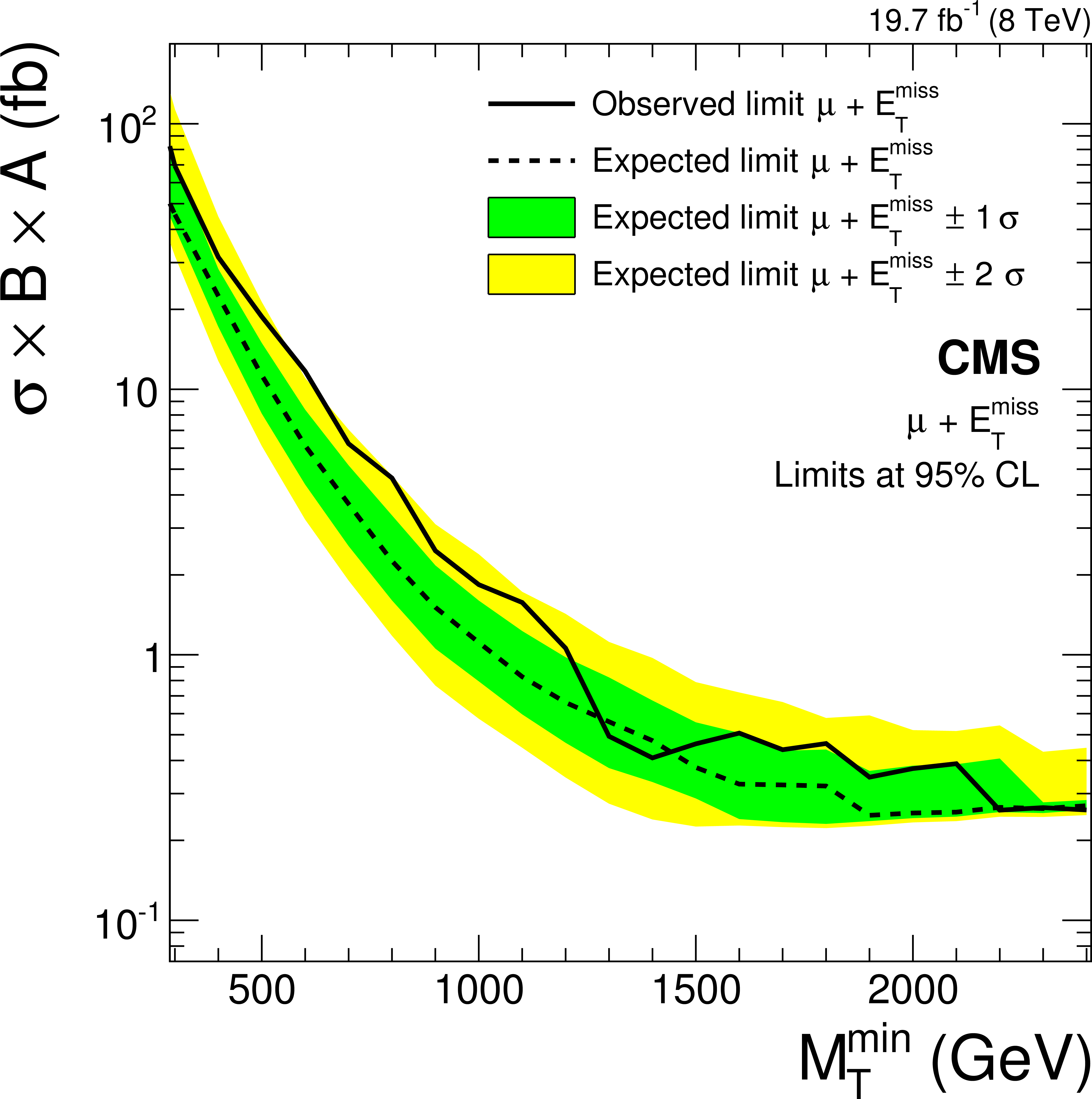
Figure 10-a:
Cross section upper limits at 95% CL on the effective cross section $\sigma ( {\mathrm {W}^\prime } ) \mathcal {B}( {\mathrm {W}^\prime } \to \ell \nu )A$ above a threshold $ {M_\mathrm {T}^\mathrm {min}} $ for the individual electron and muon channels. Shown are the observed limit, expected limit, and the expected limit $1\sigma $ and $2\sigma $ intervals. Only detector acceptance is taken into account for the signal. The parameter $A$ describes the efficiency derived from the kinematic selection criteria and the $ {M_\mathrm {T}^\mathrm {min}} $ threshold. |
png pdf |
Figure 10-b:
Cross section upper limits at 95% CL on the effective cross section $\sigma ( {\mathrm {W}^\prime } ) \mathcal {B}( {\mathrm {W}^\prime } \to \ell \nu )A$ above a threshold $ {M_\mathrm {T}^\mathrm {min}} $ for the individual electron and muon channels. Shown are the observed limit, expected limit, and the expected limit $1\sigma $ and $2\sigma $ intervals. Only detector acceptance is taken into account for the signal. The parameter $A$ describes the efficiency derived from the kinematic selection criteria and the $ {M_\mathrm {T}^\mathrm {min}} $ threshold. |
png pdf |
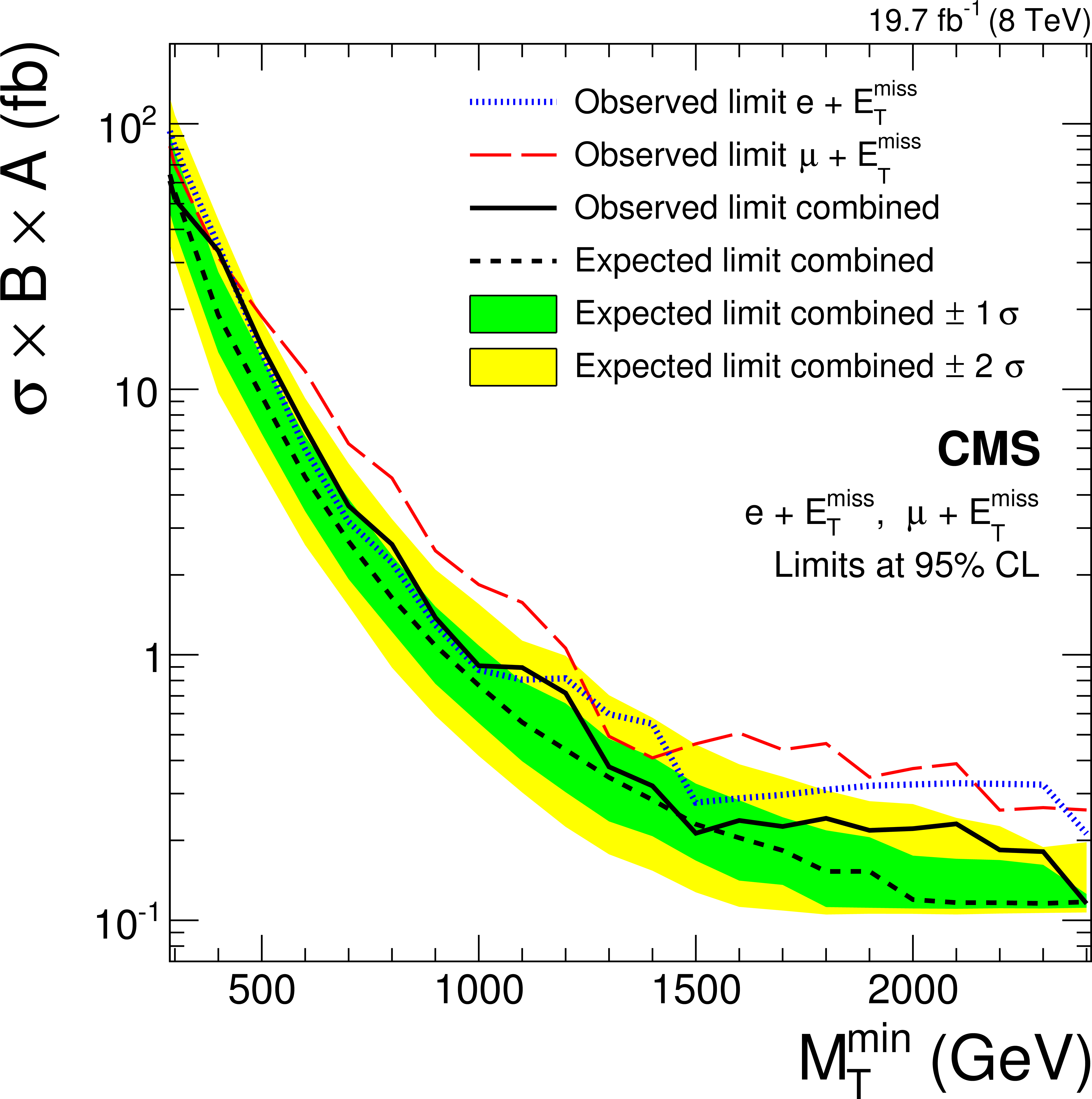
Figure 11:
Cross section upper limits at 95% CL on the effective cross section $\sigma ( {\mathrm {W}^\prime } )\mathcal {B}( {\mathrm {W}^\prime } \to \ell \nu )A$ above a threshold $ {M_\mathrm {T}^\mathrm {min}} $ for the combination of the electron and muon channels. Shown are the observed limits of the electron channel, muon channel, and the combination of both channels and the combined expected limit, together with the combined expected limit $1\sigma $ and $2\sigma $ intervals. Only detector acceptance is taken into account for the signal. The parameter $A$ describes the efficiency derived from the kinematic selection criteria and the $ {M_\mathrm {T}^\mathrm {min}} $ threshold. |
png pdf |
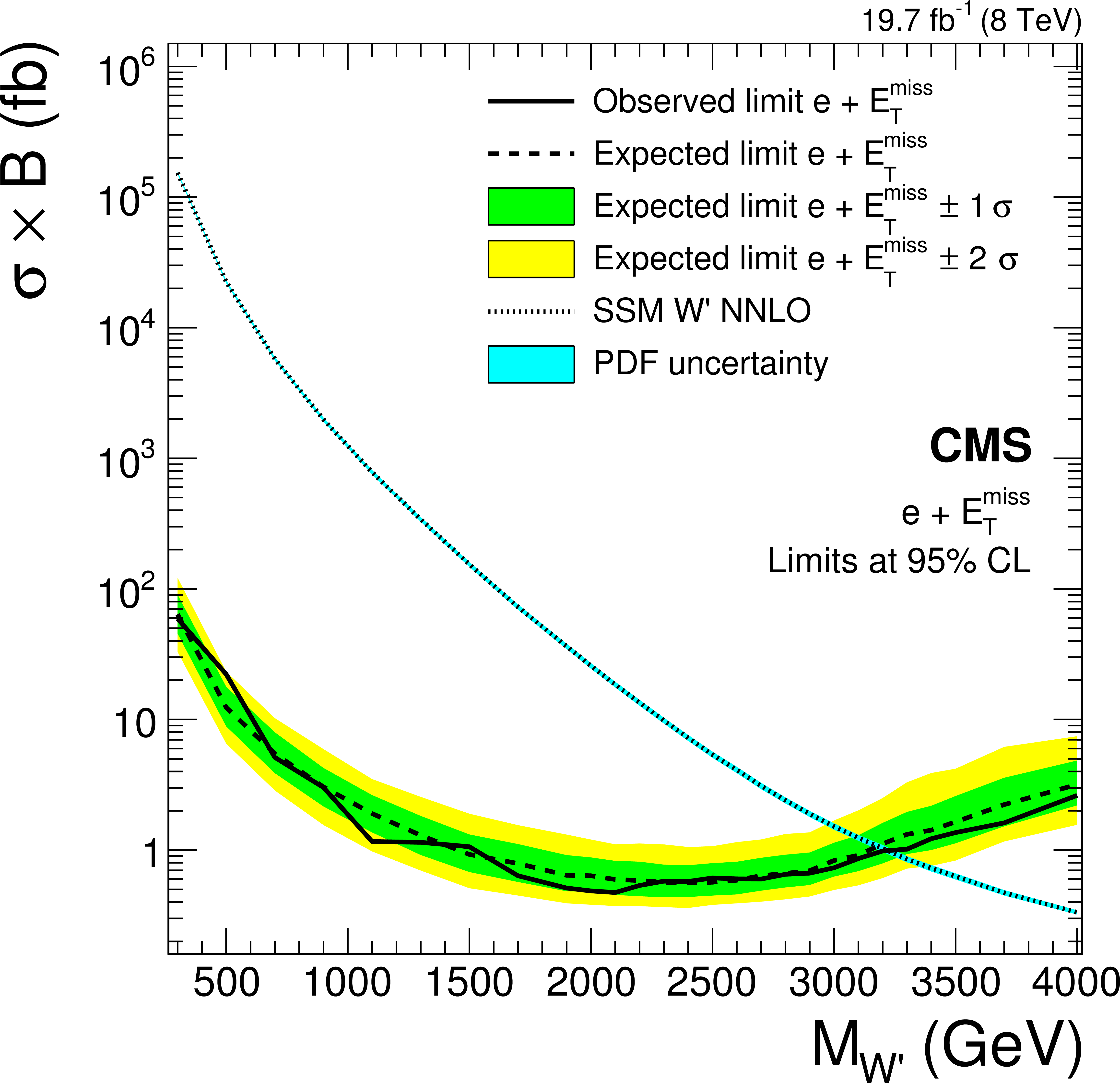
Figure 12-a:
Upper limits at 95% CL on $\sigma ( {\mathrm {W}^\prime } )\mathcal {B}( {\mathrm {W}^\prime } \to \ell \nu )$ with $\ell = {\mathrm {e}}$ (a) and $\ell = \mu $ (b). Shown are the theoretical cross section, the observed limit, the expected limit, and the expected limit $1\sigma $ and $2\sigma $ intervals. The theoretical cross section incorporates a mass-dependent NNLO K-factor. |
png pdf |
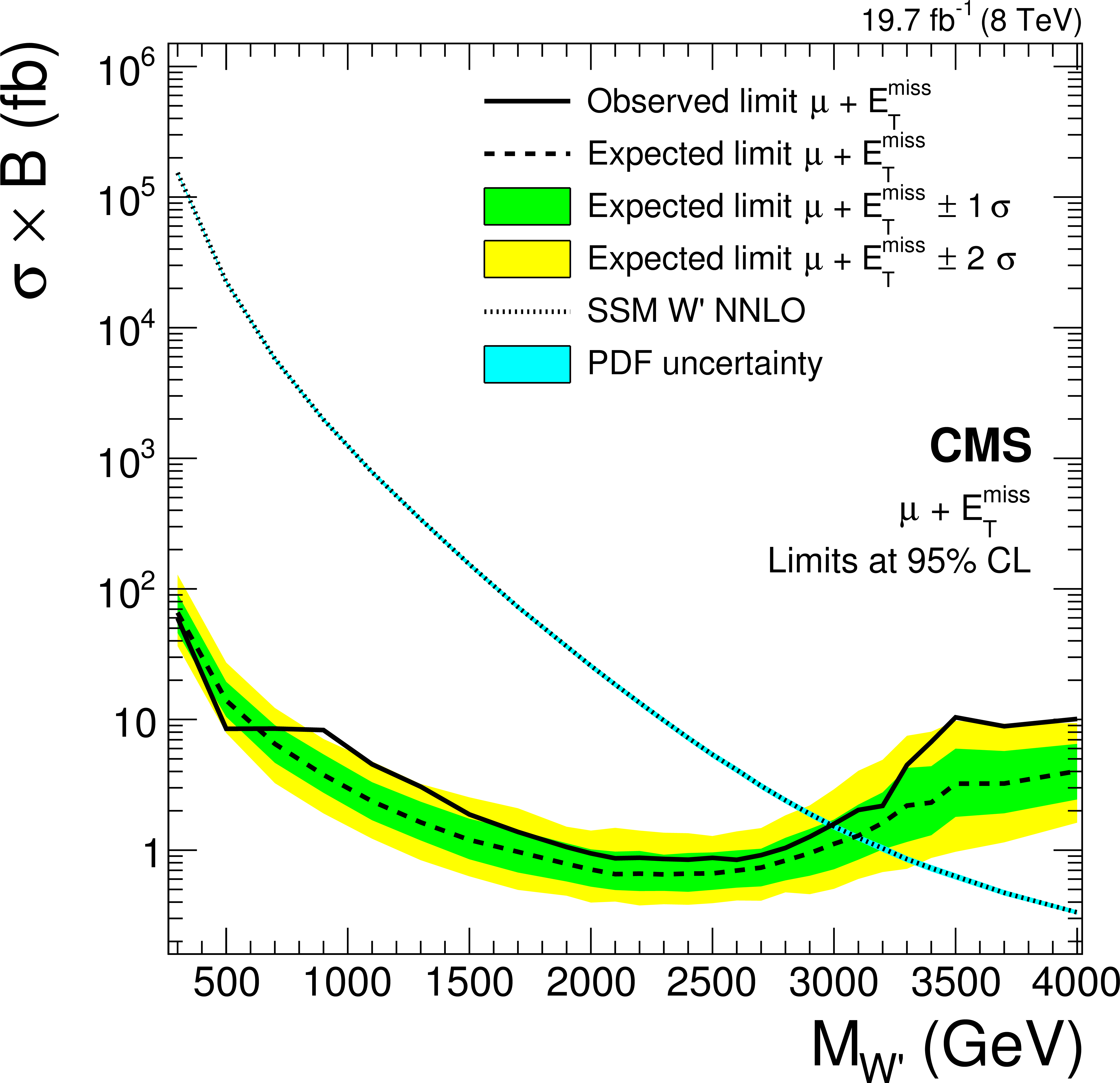
Figure 12-b:
Upper limits at 95% CL on $\sigma ( {\mathrm {W}^\prime } )\mathcal {B}( {\mathrm {W}^\prime } \to \ell \nu )$ with $\ell = {\mathrm {e}}$ (a) and $\ell = \mu $ (b). Shown are the theoretical cross section, the observed limit, the expected limit, and the expected limit $1\sigma $ and $2\sigma $ intervals. The theoretical cross section incorporates a mass-dependent NNLO K-factor. |

png pdf |
Figure 13:
Limits for heavy W' bosons for the electron and the muon channels, and for the two channels combined. Shown are the theoretical cross section for the SSM and two split-UED scenarios, the observed limit, the expected limit, and the expected limit $1\sigma $ and $2\sigma $ intervals. The theoretical cross sections incorporate a mass-dependent NNLO K-factor. The PDF uncertainties for the SSM are shown as a light blue band around the cross section curve. For the split-UED scenarios, the PDF uncertainties are expected to be small, similar to the uncertainty in the SSM scenario. |
png pdf |
Figure 14-a:
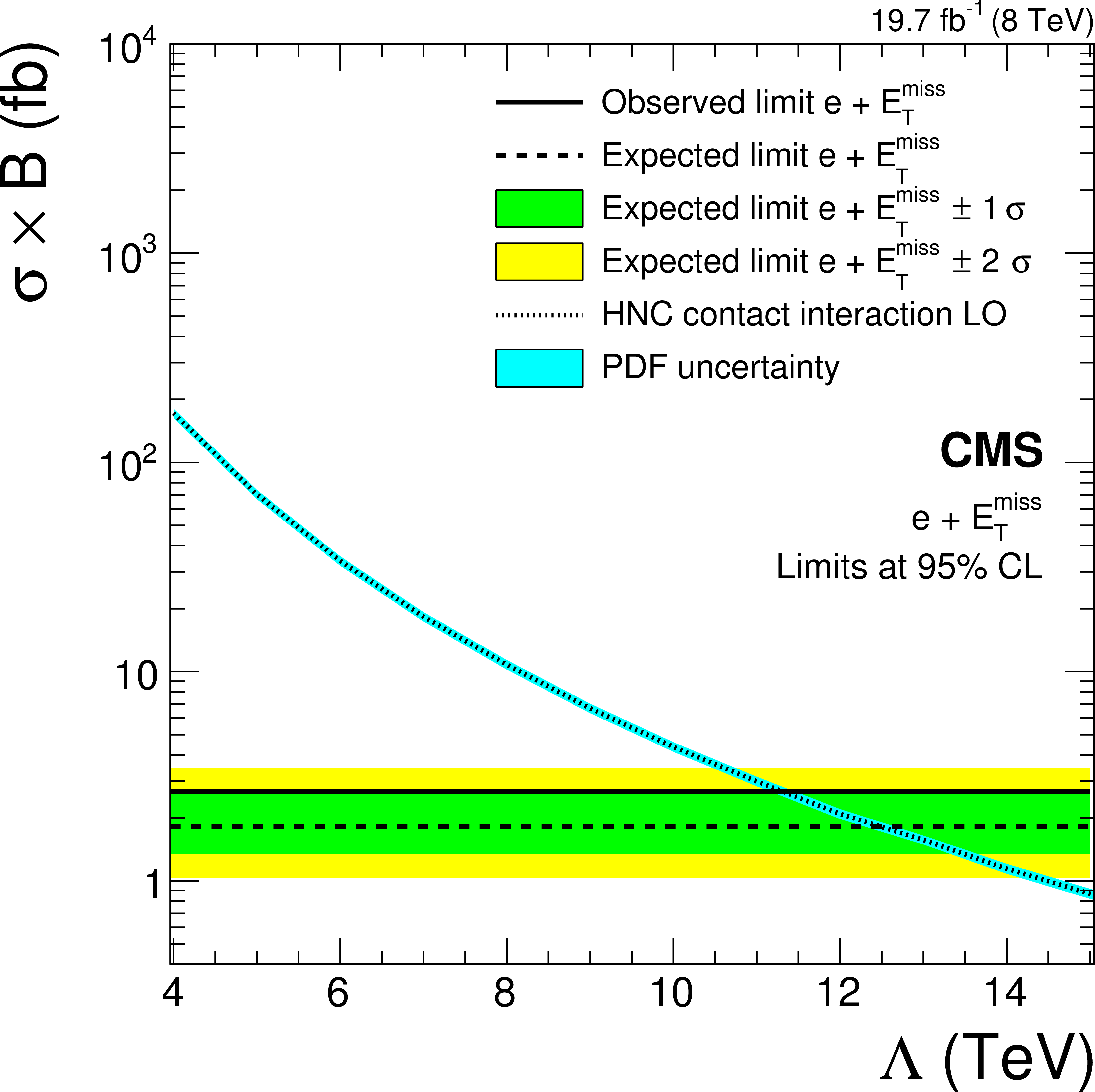
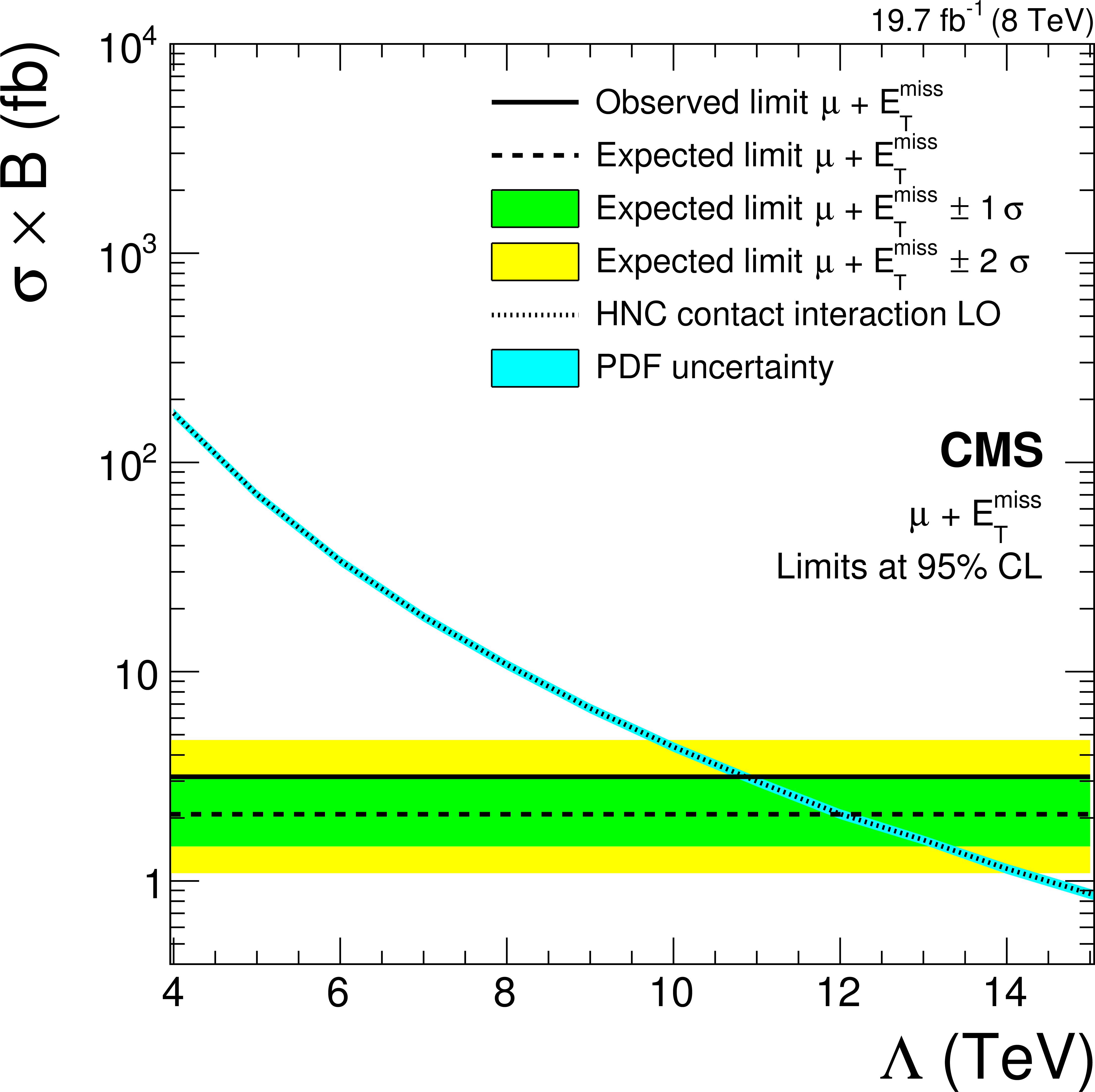
Upper limits at 95% CL on $\sigma \mathcal {B}( {\mathrm {p}} {\mathrm {p}}\to \ell \nu )$ with $\ell = {\mathrm {e}}$ (a) and $\ell = \mu $ (b) in terms of the contact interaction scale $\Lambda $ in the HNC-CI model. |
png pdf |
Figure 14-b:
Upper limits at 95% CL on $\sigma \mathcal {B}( {\mathrm {p}} {\mathrm {p}}\to \ell \nu )$ with $\ell = {\mathrm {e}}$ (a) and $\ell = \mu $ (b) in terms of the contact interaction scale $\Lambda $ in the HNC-CI model. |
png pdf |
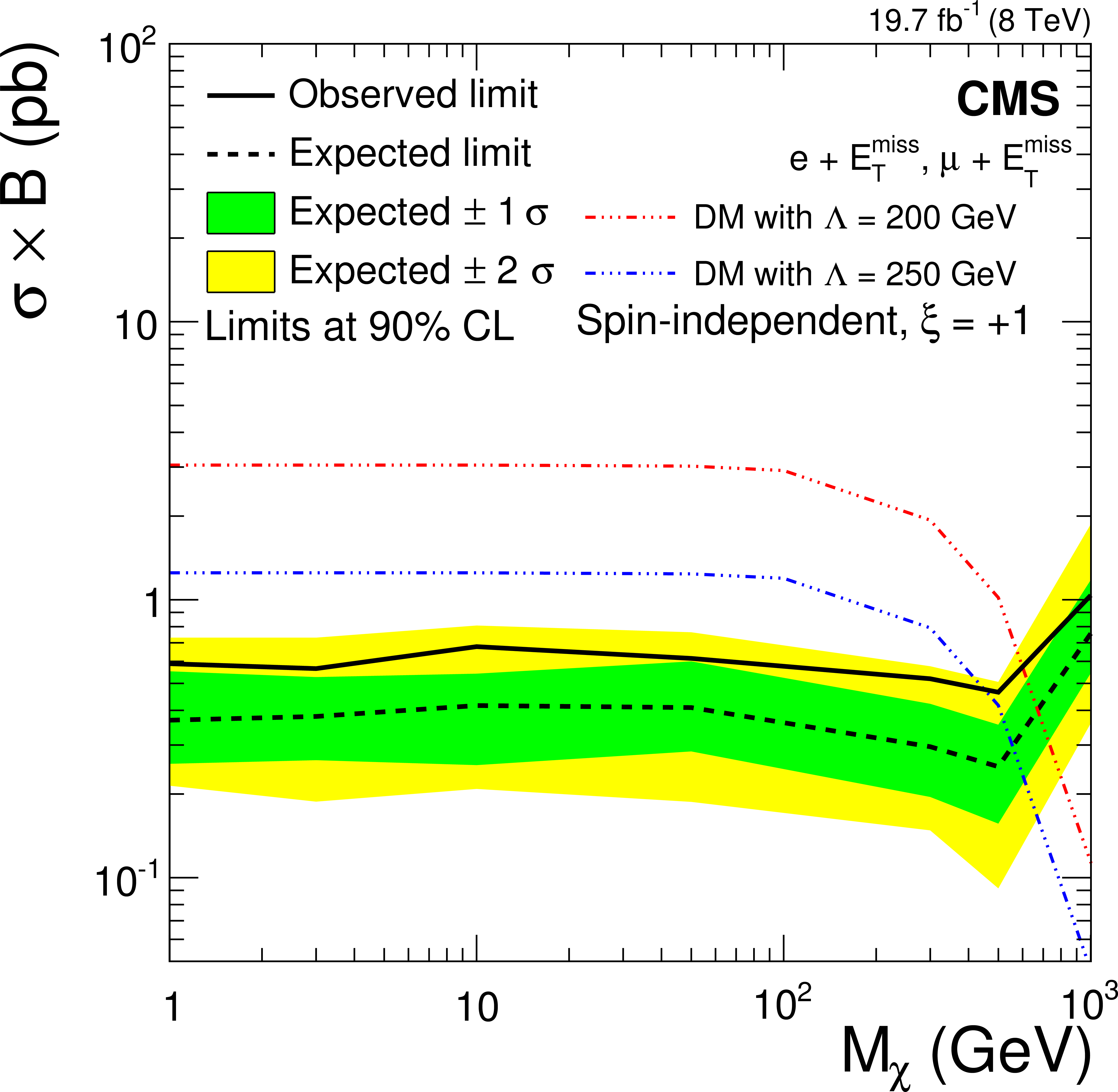
Figure 15-a:
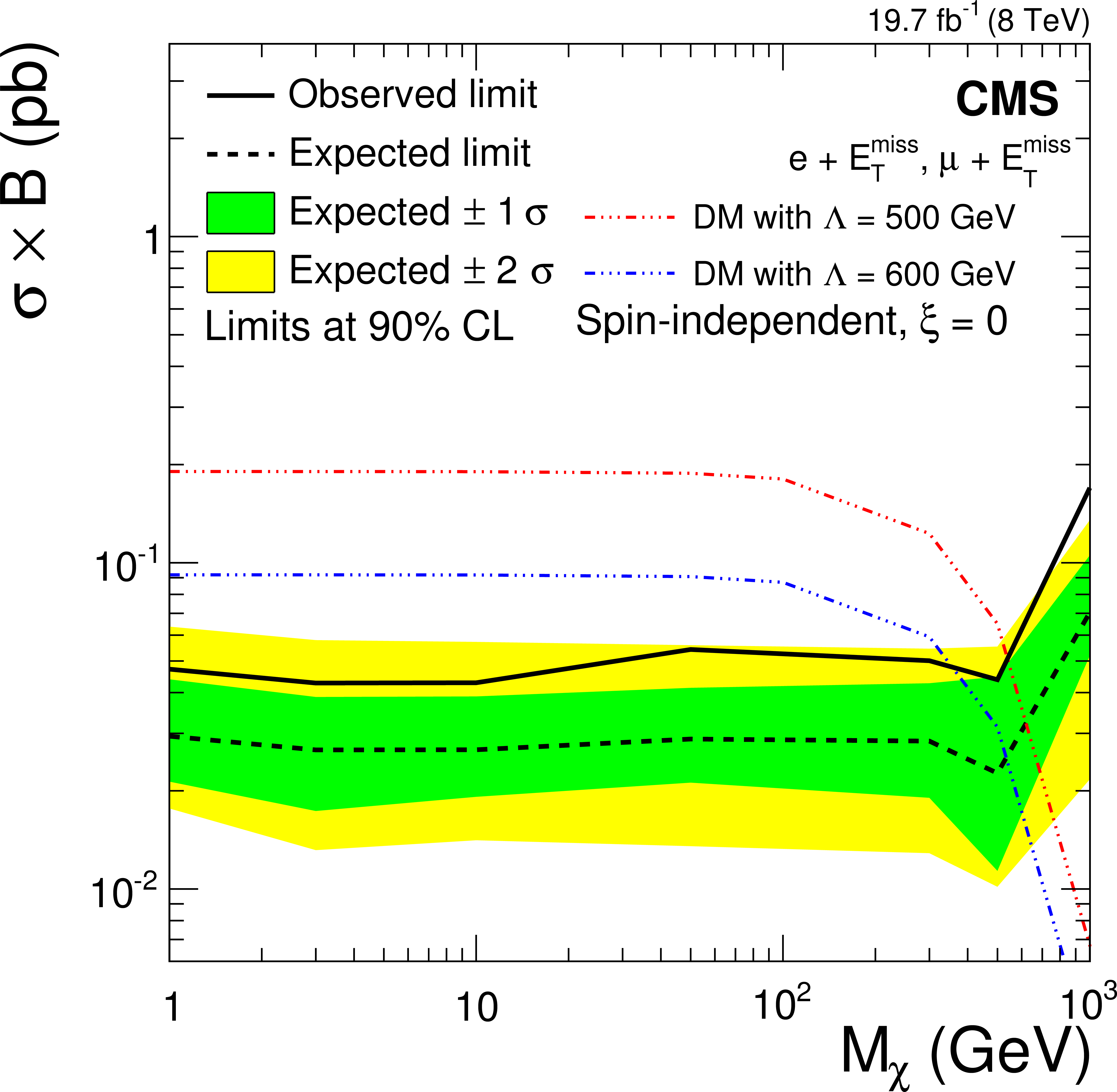
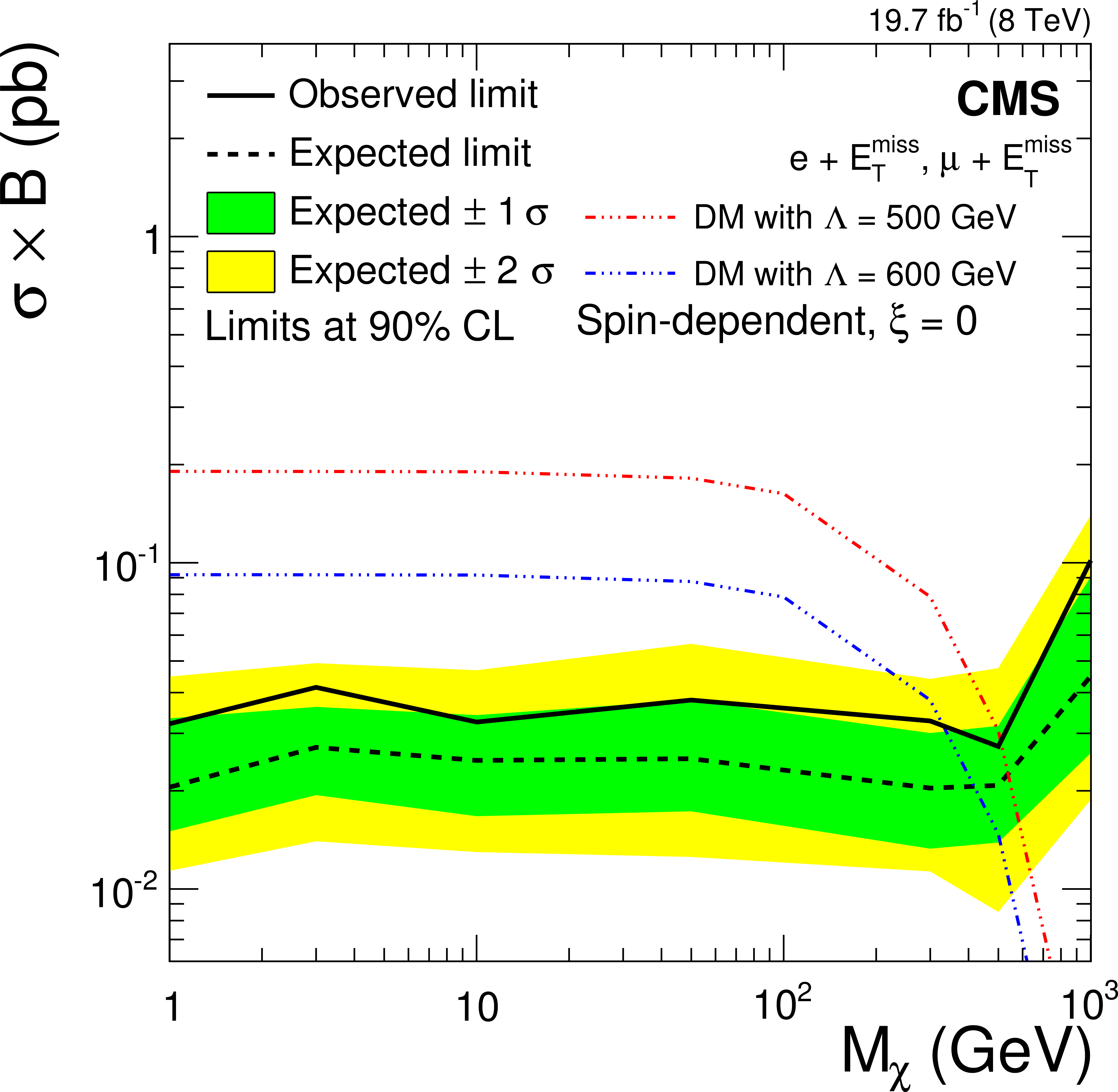
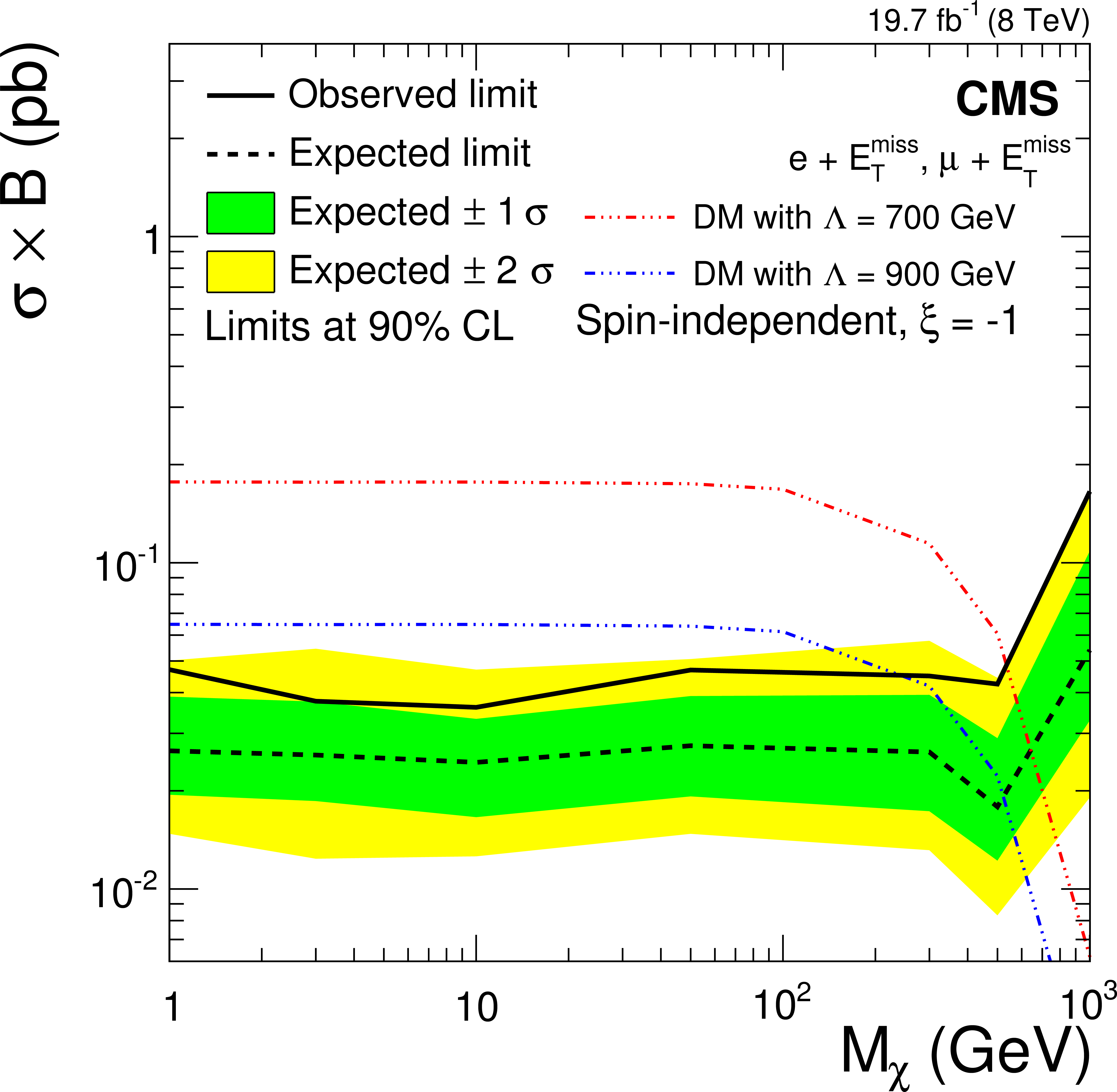
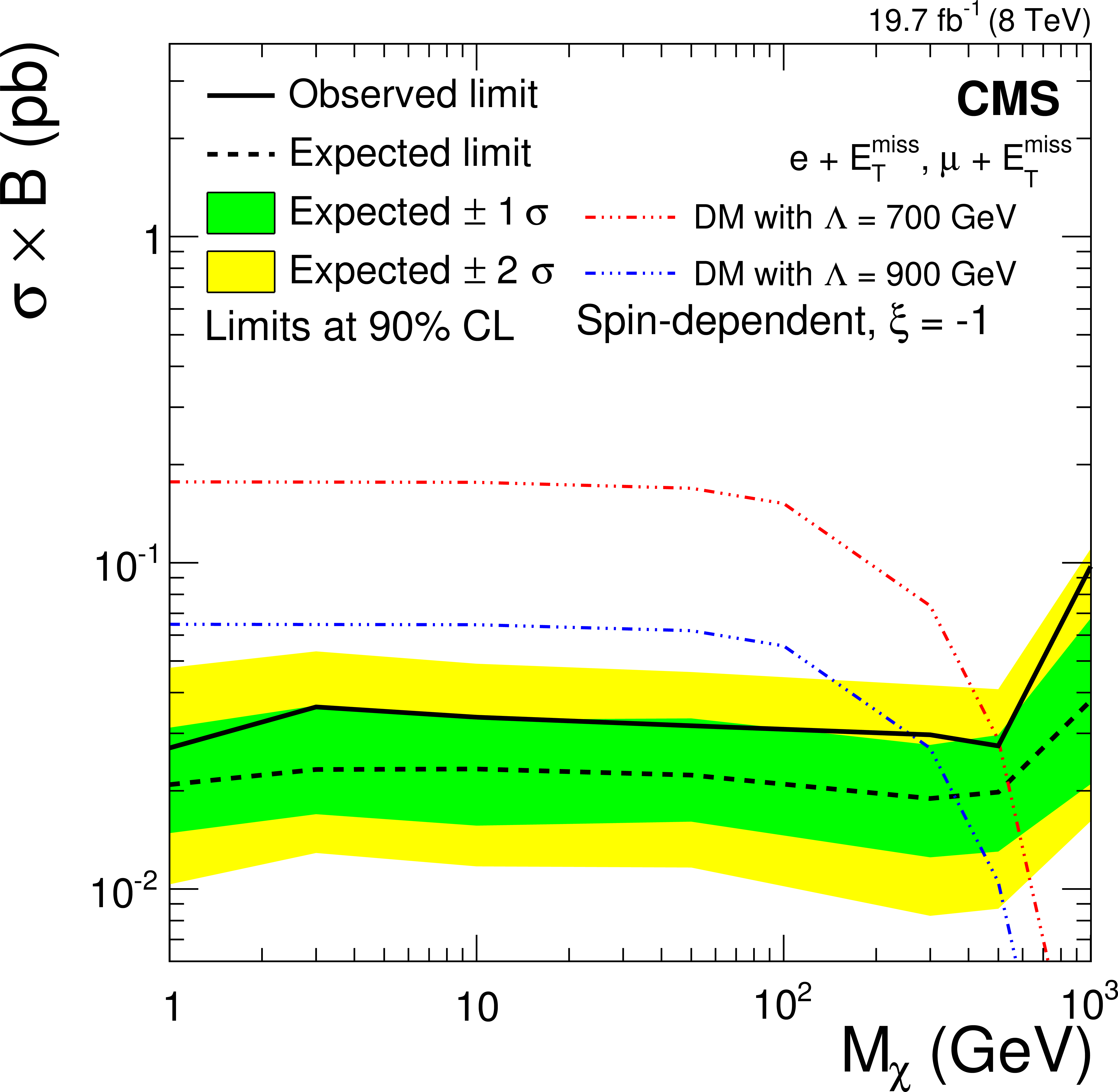
Upper limits on $\sigma \mathcal {B}( {\mathrm {p}} {\mathrm {p}}\to \chi \chi \ell \nu )$ for vector-like (spin-independent, a,c,e) and axial-vector-like (spin-dependent, b,d,f) couplings. Limits are calculated for the cases (from a,b to c,d to e,f) $\xi = +1,$ 0 and $-1$. Note the different vertical scales. |
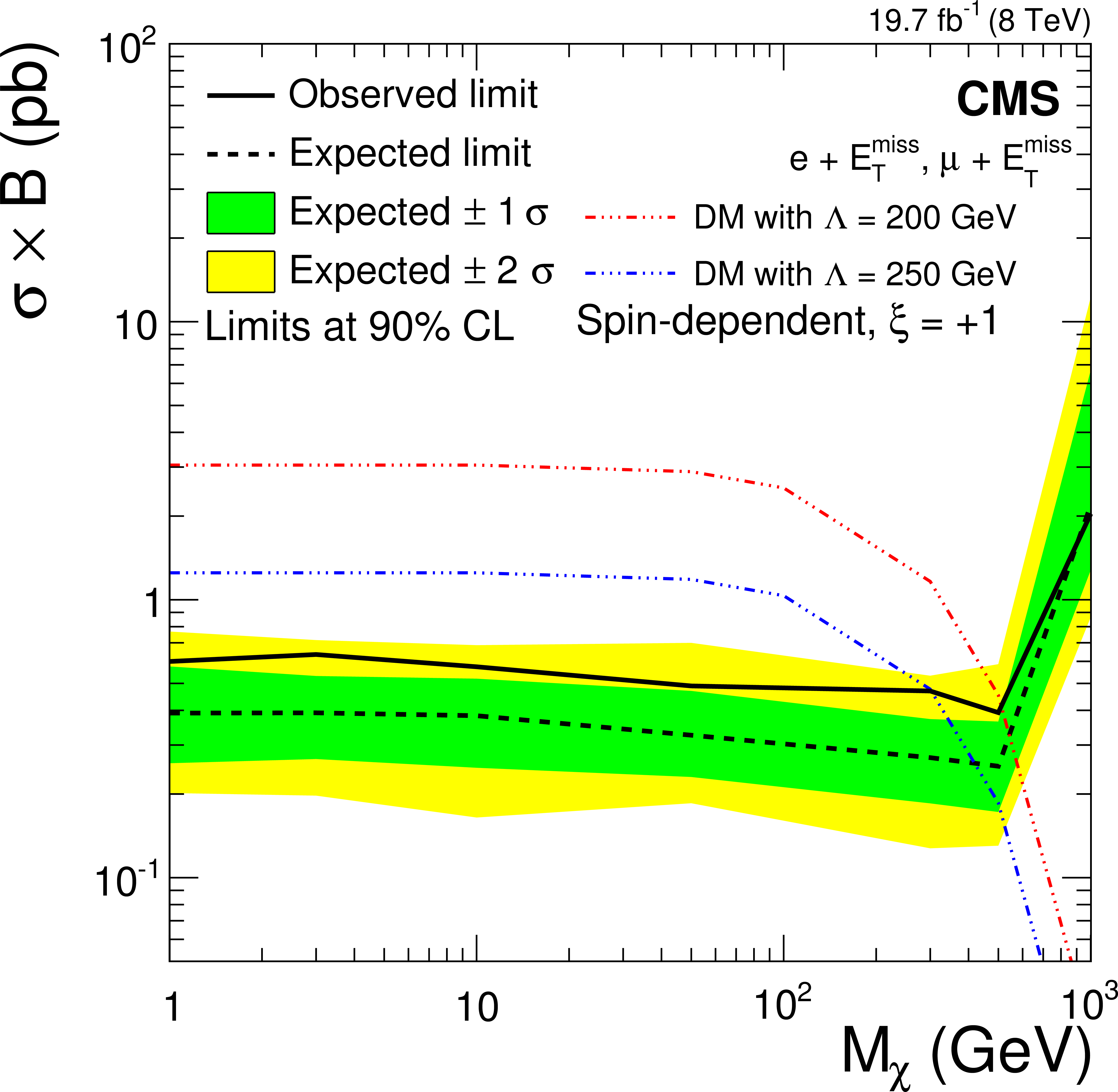
png pdf |
Figure 15-b:
Upper limits on $\sigma \mathcal {B}( {\mathrm {p}} {\mathrm {p}}\to \chi \chi \ell \nu )$ for vector-like (spin-independent, a,c,e) and axial-vector-like (spin-dependent, b,d,f) couplings. Limits are calculated for the cases (from a,b to c,d to e,f) $\xi = +1,$ 0 and $-1$. Note the different vertical scales. |
png pdf |
Figure 15-c:
Upper limits on $\sigma \mathcal {B}( {\mathrm {p}} {\mathrm {p}}\to \chi \chi \ell \nu )$ for vector-like (spin-independent, a,c,e) and axial-vector-like (spin-dependent, b,d,f) couplings. Limits are calculated for the cases (from a,b to c,d to e,f) $\xi = +1,$ 0 and $-1$. Note the different vertical scales. |
png pdf |
Figure 15-d:
Upper limits on $\sigma \mathcal {B}( {\mathrm {p}} {\mathrm {p}}\to \chi \chi \ell \nu )$ for vector-like (spin-independent, a,c,e) and axial-vector-like (spin-dependent, b,d,f) couplings. Limits are calculated for the cases (from a,b to c,d to e,f) $\xi = +1,$ 0 and $-1$. Note the different vertical scales. |
png pdf |
Figure 15-e:
Upper limits on $\sigma \mathcal {B}( {\mathrm {p}} {\mathrm {p}}\to \chi \chi \ell \nu )$ for vector-like (spin-independent, a,c,e) and axial-vector-like (spin-dependent, b,d,f) couplings. Limits are calculated for the cases (from a,b to c,d to e,f) $\xi = +1,$ 0 and $-1$. Note the different vertical scales. |
png pdf |
Figure 15-f:
Upper limits on $\sigma \mathcal {B}( {\mathrm {p}} {\mathrm {p}}\to \chi \chi \ell \nu )$ for vector-like (spin-independent, a,c,e) and axial-vector-like (spin-dependent, b,d,f) couplings. Limits are calculated for the cases (from a,b to c,d to e,f) $\xi = +1,$ 0 and $-1$. Note the different vertical scales. |

png pdf |
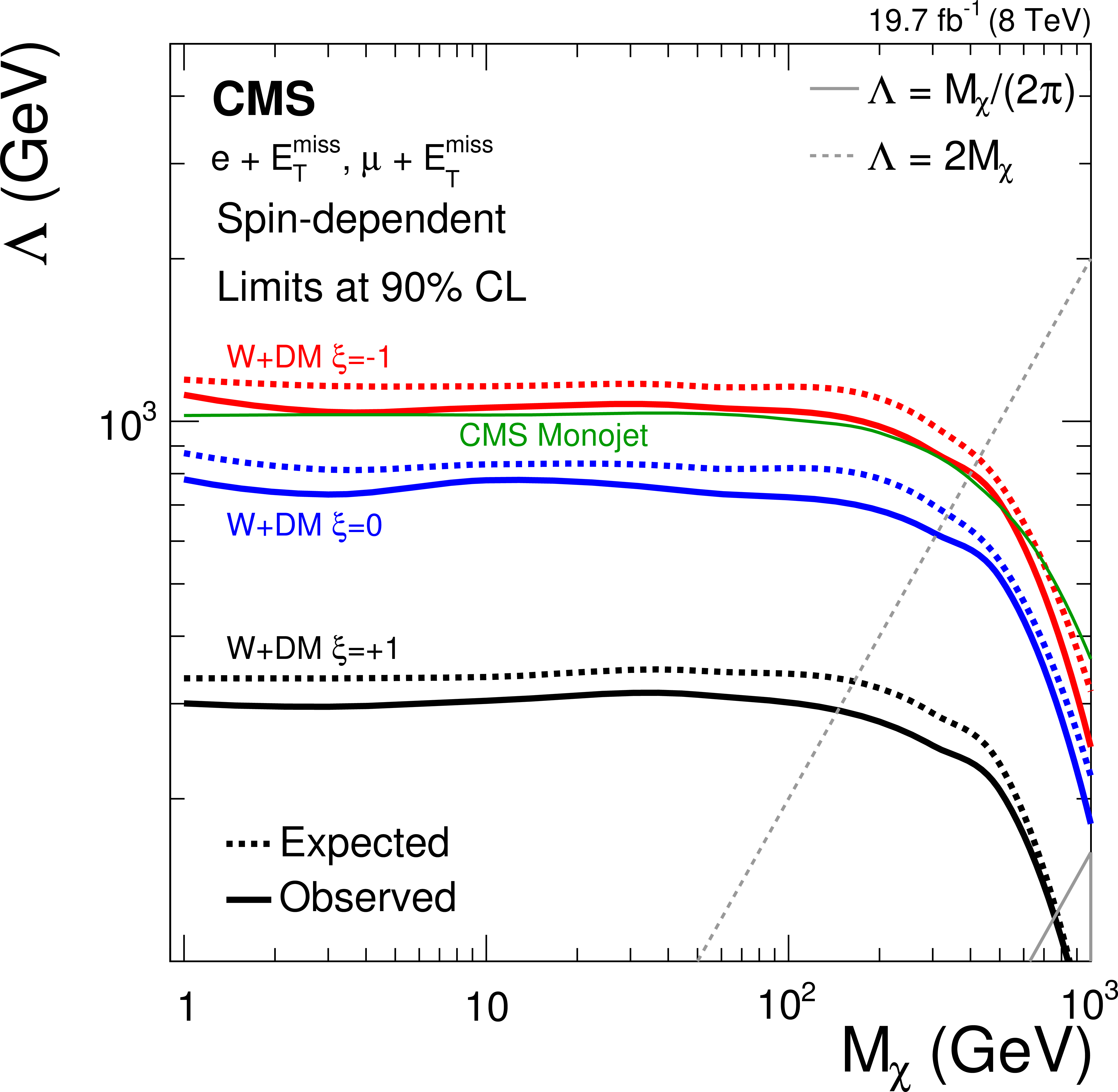
Figure 16-a:
Exclusion plane in $\Lambda $--${M_\chi } $, for the combination of the electron and muon channels. Vector-like (a) and axial-vector-like (b) couplings are shown. The two gray lines indicate where the coupling becomes non-perturbative and ($g_\mathrm {DM}$) is equal to 1, as described in Section 3.3. The green line shows the limit in the monojet final state (CMS-PAS-EXO-12-048), which is independent of $\xi $ for the limit on $\Lambda $. |
png pdf |
Figure 16-b:
Exclusion plane in $\Lambda $--${M_\chi } $, for the combination of the electron and muon channels. Vector-like (a) and axial-vector-like (b) couplings are shown. The two gray lines indicate where the coupling becomes non-perturbative and ($g_\mathrm {DM}$) is equal to 1, as described in Section 3.3. The green line shows the limit in the monojet final state (CMS-PAS-EXO-12-048), which is independent of $\xi $ for the limit on $\Lambda $. |
png pdf |
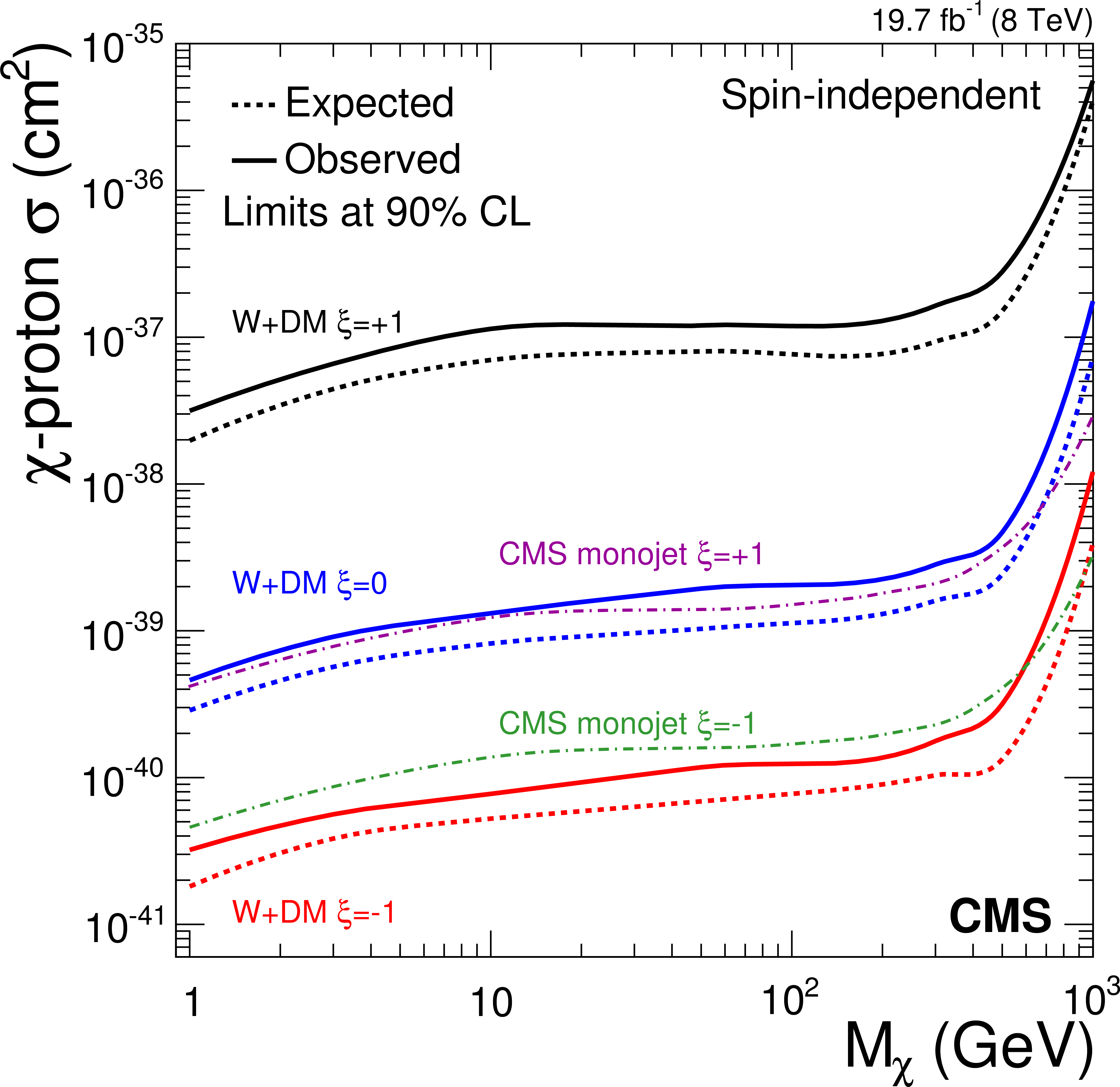
Figure 17-a:
Excluded proton-dark matter cross section for vector-like (a) and axial-vector-like (b) couplings, for the combination of the electron and muon channels. For comparison the result from the monojet DM search (CMS-PAS-EXO-12-048) is also shown. |
png pdf |
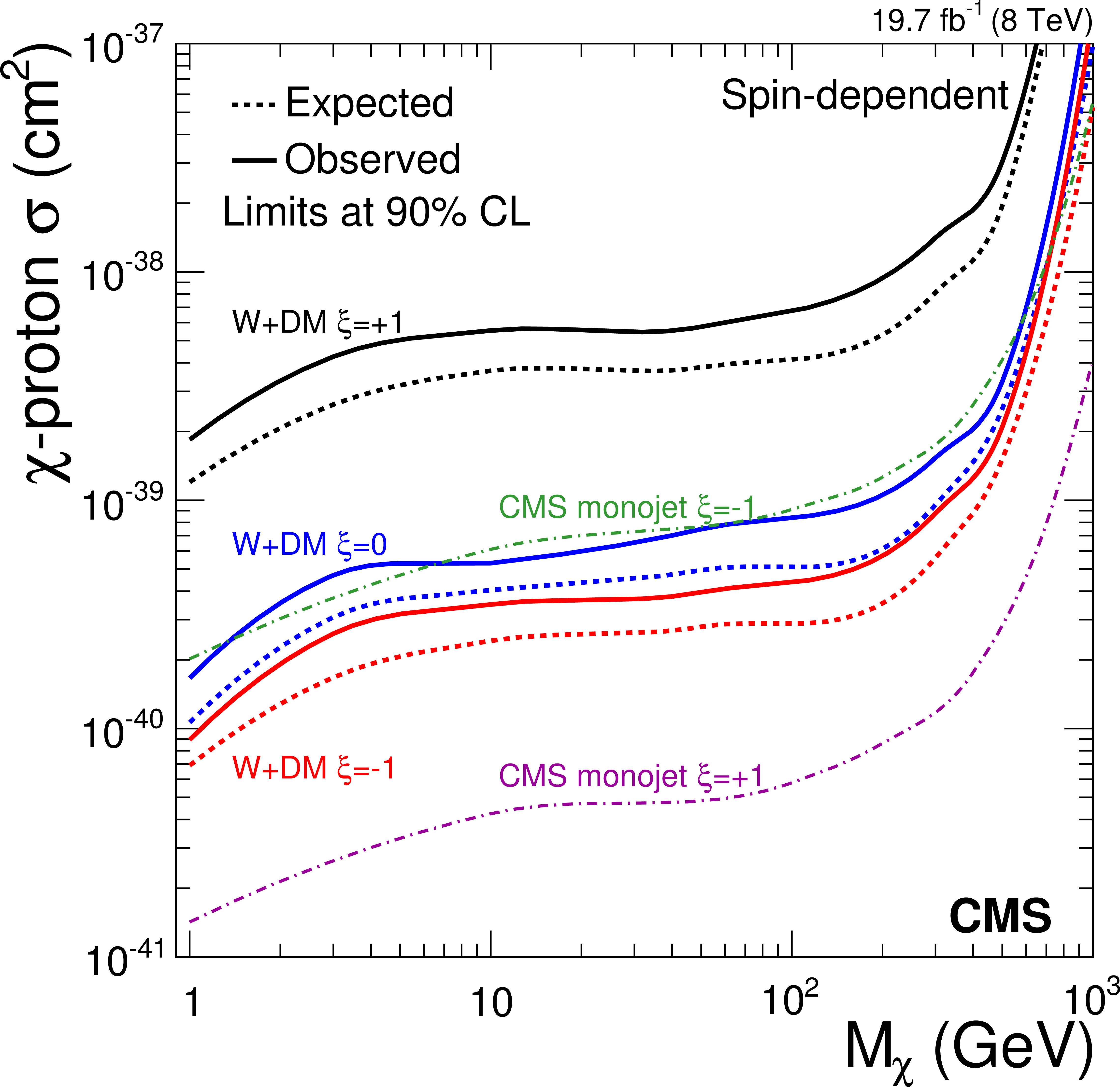
Figure 17-b:
Excluded proton-dark matter cross section for vector-like (a) and axial-vector-like (b) couplings, for the combination of the electron and muon channels. For comparison the result from the monojet DM search (CMS-PAS-EXO-12-048) is also shown. |
png pdf |
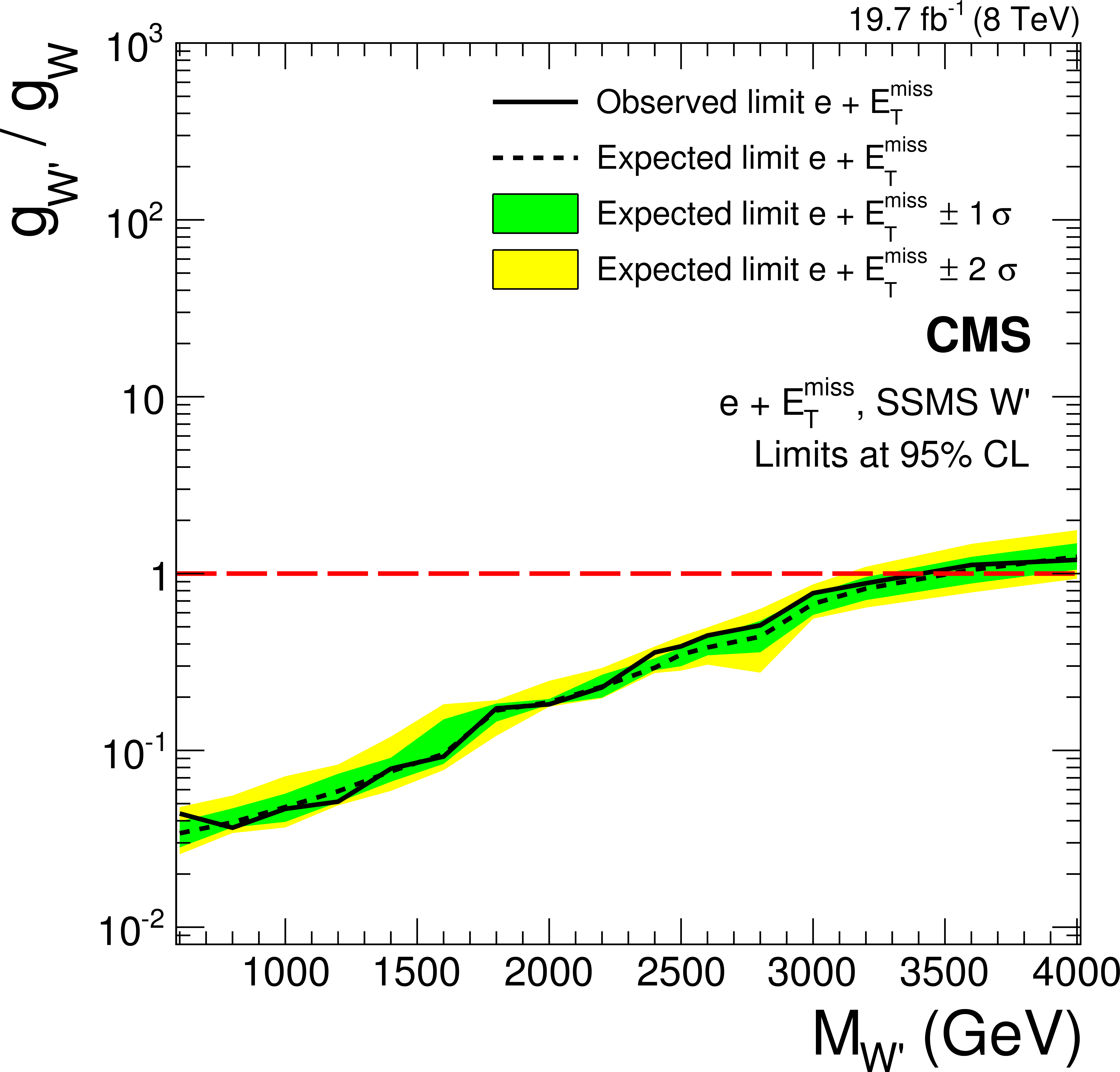
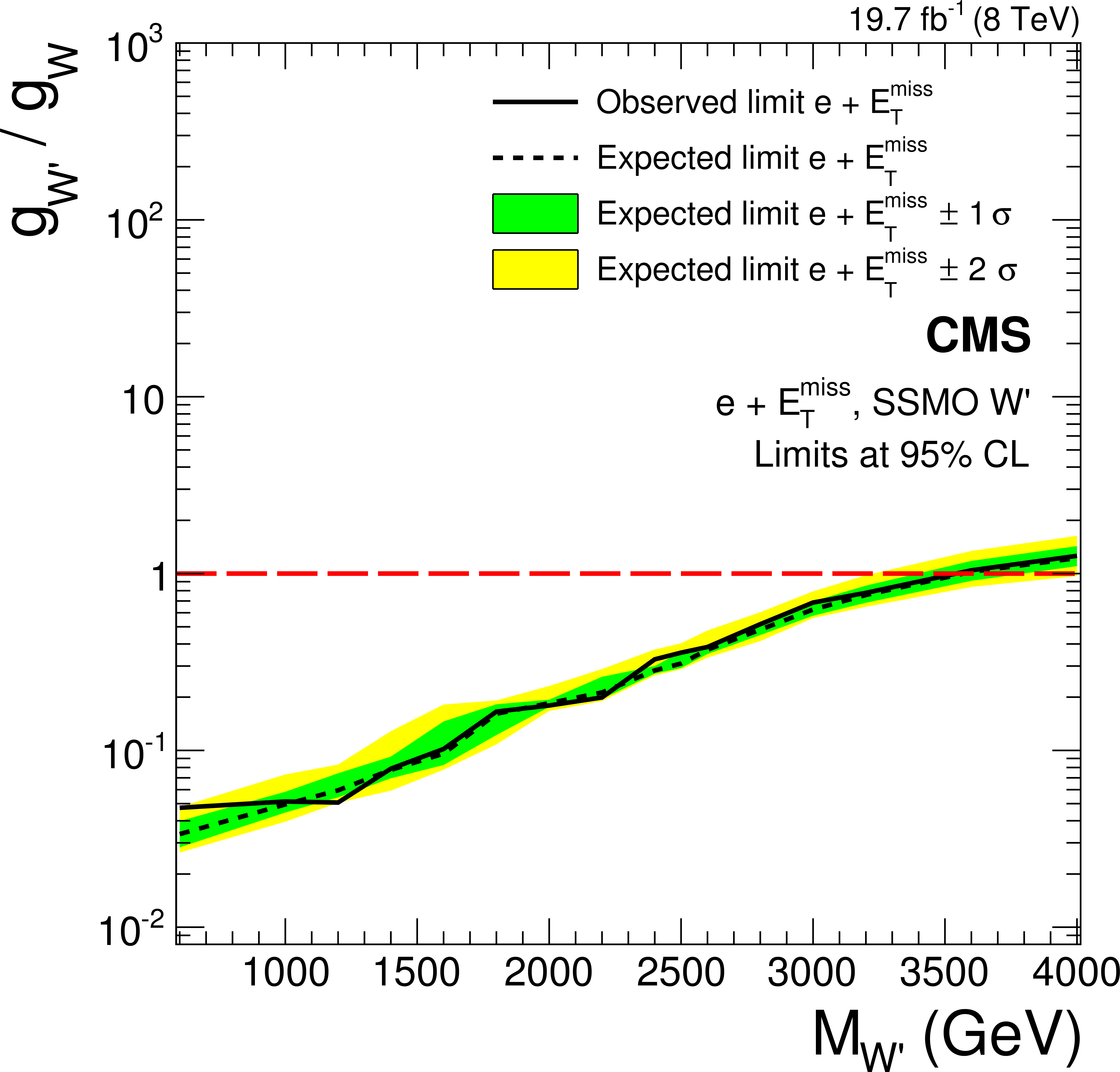
Figure 18-a:
Limits on the coupling $g_{ {\mathrm {W}^\prime } }$ in terms of the SM coupling $g_{ {\mathrm {W}}}$ in the electron (a,b) and muon (c,d) channels, and their combination (e,f). Limits for the SSMS model are displayed in a,c,e, those for the SSMO model in b,d,f. |
png pdf |
Figure 18-b:
Limits on the coupling $g_{ {\mathrm {W}^\prime } }$ in terms of the SM coupling $g_{ {\mathrm {W}}}$ in the electron (a,b) and muon (c,d) channels, and their combination (e,f). Limits for the SSMS model are displayed in a,c,e, those for the SSMO model in b,d,f. |
png pdf |
Figure 18-c:
Limits on the coupling $g_{ {\mathrm {W}^\prime } }$ in terms of the SM coupling $g_{ {\mathrm {W}}}$ in the electron (a,b) and muon (c,d) channels, and their combination (e,f). Limits for the SSMS model are displayed in a,c,e, those for the SSMO model in b,d,f. |

png pdf |
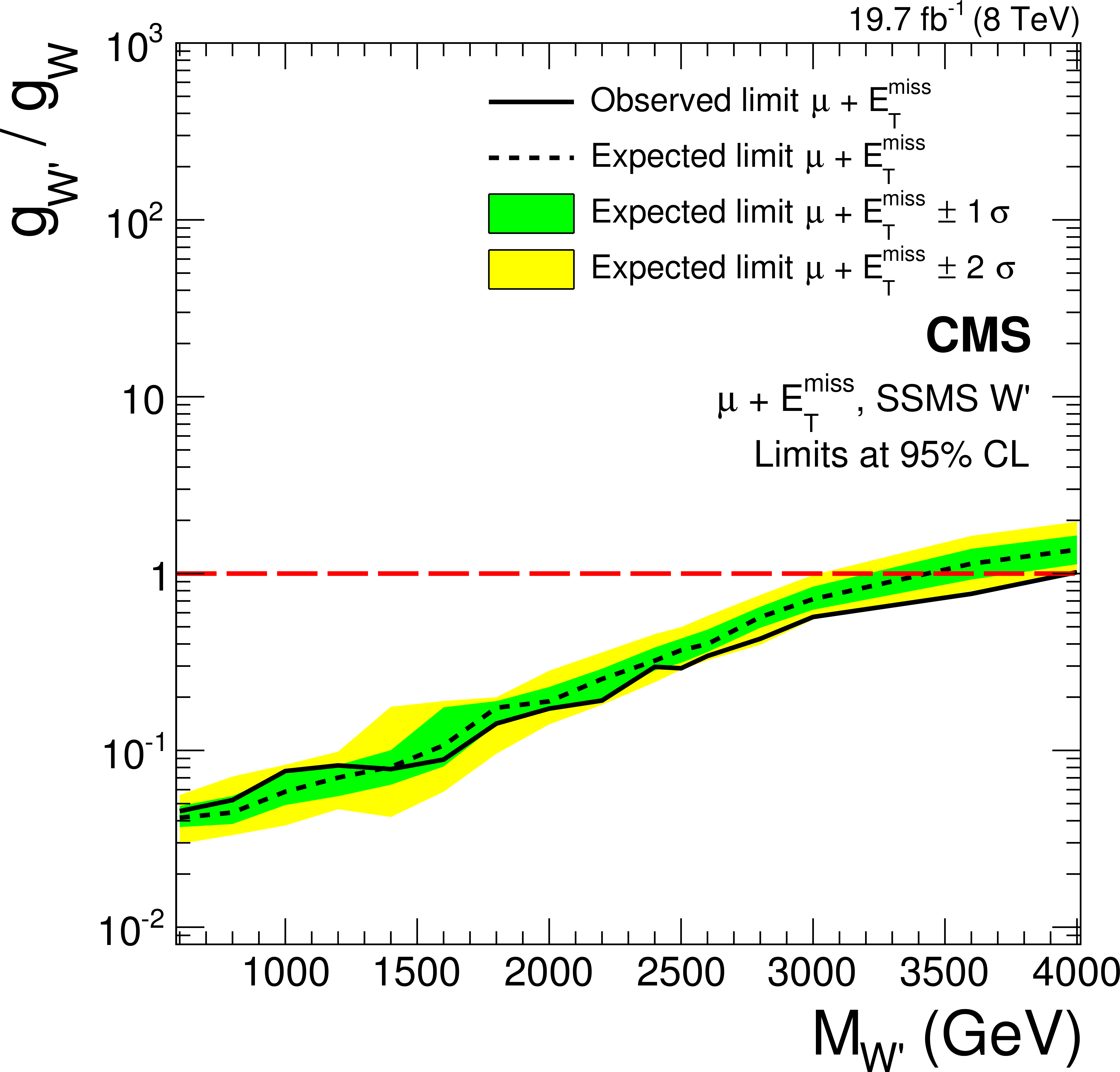
Figure 18-d:
Limits on the coupling $g_{ {\mathrm {W}^\prime } }$ in terms of the SM coupling $g_{ {\mathrm {W}}}$ in the electron (a,b) and muon (c,d) channels, and their combination (e,f). Limits for the SSMS model are displayed in a,c,e, those for the SSMO model in b,d,f. |
png pdf |
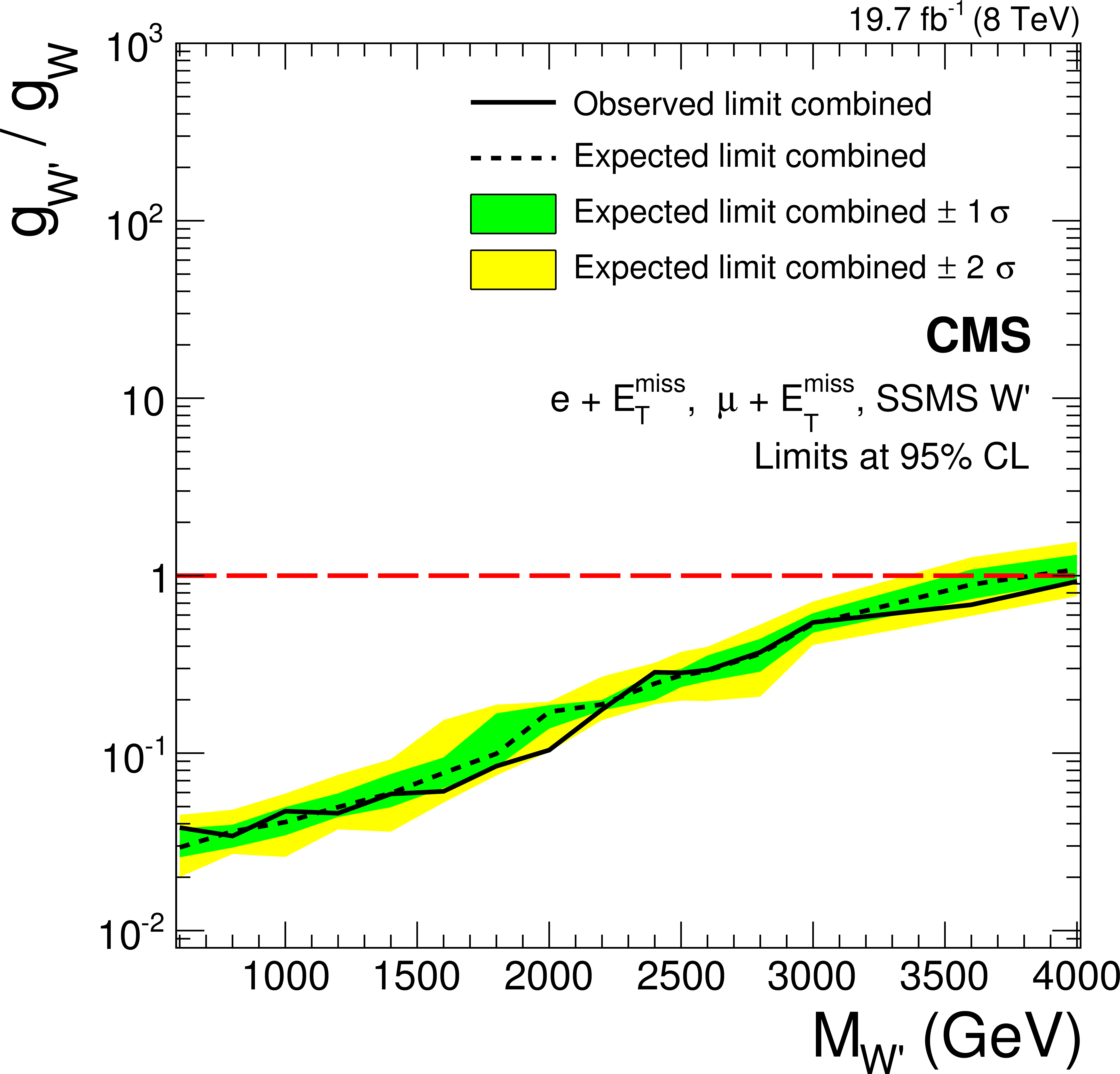
Figure 18-e:
Limits on the coupling $g_{ {\mathrm {W}^\prime } }$ in terms of the SM coupling $g_{ {\mathrm {W}}}$ in the electron (a,b) and muon (c,d) channels, and their combination (e,f). Limits for the SSMS model are displayed in a,c,e, those for the SSMO model in b,d,f. |

png pdf |
Figure 18-f:
Limits on the coupling $g_{ {\mathrm {W}^\prime } }$ in terms of the SM coupling $g_{ {\mathrm {W}}}$ in the electron (a,b) and muon (c,d) channels, and their combination (e,f). Limits for the SSMS model are displayed in a,c,e, those for the SSMO model in b,d,f. |
png pdf |
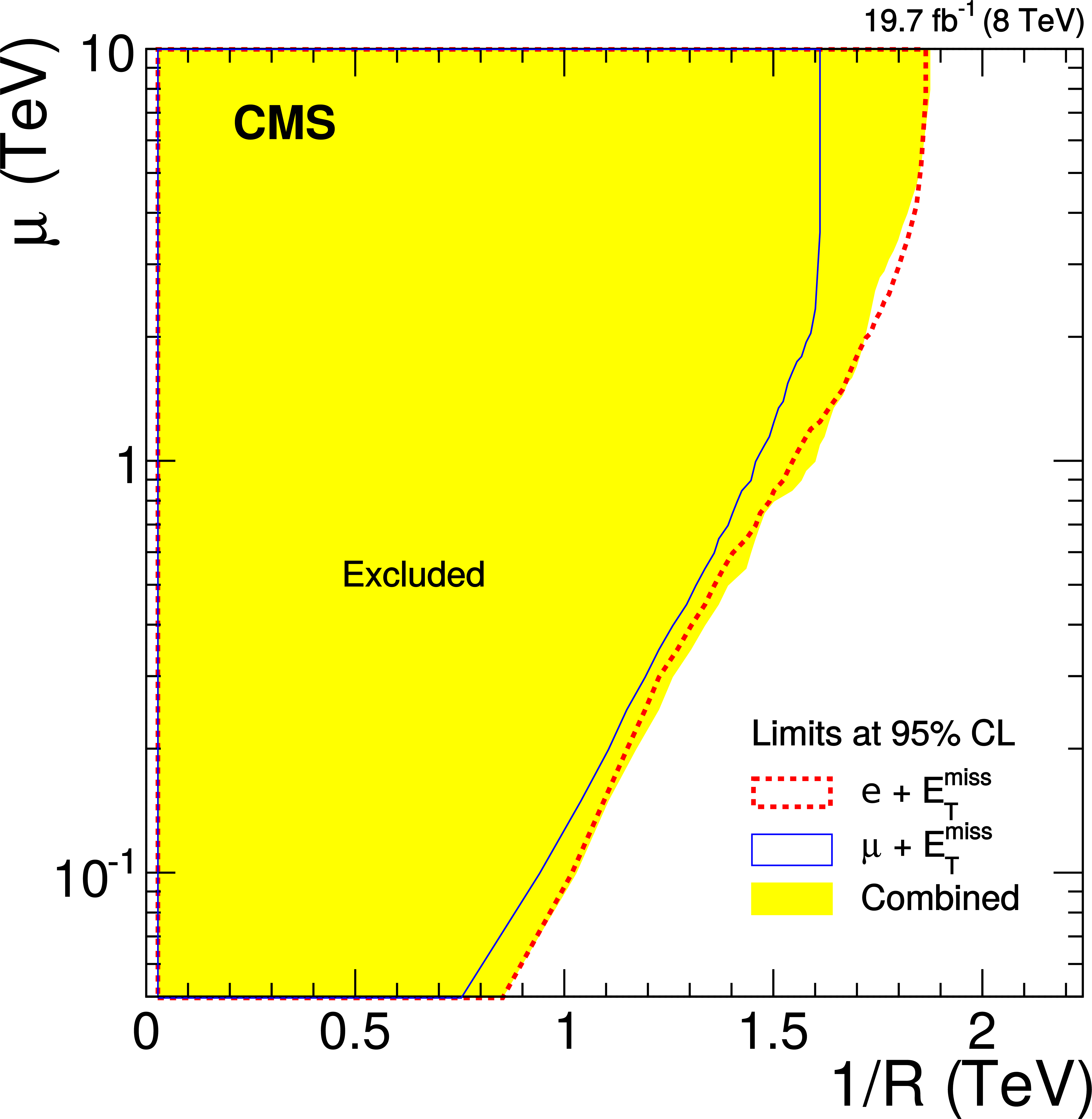
Figure 19:
Limits on the split-UED parameters $\mu $ and $1/R$, derived from the W'-boson mass limits, taking into account the corresponding width of the $ {\mathrm {W}^\mathrm {(2)}_\mathrm {KK}} $ boson. |
png pdf |
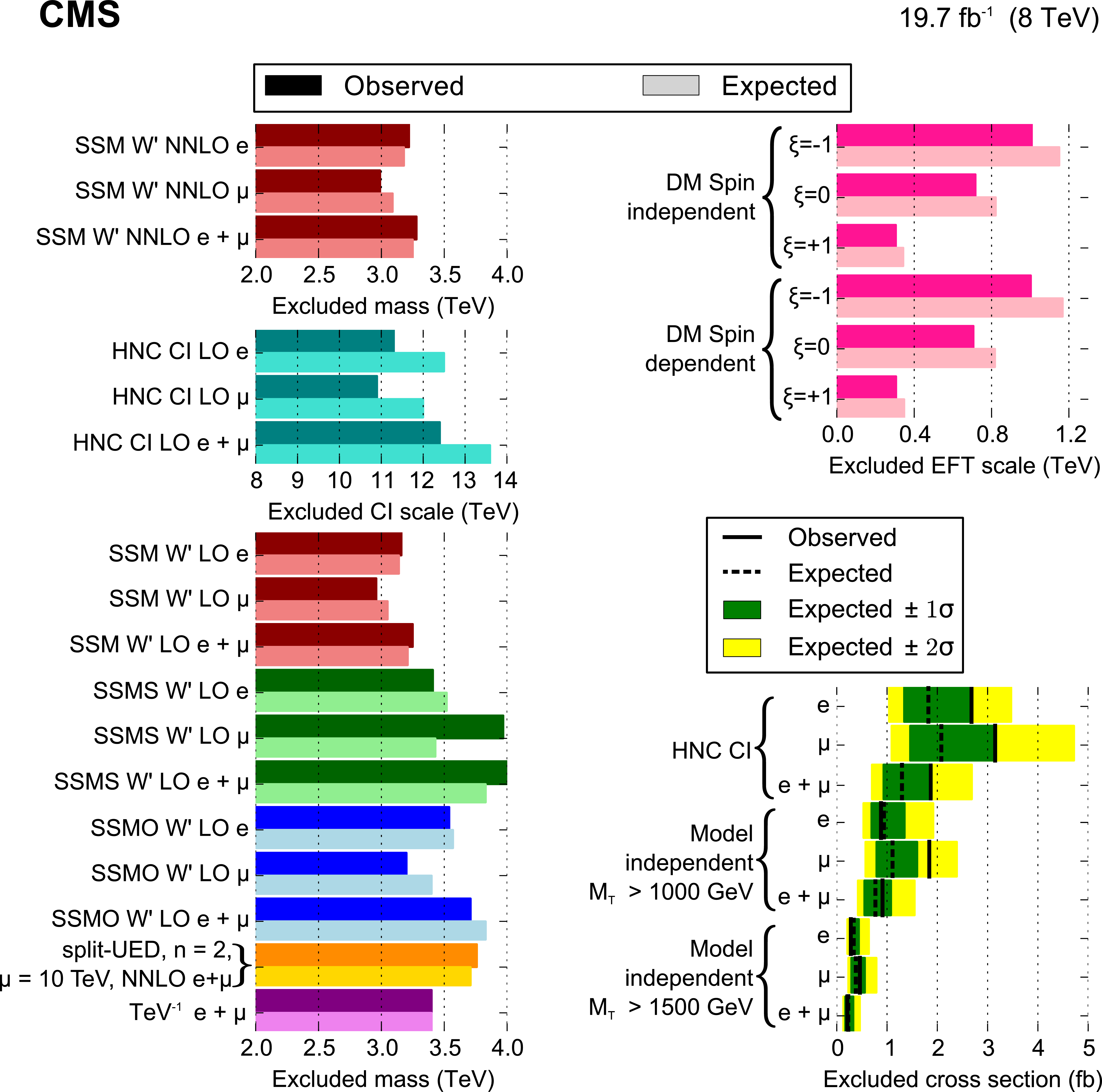
Figure 20:
Summary of all exclusion limits in the electron and muon channels, and for their combinations. No interference of W' and W bosons is considered in the interpretation labeled as SSM while it is taken into account in the SSMS and SSMO models. For the HNC contact interaction, the compositeness scale $\Lambda $ is probed. In the upper rows of the right column, the EFT limits are shown for the DM interpretations in term of $\Lambda $ for small dark matter masses $M_\chi <$ 100 GeV. The reinterpretation in terms of additional extra dimensions is provided in the context of split-UED, given for a bulk mass parameter $\mu =$ 10 TeV, and in the TeV$^{-1}$ model. |
| Summary |
|
A search for physics beyond the standard model, based on events with a final state contain- ing a charged lepton (electron or muon) and significant missing transverse energy, has been performed, using proton-proton collision data at $\sqrt{s} = $ 8 TeV, corresponding to an integrated luminosity of 19.7 fb$^{-1}$. No significant deviation from the standard model expectation has been observed in the transverse mass distribution.
A model-independent upper limit at 95% CL on the cross section times branching fraction of additional contributions has been established, ranging from 100 to 0.1 fb over an $M_{\mathrm{T}}$ range of 300 GeV to 2.5 TeV, respectively. The results have been interpreted in the context of various models, as summarized below. An SSM W′ boson that does not interfere with the W boson has been excluded at 95% CL for W′-boson masses up to 3.22 (2.99) TeV for the electron (muon) channel, where the expected limit is 3.18 (3.06) TeV. When combining both channels, the limit improves to 3.28 TeV. Lower mass limits in either channel are implicit due to trigger thresholds. An interpretation in terms of a four-fermion contact interaction yields a limit for the compositeness energy scale $\Lambda$ of 11.3 TeV in the electron channel, 10.9 TeV in the muon channel, and 12.4 TeV for their combination. Assuming the production of a pair of dark matter particles along with a recoiling W boson that subsequently decays leptonically, the results have been reinterpreted in terms of an effective dark matter theory. The effective scale is excluded below 0.3 to 1 TeV, depending on model parameters. This is particularly interesting for low masses of dark matter particles, where the sensitivity of direct searches is poor. Building upon earlier versions of this analysis [24], the expected impact of W-W′ interference on the shape of the W boson $M_{\mathrm{T}}$ distribution is fully taken into account. Along with the shape, the expected cross section varies, making possible the setting of limits for models with both destructive (SSMS) and constructive (SSMO) interference. The lower limit on the W′-boson mass is 3.41 (3.97) TeV in the electron (muon) channels for the SSMS and 3.54 (3.22) TeV for the SSMO. For the first time, limits in terms of generalized lepton couplings are given. An interpretation of the search results has been made in a specific framework of universal extra dimensions where bulk fermions propagate in the one additional dimension. The second Kaluza–Klein excitation W(2) has been excluded for masses below 1.74 TeV, assuming a bulk KK mass parameter $\mu$ of 0.05 TeV, or for masses below 3.71 TeV, for $\mu =$ 10 TeV. In an alternative model in which only SM gauge bosons propagate in a compactified extra dimension (TeV$^{-1}$ model), a lower bound on the size of the compactified dimension, MC , has been set at 3.40 TeV. Study of the mono-lepton channel provides a powerful tool to probe for beyond the standard model physics. All the results of this search are summarized in Fig. 20, including the expected and observed limits. Fig. 20 is structured by theories and the related model parameters (particle mass, compositeness scale $\Lambda$ or dark matter effective field scale $\Lambda$) as given. The three representative signal examples (SSM W′, contact interaction and dark matter) are shown in the upper figure section. Limits for specific models along with the model independent cross section limit are given in the lower part of the figure. |
|
|
Compact Muon Solenoid LHC, CERN |
|

|

|

|

|

|