

Compact Muon Solenoid
LHC, CERN
| CMS-EXO-14-009 ; CERN-PH-EP-2015-096 | ||
| Search for a massive resonance decaying into a Higgs boson and a W or Z boson in hadronic final states in proton-proton collisions at $\sqrt{s}= $ 8 TeV | ||
| CMS Collaboration | ||
| 4 June 2015 | ||
| J. High Energy Phys. 02 (2016) 145 | ||
| Abstract: A search for a massive resonance decaying into a standard-model-like Higgs boson (H) and a W or Z boson is reported. The analysis is performed on a data sample corresponding to an integrated luminosity of 19.7 fb$^{-1}$, collected in proton-proton collisions at a centre-of-mass energy of 8 TeV with the CMS detector at the LHC. Signal events, in which the decay products of Higgs, W, or Z bosons at high Lorentz boost are contained within single reconstructed jets, are identified using jet substructure techniques, including the tagging of b hadrons. This is the first search for heavy resonances decaying into HW or HZ resulting in an all-jet final state, as well as the first application of jet substructure techniques to identify $\mathrm{ H \to W W^* \to 4q}$ decays at high Lorentz boost. No significant signal is observed and limits are set at 95% confidence level on the production cross section of W' and Z' in a model with mass-degenerate charged and neutral spin-1 resonances. Resonance masses are excluded for W' in the interval [1.0, 1.6] TeV, for Z' in the intervals [1.0, 1.1] and [1.3,1.5] TeV, and for mass-degenerate W' and Z' in the interval [1.0, 1.7] TeV. | ||
| Links: e-print arXiv:1506.01443 [hep-ex] (PDF) ; CDS record ; inSPIRE record ; CADI line (restricted) ; | ||
| Figures | |

png pdf |
Figure 1:
The fraction of simulated signal events for hadronically decaying W/Z and H bosons, reconstructed as two jets, that pass the geometrical acceptance criteria ($ {| \eta | } < 2.5$, $ {| \Delta \eta | }<1.3$), shown as a function of the resonance mass. |
png pdf |
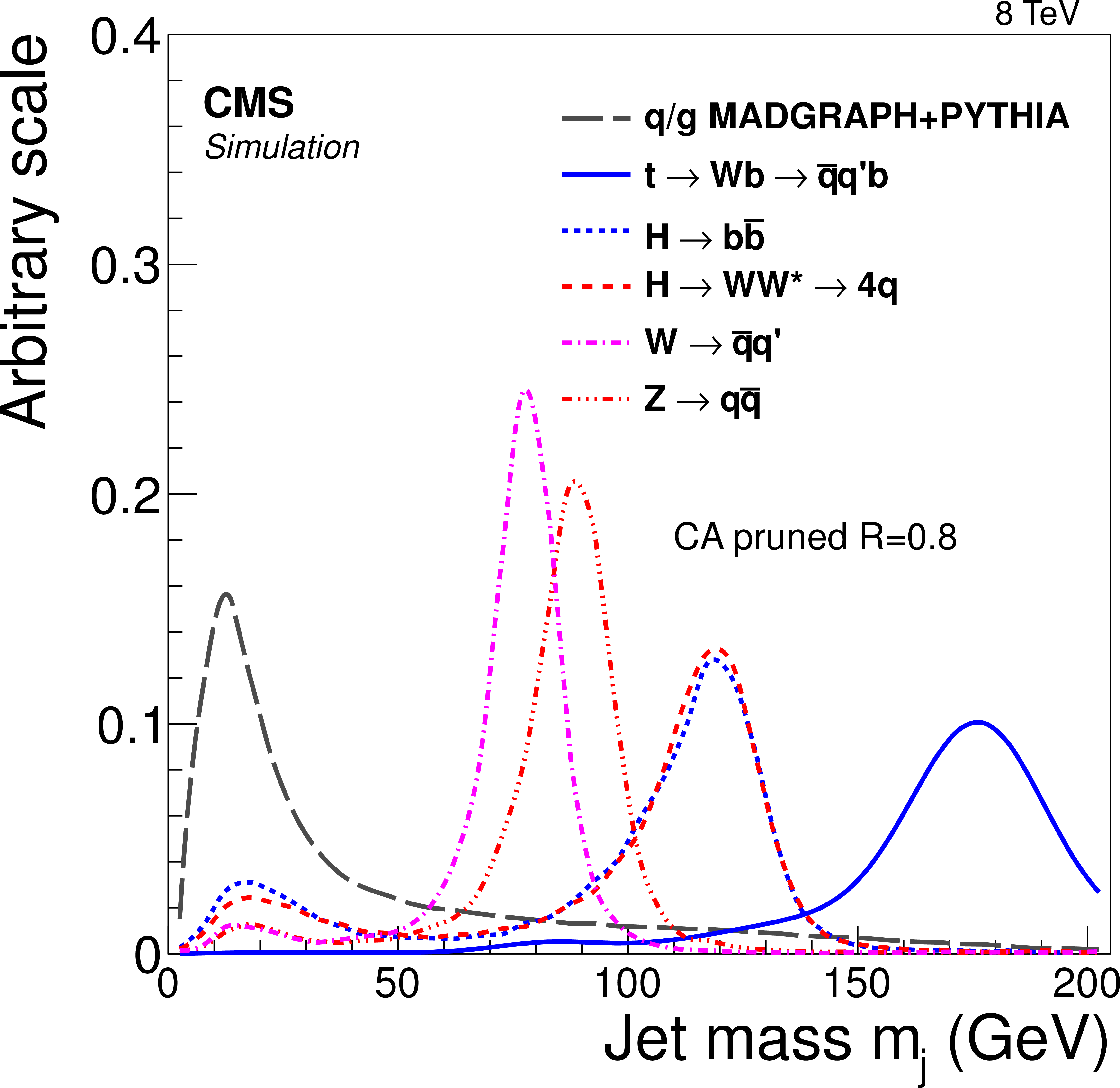
Figure 2:
Distribution of pruned jet mass in simulation of signal and background processes. All simulated distributions are normalized to 1. The W/Z, H, and top-quark jets are required to match respective generator level particles in the event. The W/Z and H jets are from 1.5 TeV $ {\mathrm {W}^\prime } \to {\mathrm {W}} {\mathrm {H}} $ and $ {\mathrm {Z}^\prime }\to {\mathrm {Z}} {\mathrm {H}} $ signal samples. |

png pdf |
Figure 3-a:
Distributions of $\tau _{42}$ in data and in simulations of signal (2 TeV) and background events, without applying the pruned jet mass requirement (a) and with the pruned jet mass requirement applied (b). Matched top-quark, W/Z, and $ {\mathrm {H}}_{ {\mathrm {W}} {\mathrm {W}}}$ jets are required to be consistent with their generator level particles, respectively. All simulated distributions are scaled to the number of events in data, except that matched top-quark background is scaled to the fraction of unmatched $ {\mathrm {t}\overline {\mathrm {t}}} $ events times the number of data events. |

png pdf |
Figure 3-b:
Distributions of $\tau _{42}$ in data and in simulations of signal (2 TeV) and background events, without applying the pruned jet mass requirement (a) and with the pruned jet mass requirement applied (b). Matched top-quark, W/Z, and $ {\mathrm {H}}_{ {\mathrm {W}} {\mathrm {W}}}$ jets are required to be consistent with their generator level particles, respectively. All simulated distributions are scaled to the number of events in data, except that matched top-quark background is scaled to the fraction of unmatched $ {\mathrm {t}\overline {\mathrm {t}}} $ events times the number of data events. |

png pdf |
Figure 4:
Comparison of $\tau _{42}$ distributions for signal events failing the $ { {\mathrm {H}} \to { {\mathrm {b}} {\overline {\mathrm {b}}}} }$ requirement. These events are from the $ { {\mathrm {H}} \to {\mathrm {W}} {\mathrm {W}}^*\to 4{ {\mathrm {q}} }}$, $ { {\mathrm {H}} \to { {\mathrm {b}} {\overline {\mathrm {b}}}} }$, $ {\mathrm {H}} \to {\mathrm {g}} {\mathrm {g}} $, $ {\mathrm {H}} \to {\mathrm {c}} {\overline {\mathrm {c}}} $, and $ {\mathrm {H}} \to \tau \tau $ channels. The H jets are from a 1.5 TeV resonance decaying to VH. All curves are normalized to the product of the corresponding branching fraction and acceptance. |

png pdf |
Figure 5-a:
Tagged fractions in $ { { {\mathrm {H}} \to { {\mathrm {b}} {\overline {\mathrm {b}}}} } }$, $ { {\mathrm {W}} / {\mathrm {Z}} \to {\overline {\mathrm {q}}} {\mathrm {q}}'}$ signal channels and data as a function of dijet invariant mass, for categories of $ {\mathrm {V^{HP} H_{bb}}} $ (a) and $ {\mathrm {V^{LP} H_{bb} }} $ (b). Horizontal bars through the data points indicate the bin width. |

png pdf |
Figure 5-b:
Tagged fractions in $ { { {\mathrm {H}} \to { {\mathrm {b}} {\overline {\mathrm {b}}}} } }$, $ { {\mathrm {W}} / {\mathrm {Z}} \to {\overline {\mathrm {q}}} {\mathrm {q}}'}$ signal channels and data as a function of dijet invariant mass, for categories of $ {\mathrm {V^{HP} H_{bb}}} $ (a) and $ {\mathrm {V^{LP} H_{bb} }} $ (b). Horizontal bars through the data points indicate the bin width. |

png pdf |
Figure 6-a:
Tagged fractions in $ { { {\mathrm {H}} \to {\mathrm {W}} {\mathrm {W}}^*\to 4{ {\mathrm {q}} }} }$, $ { {\mathrm {W}}/ {\mathrm {Z}}\to {\overline {\mathrm {q}}} {\mathrm {q}}'}$ signal channels and data as a function of dijet invariant mass, for categories of $ {\mathrm {V^{HP} H_{WW}^{HP}}}$ (a), $ {\mathrm {V^{HP} H_{WW}^{LP}}}$ (b) and $ {\mathrm {V^{LP} H_{WW}^{HP}}}$ (c). Horizontal bars through the data points indicate the bin width. |

png pdf |
Figure 6-b:
Tagged fractions in $ { { {\mathrm {H}} \to {\mathrm {W}} {\mathrm {W}}^*\to 4{ {\mathrm {q}} }} }$, $ { {\mathrm {W}}/ {\mathrm {Z}}\to {\overline {\mathrm {q}}} {\mathrm {q}}'}$ signal channels and data as a function of dijet invariant mass, for categories of $ {\mathrm {V^{HP} H_{WW}^{HP}}}$ (a), $ {\mathrm {V^{HP} H_{WW}^{LP}}}$ (b) and $ {\mathrm {V^{LP} H_{WW}^{HP}}}$ (c). Horizontal bars through the data points indicate the bin width. |

png pdf |
Figure 6-c:
Tagged fractions in $ { { {\mathrm {H}} \to {\mathrm {W}} {\mathrm {W}}^*\to 4{ {\mathrm {q}} }} }$, $ { {\mathrm {W}}/ {\mathrm {Z}}\to {\overline {\mathrm {q}}} {\mathrm {q}}'}$ signal channels and data as a function of dijet invariant mass, for categories of $ {\mathrm {V^{HP} H_{WW}^{HP}}}$ (a), $ {\mathrm {V^{HP} H_{WW}^{LP}}}$ (b) and $ {\mathrm {V^{LP} H_{WW}^{HP}}}$ (c). Horizontal bars through the data points indicate the bin width. |
png pdf |
Figure 7-a:
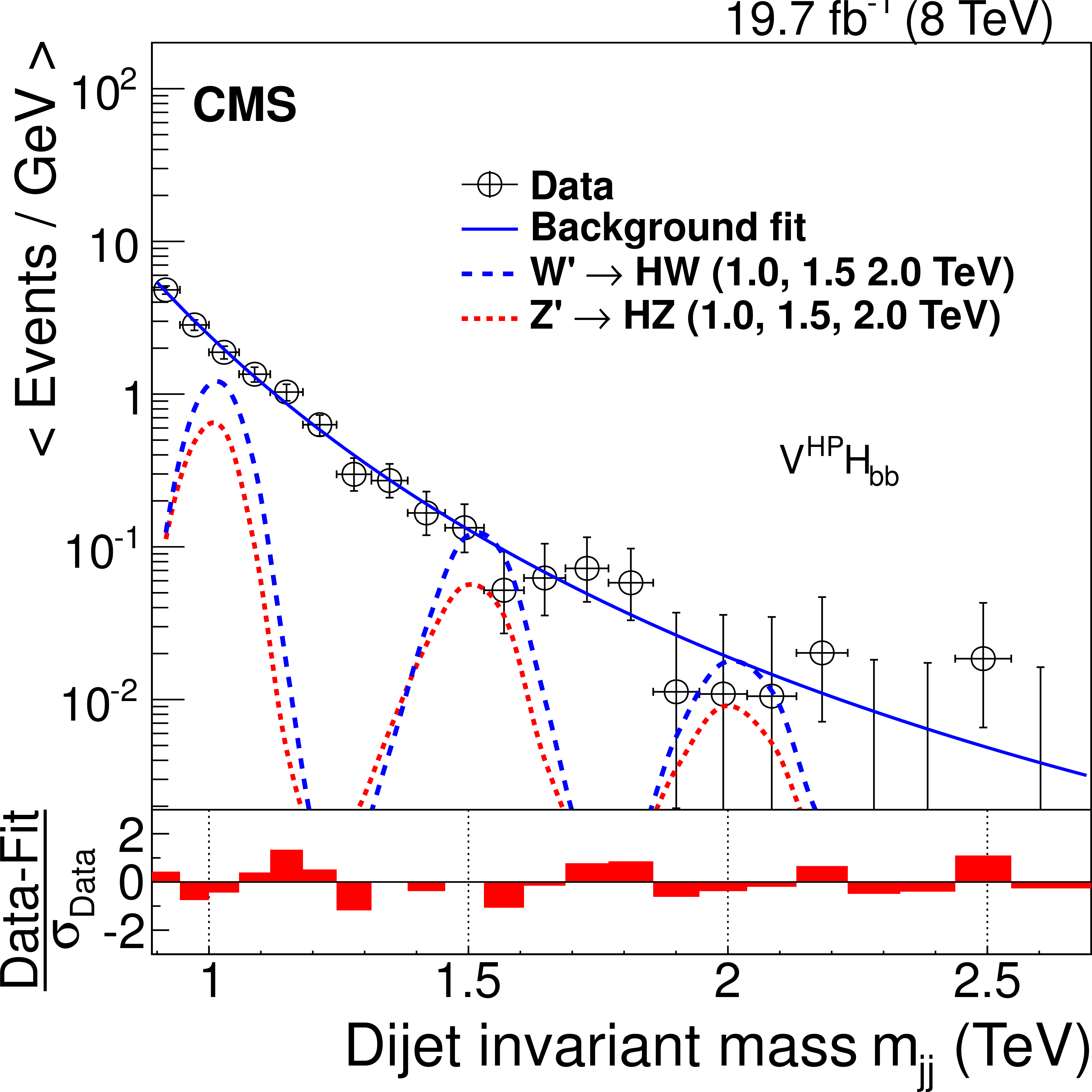
Distributions in $m_\mathrm {jj}$ are shown for $ {\mathrm {V^{HP} H_{bb}}}$ category (a), $ {\mathrm {V^{LP} H_{bb} }}$ category (b). The solid curves represent the results of fitting Eq.(2) to the data. The distributions for $ { { {\mathrm {H}} \to { {\mathrm {b}} {\overline {\mathrm {b}}}} } }$, $ { {\mathrm {W}}/ {\mathrm {Z}}\to {\overline {\mathrm {q}}} {\mathrm {q}}'}$ contributions, scaled to their corresponding cross sections, are given by the dashed curves. The vertical axis displays the number of events per bin, divided by the bin width. Horizontal bars through the data points indicate the bin width. The corresponding pull distributions $\frac {\text {Data}-\text {Fit}}{\sigma _{\text {Data}}}$, where $\sigma _{\text {Data}}$ represents the statistical uncertainty in the data in a bin in $m_\mathrm {jj}$, are shown below each $m_\mathrm {jj}$ plot. |
png pdf |
Figure 7-b:
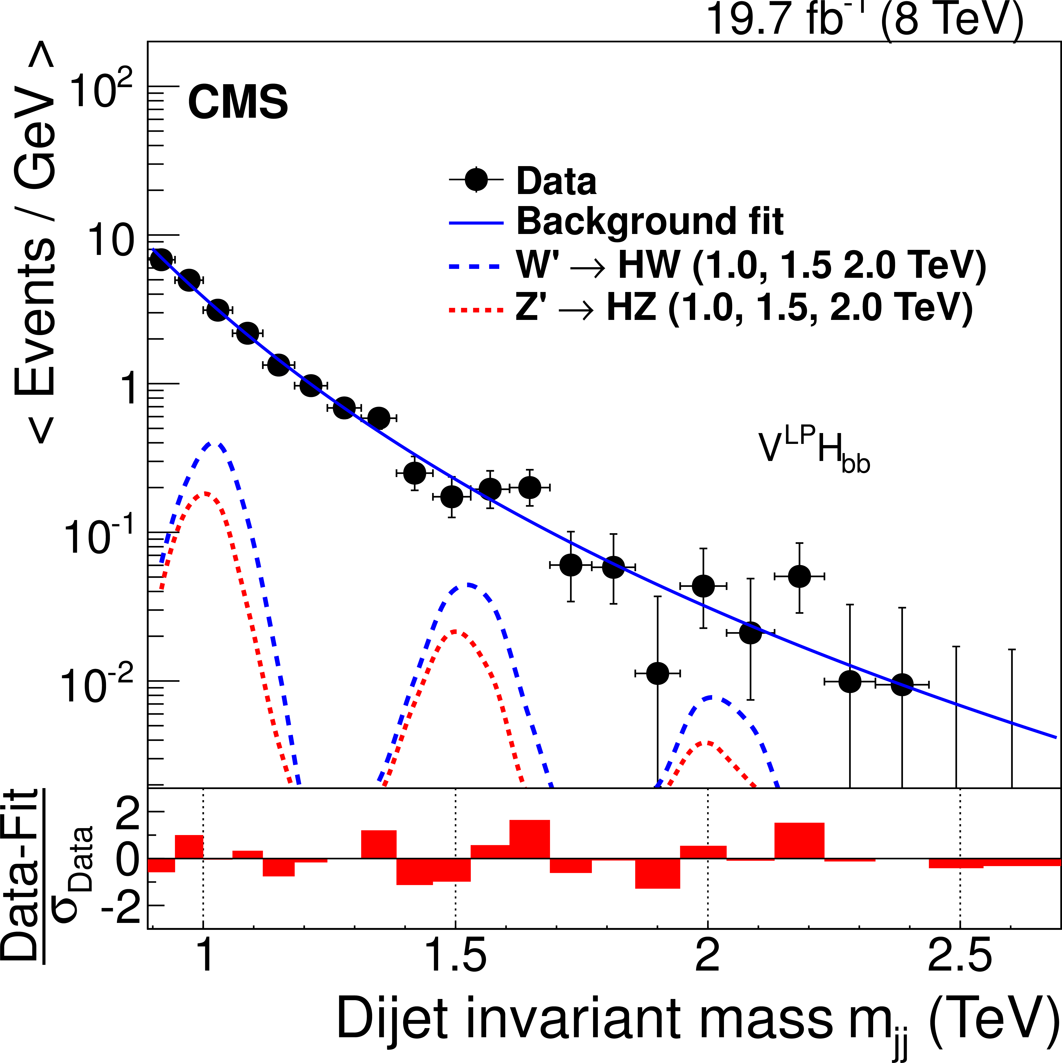
Distributions in $m_\mathrm {jj}$ are shown for $ {\mathrm {V^{HP} H_{bb}}}$ category (a), $ {\mathrm {V^{LP} H_{bb} }}$ category (b). The solid curves represent the results of fitting Eq.(2) to the data. The distributions for $ { { {\mathrm {H}} \to { {\mathrm {b}} {\overline {\mathrm {b}}}} } }$, $ { {\mathrm {W}}/ {\mathrm {Z}}\to {\overline {\mathrm {q}}} {\mathrm {q}}'}$ contributions, scaled to their corresponding cross sections, are given by the dashed curves. The vertical axis displays the number of events per bin, divided by the bin width. Horizontal bars through the data points indicate the bin width. The corresponding pull distributions $\frac {\text {Data}-\text {Fit}}{\sigma _{\text {Data}}}$, where $\sigma _{\text {Data}}$ represents the statistical uncertainty in the data in a bin in $m_\mathrm {jj}$, are shown below each $m_\mathrm {jj}$ plot. |

png pdf |
Figure 8-a:
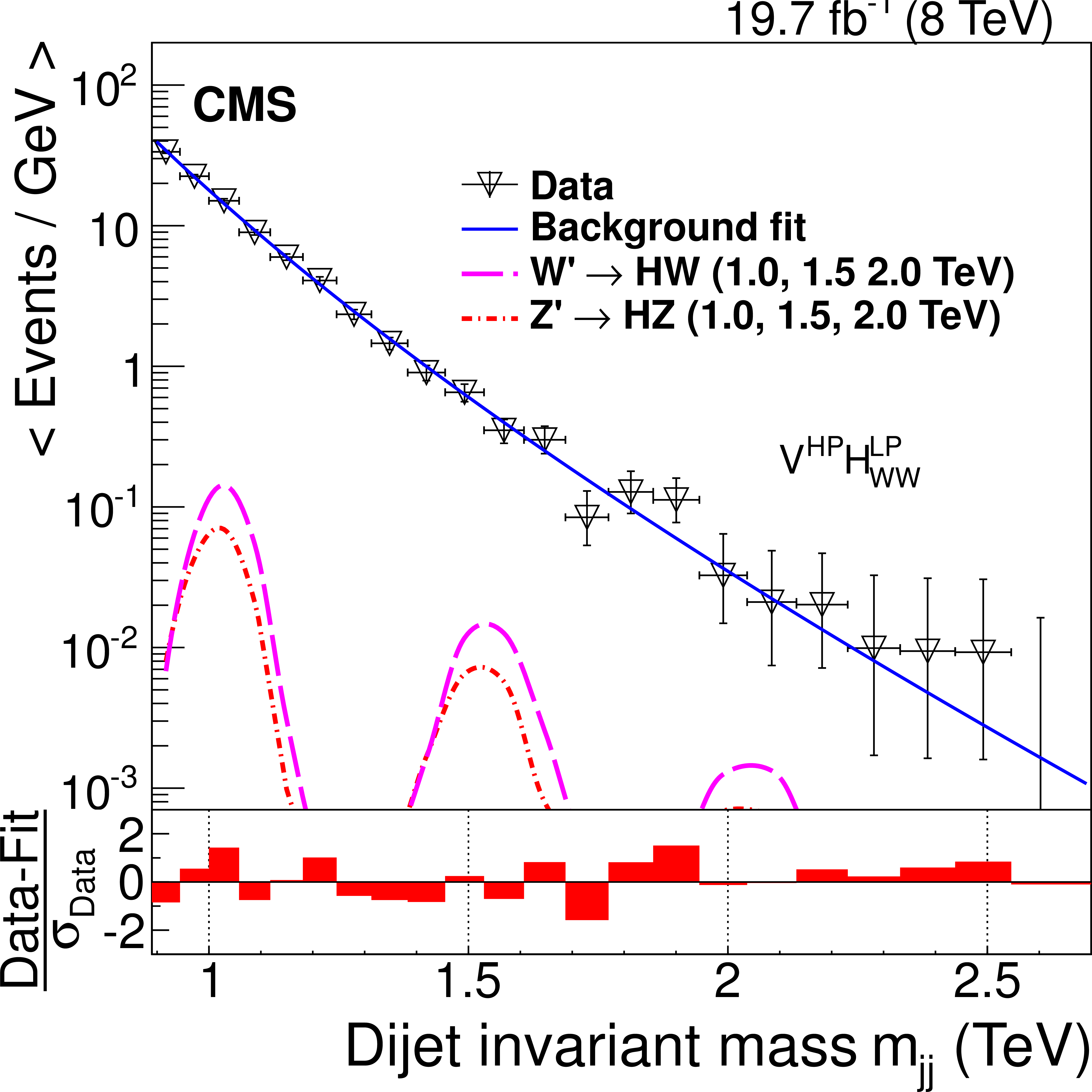
Distributions in $m_\mathrm {jj}$ are shown for $ {\mathrm {V^{HP} H_{WW}^{HP}}}$ (a), $ {\mathrm {V^{HP} H_{WW}^{LP}}} $ (b), and $ {\mathrm {V^{LP} H_{WW}^{HP}}}$ (c). The solid curves represent the results of fitting Eq.(2) to the data. The distributions for $ { { {\mathrm {H}} \to {\mathrm {W}} {\mathrm {W}}^*\to 4{ {\mathrm {q}} }}}$, $ { {\mathrm {W}}/ {\mathrm {Z}}\to {\overline {\mathrm {q}}} {\mathrm {q}}'}$ contributions, scaled to their corresponding cross sections, are given by the dashed and dash-dotted curves. The vertical axis displays the number of events per bin, divided by the bin width. Horizontal bars through the data points indicate the bin width. The corresponding pull distributions $\frac {\text {Data}-\text {Fit}}{\sigma _{\text {Data}}}$, where $\sigma _{\text {Data}}$ represents the statistical uncertainty in the data in a bin in $m_\mathrm {jj}$, are shown below each $m_\mathrm {jj}$ plot. |
png pdf |
Figure 8-b:
Distributions in $m_\mathrm {jj}$ are shown for $ {\mathrm {V^{HP} H_{WW}^{HP}}}$ (a), $ {\mathrm {V^{HP} H_{WW}^{LP}}} $ (b), and $ {\mathrm {V^{LP} H_{WW}^{HP}}}$ (c). The solid curves represent the results of fitting Eq.(2) to the data. The distributions for $ { { {\mathrm {H}} \to {\mathrm {W}} {\mathrm {W}}^*\to 4{ {\mathrm {q}} }}}$, $ { {\mathrm {W}}/ {\mathrm {Z}}\to {\overline {\mathrm {q}}} {\mathrm {q}}'}$ contributions, scaled to their corresponding cross sections, are given by the dashed and dash-dotted curves. The vertical axis displays the number of events per bin, divided by the bin width. Horizontal bars through the data points indicate the bin width. The corresponding pull distributions $\frac {\text {Data}-\text {Fit}}{\sigma _{\text {Data}}}$, where $\sigma _{\text {Data}}$ represents the statistical uncertainty in the data in a bin in $m_\mathrm {jj}$, are shown below each $m_\mathrm {jj}$ plot. |

png pdf |
Figure 8-c:
Distributions in $m_\mathrm {jj}$ are shown for $ {\mathrm {V^{HP} H_{WW}^{HP}}}$ (a), $ {\mathrm {V^{HP} H_{WW}^{LP}}} $ (b), and $ {\mathrm {V^{LP} H_{WW}^{HP}}}$ (c). The solid curves represent the results of fitting Eq.(2) to the data. The distributions for $ { { {\mathrm {H}} \to {\mathrm {W}} {\mathrm {W}}^*\to 4{ {\mathrm {q}} }}}$, $ { {\mathrm {W}}/ {\mathrm {Z}}\to {\overline {\mathrm {q}}} {\mathrm {q}}'}$ contributions, scaled to their corresponding cross sections, are given by the dashed and dash-dotted curves. The vertical axis displays the number of events per bin, divided by the bin width. Horizontal bars through the data points indicate the bin width. The corresponding pull distributions $\frac {\text {Data}-\text {Fit}}{\sigma _{\text {Data}}}$, where $\sigma _{\text {Data}}$ represents the statistical uncertainty in the data in a bin in $m_\mathrm {jj}$, are shown below each $m_\mathrm {jj}$ plot. |

png pdf |
Figure 9-a:
Expected and observed upper limits on the production cross sections for $ {\mathrm {Z}^\prime }\to {\mathrm {H}} {\mathrm {Z}} $ (a) and $ {\mathrm {W}^\prime } \to {\mathrm {H}} {\mathrm {W}}$ (b), including all five decay categories. Branching fractions of H and V decays have been taken into account. The theoretical predictions of the HVT model scenario B are also shown. |
png pdf |
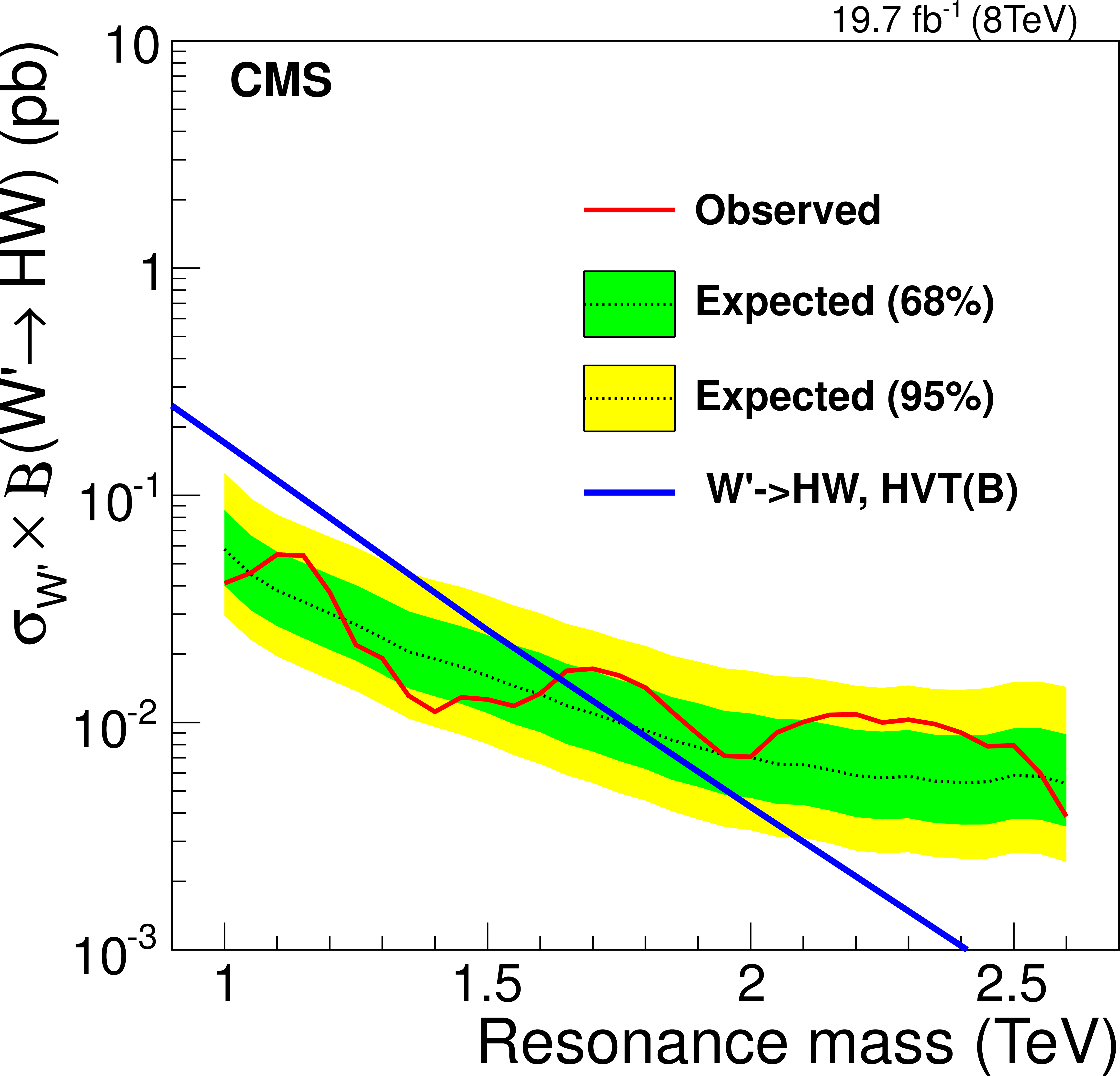
Figure 9-b:
Expected and observed upper limits on the production cross sections for $ {\mathrm {Z}^\prime }\to {\mathrm {H}} {\mathrm {Z}} $ (a) and $ {\mathrm {W}^\prime } \to {\mathrm {H}} {\mathrm {W}}$ (b), including all five decay categories. Branching fractions of H and V decays have been taken into account. The theoretical predictions of the HVT model scenario B are also shown. |

png pdf |
Figure 10:
Expected and observed upper limits on the production cross section for ${\mathrm{ V'\to VH}}$, obtained by combining $ {\mathrm {W}^\prime } $ and $ {\mathrm {Z}^\prime }$ channels together. Branching fractions of H and V decays have been taken into account. The theoretical prediction of the HVT model scenario B is also shown. |
| Tables | |

png pdf |
Table 1:
Summary of event categories and their nomenclature used in the paper. The jet mass cut is $70 < m_j <100 $ GeV/$c^2$ for the V tag and $110 < m_j < 135$ GeV/$c^2$ for the H tag. |

png pdf |
Table 2:
Summary of the values $P$ for a Z? signal at 1.5 TeV resonance mass and the corresponding background yield in all five categories. |

png pdf |
Table 3:
Systematic uncertainties common to all categories. |

png pdf |
Table 4:
Systematic uncertainties(%) for $\mathrm{ X \to VH }$ signals, in which $\mathrm{ H \to b \overline{b} }$ and $\mathrm{ H \to WW^* \to 4q }$. Numbers in parentheses represent the uncertainty for the corresponding LP category. If LP has the same uncertainty as HP, only the HP uncertainty is presented here. |

png pdf |
Table 5:
Summary of observed lower limits on resonance masses at 95% CL and their expected values, assuming a null hypothesis. The analysis is sensitive to resonances heavier than 1 TeV. |
| Summary |
|
A search for a massive resonance decaying into a standard model-like Higgs boson and a W or Z boson is presented. A data sample corresponding to an integrated luminosity of 19.7 fb$^{-1}$ collected in proton-proton collisions at $\sqrt{s} =$ 8 TeV with the CMS detector has been used to measure the W/Z and Higgs boson-tagged dijet mass spectra using the two highest $p_{\mathrm{T}}$ jets within the pseudorapidity range $ |\eta| < 2.5$ and with pseudorapidity separation $ | \Delta \eta | < 1.3$. The QCD background is suppressed using jet substructure tagging techniques, which identify boosted bosons decaying into hadrons. In particular, the mass of pruned jets and the N-subjettiness ratios $\tau_{21}$ and $\tau_{42}$, as well as b tagging applied to the subjets of the Higgs boson jet, are used to discriminate against the otherwise overwhelming QCD background. The remaining QCD background is estimated from a fit to the dijet mass distributions using a smooth function. We have searched for the signal as a peak on top of the smoothly falling QCD background. No significant signal is observed. In the HVT model B, a Z′ is excluded in resonance mass intervals [1.0, 1.1] and [1.3, 1.5] TeV, while a W′ is excluded in the interval [1.0, 1.6] TeV. A mass degenerate W′ plus Z′ particle is excluded in the interval [1.0, 1.7] TeV. This is the first search for heavy resonances decaying into a Higgs boson and a vector boson (W/Z) resulting in a hadronic final state, as well as the first application of jet substructure techniques to identify $\mathrm{ H \to WW^∗ \to 4q}$ decays of the Higgs boson at high Lorentz boost. |
|
|
Compact Muon Solenoid LHC, CERN |
|

|

|

|

|

|