

Compact Muon Solenoid
LHC, CERN
| CMS-HIG-11-019 ; CERN-PH-EP-2012-123 | ||
| Search for a light charged Higgs boson in top quark decays in pp collisions at $\sqrt{s}$ = 7 TeV | ||
| CMS Collaboration | ||
| 25 May 2012 | ||
| J. High Energy Phys. 07 (2012) 143 | ||
| Abstract: Results are presented on a search for a light charged Higgs boson that can be produced in the decay of the top quark to charged H and b quark and which, in turn, decays into tau and tau neutrino. The analysed data correspond to an integrated luminosity of about 2 inverse femtobarns recorded in proton-proton collisions at sqrt(s) = 7 TeV by the CMS experiment at the LHC. The search is sensitive to the decays of the top quark pairs t anti-t to charged Higgs W b anti-b and t anti-t to charged Higgs b anti-b. Various final states have been studied separately, all requiring presence of a tau lepton from charged Higgs decays, missing transverse energy, and multiple jets. Upper limits on the branching fraction B(t to charged Higgs b) in the range of 2-3% are established for charged Higgs boson masses between 80 and 160 GeV, under the assumption that B(charged Higgs to tau anti-tau) = 1. | ||
| Links: e-print arXiv:1205.5736 [hep-ex] (PDF) ; CDS record ; inSPIRE record ; Public twiki page ; CADI line (restricted) ; | ||
| Figures | |
png pdf |
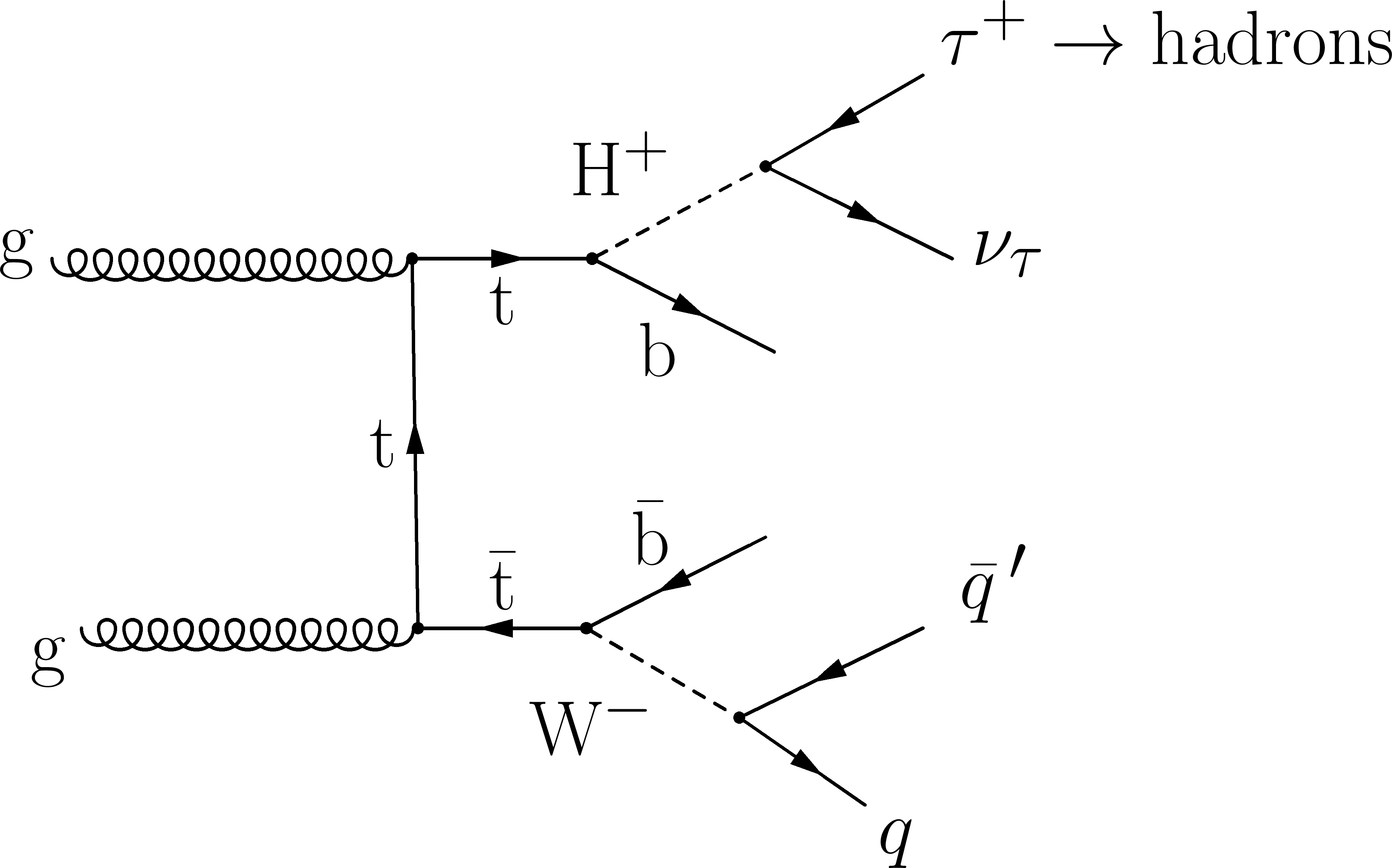
Figure 1-a:
Representative diagrams for the $ {\tau }_\mathrm {h}$+jets (a), $ {\mathrm {e}}( {{\mu }}) {\tau }_\mathrm {h}$ (b), and $ {\mathrm {e}} {{\mu }}$ (c) final states. |
png pdf |
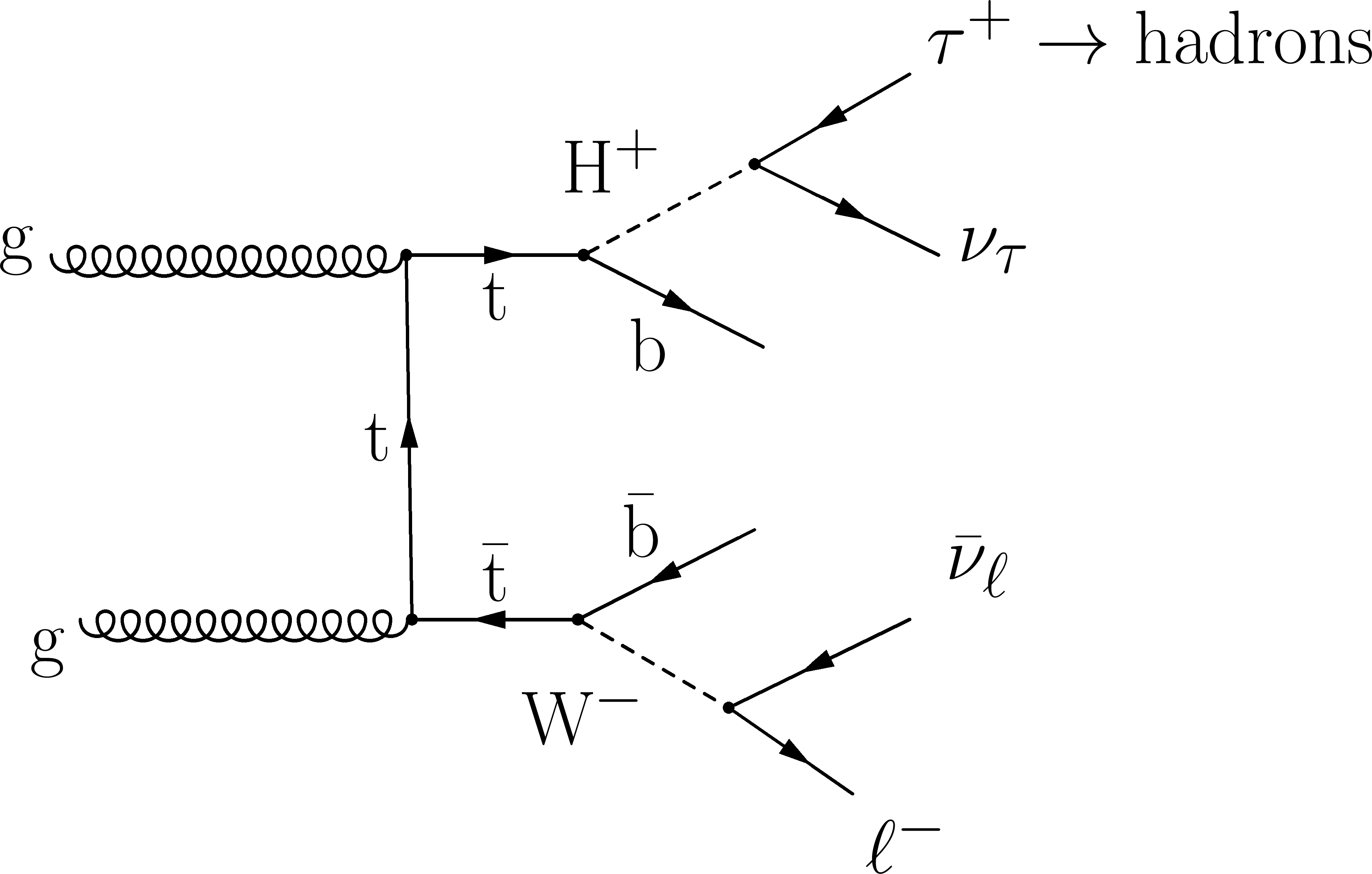
Figure 1-b:
Representative diagrams for the $ {\tau }_\mathrm {h}$+jets (a), $ {\mathrm {e}}( {{\mu }}) {\tau }_\mathrm {h}$ (b), and $ {\mathrm {e}} {{\mu }}$ (c) final states. |
png pdf |
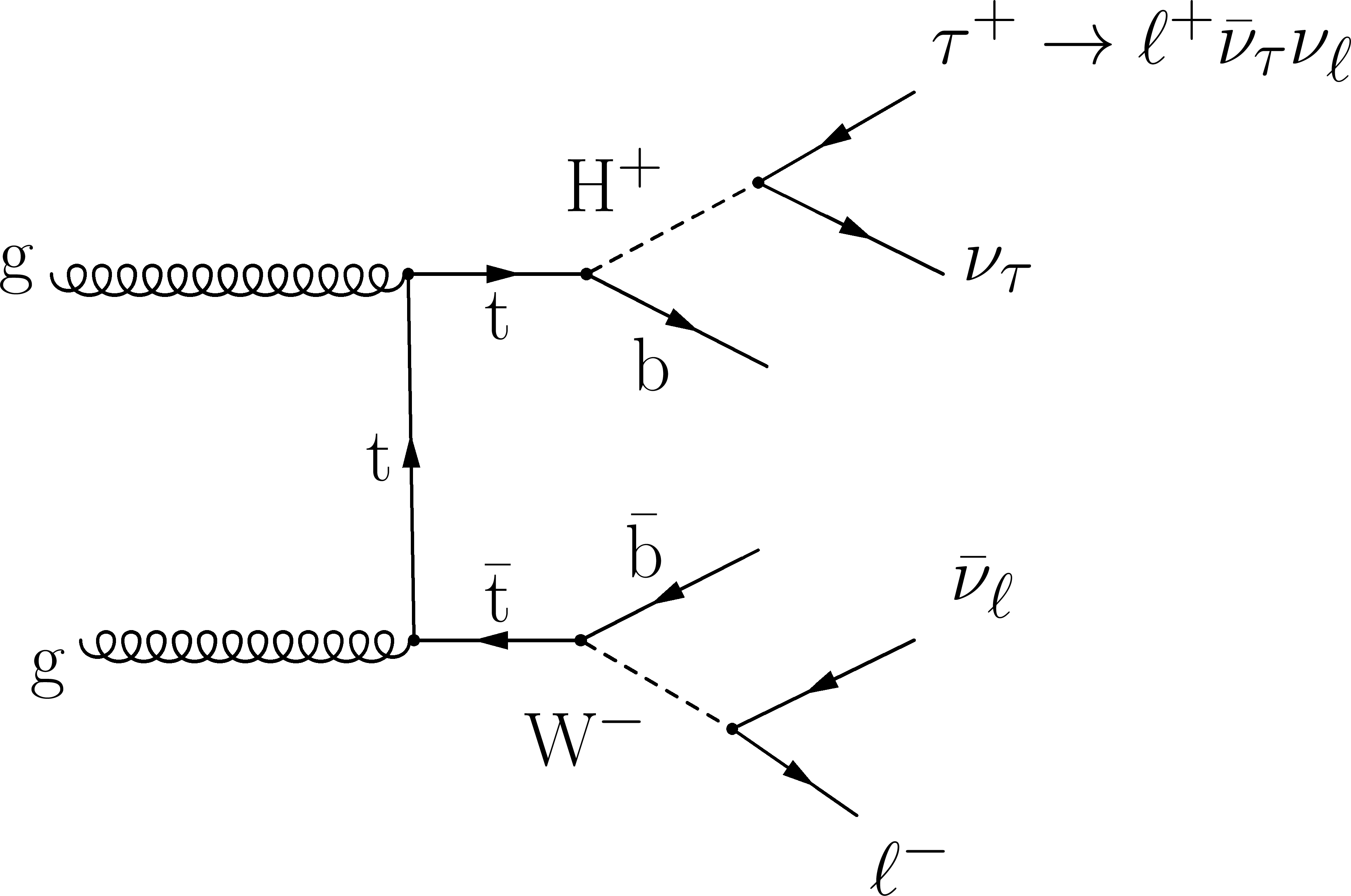
Figure 1-c:
Representative diagrams for the $ {\tau }_\mathrm {h}$+jets (a), $ {\mathrm {e}}( {{\mu }}) {\tau }_\mathrm {h}$ (b), and $ {\mathrm {e}} {{\mu }}$ (c) final states. |

png |
Figure 1:
|
png pdf |
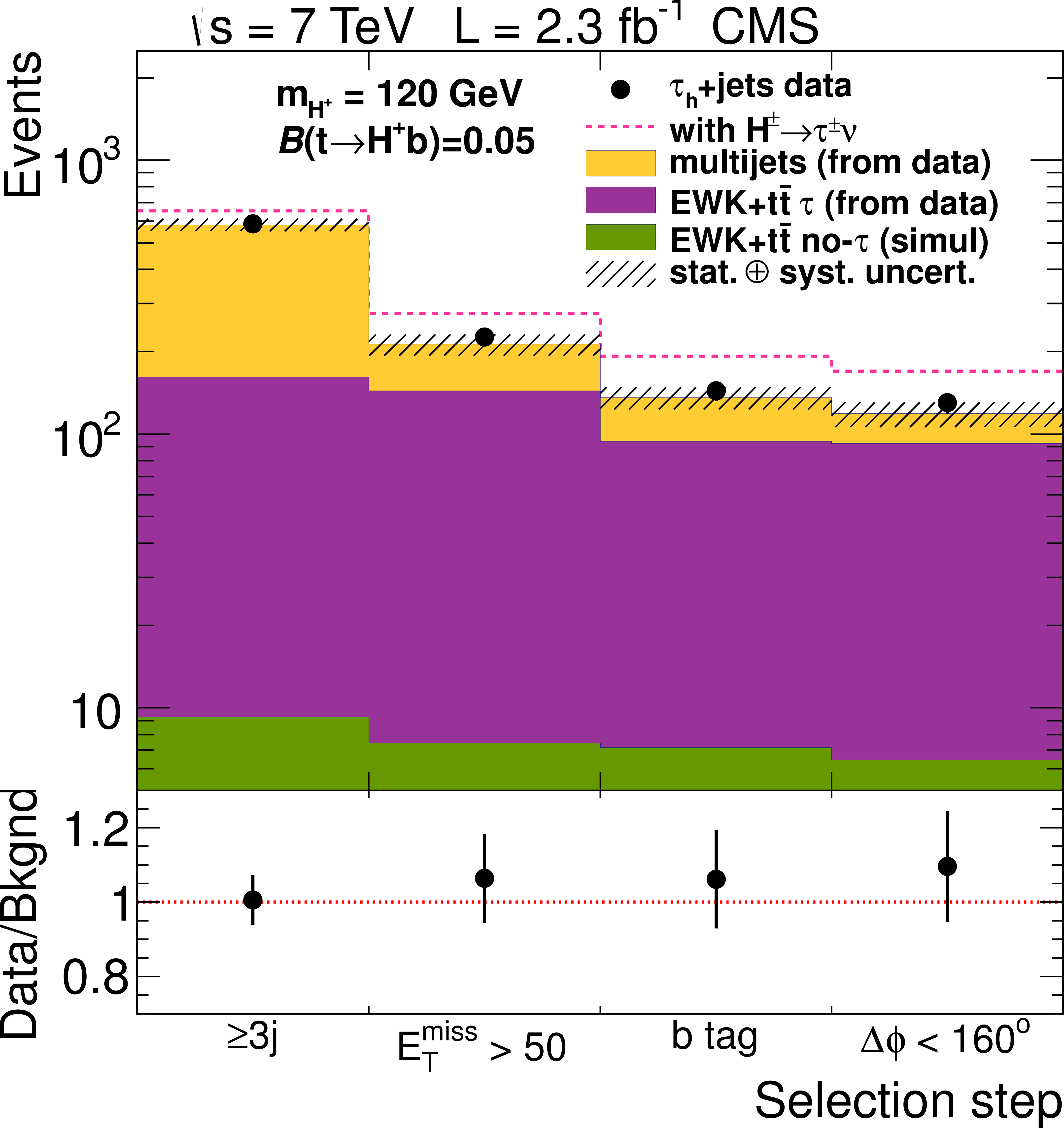
Figure 2:
The event yield after each selection step for the $ {\tau }_\mathrm {h}$+jets analysis. The expected event yield in the presence of the $ {\mathrm {t}}\rightarrow {\mathrm {H}} ^{+} {\mathrm {b}}$, $ {\mathrm {H}} ^{+}\rightarrow {\tau }^{+} {\nu _{\tau }}$ decays is shown as the dashed line for $m_{ {\mathrm {H}} ^{+}} =$ 120 GeV and under that assumption that $\mathcal {B}( {\mathrm {t}}\rightarrow {\mathrm {H}} ^{+} {\mathrm {b}}) =$ 0.05. The multijet and the ``EWK+$ {\mathrm {t}\overline {\mathrm {t}}} $ $ {\tau }$" backgrounds are measured from the data. The ``EWK+$ {\mathrm {t}\overline {\mathrm {t}}} $ no-$ {\tau }$" background is shown as estimated from simulation. The bottom panel shows the ratio of data over background along with the total uncertainties. Statistical and systematic uncertainties are added in quadrature. |
png pdf |
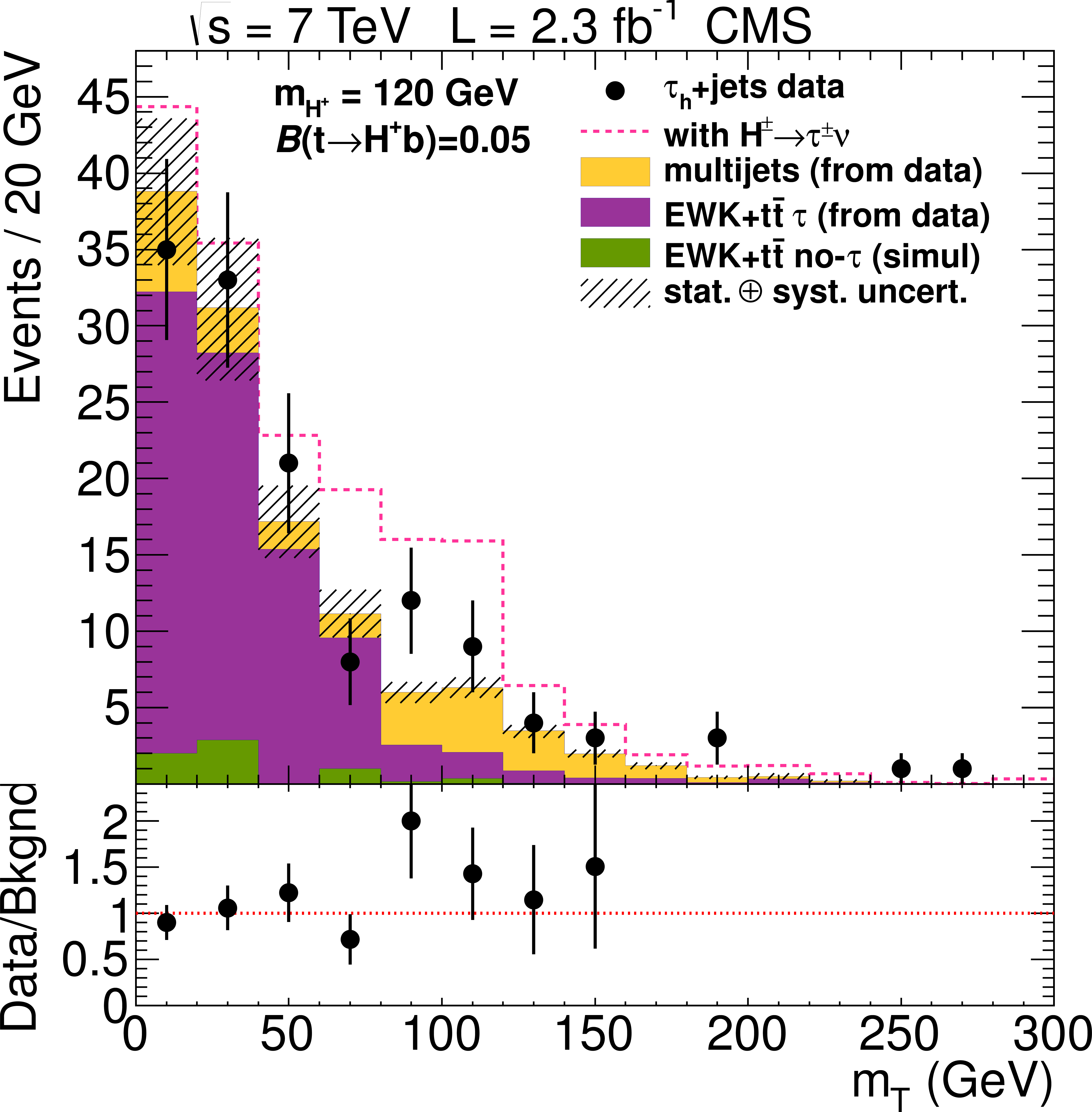
Figure 3:
The transverse mass of $ {\tau }_\mathrm {h}$ and $ {E_{\mathrm {T}}^{\text {miss}}} $ after full event selection for the $ {\tau }_\mathrm {h}$+jets analysis. The expected event yield in the presence of the $ {\mathrm {t}}\rightarrow {\mathrm {H}} ^{+} {\mathrm {b}}$, $ {\mathrm {H}} ^{+}\rightarrow {\tau }^{+} {\nu }$ decays is shown as the dashed line for $m_{ {\mathrm {H}} ^{+}} =$ 120 GeV and under the assumption that $\mathcal {B}( {\mathrm {t}}\rightarrow {\mathrm {H}} ^{+} {\mathrm {b}}) =$ 0.05. The bottom panel shows the ratio of data over background along with the total uncertainties. The ratio is not shown for $ {m_\mathrm {T}}> $160 GeV, where the expected total number of the background events is 2.5 $\pm$ 0.3 while 5 events are observed. Statistical and systematic uncertainties are always added in quadrature. |
png pdf |
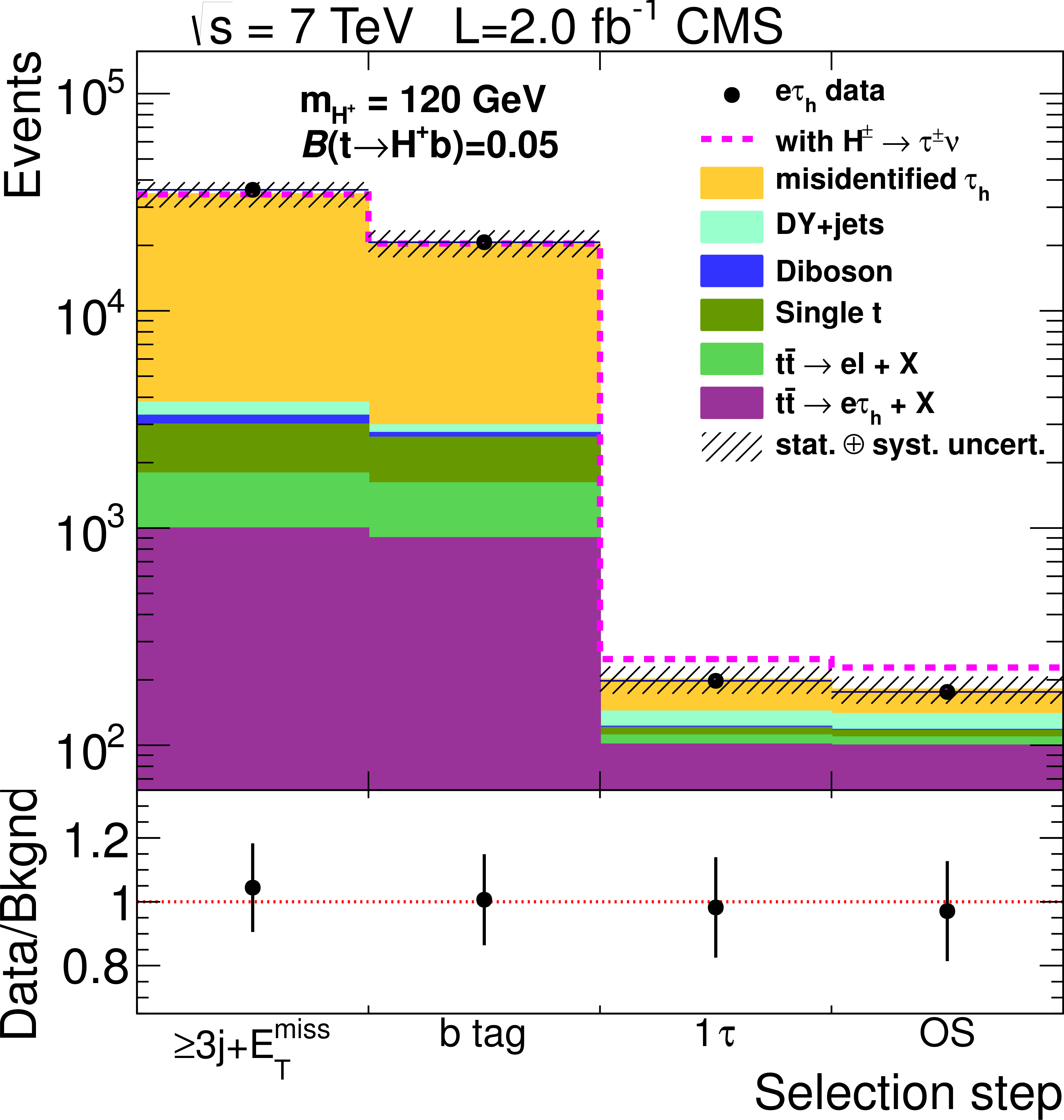
Figure 4-a:
The event yields after each selection step for the $ {\mathrm {e}} {\tau }_\mathrm {h}$ (a) and $ {{\mu }} {\tau }_\mathrm {h}$ (b) analyses. The backgrounds are estimated from simulation and normalized to the standard model prediction. The expected event yield in the presence of the $ {\mathrm {t}}\rightarrow {\mathrm {H}} ^{+} {\mathrm {b}}$, $ {\mathrm {H}} ^{+}$$\rightarrow {\tau }^{+} {\nu _{\tau }}$ decays is shown as a dashed line for $m_{ {\mathrm {H}} ^{+}} =$ 120 GeV and under the assumption that $\mathcal {B}( {\mathrm {t}}\rightarrow {\mathrm {H}} ^{+} {\mathrm {b}}) =$ 0.05. The bottom panel shows the ratios of data over background with the total uncertainties. OS indicates the requirement to have opposite electric charges for a $ {\tau }_\mathrm {h}$ and a $ {\mathrm {e}}$ or $ {{\mu }}$. Statistical and systematic uncertainties are added in quadrature. |
png pdf |
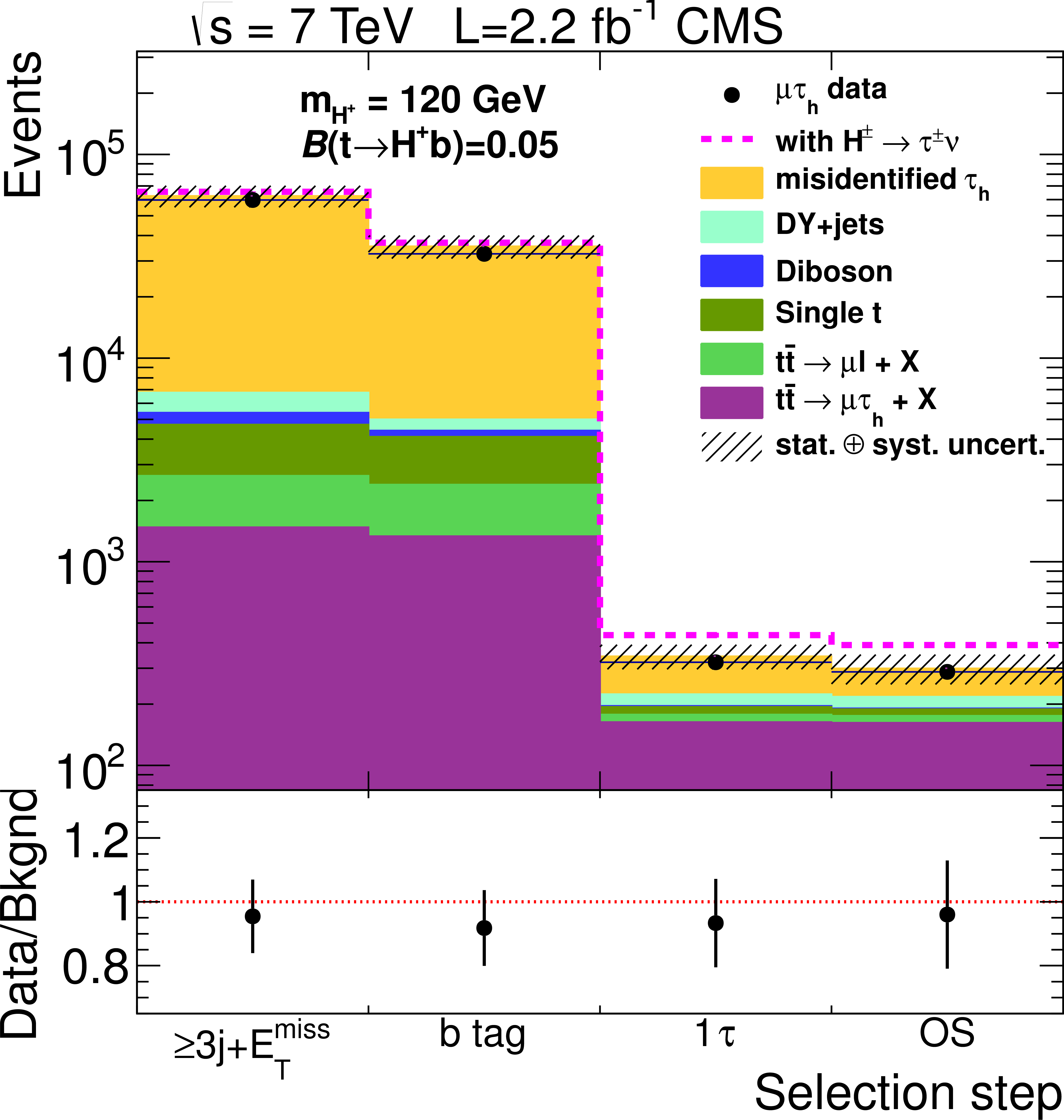
Figure 4-b:
The event yields after each selection step for the $ {\mathrm {e}} {\tau }_\mathrm {h}$ (a) and $ {{\mu }} {\tau }_\mathrm {h}$ (b) analyses. The backgrounds are estimated from simulation and normalized to the standard model prediction. The expected event yield in the presence of the $ {\mathrm {t}}\rightarrow {\mathrm {H}} ^{+} {\mathrm {b}}$, $ {\mathrm {H}} ^{+}$$\rightarrow {\tau }^{+} {\nu _{\tau }}$ decays is shown as a dashed line for $m_{ {\mathrm {H}} ^{+}} =$ 120 GeV and under the assumption that $\mathcal {B}( {\mathrm {t}}\rightarrow {\mathrm {H}} ^{+} {\mathrm {b}}) =$ 0.05. The bottom panel shows the ratios of data over background with the total uncertainties. OS indicates the requirement to have opposite electric charges for a $ {\tau }_\mathrm {h}$ and a $ {\mathrm {e}}$ or $ {{\mu }}$. Statistical and systematic uncertainties are added in quadrature. |

png |
Figure 4:
|

png pdf |
Figure 5:
The event yield after each selection step for the $ {\mathrm {e}} {{\mu }}$ analysis. The backgrounds are from simulation and normalized to the standard model prediction. The expected event yield in the presence of the $ {\mathrm {t}}\rightarrow {\mathrm {H}} ^{+} {\mathrm {b}}$, $ {\mathrm {H}} ^{+}\rightarrow {\tau }^{+} {\nu _{\tau }}$ decays is shown as a dashed line for $m_{ {\mathrm {H}} ^{+}}=$ 120 GeV under the assumption that $\mathcal {B}( {\mathrm {t}}\rightarrow {\mathrm {H}} ^{+} {\mathrm {b}}) =$ 0.05. The bottom panel shows the ratios of data over background with the total uncertainties. The requirement for the $ {\mathrm {e}}$ and $ {{\mu }}$ to have opposite electric charges is labelled as OS. Statistical and systematic uncertainties are added in quadrature. |
png pdf |
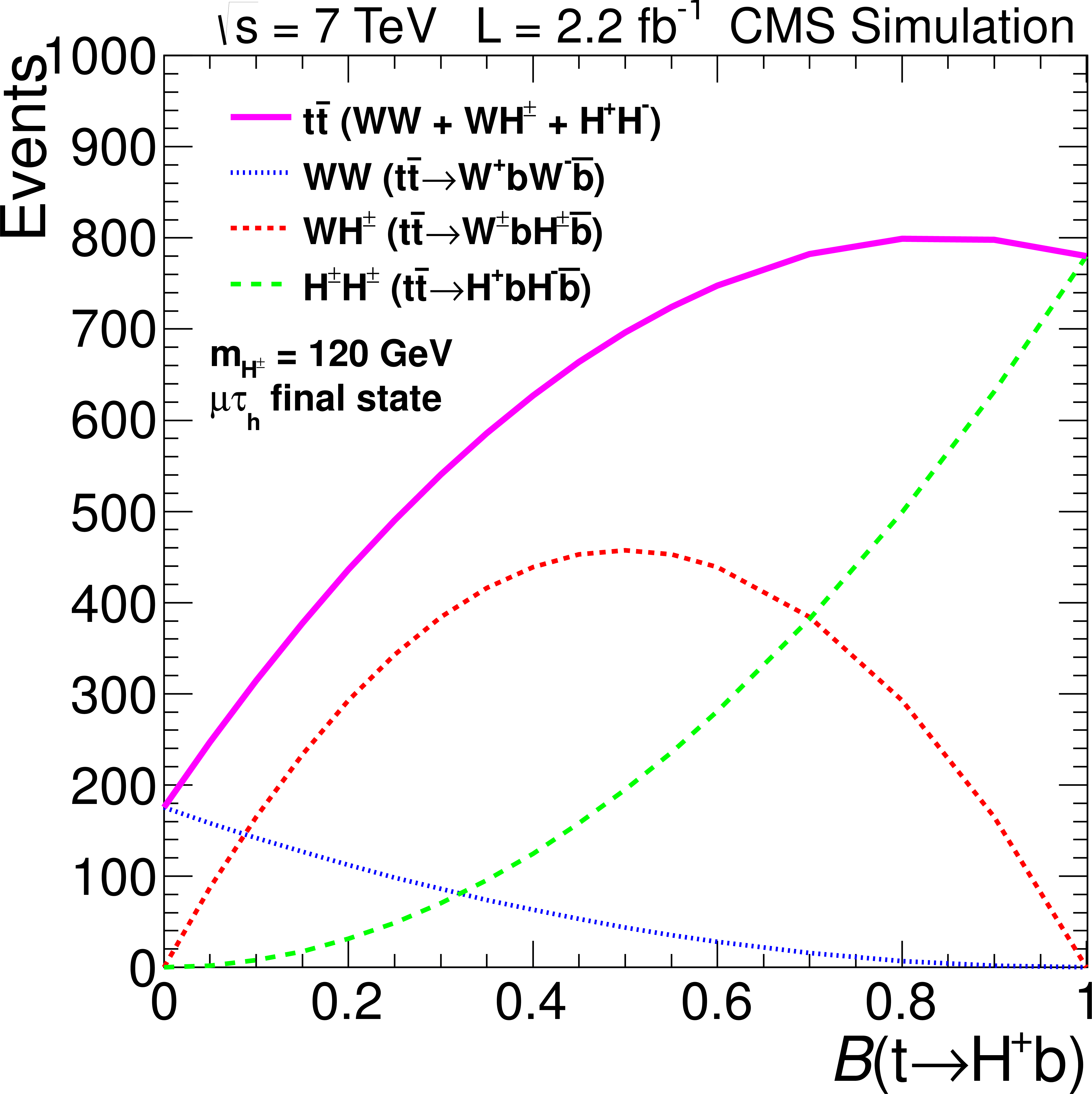
Figure 6-a:
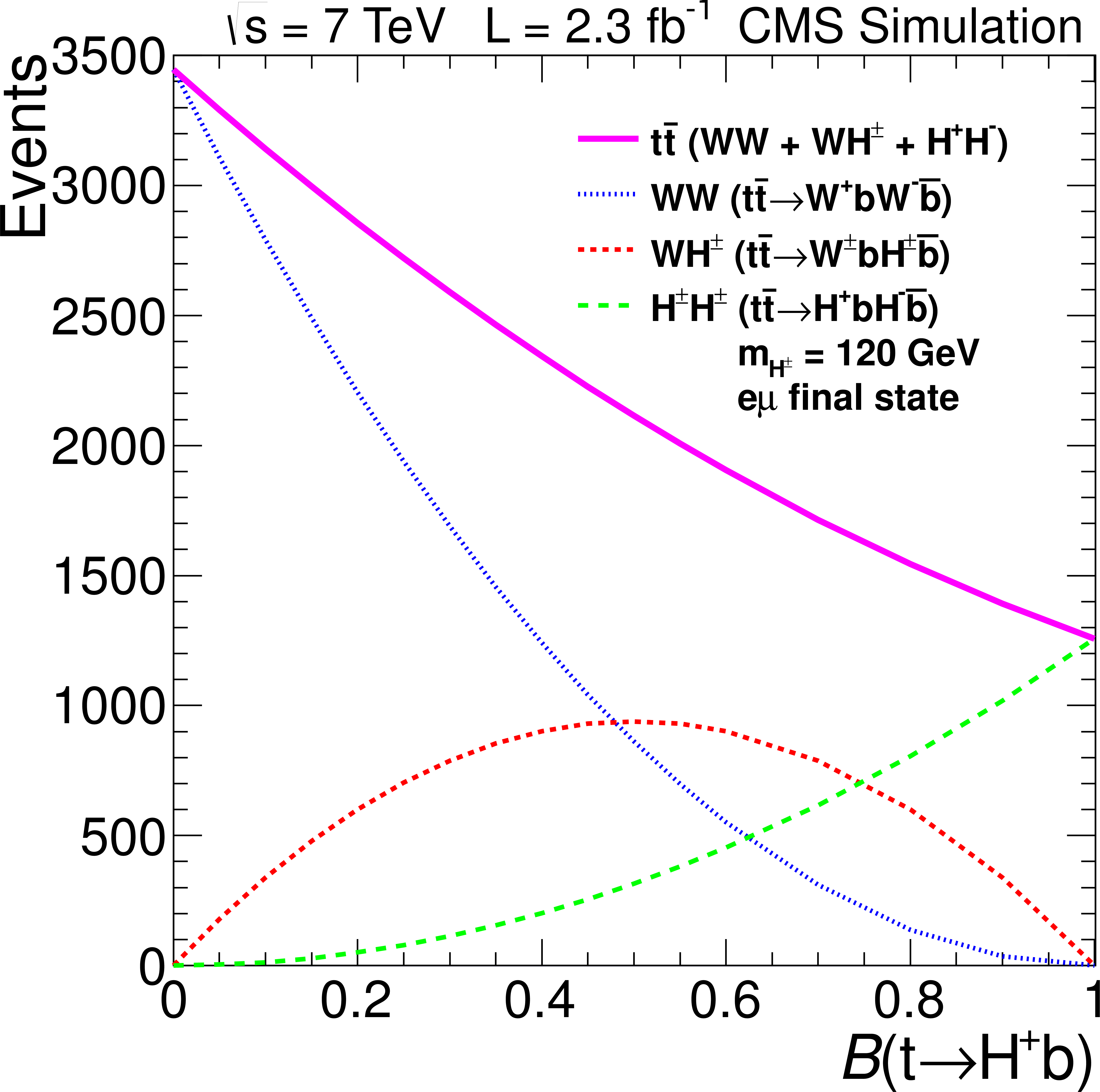
The expected number of $ {\mathrm {t}\overline {\mathrm {t}}} $ events after event selection for the $ {{\mu }} {\tau }_\mathrm {h}$ (a) and $ {\mathrm {e}} {{\mu }}$ (b) final states as a function of the branching fraction $\mathcal {B}( {\mathrm {t}}\rightarrow {\mathrm {H}} ^{+} {\mathrm {b}})$ for $m_{ {\mathrm {H}} ^{+}} =$ 120 GeV. Expectations are shown separately for the $ {\mathrm {W}} {\mathrm {H}} $, $ {\mathrm {H}} {\mathrm {H}} $, and $ {\mathrm {W}} {\mathrm {W}}$ contributions. |
png pdf |
Figure 6-b:
The expected number of $ {\mathrm {t}\overline {\mathrm {t}}} $ events after event selection for the $ {{\mu }} {\tau }_\mathrm {h}$ (a) and $ {\mathrm {e}} {{\mu }}$ (b) final states as a function of the branching fraction $\mathcal {B}( {\mathrm {t}}\rightarrow {\mathrm {H}} ^{+} {\mathrm {b}})$ for $m_{ {\mathrm {H}} ^{+}} =$ 120 GeV. Expectations are shown separately for the $ {\mathrm {W}} {\mathrm {H}} $, $ {\mathrm {H}} {\mathrm {H}} $, and $ {\mathrm {W}} {\mathrm {W}}$ contributions. |

png |
Figure 6:
|
png pdf |
Figure 7-a:
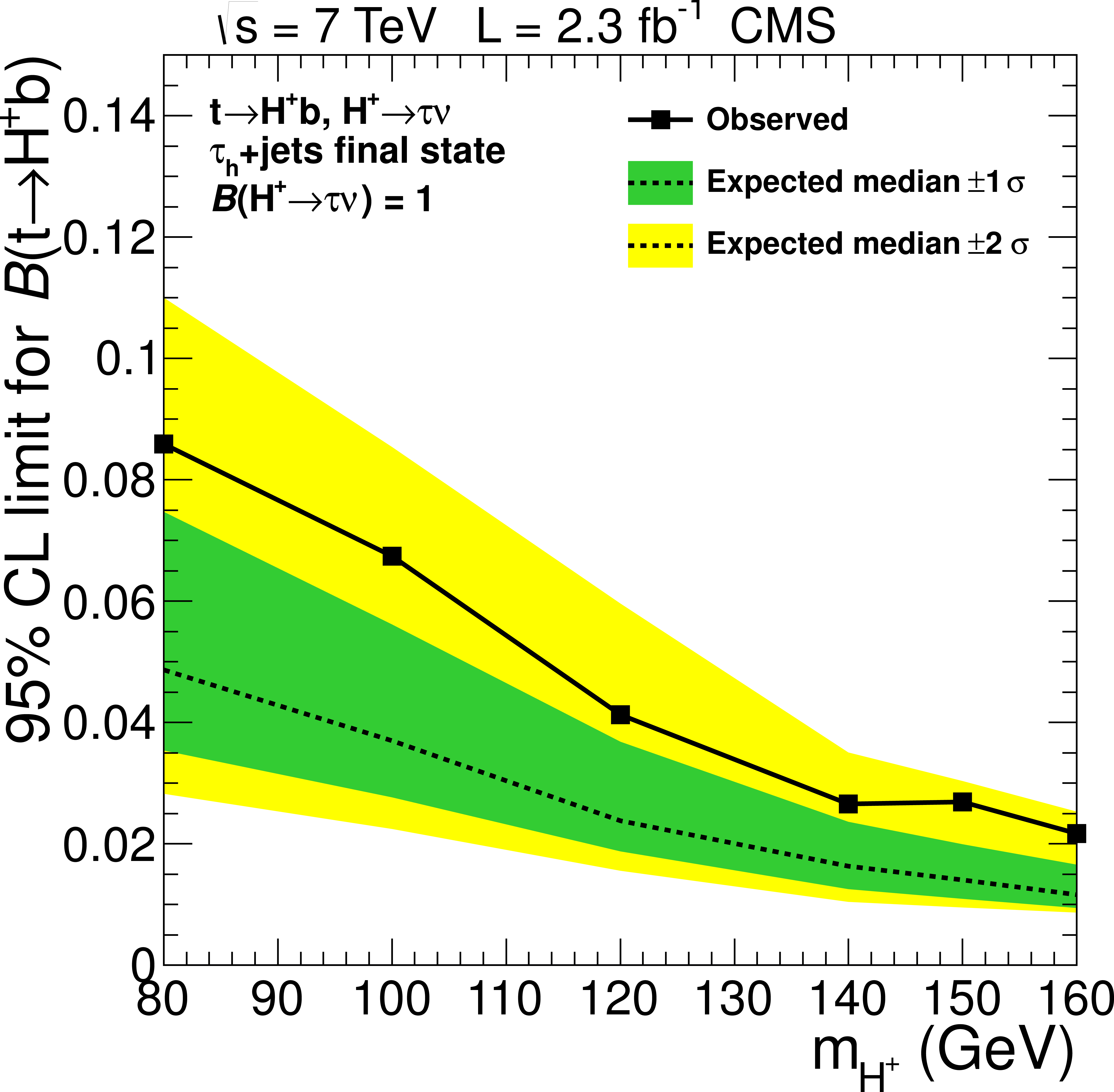
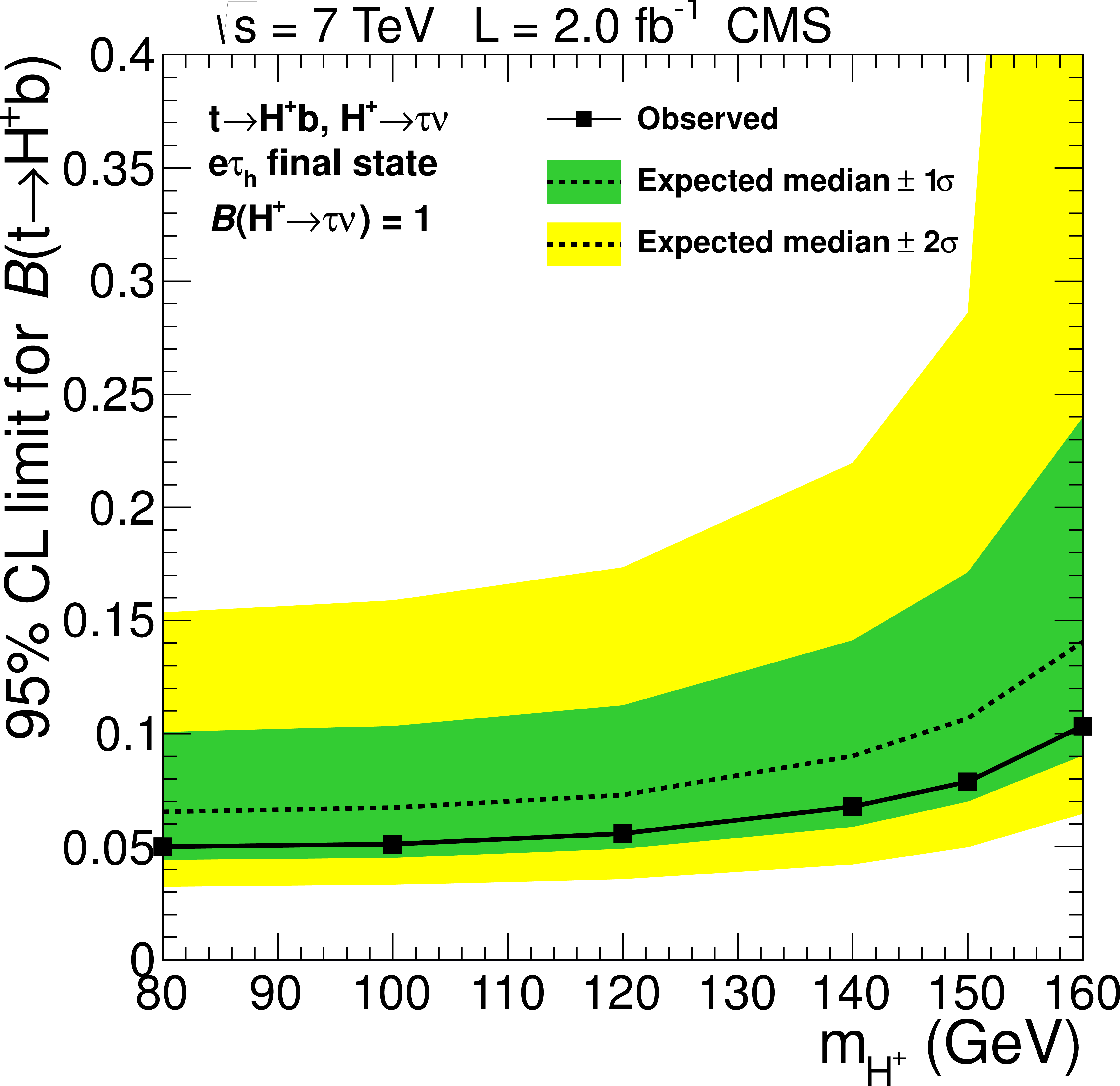
Upper limit on $\mathcal {B}( {\mathrm {t}}\rightarrow {\mathrm {H}} ^{+} {\mathrm {b}})$ as a function of $m_{ {\mathrm {H}} ^{+}}$ for the fully hadronic (a) and the e$ {\tau }_\mathrm {h}$ (b) final states. The $\pm 1 \sigma $ and $\pm 2 \sigma $ bands around the expected limit are also shown. |
png pdf |
Figure 7-b:
Upper limit on $\mathcal {B}( {\mathrm {t}}\rightarrow {\mathrm {H}} ^{+} {\mathrm {b}})$ as a function of $m_{ {\mathrm {H}} ^{+}}$ for the fully hadronic (a) and the e$ {\tau }_\mathrm {h}$ (b) final states. The $\pm 1 \sigma $ and $\pm 2 \sigma $ bands around the expected limit are also shown. |

png |
Figure 7:
|
png pdf |
Figure 8-a:
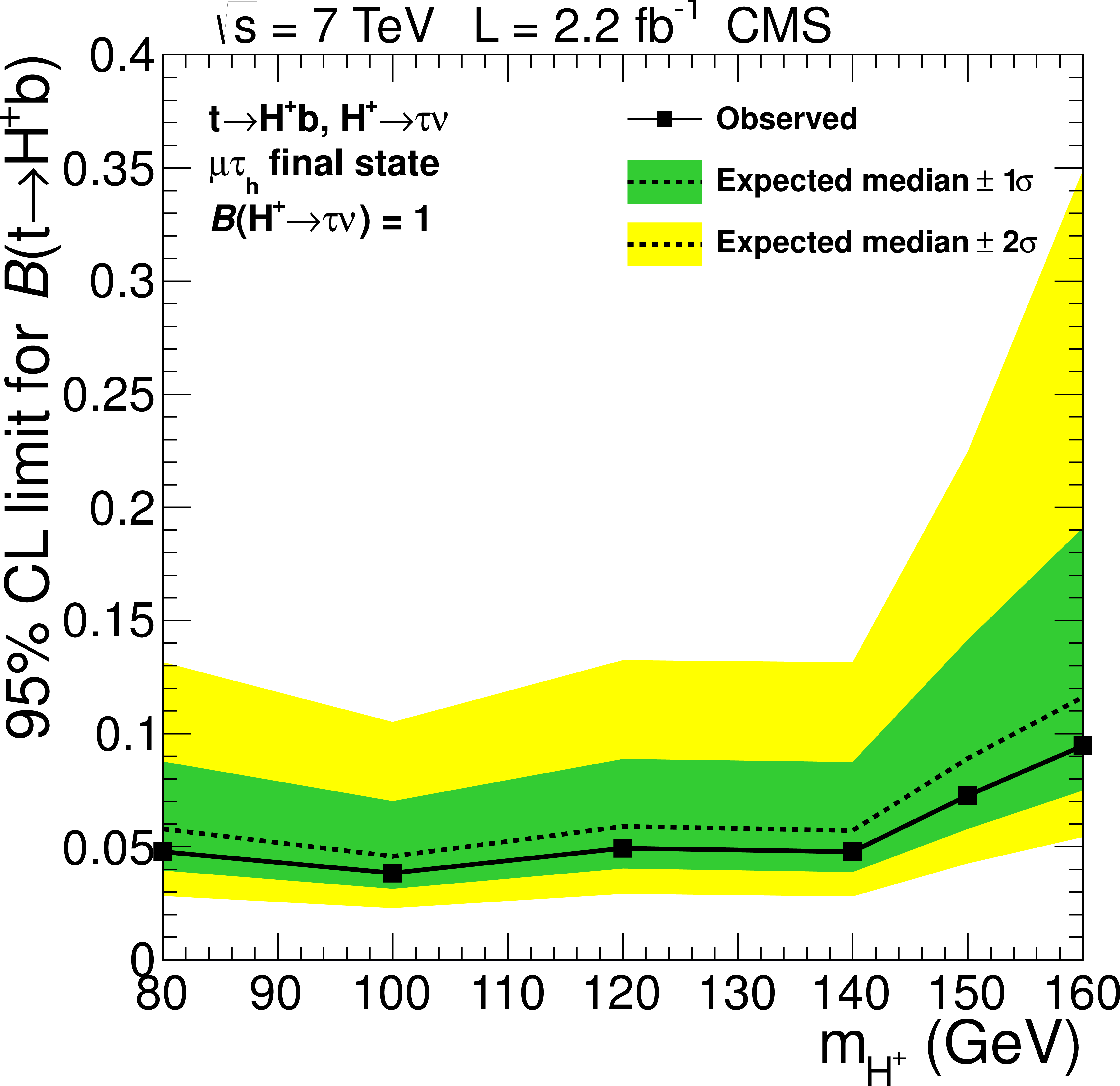
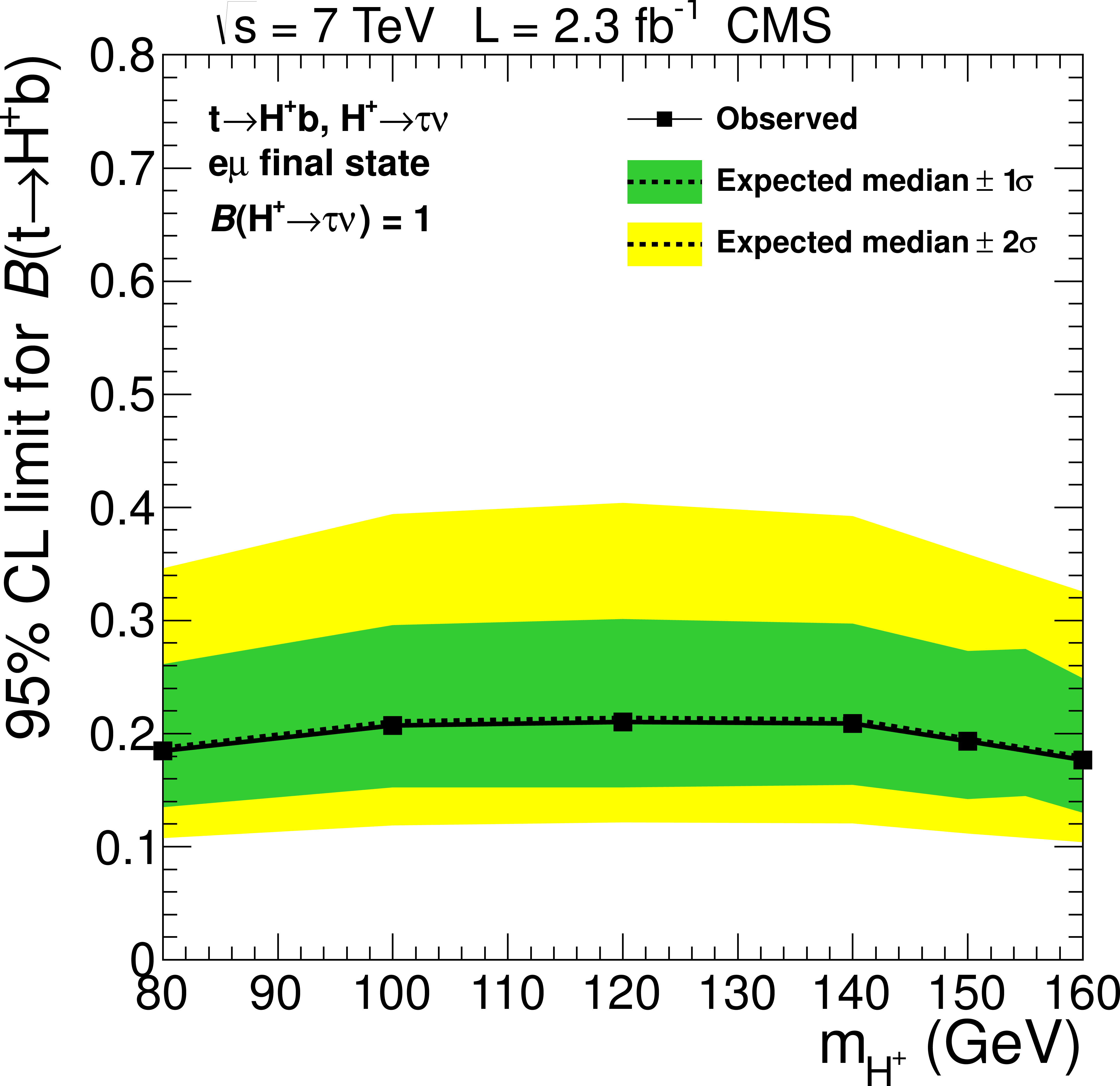
Upper limit on $\mathcal {B}( {\mathrm {t}}\rightarrow {\mathrm {H}} ^{+} {\mathrm {b}})$ as a function of $m_{ {\mathrm {H}} ^{+}}$ for the $ {{\mu }} {\tau }_\mathrm {h}$ (a) and $ {\mathrm {e}} {{\mu }}$ (b) final states. The $\pm 1 \sigma $ and $\pm 2 \sigma $ bands around the expected limit are also shown. |
png pdf |
Figure 8-b:
Upper limit on $\mathcal {B}( {\mathrm {t}}\rightarrow {\mathrm {H}} ^{+} {\mathrm {b}})$ as a function of $m_{ {\mathrm {H}} ^{+}}$ for the $ {{\mu }} {\tau }_\mathrm {h}$ (a) and $ {\mathrm {e}} {{\mu }}$ (b) final states. The $\pm 1 \sigma $ and $\pm 2 \sigma $ bands around the expected limit are also shown. |

png |
Figure 8:
|
png pdf |
Figure 9-a:
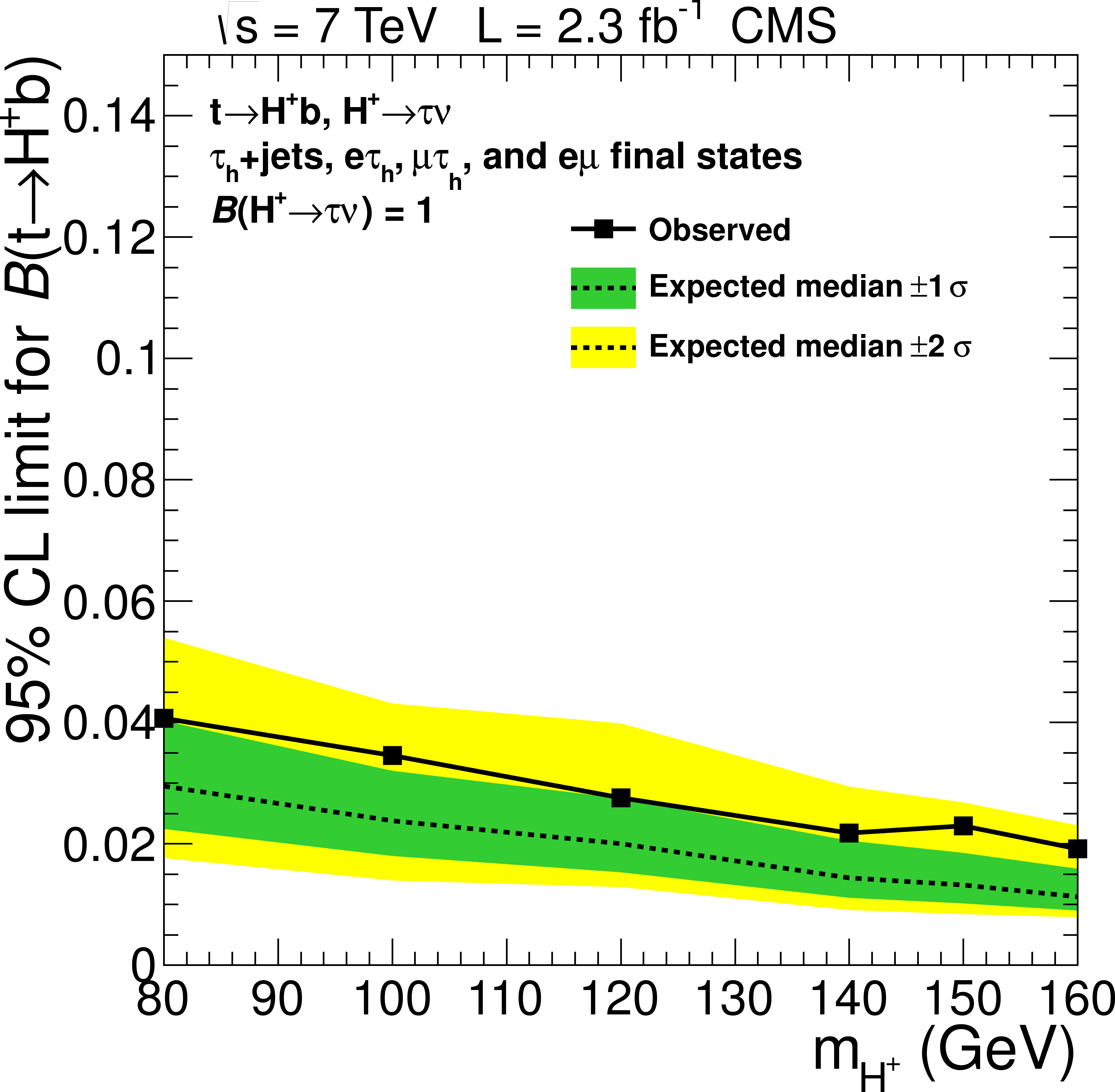
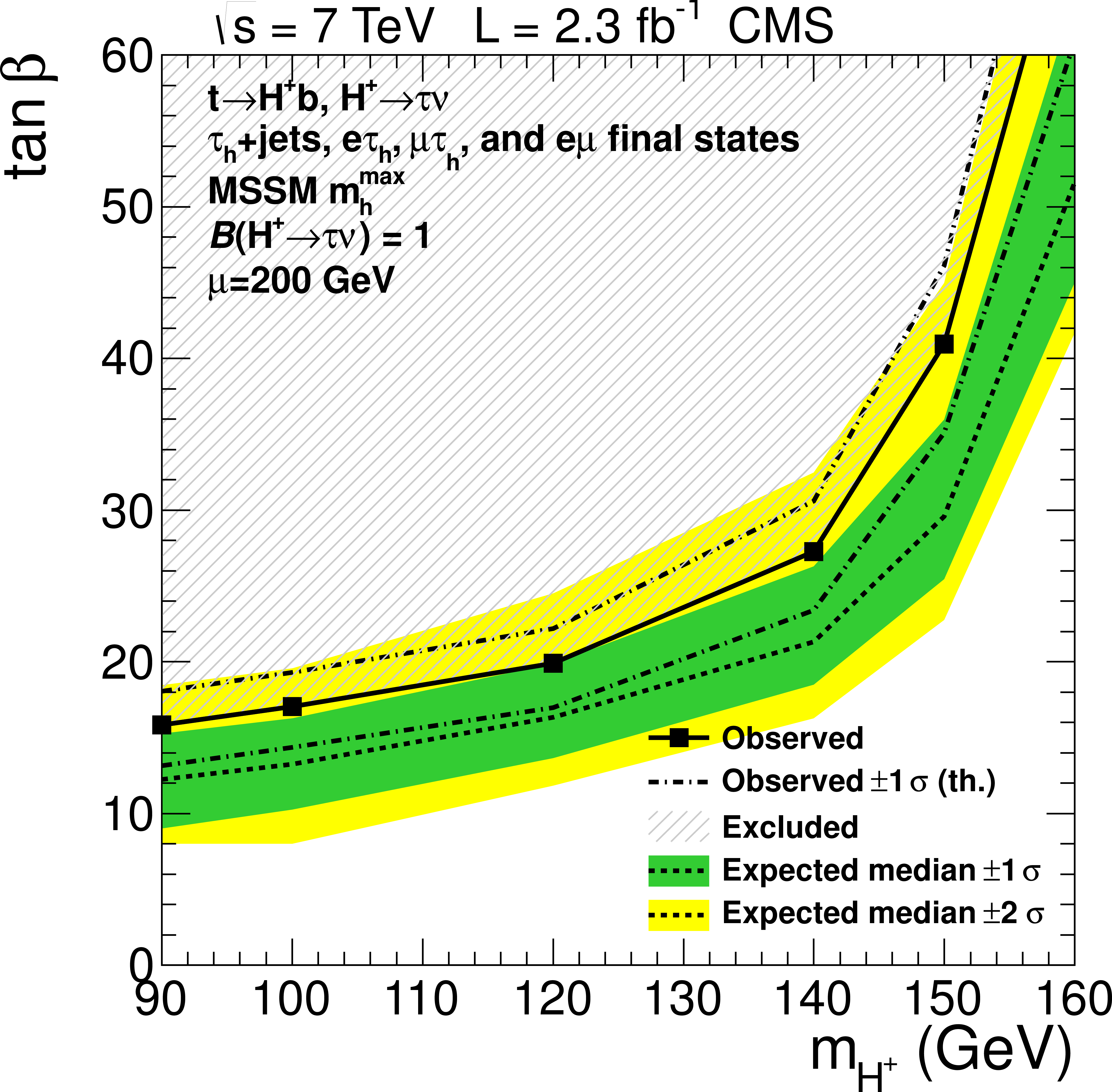
a: the upper limit on $\mathcal {B}( {\mathrm {t}}\rightarrow {\mathrm {H}} ^{+} {\mathrm {b}})$ as a function of $m_{ {\mathrm {H}} ^{+}}$ obtained from the combination of the all final states. b: the exclusion region in the MSSM $M_{ {\mathrm {H}} ^{+}}$-$\tan\beta $ parameter space obtained from the combined analysis for the MSSM $m_\mathrm {h}^\text {max}$ scenario. The $\pm 1 \sigma $ and $\pm 2 \sigma $ bands around the expected limit are also shown. |
png pdf |
Figure 9-b:
a: the upper limit on $\mathcal {B}( {\mathrm {t}}\rightarrow {\mathrm {H}} ^{+} {\mathrm {b}})$ as a function of $m_{ {\mathrm {H}} ^{+}}$ obtained from the combination of the all final states. b: the exclusion region in the MSSM $M_{ {\mathrm {H}} ^{+}}$-$\tan\beta $ parameter space obtained from the combined analysis for the MSSM $m_\mathrm {h}^\text {max}$ scenario. The $\pm 1 \sigma $ and $\pm 2 \sigma $ bands around the expected limit are also shown. |

png |
Figure 9:
|
| Tables | |
png pdf |
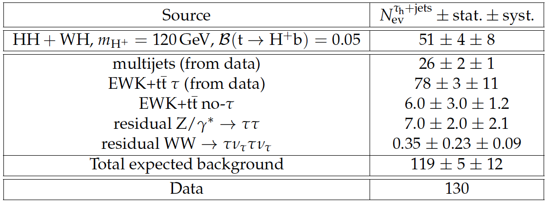
Table 1:
Numbers of expected events in the $ {\tau }_\mathrm {h}$+jets analysis for the backgrounds and the Higgs boson signal from $ {\mathrm {H}} {\mathrm {H}} $ and $ {\mathrm {W}} {\mathrm {H}} $ processes at $m_{ {\mathrm {H}} ^{+}} =$ 120 GeV, and the number of observed events after the final event selection. Unless stated differently, the expected background events are from simulation. |
png pdf |
Table 2:
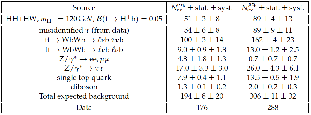
Numbers of expected events in the $ {\mathrm {e}} {\tau }_\mathrm {h}$ and $\mu {\tau }_\mathrm {h}$ analyses for the backgrounds and the Higgs boson signal from $ {\mathrm {W}} {\mathrm {H}} $ and $ {\mathrm {H}} {\mathrm {H}} $ processes at $m_{ {\mathrm {H}} ^{+}} =$ 120 GeV, and the number of observed events after the final event selection. Unless stated differently, the expected background events are from simulation. |

png pdf |
Table 3:
Number of expected events in the $ {\mathrm {e}} {{\mu }}$ analysis for the backgrounds, the Higgs boson signal from $ {\mathrm {H}} {\mathrm {H}} $ and $ {\mathrm {W}} {\mathrm {H}} $ processes at $m_{ {\mathrm {H}} ^{+}}=$ 120 GeV, and the number of observed events after all selection requirements. The expected background events are from simulation. |
png pdf |
Table 4:
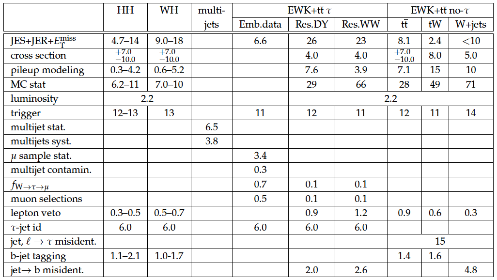
The systematic uncertainties on event yields (in percent) for the $ {\tau }_\mathrm {h}$+jets analysis for background processes and for the Higgs boson signal processes $ {\mathrm {W}} {\mathrm {H}} $ and $ {\mathrm {H}} {\mathrm {H}} $ in the range of $m_{ {\mathrm {H}} ^{+}} =$ 80-160 GeV. The range of errors for the signal processes is given for the Higgs boson mass range of 80-160 GeV. |
png pdf |
Table 5:
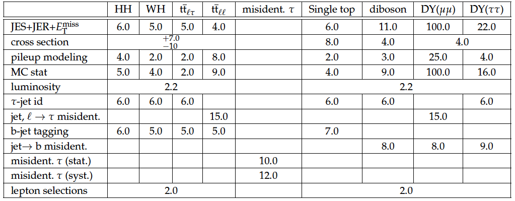
The systematic uncertainties on event yields (in percent) for the $ {{\mu }} {\tau }_\mathrm {h}$ analysis for the background processes and for the Higgs boson signal processes $ {\mathrm {W}} {\mathrm {H}} $ and $ {\mathrm {H}} {\mathrm {H}} $ for $m_{ {\mathrm {H}} ^{+}} =$ 120 GeV. |
png pdf |
Table 6:
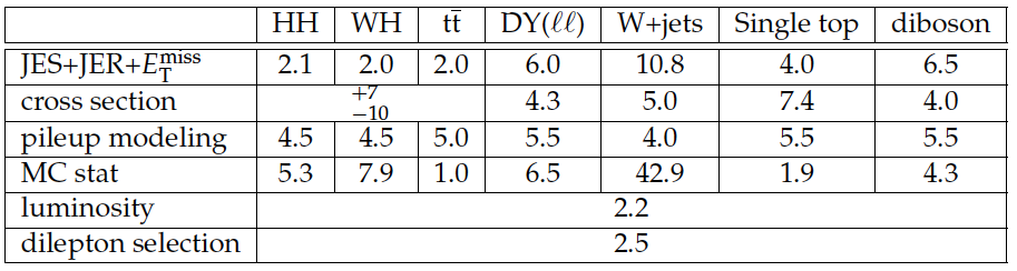
The systematic uncertainties on event yields (in percent) for the $ {\mathrm {e}} {{\mu }}$ analysis for the background processes and for the Higgs boson signal processes $ {\mathrm {W}} {\mathrm {H}} $ and $ {\mathrm {H}} {\mathrm {H}} $ at $m_{ {\mathrm {H}} ^{+}} =$ 120 GeV. |
png pdf |
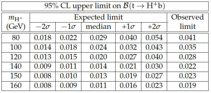
Table 7:
The expected range and observed 95% CL upper limit for $\mathcal {B}( {\mathrm {t}}\rightarrow {\mathrm {H}} ^{+} {\mathrm {b}})$ as a function of $m_{ {\mathrm {H}} ^{+}}$ for the combination of the fully hadronic, $ {\mathrm {e}} {\tau }_\mathrm {h}$, $ {{\mu }} {\tau }_\mathrm {h}$, and $ {\mathrm {e}} {{\mu }}$ final states. |
|
|
Compact Muon Solenoid LHC, CERN |
|

|

|

|

|

|