CMS-HIG-13-002

CMS-HIG-13-002 ; CERN-PH-EP-2013-220
Measurement of the properties of a Higgs boson in the four-lepton final state
CMS Collaboration
19 December 2013
Phys. Rev. D 89 (2014) 092007
Abstract: The properties of a Higgs boson candidate are measured in the $ \mathrm{H} \to \mathrm{ZZ} \to 4\ell$ decay channel, with $ \ell = \mathrm{e},\, \mu $, using data from pp collisions corresponding to an integrated luminosity of 5.1 fb$ ^{-1} $ at center-of-mass energy of $\sqrt{s}$ = 7 TeV and 19.7 fm$ ^{-1} $ at $ \sqrt{s} $ = 8 TeV, recorded with the CMS detector at the LHC. The new boson is observed as a narrow resonance with a local significance of 6.8 standard deviations, a measured mass of 125.6 $ \pm $ 0.4 (stat.) $ \pm $ 0.2 (syst.) GeV, and a total width less than 3.4 GeV at a 95% confidence level. The production cross section of the new boson times the branching fraction to four leptons is measured to be 0.93$ ^{+0.26}_{-0.23}$ (stat.) $^{+0.13}_{-0.09}$ (syst.) times that predicted by the standard model. Its spin-parity properties are found to be consistent with the expectations for the standard model Higgs boson. The hypotheses of a pseudoscalar and all tested spin-one boson hypotheses are excluded at a 99% confidence level or higher. All tested spin-two boson hypotheses are excluded at a 95% confidence level or higher.
Links: e-print arXiv:1312.5353 [hep-ex] (PDF) ; CDS record ; inSPIRE record ; Public twiki page ; CADI line (restricted) ;

Figures	CMS Publications

Figures
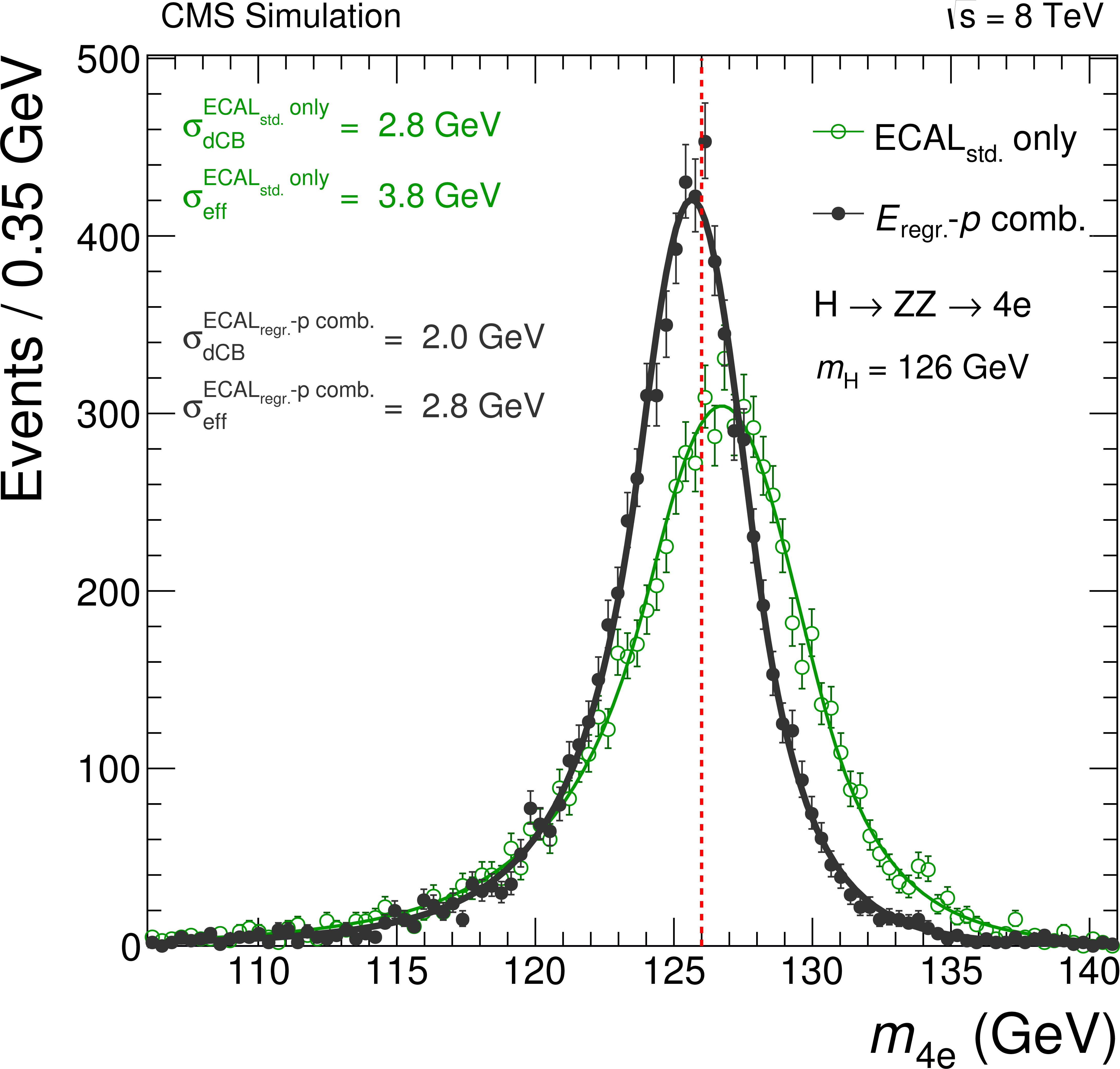
png pdf	Figure 1-a: (a) Expected four-lepton mass distribution for $ {\mathrm {H}} \to {\mathrm {Z}} {\mathrm {Z}}\to 4 {\mathrm {e}}$ for $ {m_{ {\mathrm {H}} }} $ = 126 GeV using ECAL-only electron momentum estimation (green open points: $\mathrm {ECAL}_\text {std.}$ only), and using the method employed in this analysis (black full points: $E_\text {regr}-p$ combination). The fitted standard deviation, $\sigma _\mathrm {dCB}$, of the double-sided Crystal-Ball function and effective width $\sigma _\text {eff}$ defined in the text are indicated. Electrons with $ {p_{\mathrm {T}}} ^ {\mathrm {e}}> 7$ GeV in the full $\eta ^ {\mathrm {e}}$ range are used. (b) Expected effective momentum resolution $\sigma _\text {eff}/p$ for electrons in the EB as a function of the momentum for the ECAL-only, the tracker-only, and the combined estimates.
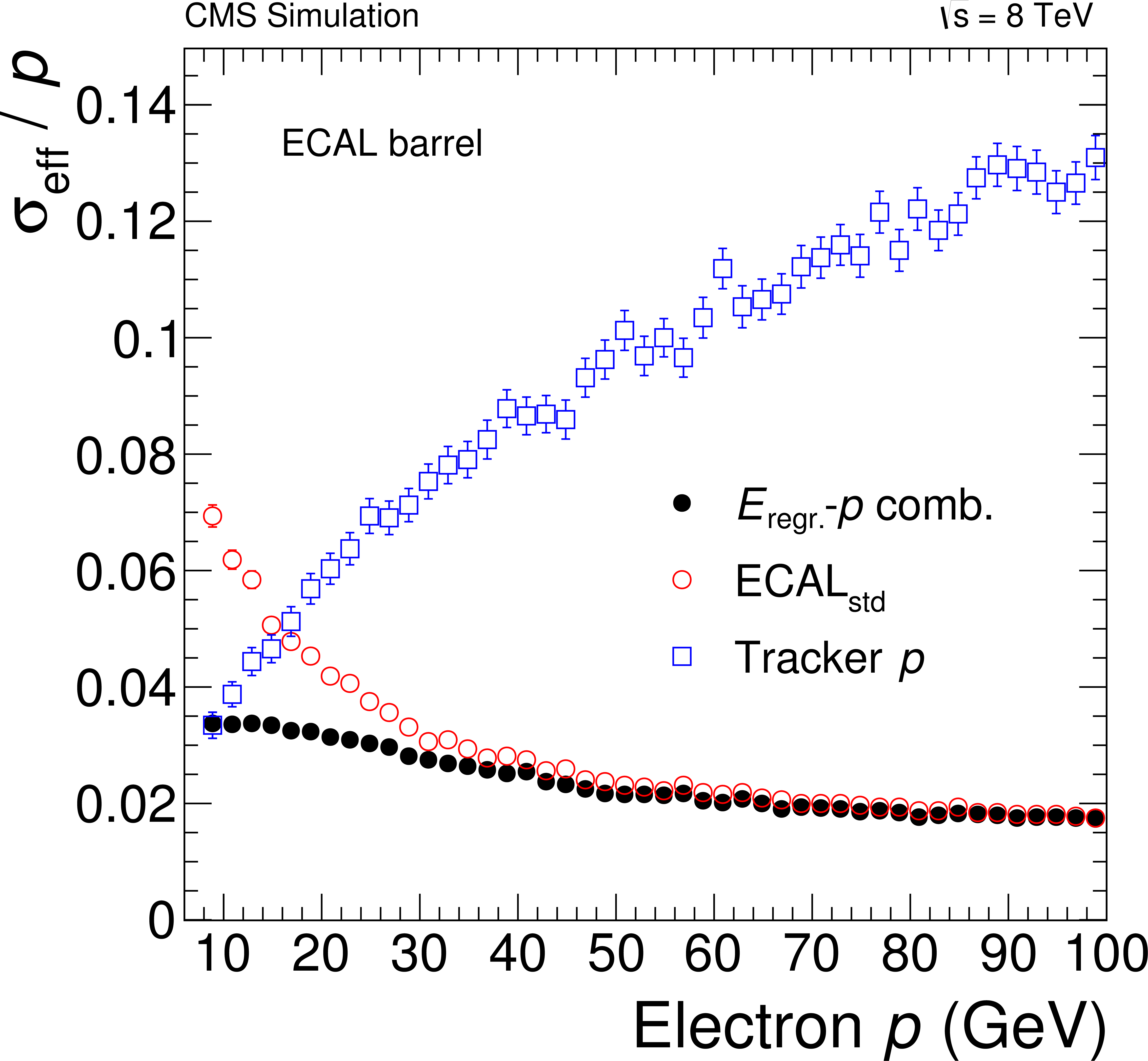
png pdf	Figure 1-b: (a) Expected four-lepton mass distribution for $ {\mathrm {H}} \to {\mathrm {Z}} {\mathrm {Z}}\to 4 {\mathrm {e}}$ for $ {m_{ {\mathrm {H}} }} $ = 126 GeV using ECAL-only electron momentum estimation (green open points: $\mathrm {ECAL}_\text {std.}$ only), and using the method employed in this analysis (black full points: $E_\text {regr}-p$ combination). The fitted standard deviation, $\sigma _\mathrm {dCB}$, of the double-sided Crystal-Ball function and effective width $\sigma _\text {eff}$ defined in the text are indicated. Electrons with $ {p_{\mathrm {T}}} ^ {\mathrm {e}}> 7$ GeV in the full $\eta ^ {\mathrm {e}}$ range are used. (b) Expected effective momentum resolution $\sigma _\text {eff}/p$ for electrons in the EB as a function of the momentum for the ECAL-only, the tracker-only, and the combined estimates.
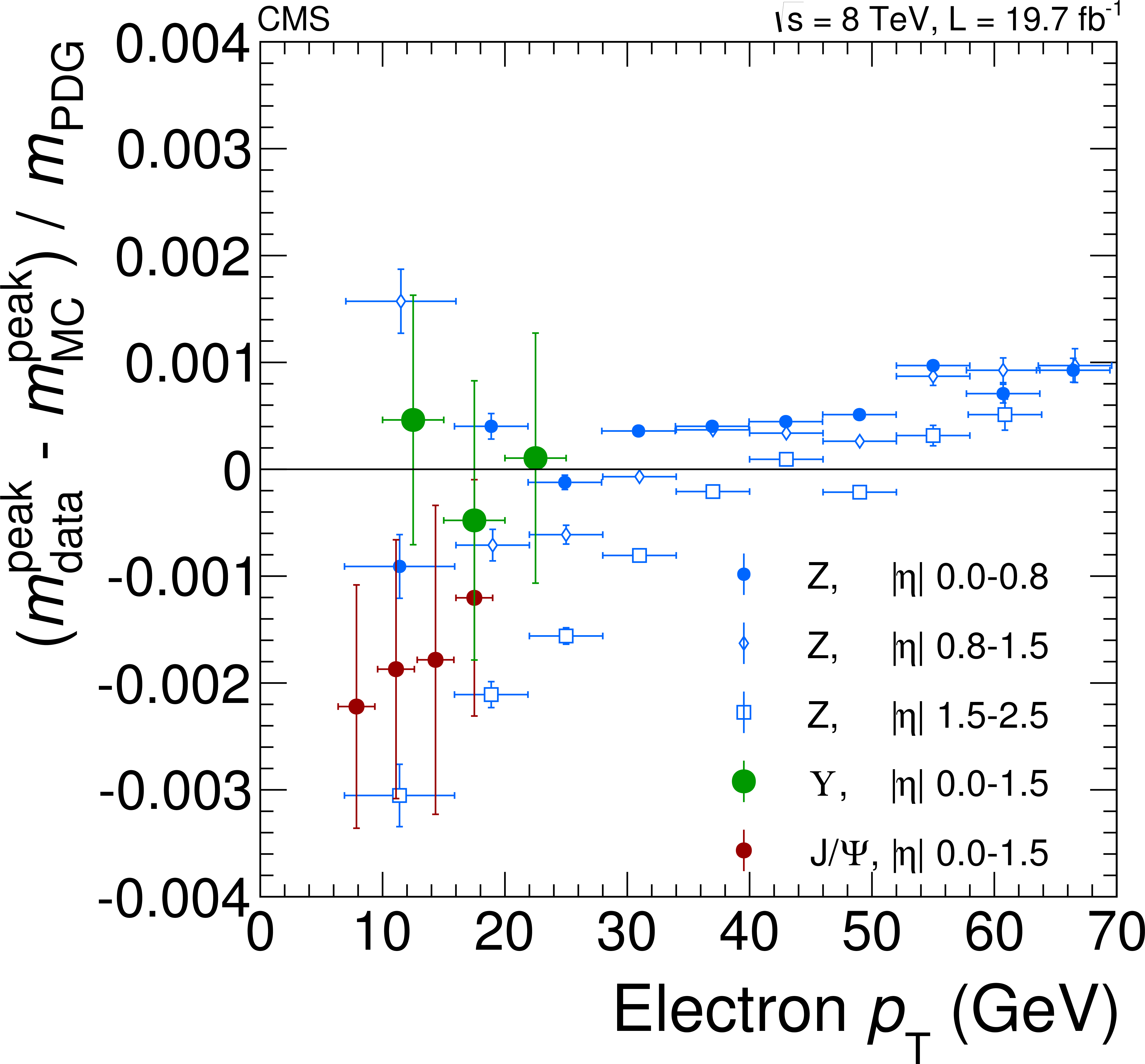
png pdf	Figure 2-a: Relative difference between the dilepton mass peak positions in data and simulation as obtained from $ {\mathrm {Z}}$, $ {\mathrm {J} / \psi } $ and $ { {\Upsilon }(\mathrm {nS})}$ resonances as a function of (left) the transverse momentum of one of the electrons regardless of the second for dielectron events, and (right) the average muon $ {p_{\mathrm {T}}} ^ {{\mu }}$ for dimuon events for the 8 TeV data.
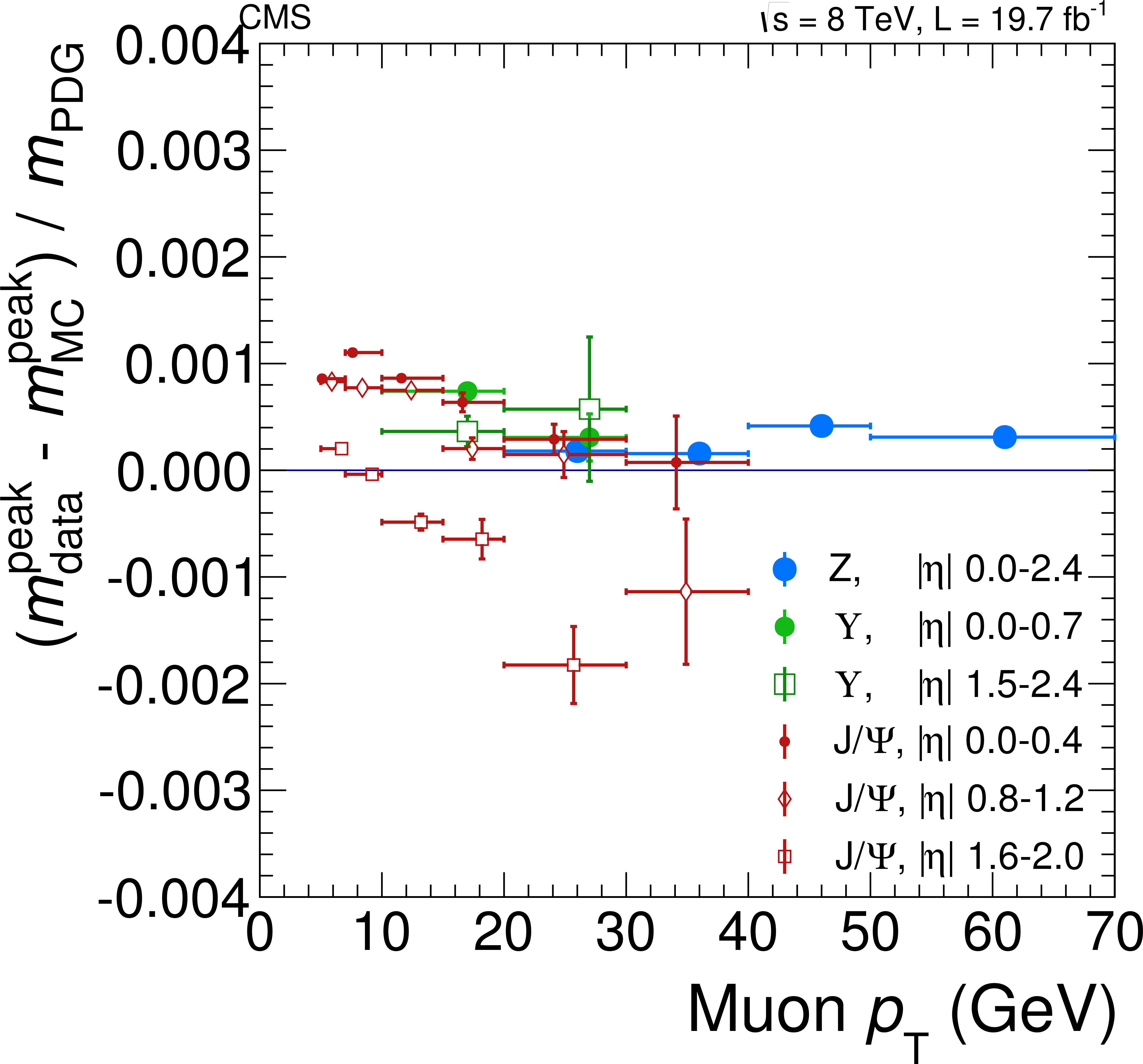
png pdf	Figure 2-b: Relative difference between the dilepton mass peak positions in data and simulation as obtained from $ {\mathrm {Z}}$, $ {\mathrm {J} / \psi } $ and $ { {\Upsilon }(\mathrm {nS})}$ resonances as a function of (left) the transverse momentum of one of the electrons regardless of the second for dielectron events, and (right) the average muon $ {p_{\mathrm {T}}} ^ {{\mu }}$ for dimuon events for the 8 TeV data.
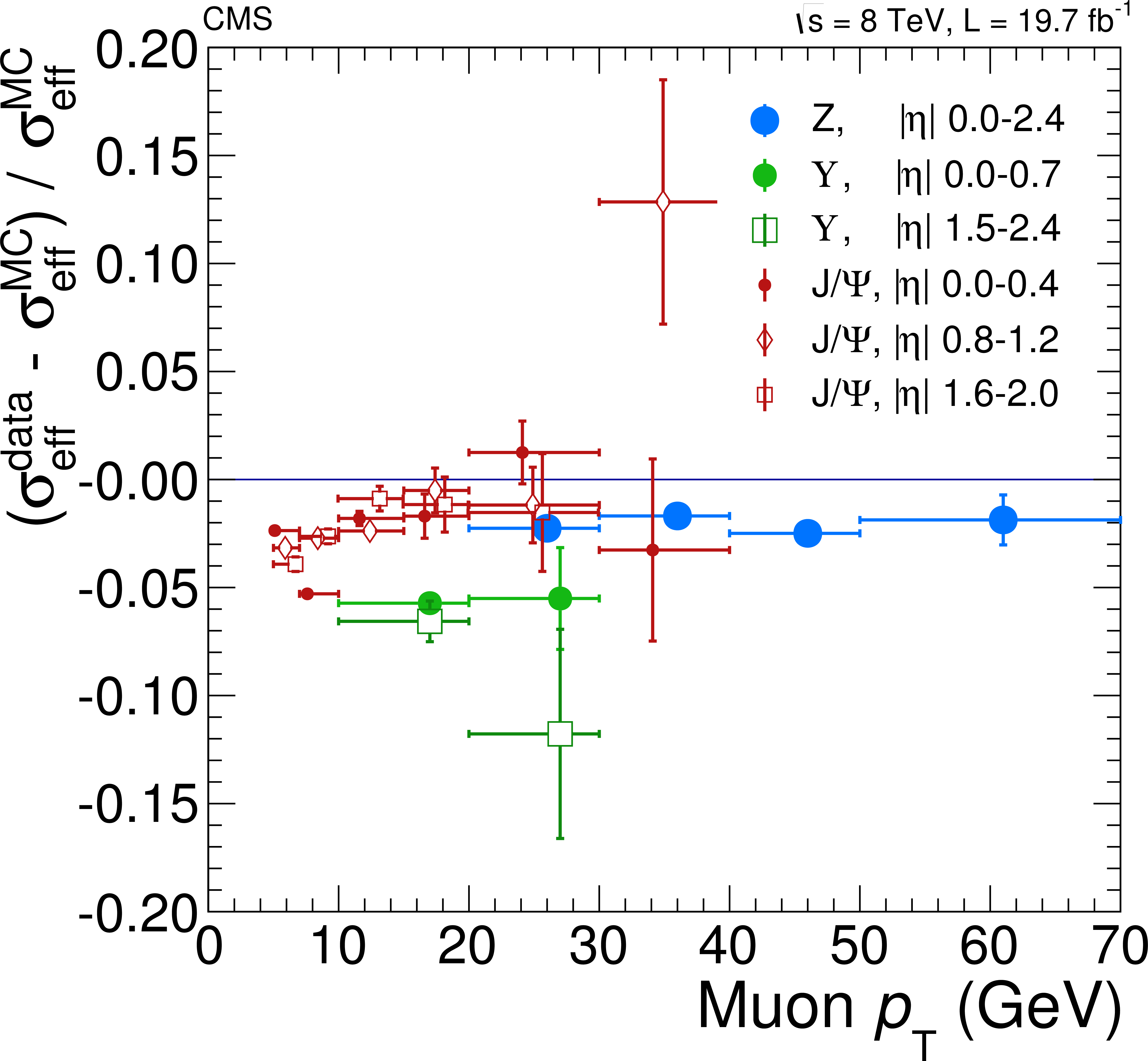
png pdf	Figure 3-a: (a) Relative difference between the dielectron $\sigma _\text {eff}$ in data and simulation, as measured from $ {\mathrm {Z}}\to {\mathrm {e}^+} {\mathrm {e}^-}$ events, where the electrons are classified into different categories (B: barrel, E: end caps, G: golden, S: showering). (b) Relative difference between the dimuon mass resolutions in data and simulation as measured from $ {\mathrm {J} / \psi } $, $ { {\Upsilon }(\mathrm {nS})}$, and $ {\mathrm {Z}}$ decays as functions of the average muon $ {p_{\mathrm {T}}} ^ {{\mu }}$. The uncertainties shown are statistical only. Results are presented for data collected at $\sqrt {s}= 8$ TeV .
png pdf	Figure 3-b: (a) Relative difference between the dielectron $\sigma _\text {eff}$ in data and simulation, as measured from $ {\mathrm {Z}}\to {\mathrm {e}^+} {\mathrm {e}^-}$ events, where the electrons are classified into different categories (B: barrel, E: end caps, G: golden, S: showering). (b) Relative difference between the dimuon mass resolutions in data and simulation as measured from $ {\mathrm {J} / \psi } $, $ { {\Upsilon }(\mathrm {nS})}$, and $ {\mathrm {Z}}$ decays as functions of the average muon $ {p_{\mathrm {T}}} ^ {{\mu }}$. The uncertainties shown are statistical only. Results are presented for data collected at $\sqrt {s}= 8$ TeV .
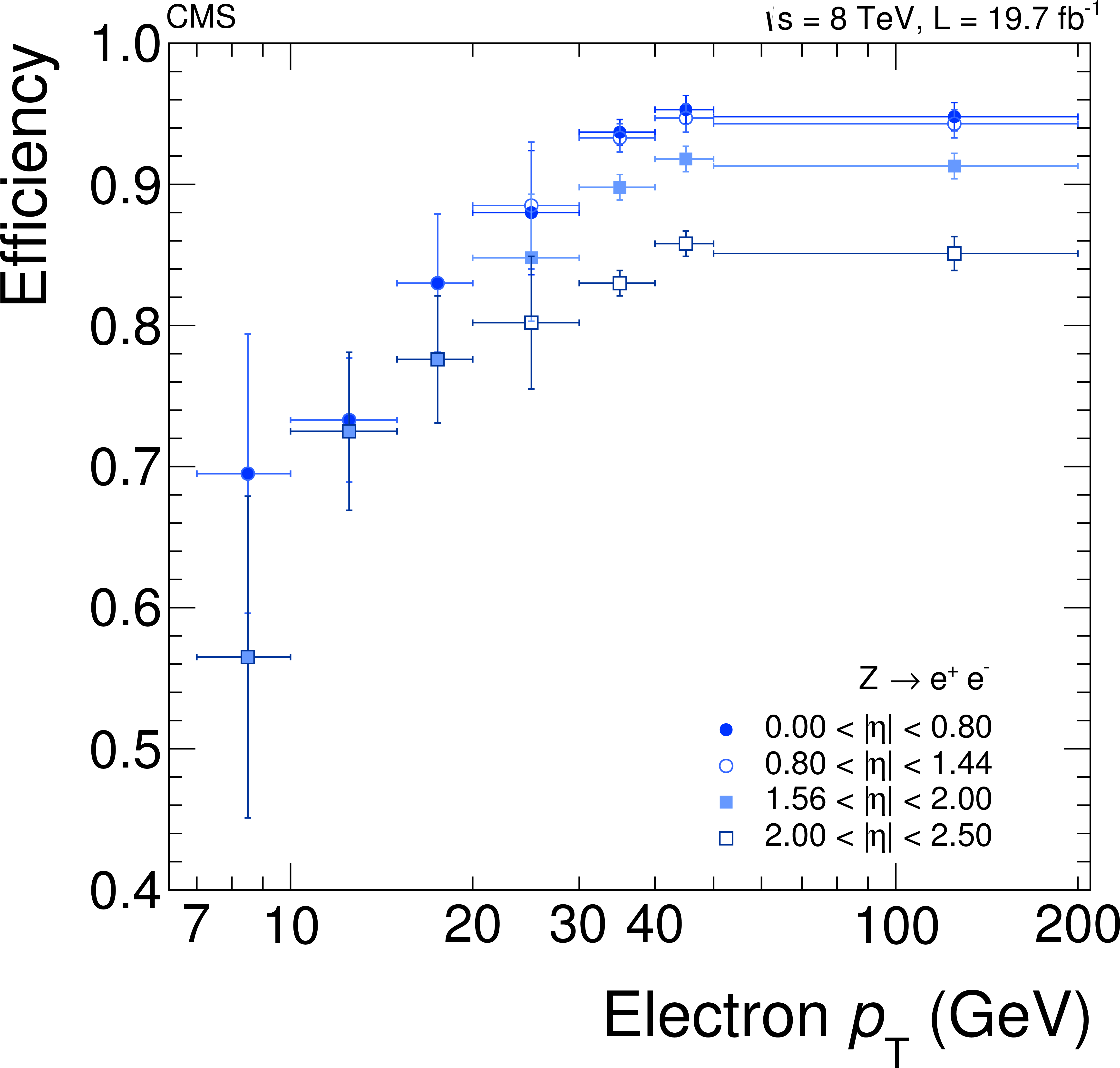
png pdf	Figure 4-a: Efficiency, as a function of the lepton $ {p_{\mathrm {T}}} ^\ell $, for reconstructing and selecting (a) electrons and (b) muons, measured with a $ {\mathrm {Z}}\to \ell \ell $ data sample by using a tag-and-probe method.
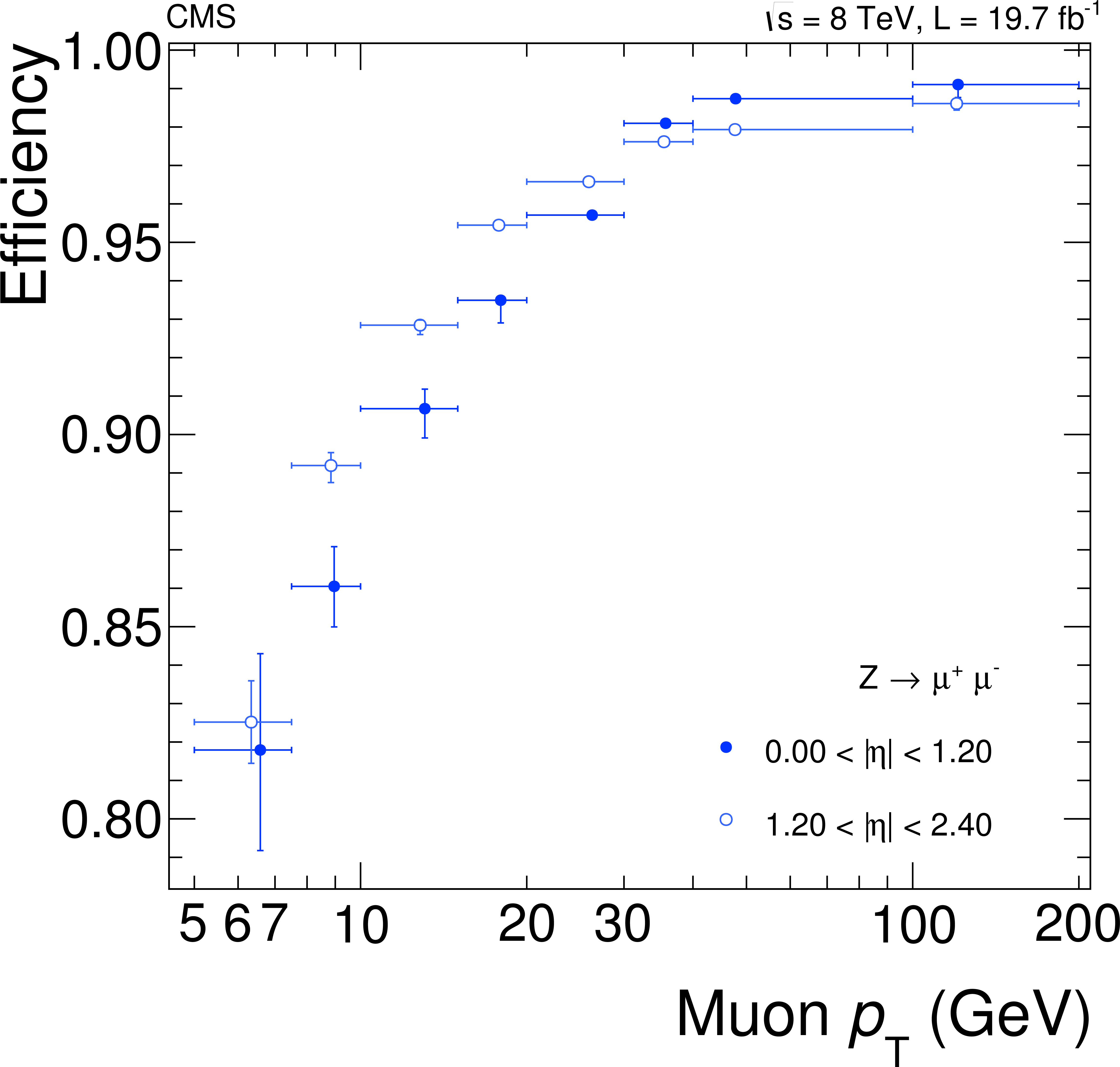
png pdf	Figure 4-b: Efficiency, as a function of the lepton $ {p_{\mathrm {T}}} ^\ell $, for reconstructing and selecting (a) electrons and (b) muons, measured with a $ {\mathrm {Z}}\to \ell \ell $ data sample by using a tag-and-probe method.
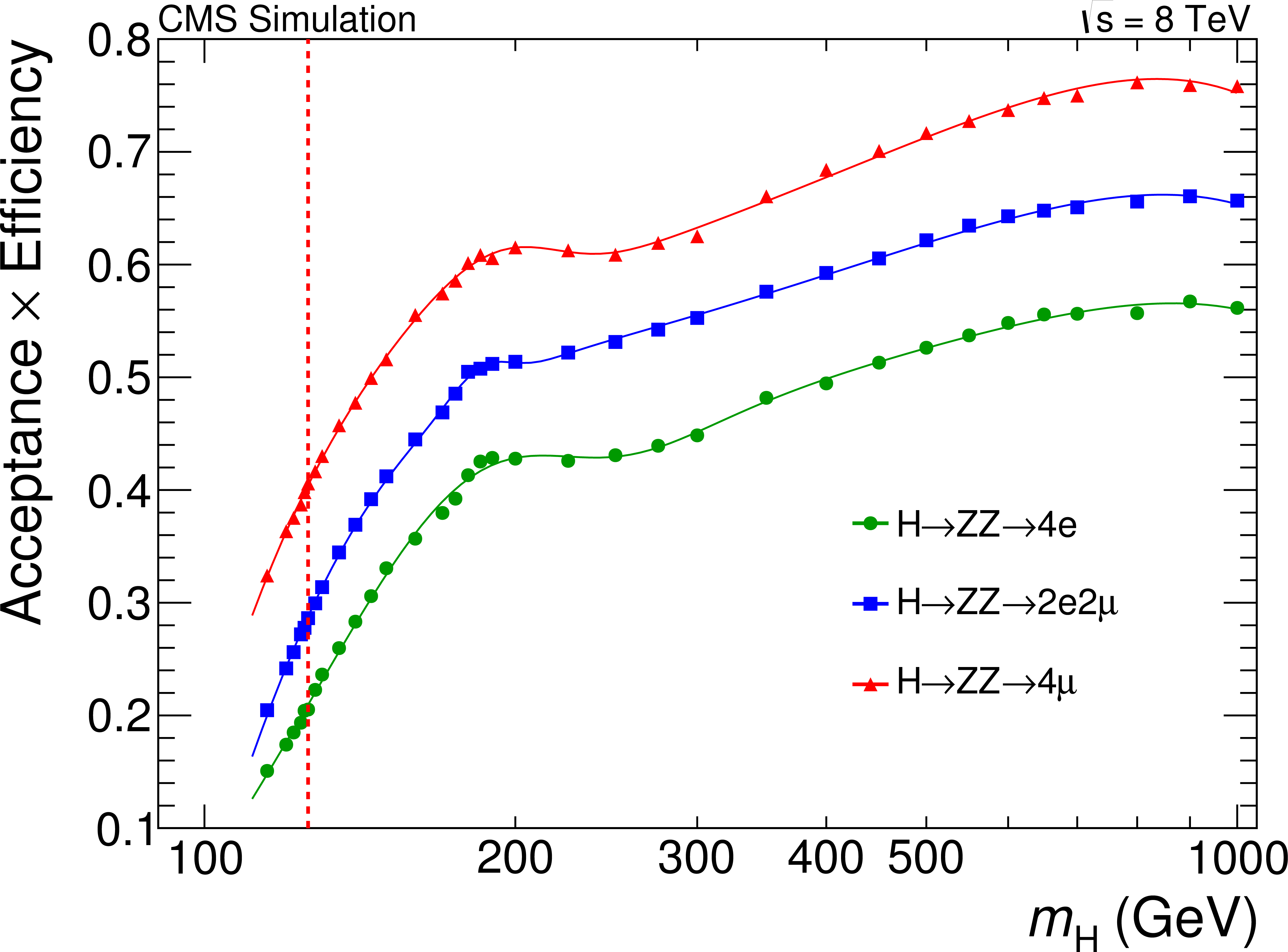
png pdf	Figure 5: Geometrical acceptance times selection efficiency for the SM Higgs boson signal as a function of $ {m_{ {\mathrm {H}} }}$ in the three final states for gluon fusion production. Points represent efficiency estimated from full CMS simulation; lines represent a smooth polynomial curve interpolating the points, used in the analysis. The vertical dashed line represents $ {m_{ {\mathrm {H}} }} $ = 126 GeV
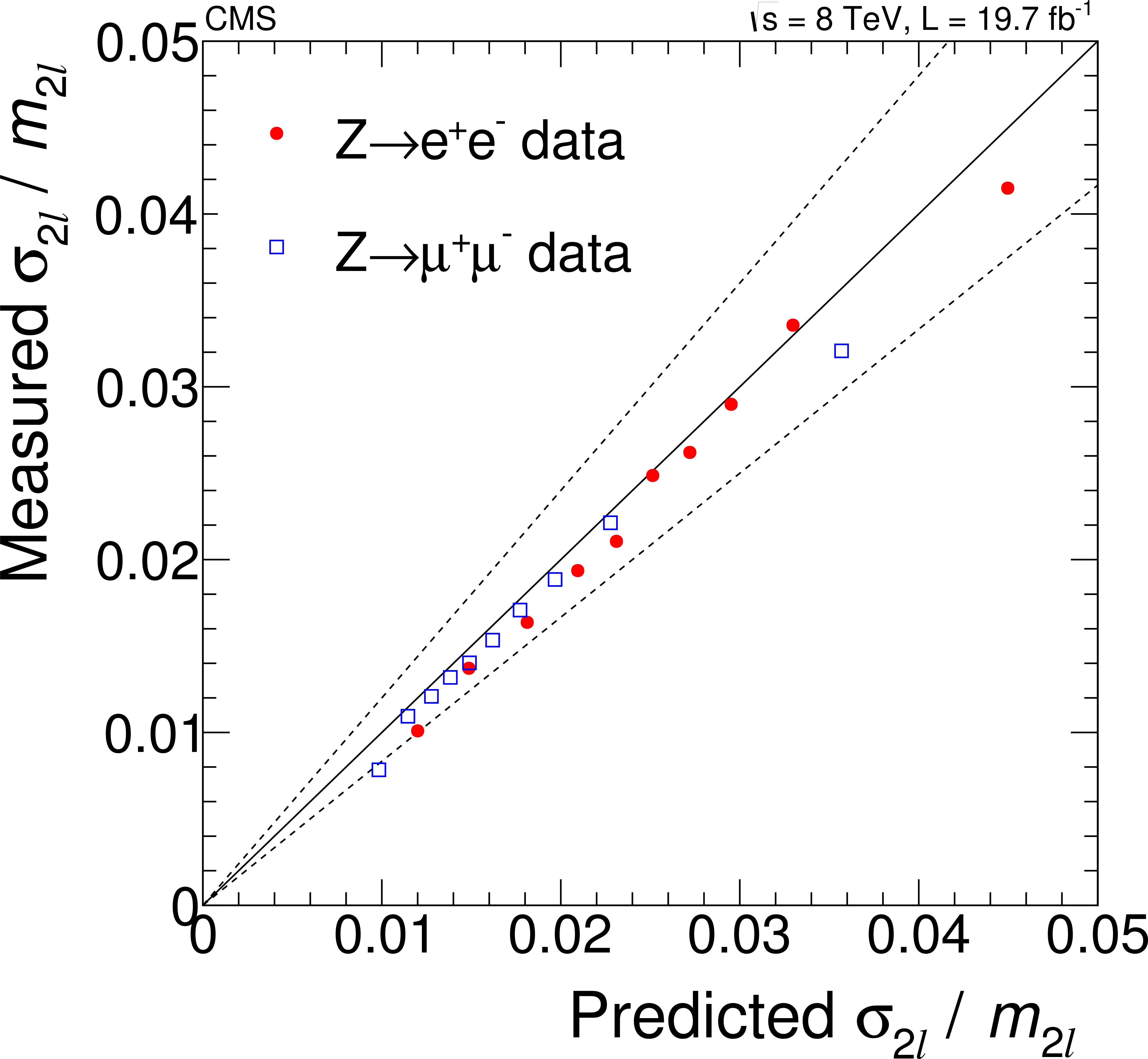
png pdf	Figure 6-a: (a) Measured versus predicted relative mass uncertainties for $ {\mathrm {Z}}\to {\mathrm {e}^+} {\mathrm {e}^-}$ and $ {\mathrm {Z}}\to {{\mu ^+}} {{\mu ^-}}$ events in data. The dashed lines represent the $\pm $20% envelope, used as systematic uncertainty in the resolution. (b) Relative mass uncertainty distribution for data and simulation in the $ {\mathrm {Z}}\to 4\ell $ mass region of 80 $ < m_{4\ell } < $ 100 GeV.
png pdf	Figure 6-b: (a) Measured versus predicted relative mass uncertainties for $ {\mathrm {Z}}\to {\mathrm {e}^+} {\mathrm {e}^-}$ and $ {\mathrm {Z}}\to {{\mu ^+}} {{\mu ^-}}$ events in data. The dashed lines represent the $\pm $20% envelope, used as systematic uncertainty in the resolution. (b) Relative mass uncertainty distribution for data and simulation in the $ {\mathrm {Z}}\to 4\ell $ mass region of 80 $ < m_{4\ell } < $ 100 GeV.
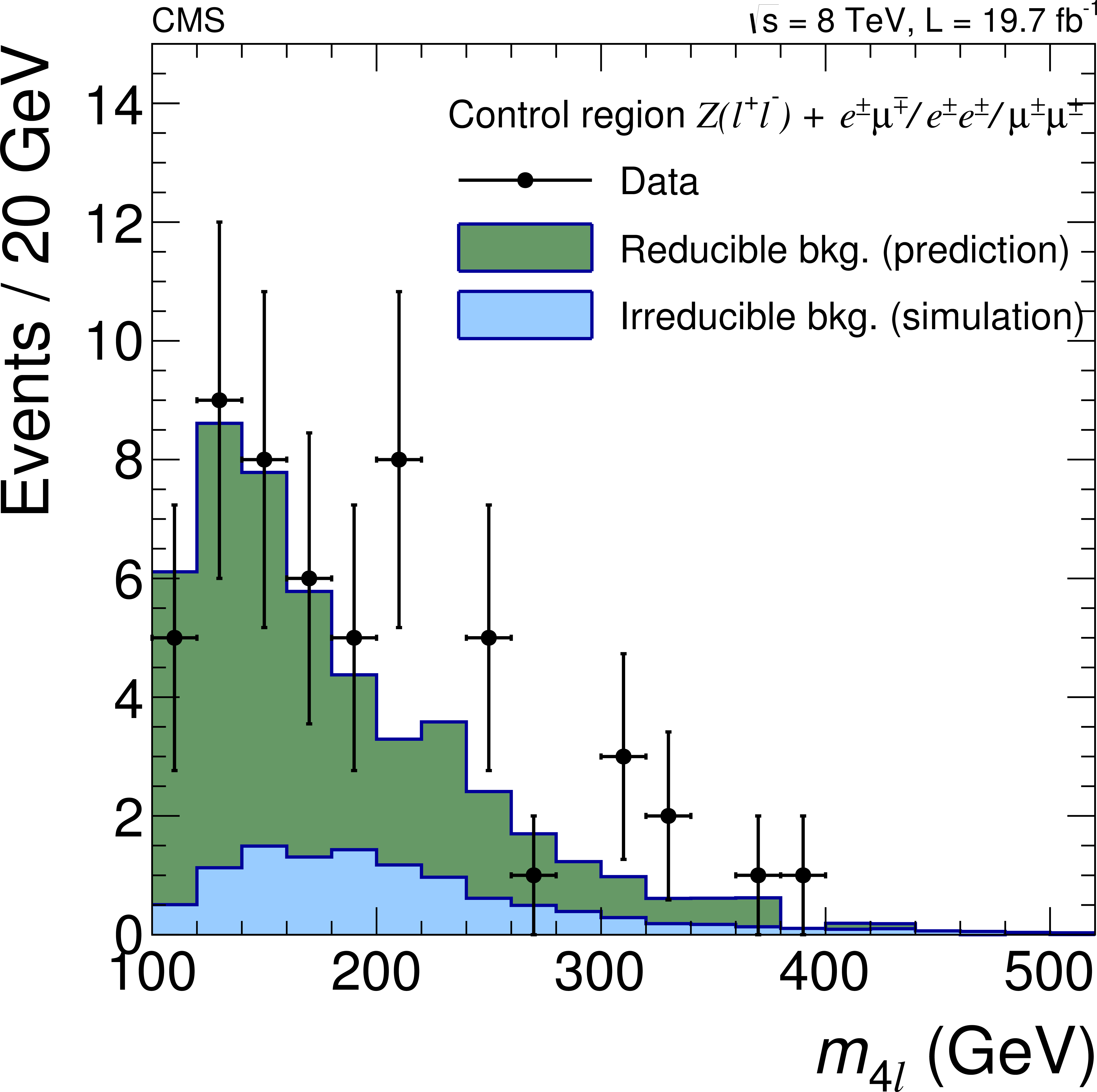
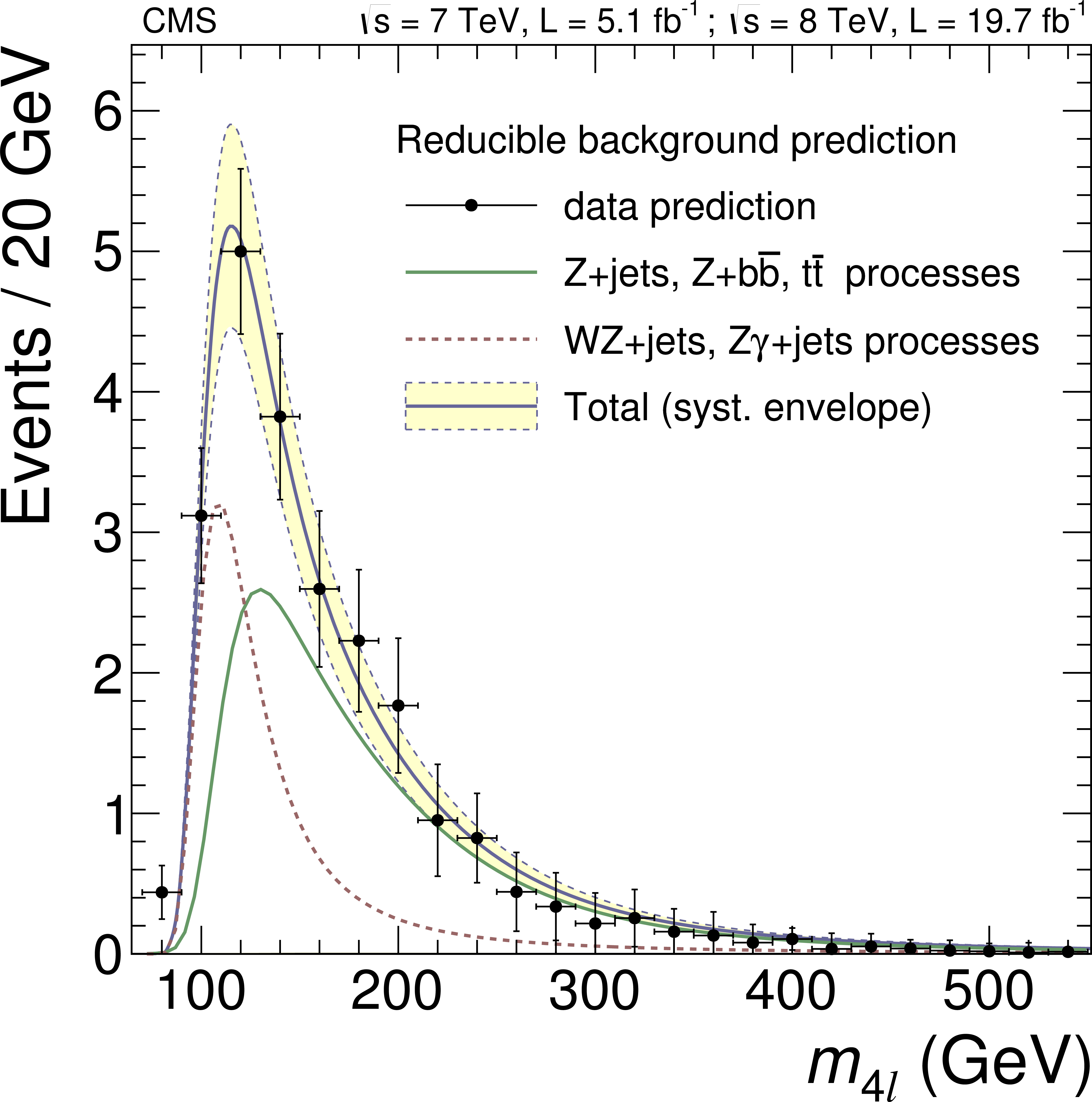
png pdf	Figure 7-a: (a) Validation of the method using the SS control sample. The observed $m_{4\ell }$ distribution (black dots), prediction of the reducible background (dark green area), and expected contributions from $ {\mathrm {Z}} {\mathrm {Z}}$ (light blue area) are shown. (b) Prediction for the reducible background in all three channels together (black dots) fitted using an empirical shape (blue curve) with indicated total uncertainty (yellow band). The contributions from the 2P2F-like (solid green) and 3P1F-like (dashed red) processes are fitted separately.
png pdf	Figure 7-b: (a) Validation of the method using the SS control sample. The observed $m_{4\ell }$ distribution (black dots), prediction of the reducible background (dark green area), and expected contributions from $ {\mathrm {Z}} {\mathrm {Z}}$ (light blue area) are shown. (b) Prediction for the reducible background in all three channels together (black dots) fitted using an empirical shape (blue curve) with indicated total uncertainty (yellow band). The contributions from the 2P2F-like (solid green) and 3P1F-like (dashed red) processes are fitted separately.
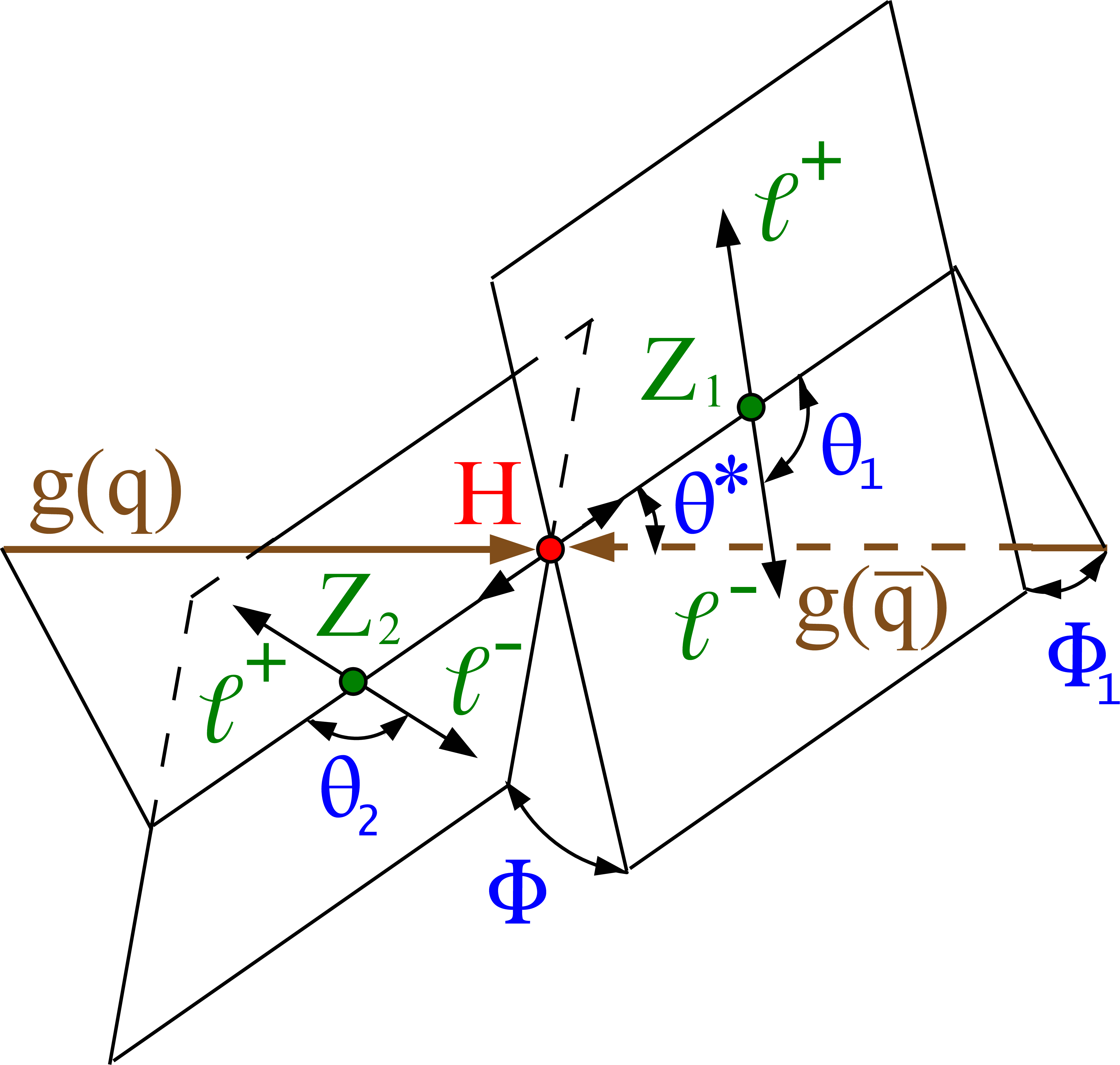
png pdf	Figure 8: Illustration of the production and decay of a particle $ {\mathrm {H}} $, $ {\mathrm {g}} {\mathrm {g}}( {\mathrm {q}} {\overline {\mathrm {q}}})\to {\mathrm {H}} \rightarrow {\mathrm {Z}} {\mathrm {Z}}\rightarrow 4\ell $, with the two production angles $\theta ^*$ and $\Phi _1$ shown in the $ {\mathrm {H}} $ rest frame and three decay angles $\theta _1$, $\theta _2$, and $\Phi $ shown in the $ {\mathrm {Z}}_1$, $ {\mathrm {Z}}_2$, and $ {\mathrm {H}} $ rest frames, respectively.
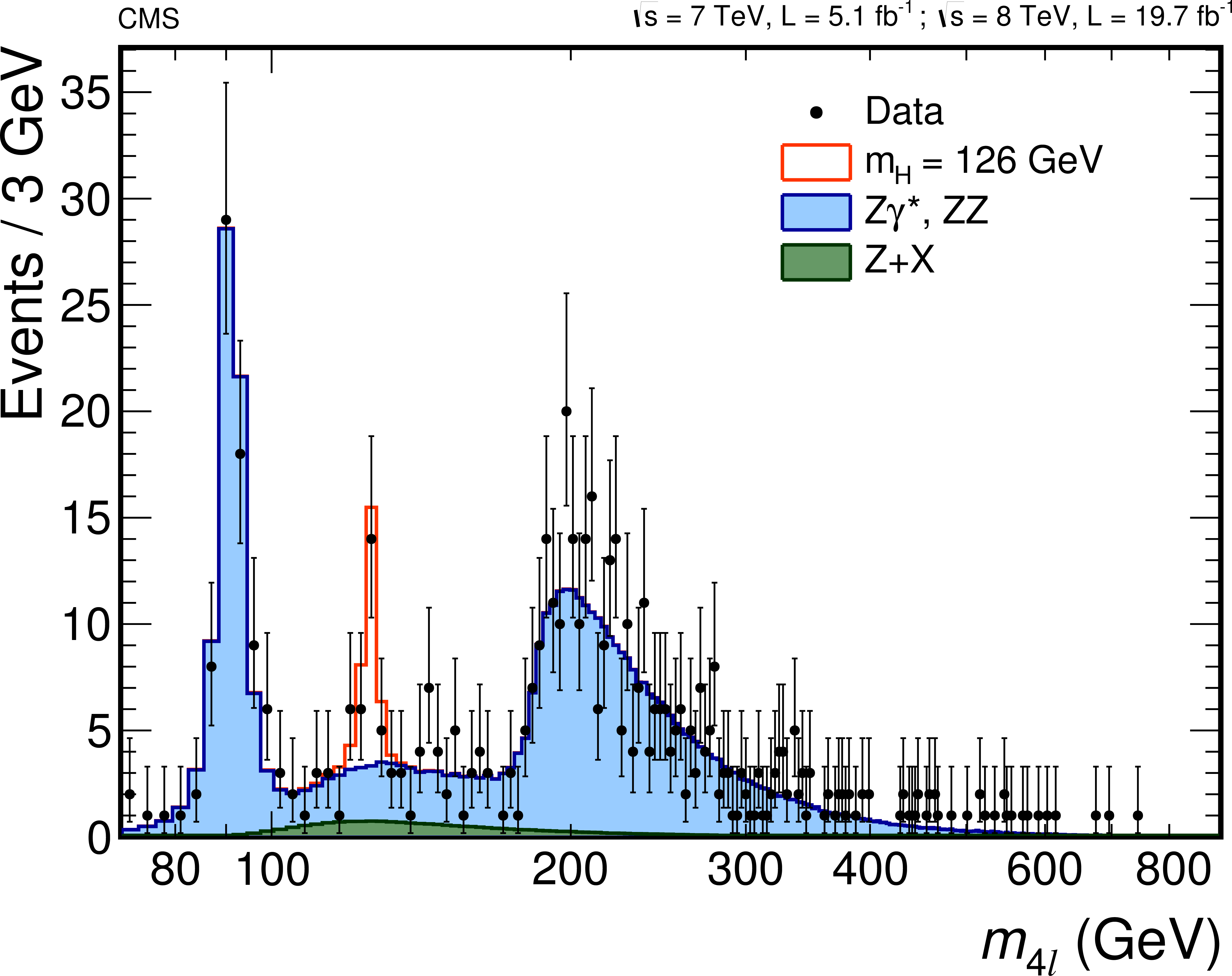
png pdf	Figure 9: Distribution of the four-lepton reconstructed mass in the full mass range $70 < m_{4\ell }< 1000$ GeV for the sum of the $4 {\mathrm {e}}$, $2 {\mathrm {e}}2 {{\mu }}$, and $4 {{\mu }}$ channels. Points with error bars represent the data, shaded histograms represent the backgrounds, and the unshaded histogram represents the signal expectation for a mass hypothesis of $ {m_{ {\mathrm {H}} }}$ = 126 GeV. Signal and the $ {\mathrm {Z}} {\mathrm {Z}}$ background are normalized to the SM expectation; the $ {\mathrm {Z}}+ {\mathrm {X}} $ background to the estimation from data. The expected distributions are presented as stacked histograms. No events are observed with $m_{4\ell } > $ 800 GeV.
png pdf	Figure 10: Distribution of the four-lepton reconstructed mass for the sum of the $4 {\mathrm {e}}$, $2 {\mathrm {e}}2 {{\mu }}$, and $4 {{\mu }}$ channels for the mass region 70 $ < m_{4\ell } < $ 180 GeV. Points with error bars represent the data, shaded histograms represent the backgrounds, and the unshaded histogram represents the signal expectation for a mass hypothesis of $ {m_{ {\mathrm {H}} }} $ = 126 GeV. Signal and the $ {\mathrm {Z}} {\mathrm {Z}}$ background are normalized to the SM expectation, the $ {\mathrm {Z}}+ {\mathrm {X}} $ background to the estimation from data.
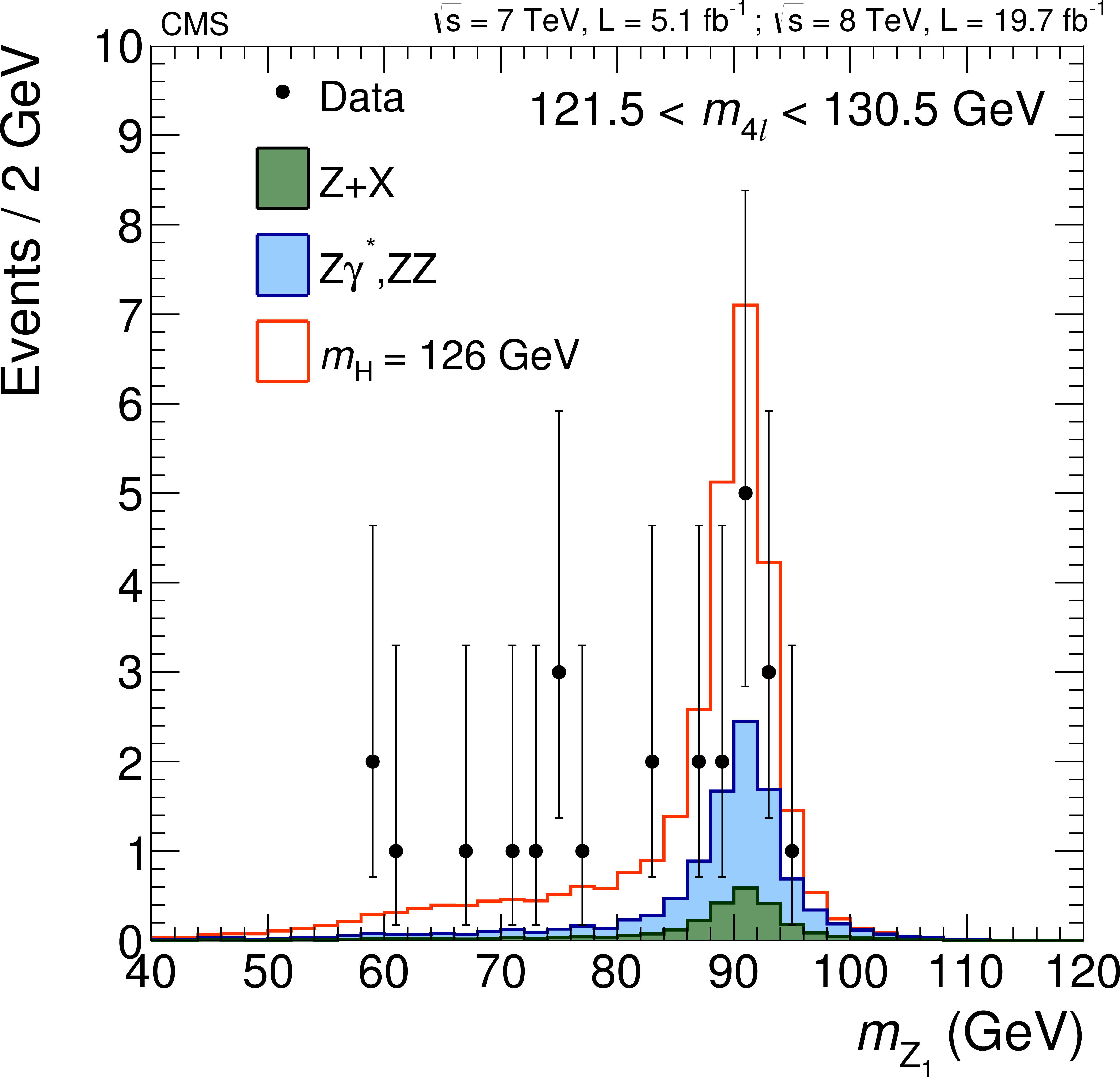
png pdf	Figure 11-a: Distribution of (left) the ${ {\mathrm {Z}}_1}$ and (center) the ${ {\mathrm {Z}}_2}$ reconstructed invariant masses, in the mass region $121.5 < m_{4\ell } < 130.5 GeV $, for the sum of the four-lepton channels. Points represent the data, and shaded histograms represent the background. The signal expectation at $ {m_{ {\mathrm {H}} }} $ = 126 GeV is shown as the unshaded histogram. Signal and background histograms are stacked. (right) Two-dimensional distribution of the two variables in the mass region $106 < m_{4\ell } < 141 GeV $, corresponding to the range used in the signal extraction for $ {m_{ {\mathrm {H}} }} $ = 126 GeV , for the sum of the $4\ell $ channels. The signal expectation at $ {m_{ {\mathrm {H}} }} $ = 126 GeV is shown as the grey scale.
png pdf	Figure 11-b: Distribution of (left) the ${ {\mathrm {Z}}_1}$ and (center) the ${ {\mathrm {Z}}_2}$ reconstructed invariant masses, in the mass region $121.5 < m_{4\ell } < 130.5 GeV $, for the sum of the four-lepton channels. Points represent the data, and shaded histograms represent the background. The signal expectation at $ {m_{ {\mathrm {H}} }} $ = 126 GeV is shown as the unshaded histogram. Signal and background histograms are stacked. (right) Two-dimensional distribution of the two variables in the mass region $106 < m_{4\ell } < 141 GeV $, corresponding to the range used in the signal extraction for $ {m_{ {\mathrm {H}} }} $ = 126 GeV , for the sum of the $4\ell $ channels. The signal expectation at $ {m_{ {\mathrm {H}} }} $ = 126 GeV is shown as the grey scale.
png pdf	Figure 11-c: Distribution of (left) the ${ {\mathrm {Z}}_1}$ and (center) the ${ {\mathrm {Z}}_2}$ reconstructed invariant masses, in the mass region $121.5 < m_{4\ell } < 130.5 GeV $, for the sum of the four-lepton channels. Points represent the data, and shaded histograms represent the background. The signal expectation at $ {m_{ {\mathrm {H}} }} $ = 126 GeV is shown as the unshaded histogram. Signal and background histograms are stacked. (right) Two-dimensional distribution of the two variables in the mass region $106 < m_{4\ell } < 141 GeV $, corresponding to the range used in the signal extraction for $ {m_{ {\mathrm {H}} }} $ = 126 GeV , for the sum of the $4\ell $ channels. The signal expectation at $ {m_{ {\mathrm {H}} }} $ = 126 GeV is shown as the grey scale.
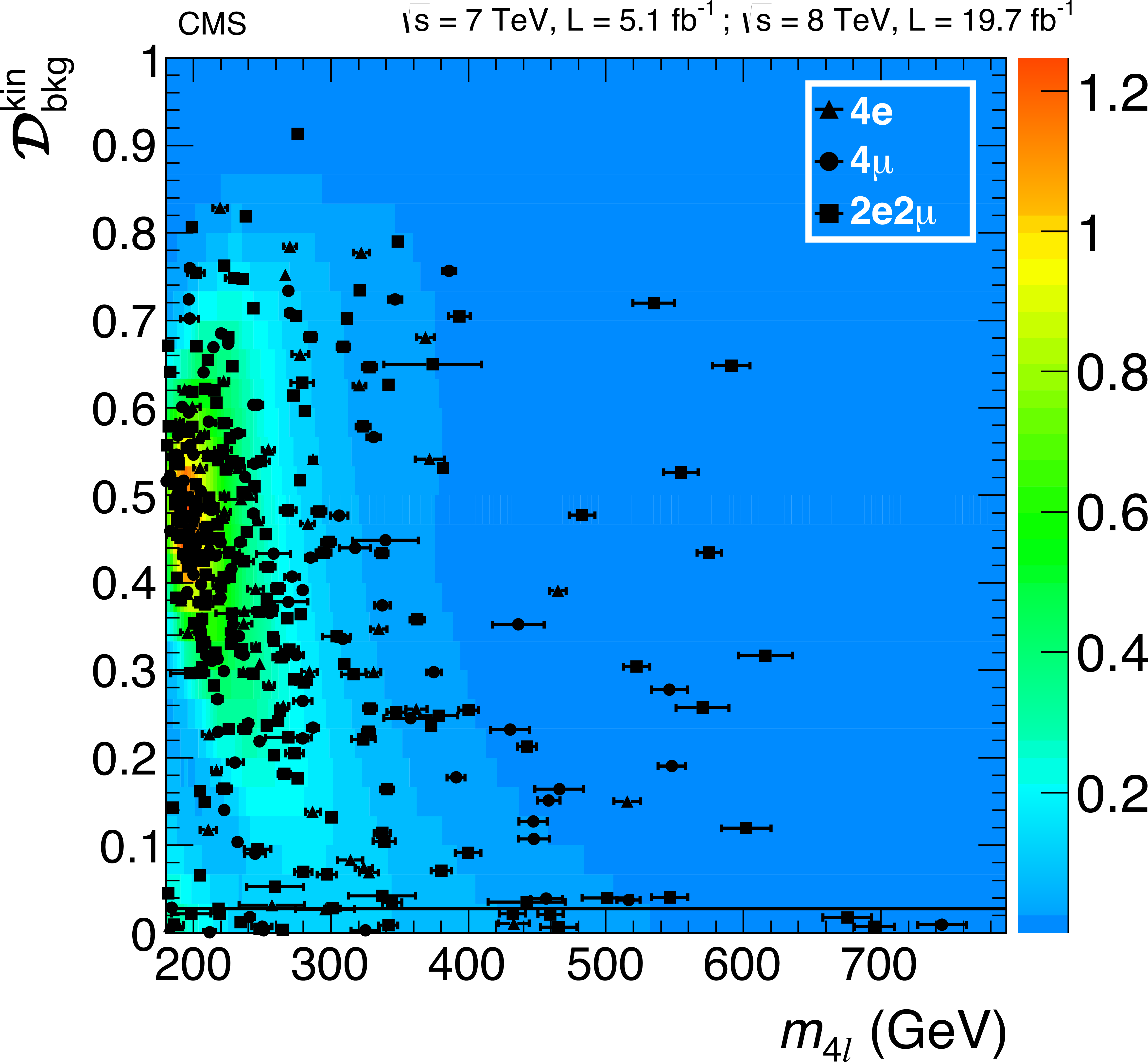
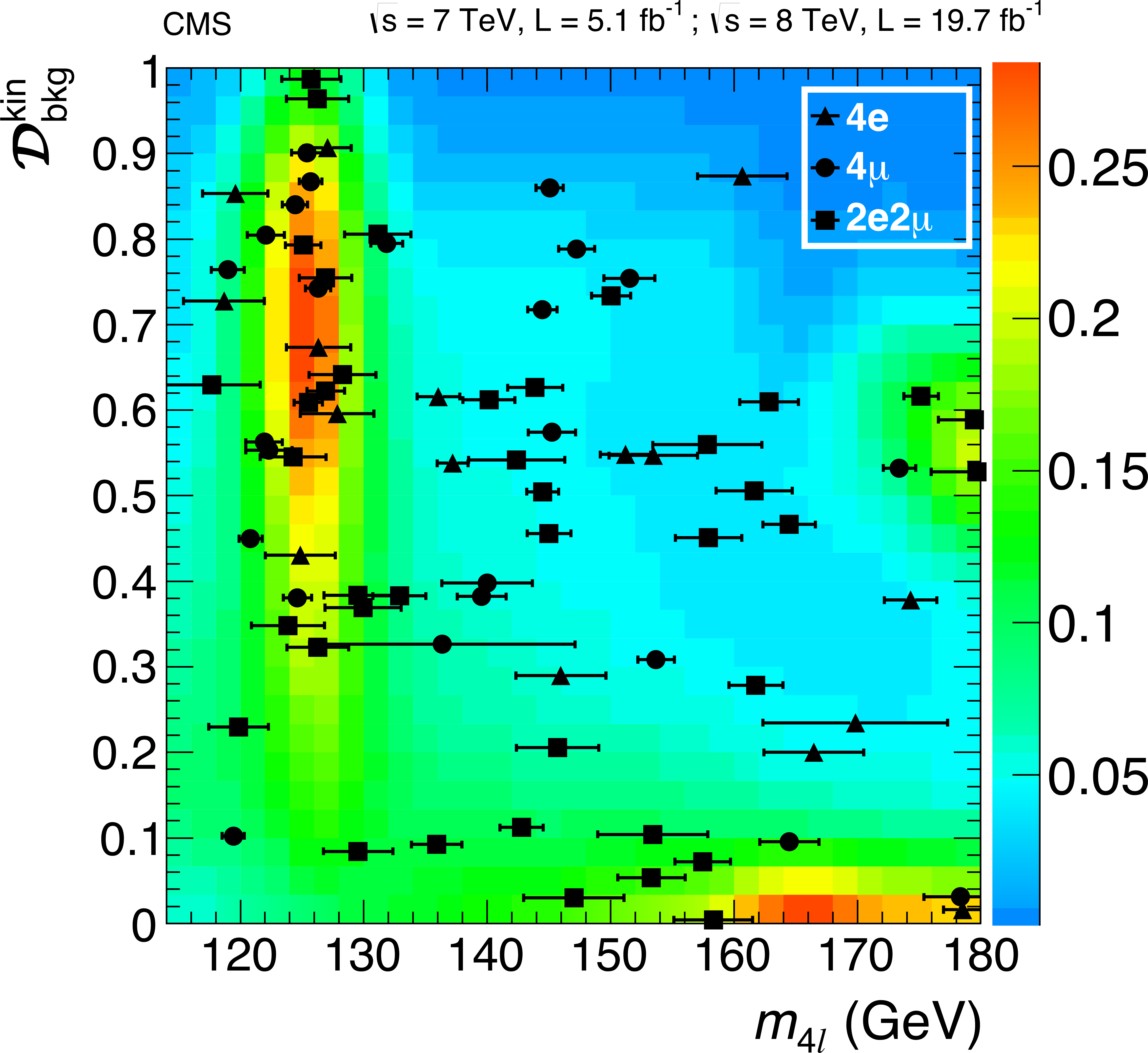
png pdf	Figure 12-a: Distribution of the kinematic discriminant $ {\mathcal {D}^\text {kin}_\text {bkg}} $ versus the four-lepton reconstructed mass $m_{4\ell }$ in the (a) low-mass and (b) high-mass regions. The color scale represents the expected relative density in linear scale (in arbitrary units) of background events. The points show the data and the measured per-event invariant mass uncertainties as horizontal bars. One $2 {\mathrm {e}}2 {{\mu }}$ event with $m_{4\ell }\approx $ 220 GeV and small $ {\mathcal {D}^\text {kin}_\text {bkg}} $ has a huge mass uncertainty, and it is displayed as the horizontal line. No events are observed for $m_{4\ell }>800$ GeV
png pdf	Figure 12-b: Distribution of the kinematic discriminant $ {\mathcal {D}^\text {kin}_\text {bkg}} $ versus the four-lepton reconstructed mass $m_{4\ell }$ in the (a) low-mass and (b) high-mass regions. The color scale represents the expected relative density in linear scale (in arbitrary units) of background events. The points show the data and the measured per-event invariant mass uncertainties as horizontal bars. One $2 {\mathrm {e}}2 {{\mu }}$ event with $m_{4\ell }\approx $ 220 GeV and small $ {\mathcal {D}^\text {kin}_\text {bkg}} $ has a huge mass uncertainty, and it is displayed as the horizontal line. No events are observed for $m_{4\ell }>800$ GeV
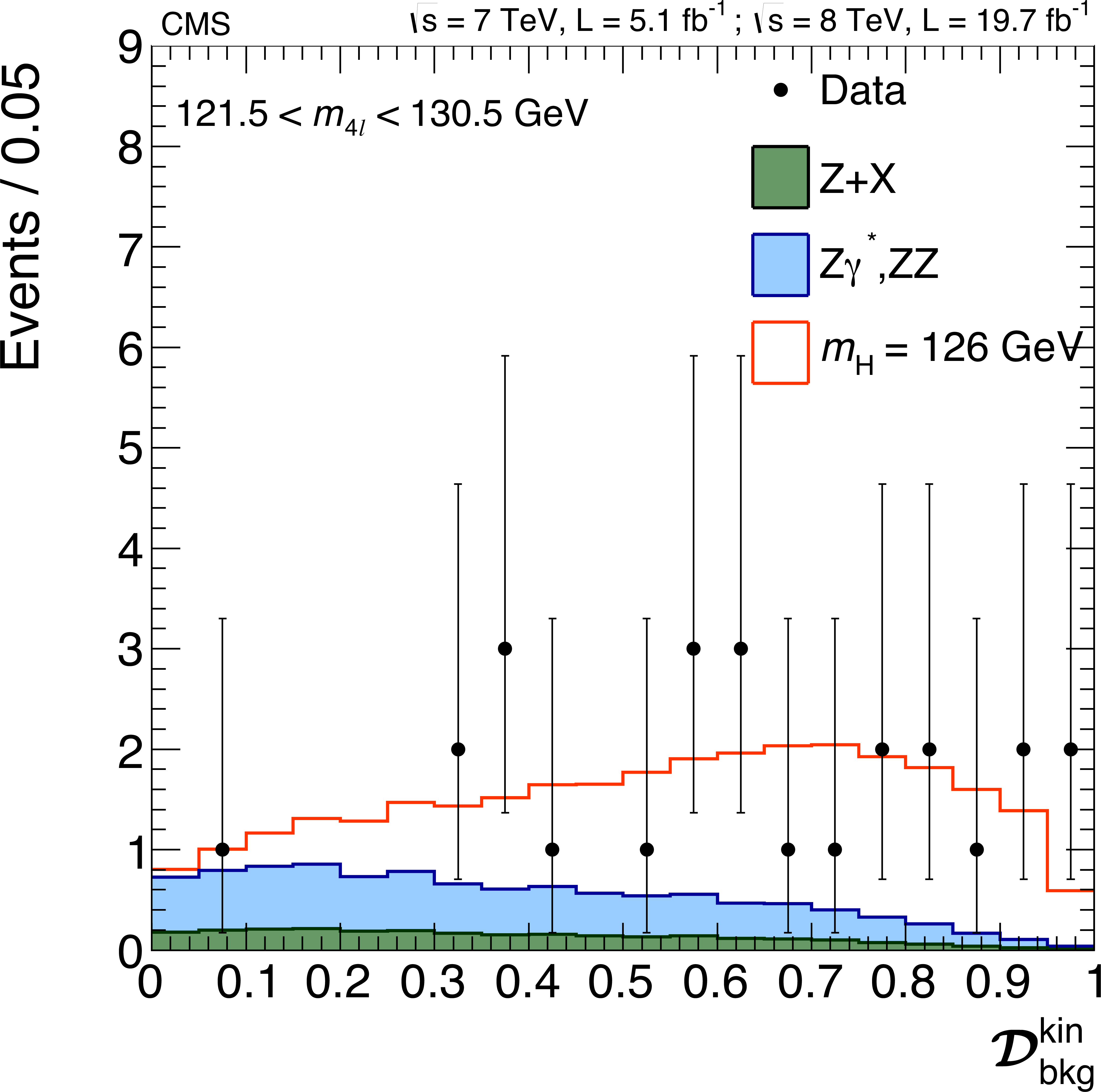
png pdf	Figure 13-a: (a) Distribution of $ {\mathcal {D}^\text {kin}_\text {bkg}} $ versus $m_{4\ell }$ in the low-mass range with colors shown for the expected relative density in linear scale (in arbitrary units) of background plus the Higgs boson signal for $m_{\mathrm{H}} $ = 126 GeV The points show the data, and horizontal bars represent the measured mass uncertainties. (b) Distribution of the kinematic discriminant $ {\mathcal {D}^\text {kin}_\text {bkg}} $ for events in the mass region 121.5 $ < m_{4\ell } < $ 130.5 GeV. Points with error bars represent the data, shaded histograms represent the backgrounds, and the unshaded histogram the signal expectation. Signal and background histograms are stacked.
png pdf	Figure 13-b: (a) Distribution of $ {\mathcal {D}^\text {kin}_\text {bkg}} $ versus $m_{4\ell }$ in the low-mass range with colors shown for the expected relative density in linear scale (in arbitrary units) of background plus the Higgs boson signal for $m_{\mathrm{H}} $ = 126 GeV The points show the data, and horizontal bars represent the measured mass uncertainties. (b) Distribution of the kinematic discriminant $ {\mathcal {D}^\text {kin}_\text {bkg}} $ for events in the mass region 121.5 $ < m_{4\ell } < $ 130.5 GeV. Points with error bars represent the data, shaded histograms represent the backgrounds, and the unshaded histogram the signal expectation. Signal and background histograms are stacked.
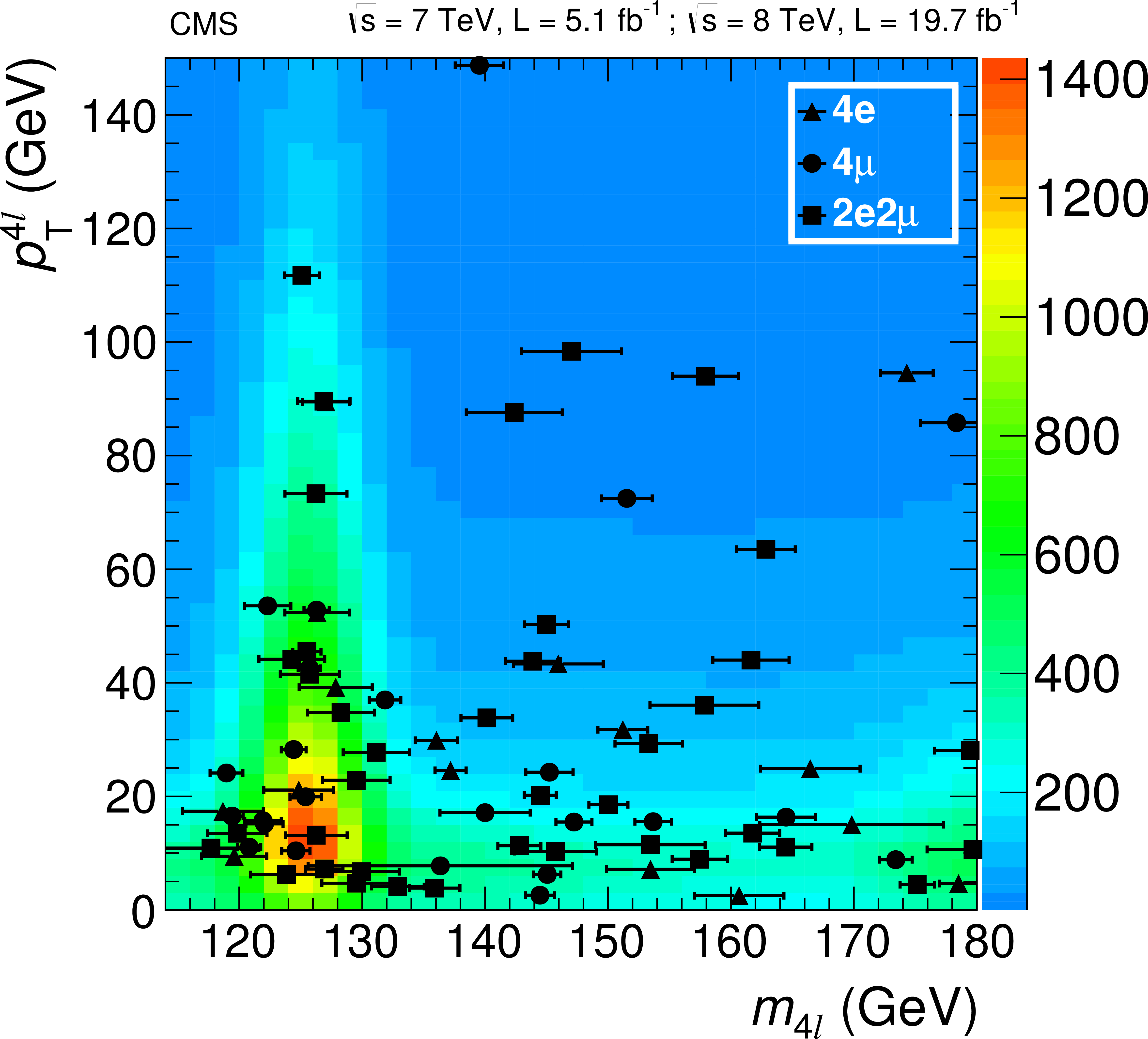
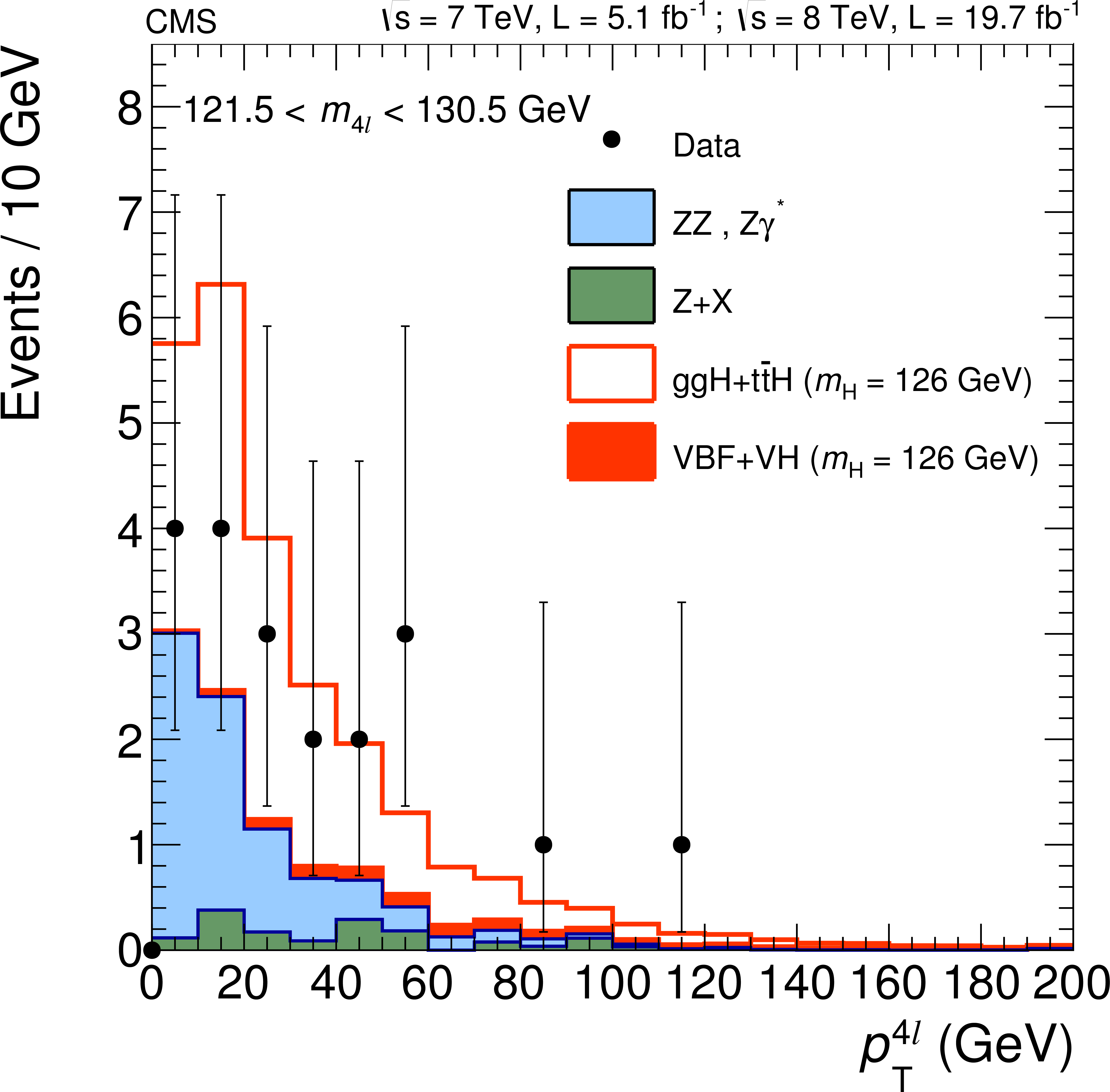
png pdf	Figure 14-a: (a) Distribution of ${ {p_{\mathrm {T}}} ^{4\ell }} $ versus $m_{4\ell }$ in the low-mass-range 0/1-jet category with colors shown for the expected relative density in linear scale (in arbitrary units) of background plus the Higgs boson signal for $m_{\mathrm{H}}$ = 126 GeV No events are observed for $ {p_{\mathrm {T}}} >150$ GeV The points show the data, and horizontal bars represent the measured mass uncertainties. (right) Distribution of ${ {p_{\mathrm {T}}} ^{4\ell }} $ in the 0/1-jet category for events in the mass region $121.5 < m_{4\ell } < 130.5$ GeV Points with error bars represent the data, shaded histograms represent the backgrounds, and the red histograms represent the signal expectation, broken down by production mechanism. Signal and background histograms are stacked.
png pdf	Figure 14-b: (a) Distribution of ${ {p_{\mathrm {T}}} ^{4\ell }} $ versus $m_{4\ell }$ in the low-mass-range 0/1-jet category with colors shown for the expected relative density in linear scale (in arbitrary units) of background plus the Higgs boson signal for $m_{\mathrm{H}}$ = 126 GeV No events are observed for $ {p_{\mathrm {T}}} >150$ GeV The points show the data, and horizontal bars represent the measured mass uncertainties. (right) Distribution of ${ {p_{\mathrm {T}}} ^{4\ell }} $ in the 0/1-jet category for events in the mass region $121.5 < m_{4\ell } < 130.5$ GeV Points with error bars represent the data, shaded histograms represent the backgrounds, and the red histograms represent the signal expectation, broken down by production mechanism. Signal and background histograms are stacked.
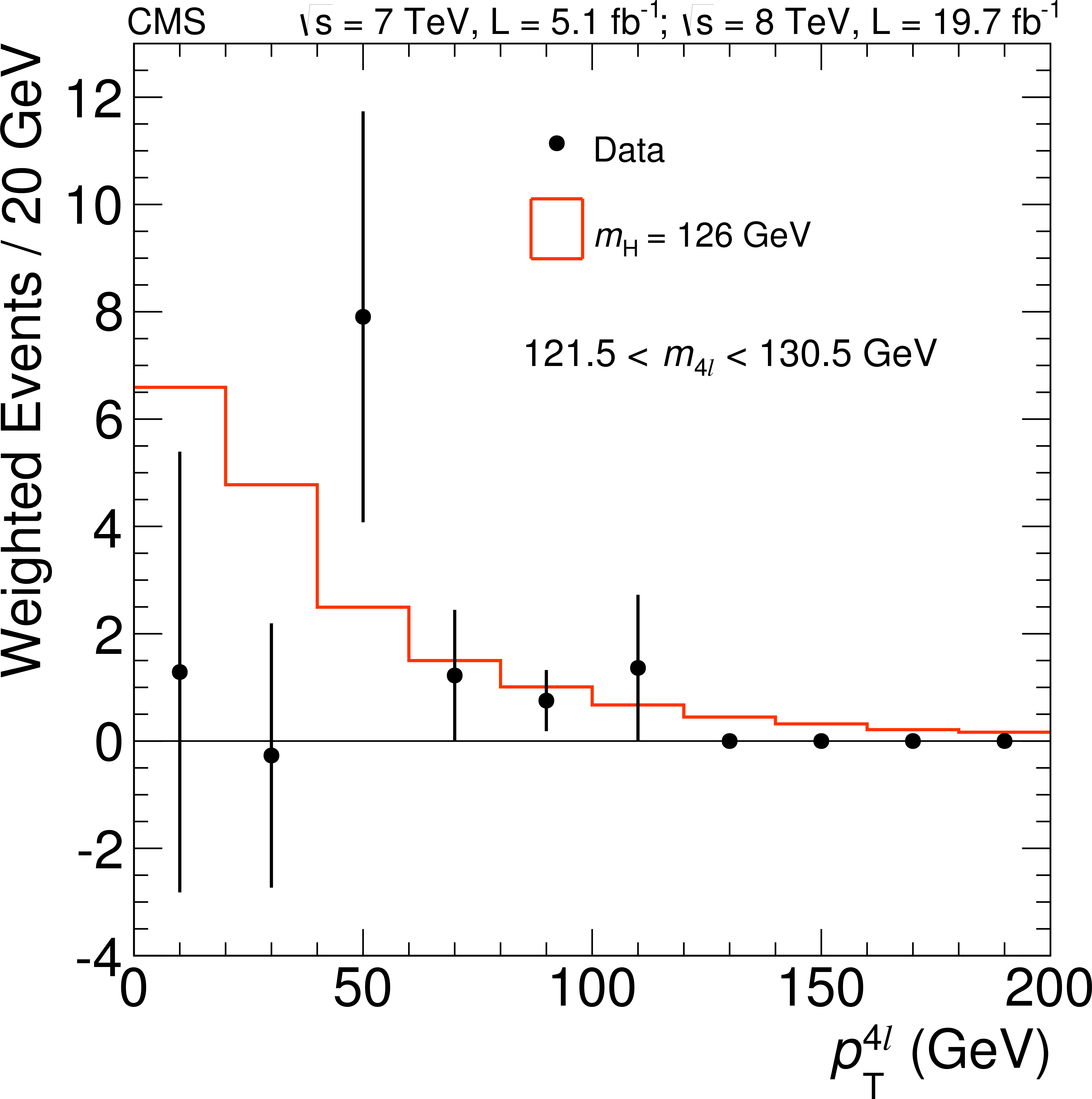
png pdf	Figure 15: ${}_s\mathcal {P}lot$ signal-weighted distribution of the four-lepton system ${ {p_{\mathrm {T}}} ^{4\ell }} $ for all the selected events in the mass region 121.5 $ < m_{4\ell } < $ 130.5 GeV. The red solid line represents the expectation from a SM Higgs boson.
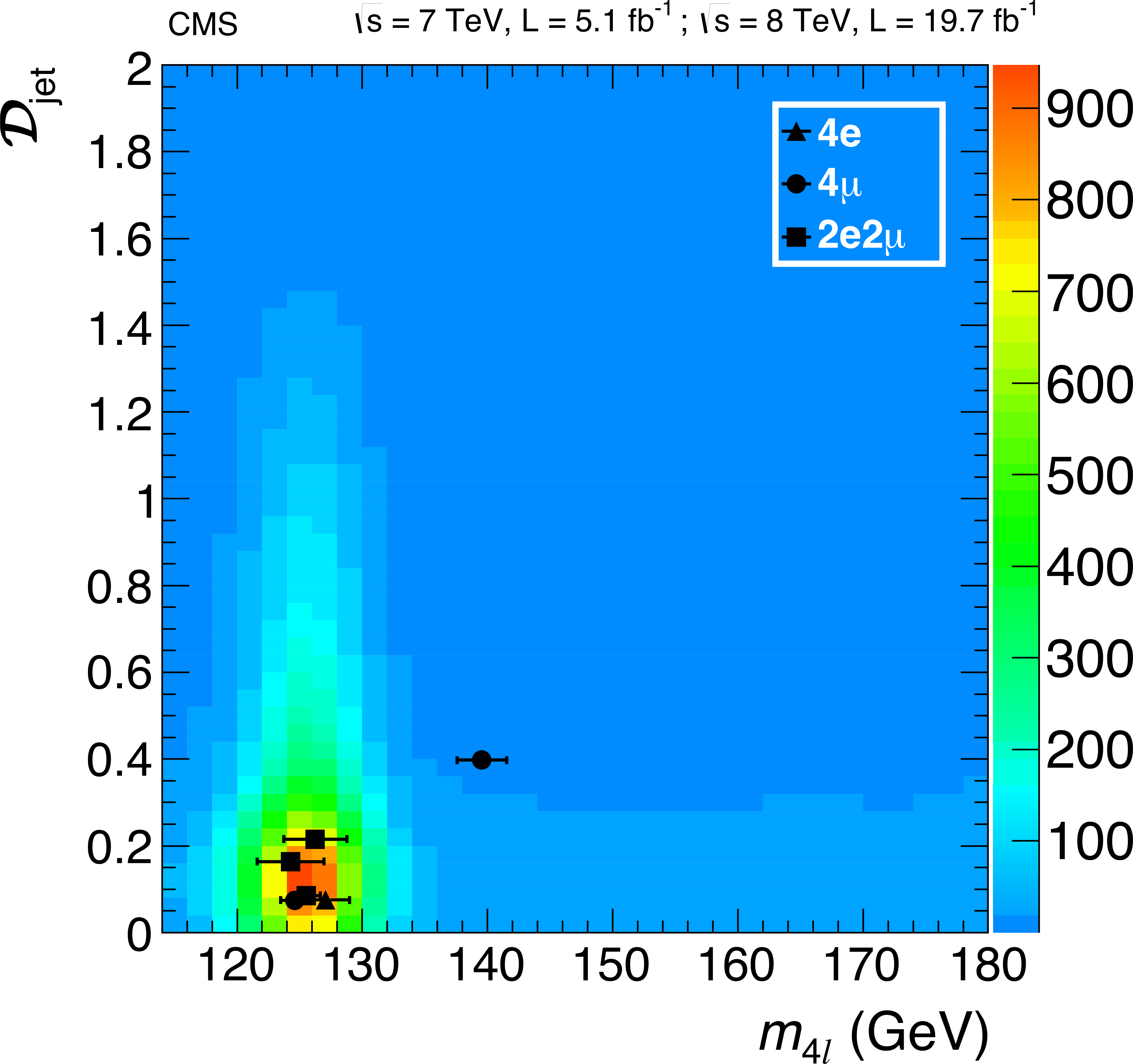
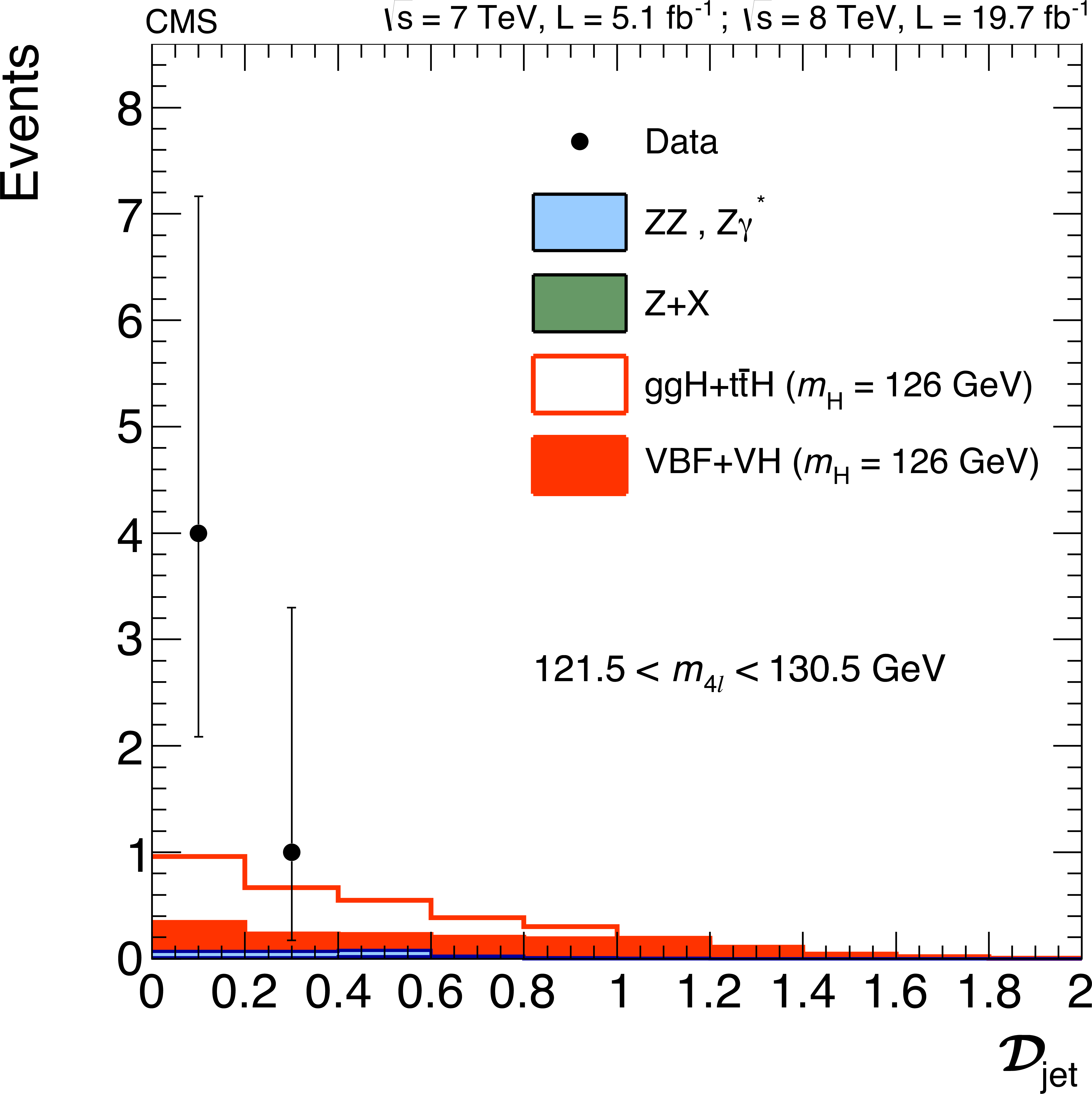
png pdf	Figure 16-a: (a) Distribution of $\mathrm {\mathcal {D}_\text {jet}} $ versus $m_{4\ell }$ in the low-mass-range dijet category with colors shown for the expected relative density in linear scale (in arbitrary units) of background plus the Higgs boson signal for $m_{\mathrm{H}}$ = 126 GeV. The points show the data and horizontal bars represent the measured mass uncertainties. (b) Distribution of $\mathrm {\mathcal {D}_\text {jet}} $ in the dijet category for events in the mass region 121.5 $< m_{4\ell } < $ 130.5 GeV. Points with error bars represent the data, shaded histograms represent the backgrounds, and the red histograms represent the signal expectation, broken down by production mechanism. Signal and background histograms are stacked.
png pdf	Figure 16-b: (a) Distribution of $\mathrm {\mathcal {D}_\text {jet}} $ versus $m_{4\ell }$ in the low-mass-range dijet category with colors shown for the expected relative density in linear scale (in arbitrary units) of background plus the Higgs boson signal for $m_{\mathrm{H}}$ = 126 GeV. The points show the data and horizontal bars represent the measured mass uncertainties. (b) Distribution of $\mathrm {\mathcal {D}_\text {jet}} $ in the dijet category for events in the mass region 121.5 $< m_{4\ell } < $ 130.5 GeV. Points with error bars represent the data, shaded histograms represent the backgrounds, and the red histograms represent the signal expectation, broken down by production mechanism. Signal and background histograms are stacked.
png pdf	Figure 17-a: The $ {\mathrm {H}} \rightarrow {\mathrm {Z}} {\mathrm {Z}}\rightarrow 4\ell $ invariant mass distribution for $ {m_{ {\mathrm {H}} }} $ = 126 GeV in the (a) $4 {\mathrm {e}}$, (b) $2 {\mathrm {e}}2 {{\mu }}$, and (c) $4 {{\mu }}$ channels. The distributions are fitted with a double-sided CB function and the fitted values of the CB width $\sigma _{\mathrm {dCB}}$ are indicated. The values of effective resolution, defined as half the smallest width that contains 68.3% of the distribution, are also indicated. The distributions are arbitrarily normalized.
png pdf	Figure 17-b: The $ {\mathrm {H}} \rightarrow {\mathrm {Z}} {\mathrm {Z}}\rightarrow 4\ell $ invariant mass distribution for $ {m_{ {\mathrm {H}} }} $ = 126 GeV in the (a) $4 {\mathrm {e}}$, (b) $2 {\mathrm {e}}2 {{\mu }}$, and (c) $4 {{\mu }}$ channels. The distributions are fitted with a double-sided CB function and the fitted values of the CB width $\sigma _{\mathrm {dCB}}$ are indicated. The values of effective resolution, defined as half the smallest width that contains 68.3% of the distribution, are also indicated. The distributions are arbitrarily normalized.
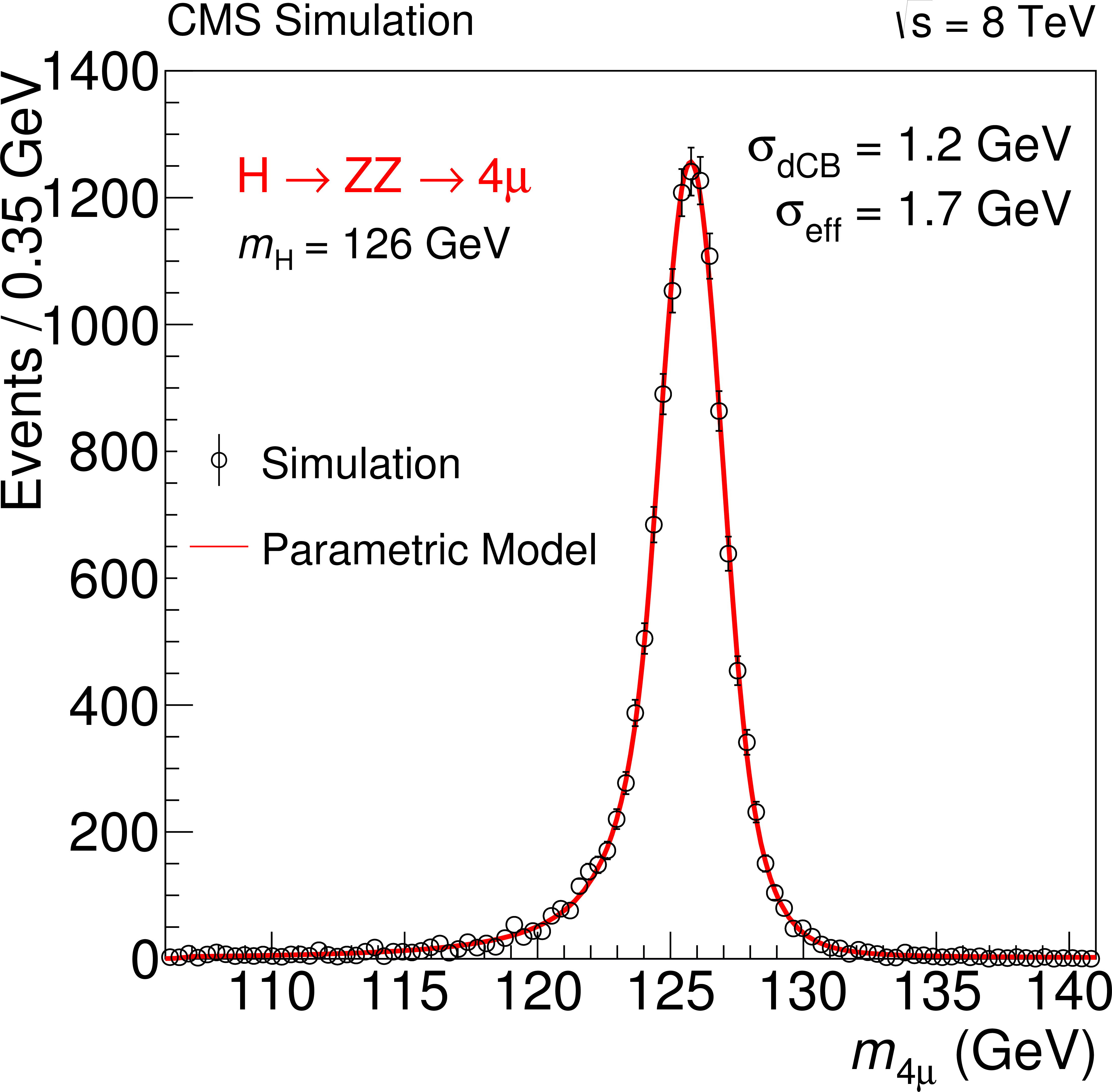
png pdf	Figure 17-c: The $ {\mathrm {H}} \rightarrow {\mathrm {Z}} {\mathrm {Z}}\rightarrow 4\ell $ invariant mass distribution for $ {m_{ {\mathrm {H}} }} $ = 126 GeV in the (a) $4 {\mathrm {e}}$, (b) $2 {\mathrm {e}}2 {{\mu }}$, and (c) $4 {{\mu }}$ channels. The distributions are fitted with a double-sided CB function and the fitted values of the CB width $\sigma _{\mathrm {dCB}}$ are indicated. The values of effective resolution, defined as half the smallest width that contains 68.3% of the distribution, are also indicated. The distributions are arbitrarily normalized.
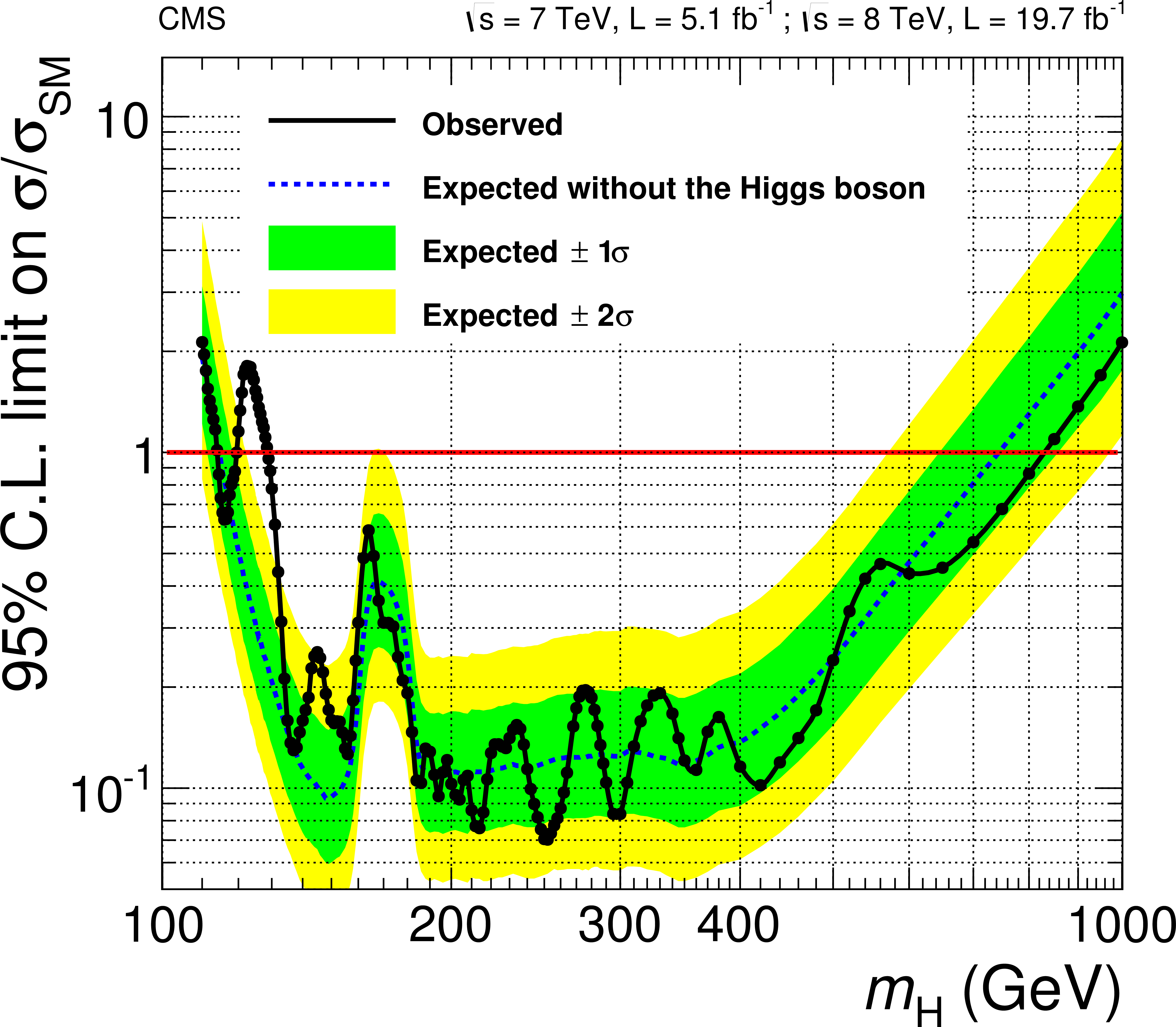
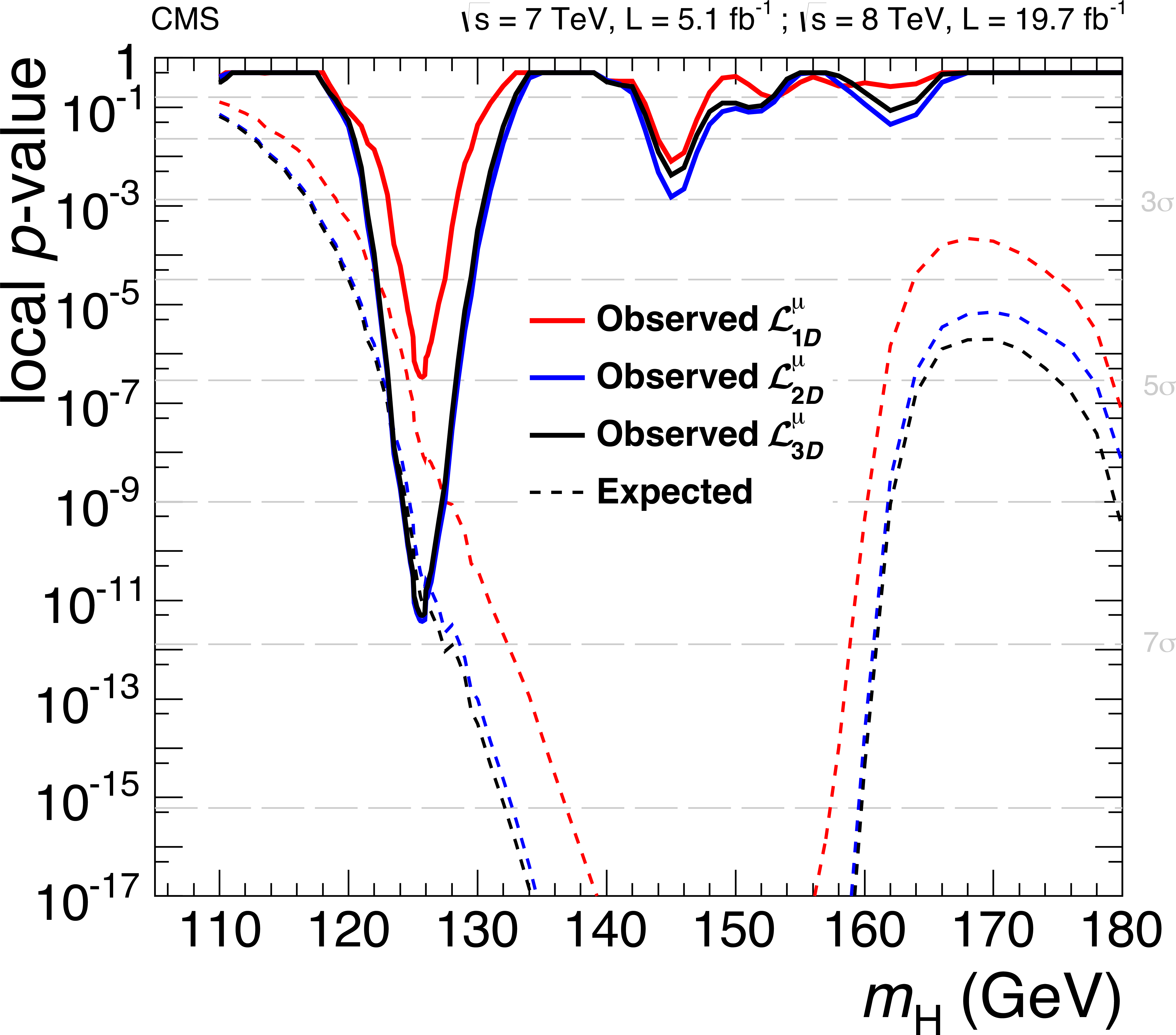
png pdf	Figure 18-a: (a) Observed and expected 95% CL upper limit on the ratio of the production cross section to the SM expectation. The expected 1$\sigma $ and 2$\sigma $ ranges of expectation for the background-only model are also shown with green and yellow bands, respectively. (right) Significance of the local excess with respect to the SM background expectation as a function of the Higgs boson mass in the full mass range 110--1000 GeV Results are shown for the 1D fit ($\mathcal {L}_{1D}^{\mu } $), the 2D fit ($\mathcal {L}_{2D}^{\mu } $), and the reference 3D fit ($\mathcal {L}_{3D}^{\mu } $).
png pdf	Figure 18-b: (a) Observed and expected 95% CL upper limit on the ratio of the production cross section to the SM expectation. The expected 1$\sigma $ and 2$\sigma $ ranges of expectation for the background-only model are also shown with green and yellow bands, respectively. (right) Significance of the local excess with respect to the SM background expectation as a function of the Higgs boson mass in the full mass range 110--1000 GeV Results are shown for the 1D fit ($\mathcal {L}_{1D}^{\mu } $), the 2D fit ($\mathcal {L}_{2D}^{\mu } $), and the reference 3D fit ($\mathcal {L}_{3D}^{\mu } $).
png pdf	Figure 19: Significance of the local excess with respect to the SM background expectation as a function of the Higgs boson mass for the 1D fit ($\mathcal {L}_{1D}^{\mu } $), the 2D fit ($\mathcal {L}_{2D}^{\mu } $), and the reference 3D fit ($\mathcal {L}_{3D}^{\mu } $). Results are shown for the full data sample in the low-mass region only.
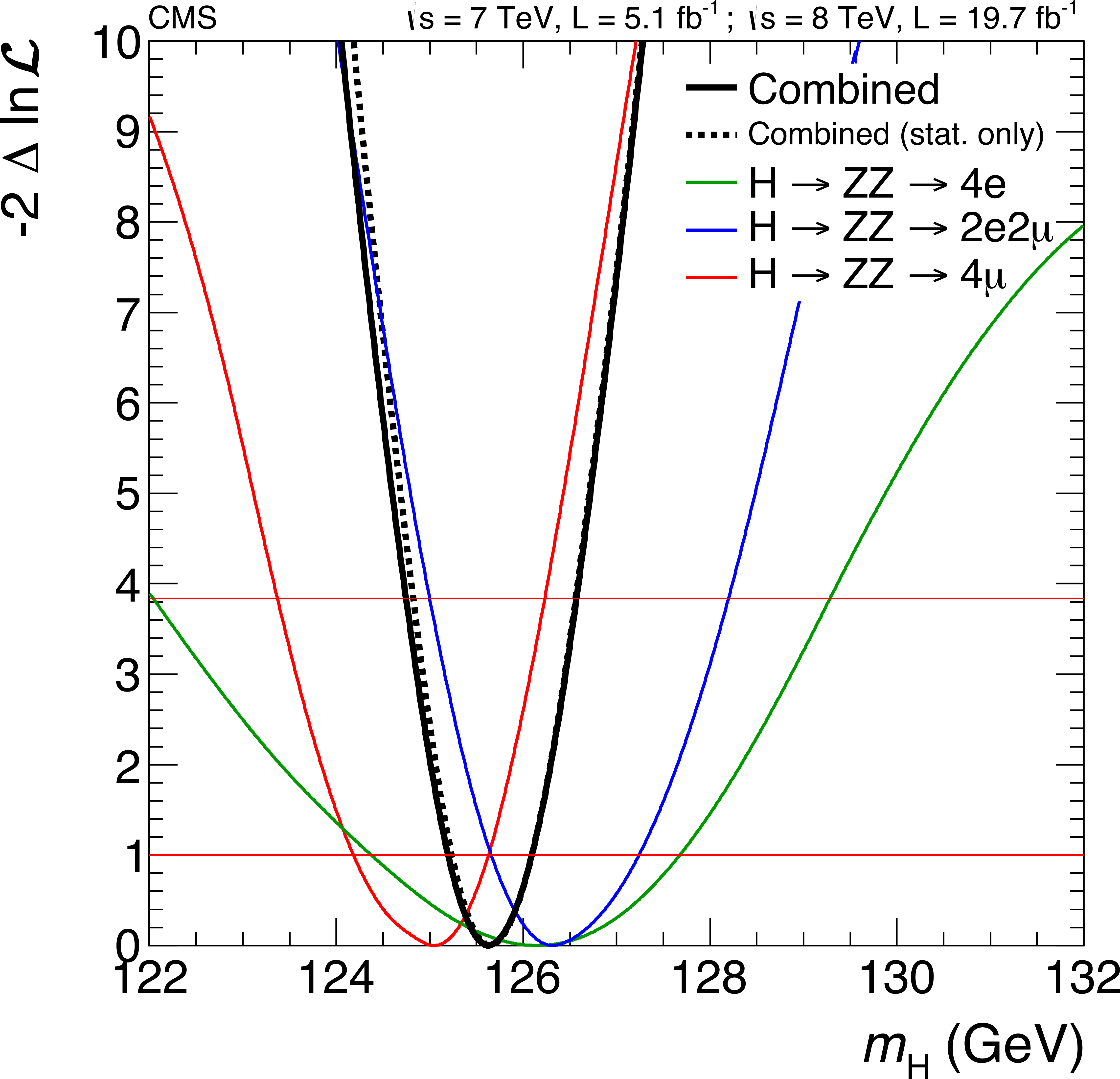
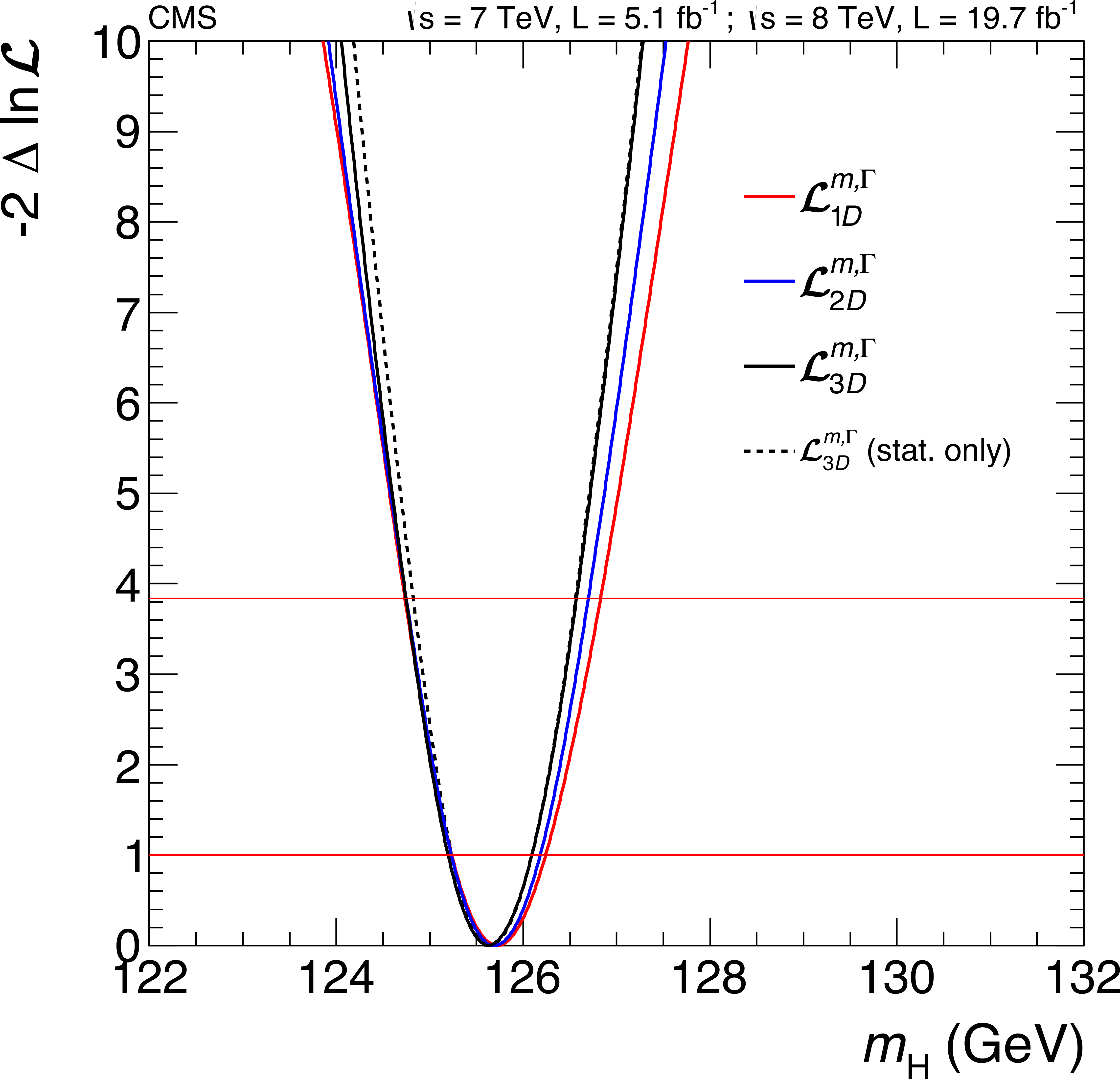
png pdf	Figure 20-a: (a) Scan of the negative log likelihood $-2\Delta \ln{\mathcal {L}}$ versus the SM Higgs boson mass $ {m_{ {\mathrm {H}} }}$, for each of the three channels separately and the combination of the three, where the dashed line represents the scan including only statistical uncertainties when using the 3D model. (right) Scan of $-2\Delta \ln{ \mathcal {L} }$ versus $ {m_{ {\mathrm {H}} }}$ for the combination of the three channels, and using the 1D fit ($\mathcal {L}_{1D}^{m,\Gamma } )$, 2D fit ($\mathcal {L}_{2D}^{m,\Gamma } $), and 3D fit ($\mathcal {L}_{3D}^{m,\Gamma } $). The horizontal lines at $-2\Delta \ln{ \mathcal {L} } = 1$ and 3.84 represent the 68% and 95% CL's, respectively.
png pdf	Figure 20-b: (a) Scan of the negative log likelihood $-2\Delta \ln{\mathcal {L}}$ versus the SM Higgs boson mass $ {m_{ {\mathrm {H}} }}$, for each of the three channels separately and the combination of the three, where the dashed line represents the scan including only statistical uncertainties when using the 3D model. (right) Scan of $-2\Delta \ln{ \mathcal {L} }$ versus $ {m_{ {\mathrm {H}} }}$ for the combination of the three channels, and using the 1D fit ($\mathcal {L}_{1D}^{m,\Gamma } )$, 2D fit ($\mathcal {L}_{2D}^{m,\Gamma } $), and 3D fit ($\mathcal {L}_{3D}^{m,\Gamma } $). The horizontal lines at $-2\Delta \ln{ \mathcal {L} } = 1$ and 3.84 represent the 68% and 95% CL's, respectively.
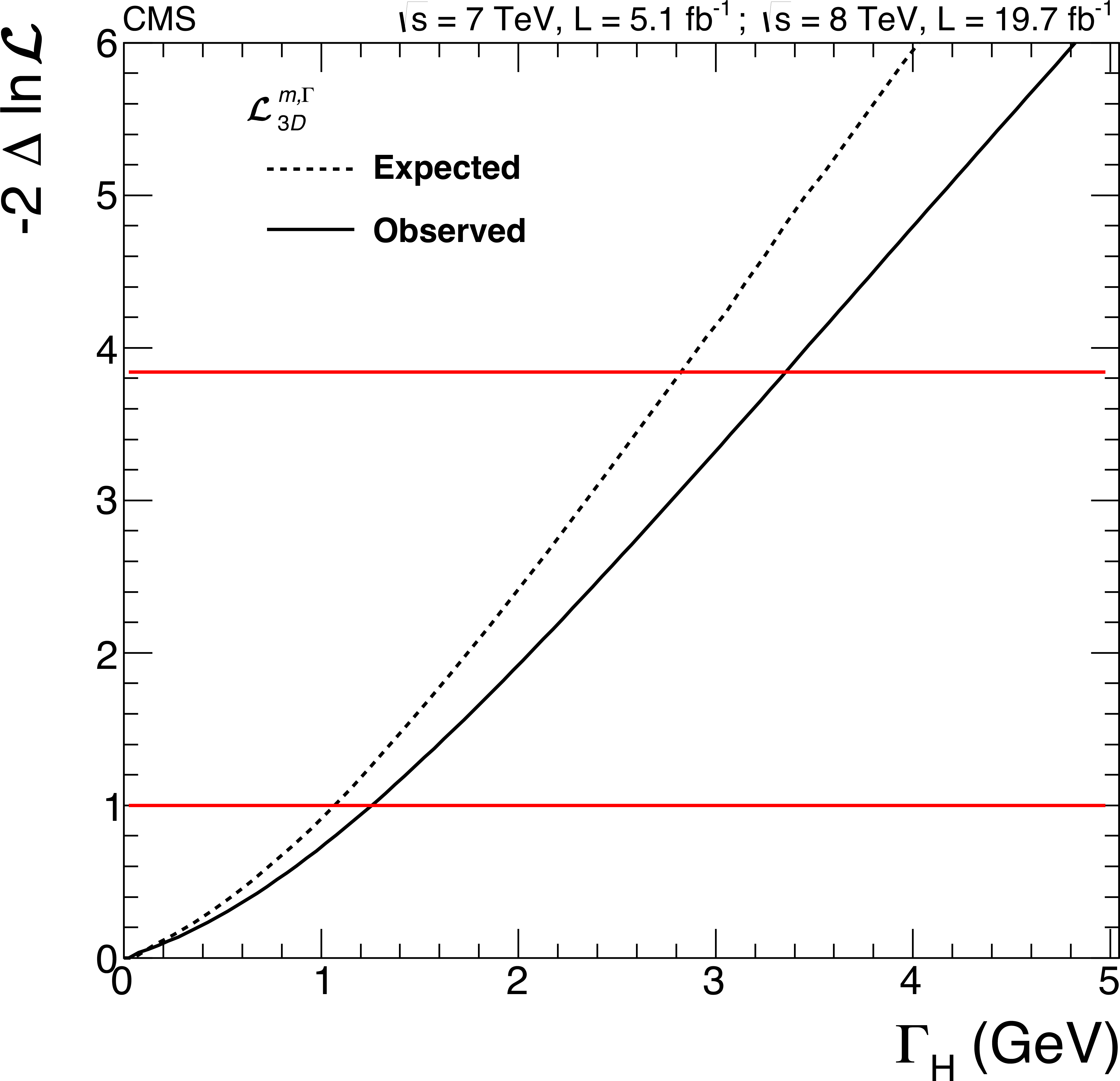
png pdf	Figure 21: Scan of the average expected and observed negative log likelihood $-2\Delta \ln{ \mathcal {L} }$ versus the tested SM Higgs boson width $\Gamma _{ {\mathrm {H}} }$ obtained with the 3D fit ($\mathcal {L}_{3D}^{m,\Gamma } $). The horizontal lines at $-2\Delta \ln{ \mathcal {L} }$ = 1 and 3.84 represent the 68% and 95% CL's, respectively.
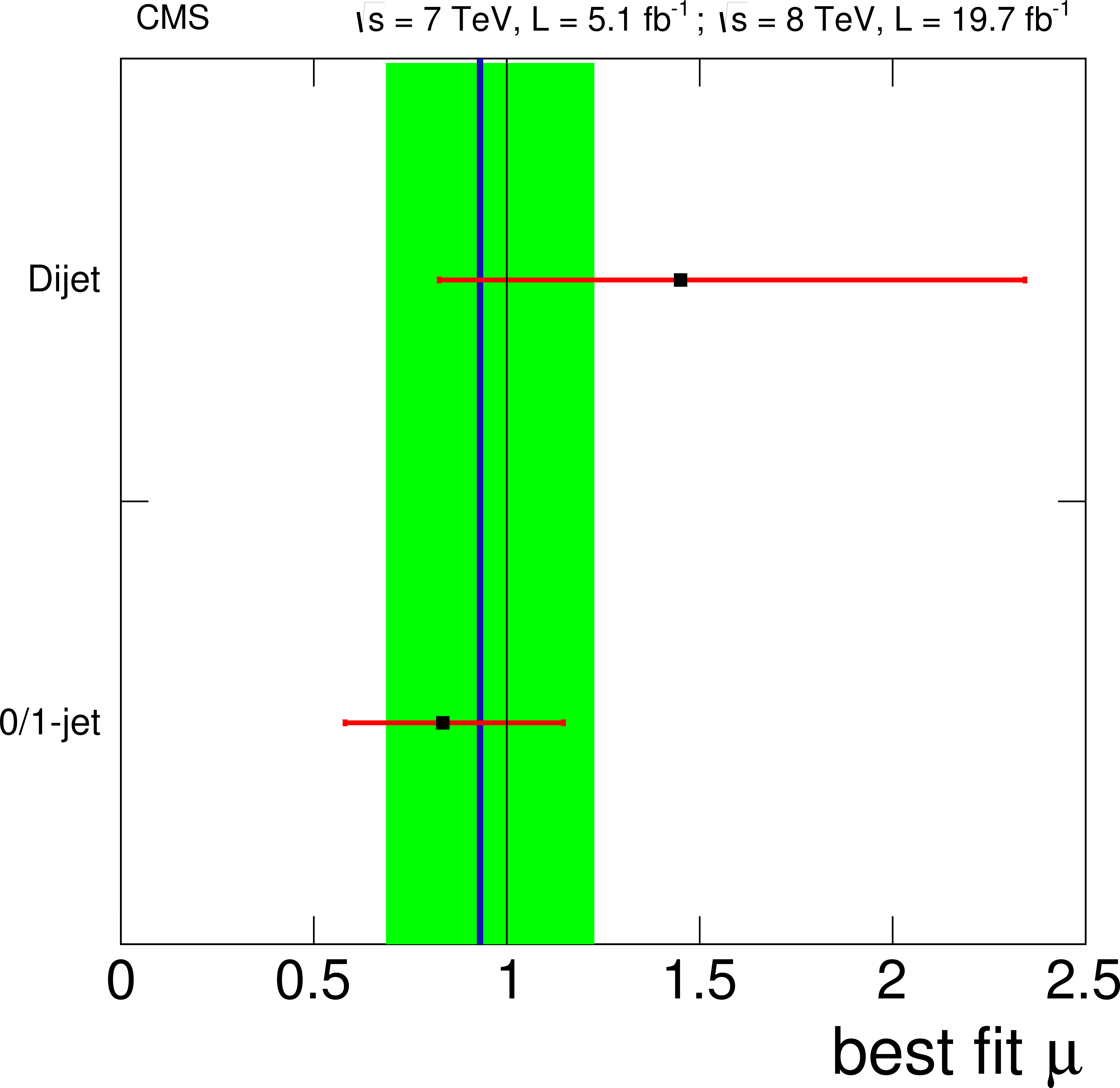
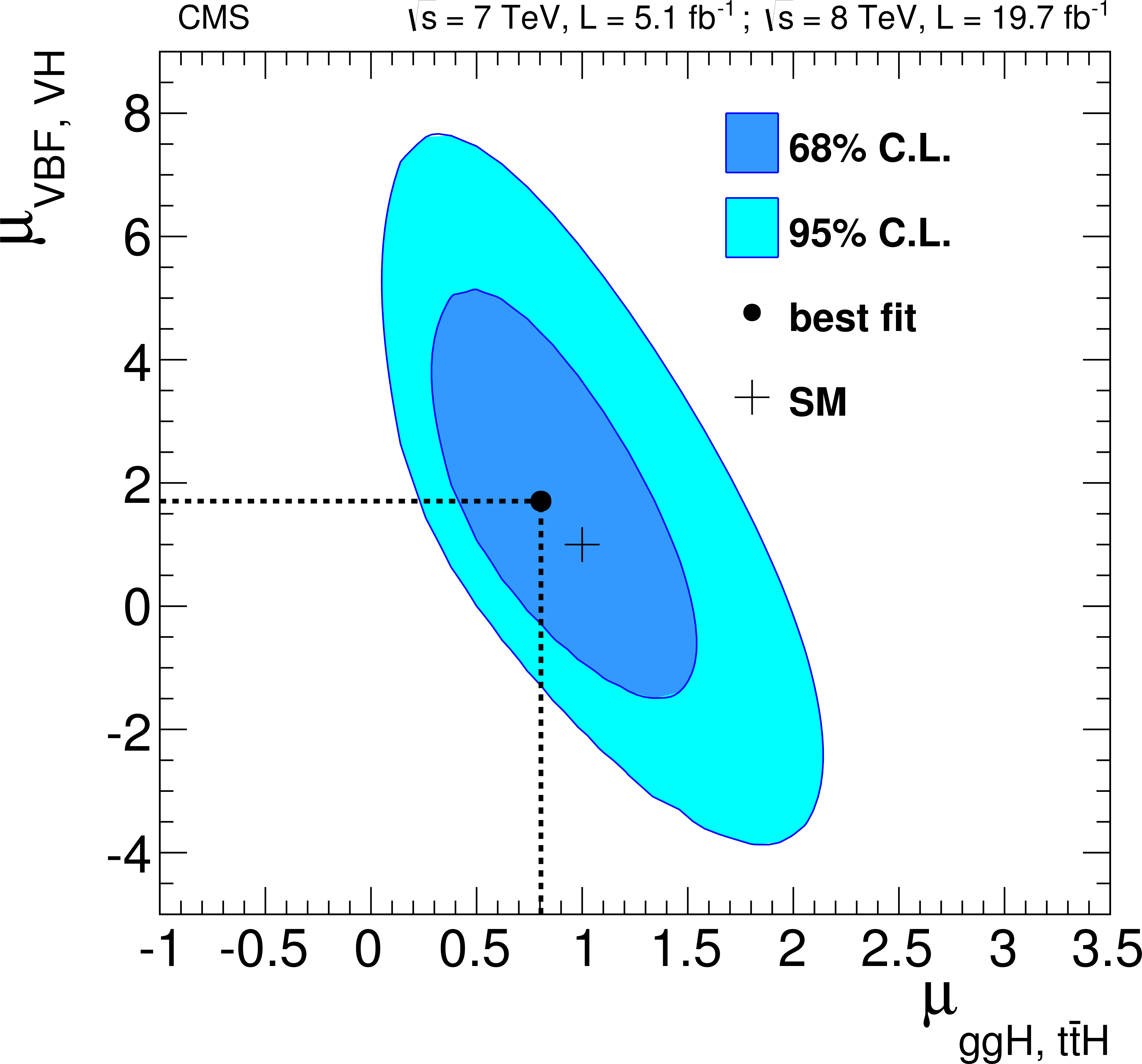
png pdf	Figure 22-a: (a) Values of $ {\mu }$ for the two categories. The vertical line shows the combined $ {\mu }$ together with its associated ${\pm }1\sigma $ uncertainties, shown as a green band. The horizontal bars indicate the ${\pm }1\sigma $ uncertainties in $ {\mu }$ for the different categories. The uncertainties include both statistical and systematic sources of uncertainty. (b) Likelihood contours on the signal-strength modifiers associated with fermions ($ {\mu _{ {\mathrm {g}} {\mathrm {g}} {\mathrm {H}} , \, {\mathrm {t}\overline {\mathrm {t}}} {\mathrm {H}} }} $) and vector bosons ($ {\mu _{\mathrm {VBF},\, \mathrm {V {\mathrm {H}} }}} $) shown at a 68% and 95% CL.
png pdf	Figure 22-b: (a) Values of $ {\mu }$ for the two categories. The vertical line shows the combined $ {\mu }$ together with its associated ${\pm }1\sigma $ uncertainties, shown as a green band. The horizontal bars indicate the ${\pm }1\sigma $ uncertainties in $ {\mu }$ for the different categories. The uncertainties include both statistical and systematic sources of uncertainty. (b) Likelihood contours on the signal-strength modifiers associated with fermions ($ {\mu _{ {\mathrm {g}} {\mathrm {g}} {\mathrm {H}} , \, {\mathrm {t}\overline {\mathrm {t}}} {\mathrm {H}} }} $) and vector bosons ($ {\mu _{\mathrm {VBF},\, \mathrm {V {\mathrm {H}} }}} $) shown at a 68% and 95% CL.
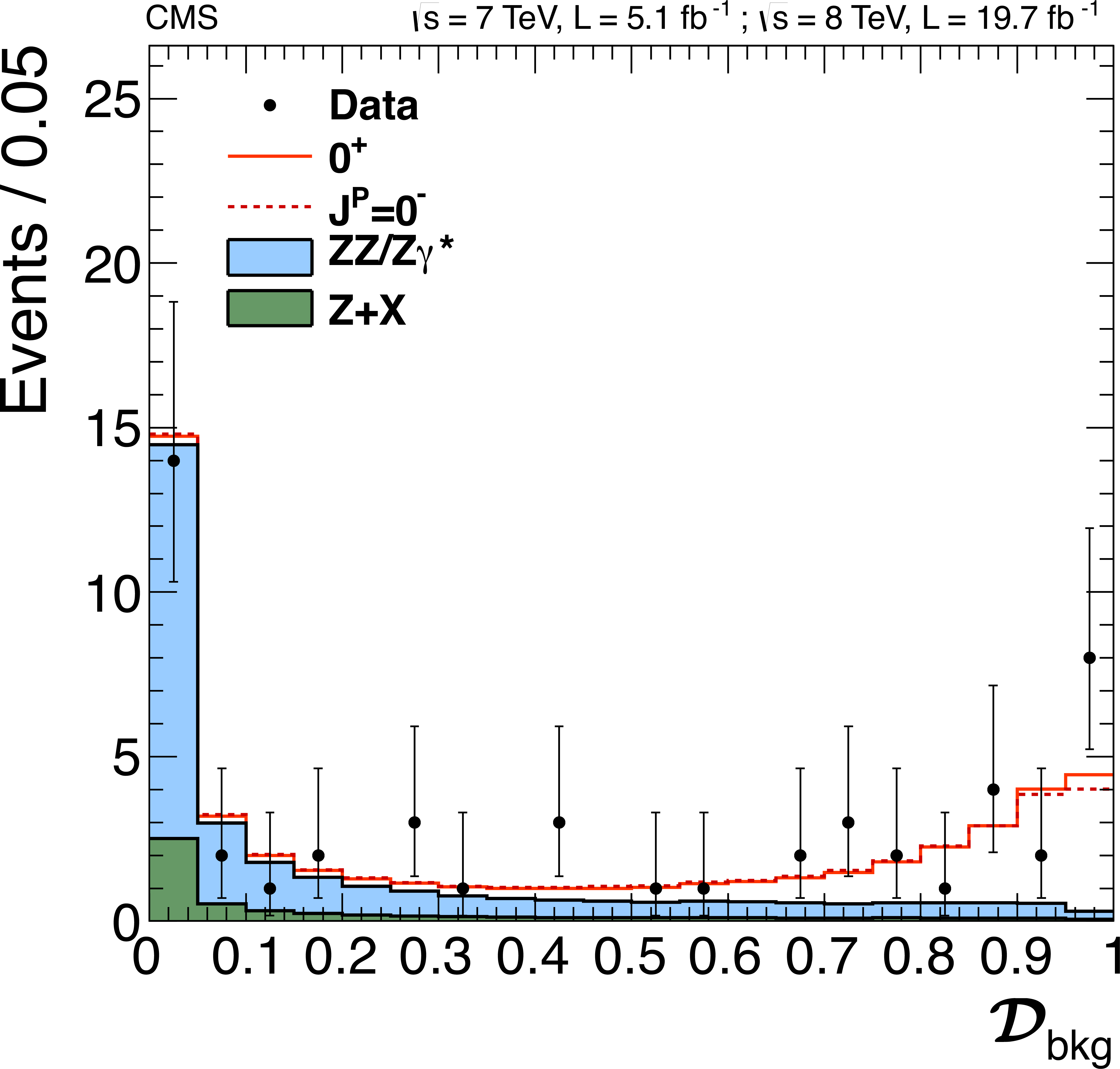
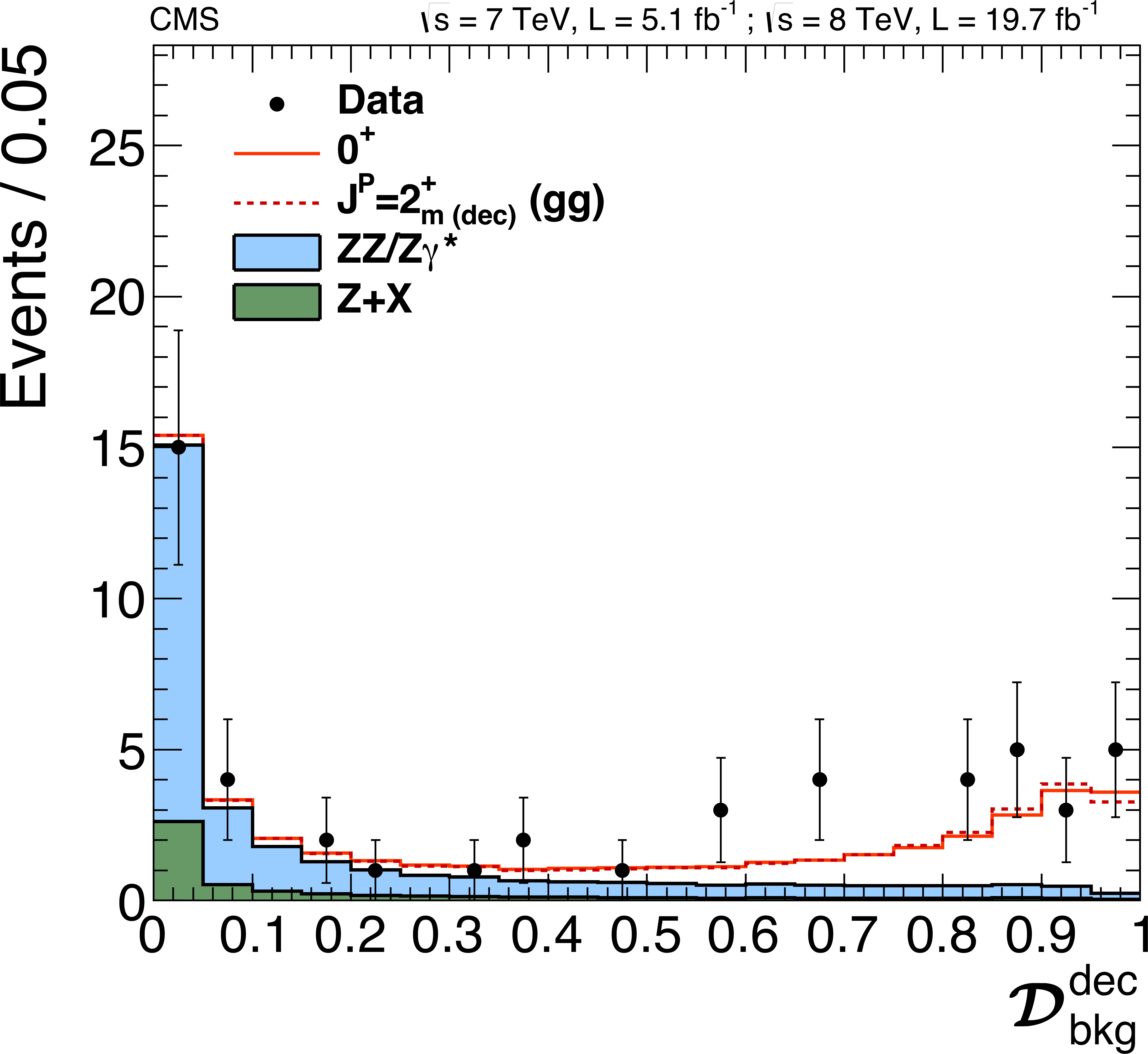
png pdf	Figure 23-a: Distribution of $ {\mathcal {D}_\text {bkg}} $ (a) and $\mathcal {D}_\text {bkg}^\text {dec}$ for the production-independent scenario (b) in data and MC expectations for the background and for a signal resonance consistent with the SM Higgs boson with $m_{0^+}$ = 125.6 GeV
png pdf	Figure 23-b: Distribution of $ {\mathcal {D}_\text {bkg}} $ (a) and $\mathcal {D}_\text {bkg}^\text {dec}$ for the production-independent scenario (b) in data and MC expectations for the background and for a signal resonance consistent with the SM Higgs boson with $m_{0^+}$ = 125.6 GeV
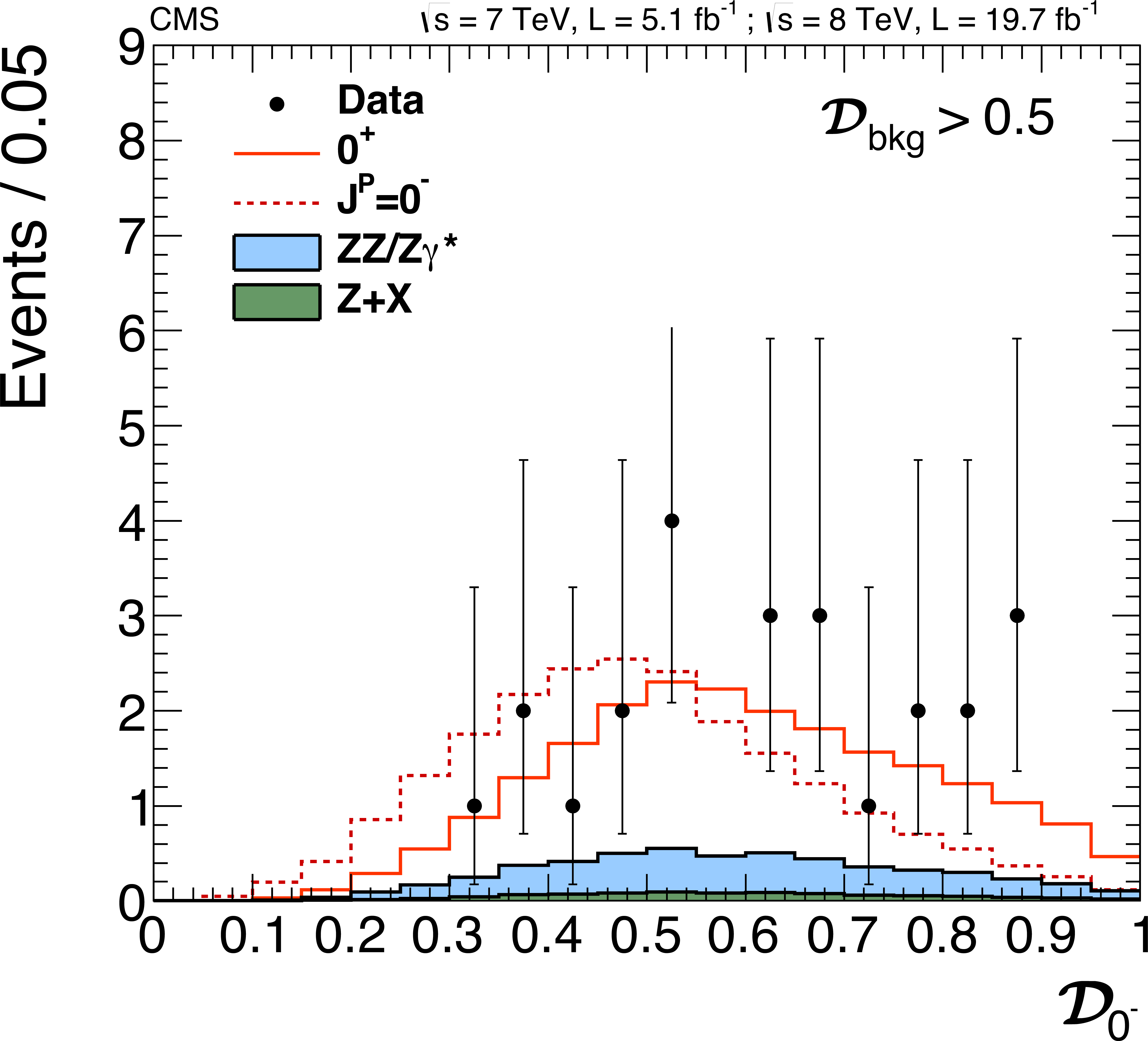
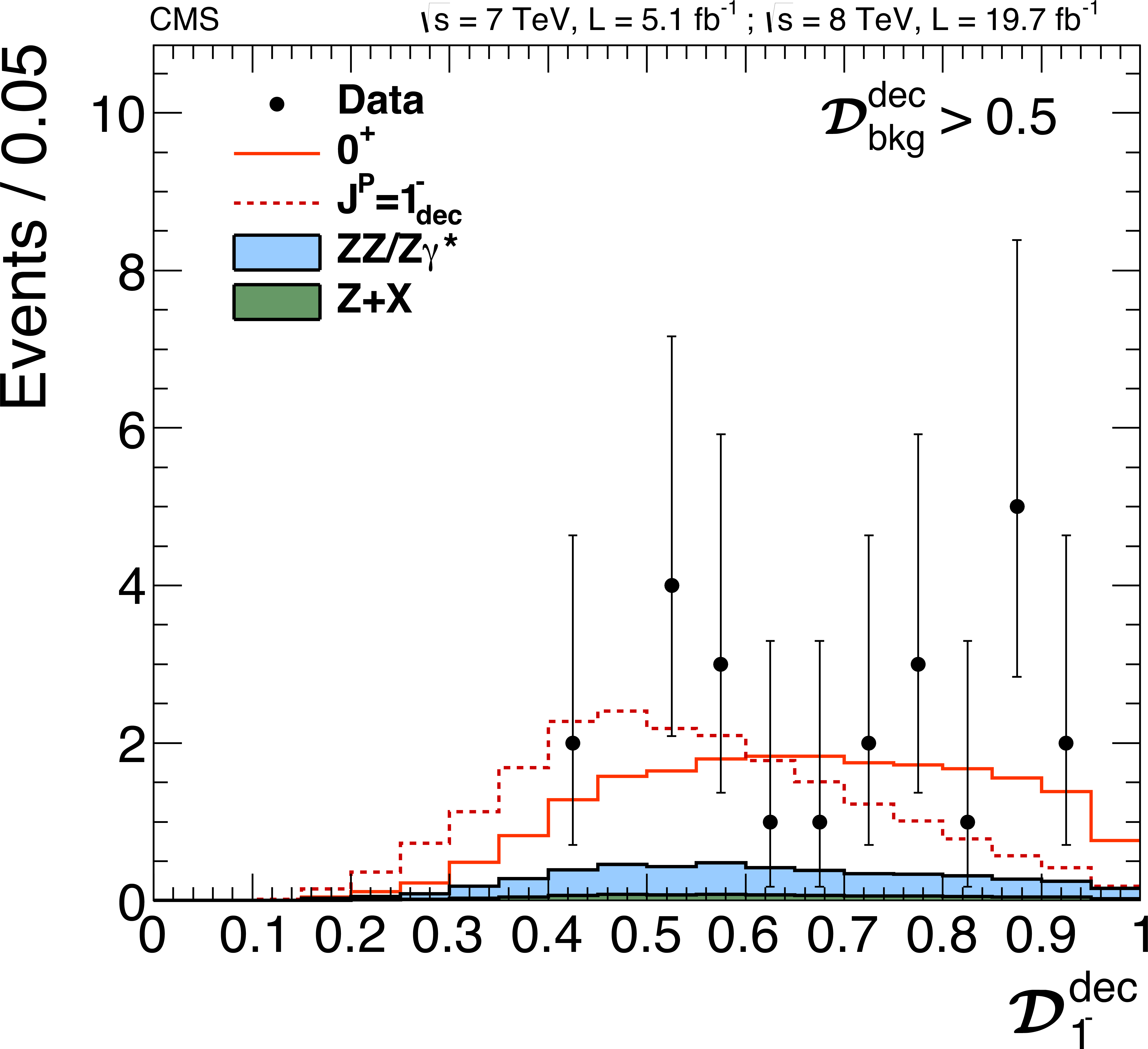
png pdf	Figure 24-a: Distributions of $ {\mathcal {D}_{J^P}} $ with a requirement $\mathcal {D}_\text {bkg}^\text {(dec)} > $ 0.5. Distributions in data (points with error bars) and expectations for background and signal are shown: six alternative $J^P$ hypotheses are shown. $J^P=0^-$ (a), $0_\mathrm {h}^+$ (b), $1^-( {\mathrm {q}} {\mathrm {\overline {q}}})$ (c), $1^-$ (d), $1^+( {\mathrm {q}} {\mathrm {\overline {q}}})$ (e), $1^+$ (f).
png pdf	Figure 24-b: Distributions of $ {\mathcal {D}_{J^P}} $ with a requirement $\mathcal {D}_\text {bkg}^\text {(dec)} > $ 0.5. Distributions in data (points with error bars) and expectations for background and signal are shown: six alternative $J^P$ hypotheses are shown. $J^P=0^-$ (a), $0_\mathrm {h}^+$ (b), $1^-( {\mathrm {q}} {\mathrm {\overline {q}}})$ (c), $1^-$ (d), $1^+( {\mathrm {q}} {\mathrm {\overline {q}}})$ (e), $1^+$ (f).
png pdf	Figure 24-c: Distributions of $ {\mathcal {D}_{J^P}} $ with a requirement $\mathcal {D}_\text {bkg}^\text {(dec)} > $ 0.5. Distributions in data (points with error bars) and expectations for background and signal are shown: six alternative $J^P$ hypotheses are shown. $J^P=0^-$ (a), $0_\mathrm {h}^+$ (b), $1^-( {\mathrm {q}} {\mathrm {\overline {q}}})$ (c), $1^-$ (d), $1^+( {\mathrm {q}} {\mathrm {\overline {q}}})$ (e), $1^+$ (f).
png pdf	Figure 24-d: Distributions of $ {\mathcal {D}_{J^P}} $ with a requirement $\mathcal {D}_\text {bkg}^\text {(dec)} > $ 0.5. Distributions in data (points with error bars) and expectations for background and signal are shown: six alternative $J^P$ hypotheses are shown. $J^P=0^-$ (a), $0_\mathrm {h}^+$ (b), $1^-( {\mathrm {q}} {\mathrm {\overline {q}}})$ (c), $1^-$ (d), $1^+( {\mathrm {q}} {\mathrm {\overline {q}}})$ (e), $1^+$ (f).
png pdf	Figure 24-e: Distributions of $ {\mathcal {D}_{J^P}} $ with a requirement $\mathcal {D}_\text {bkg}^\text {(dec)} > $ 0.5. Distributions in data (points with error bars) and expectations for background and signal are shown: six alternative $J^P$ hypotheses are shown. $J^P=0^-$ (a), $0_\mathrm {h}^+$ (b), $1^-( {\mathrm {q}} {\mathrm {\overline {q}}})$ (c), $1^-$ (d), $1^+( {\mathrm {q}} {\mathrm {\overline {q}}})$ (e), $1^+$ (f).
png pdf	Figure 24-f: Distributions of $ {\mathcal {D}_{J^P}} $ with a requirement $\mathcal {D}_\text {bkg}^\text {(dec)} > $ 0.5. Distributions in data (points with error bars) and expectations for background and signal are shown: six alternative $J^P$ hypotheses are shown. $J^P=0^-$ (a), $0_\mathrm {h}^+$ (b), $1^-( {\mathrm {q}} {\mathrm {\overline {q}}})$ (c), $1^-$ (d), $1^+( {\mathrm {q}} {\mathrm {\overline {q}}})$ (e), $1^+$ (f).
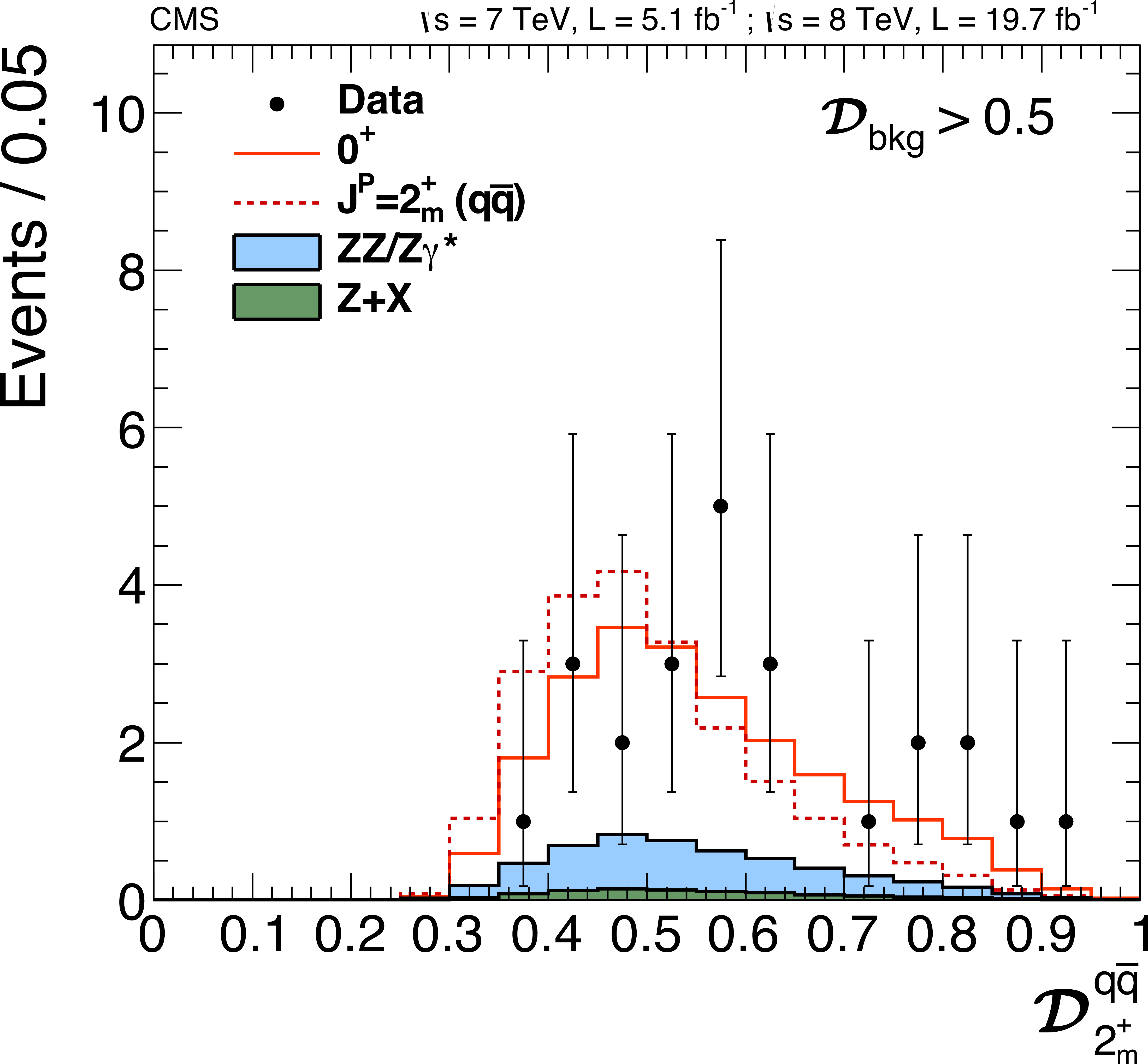
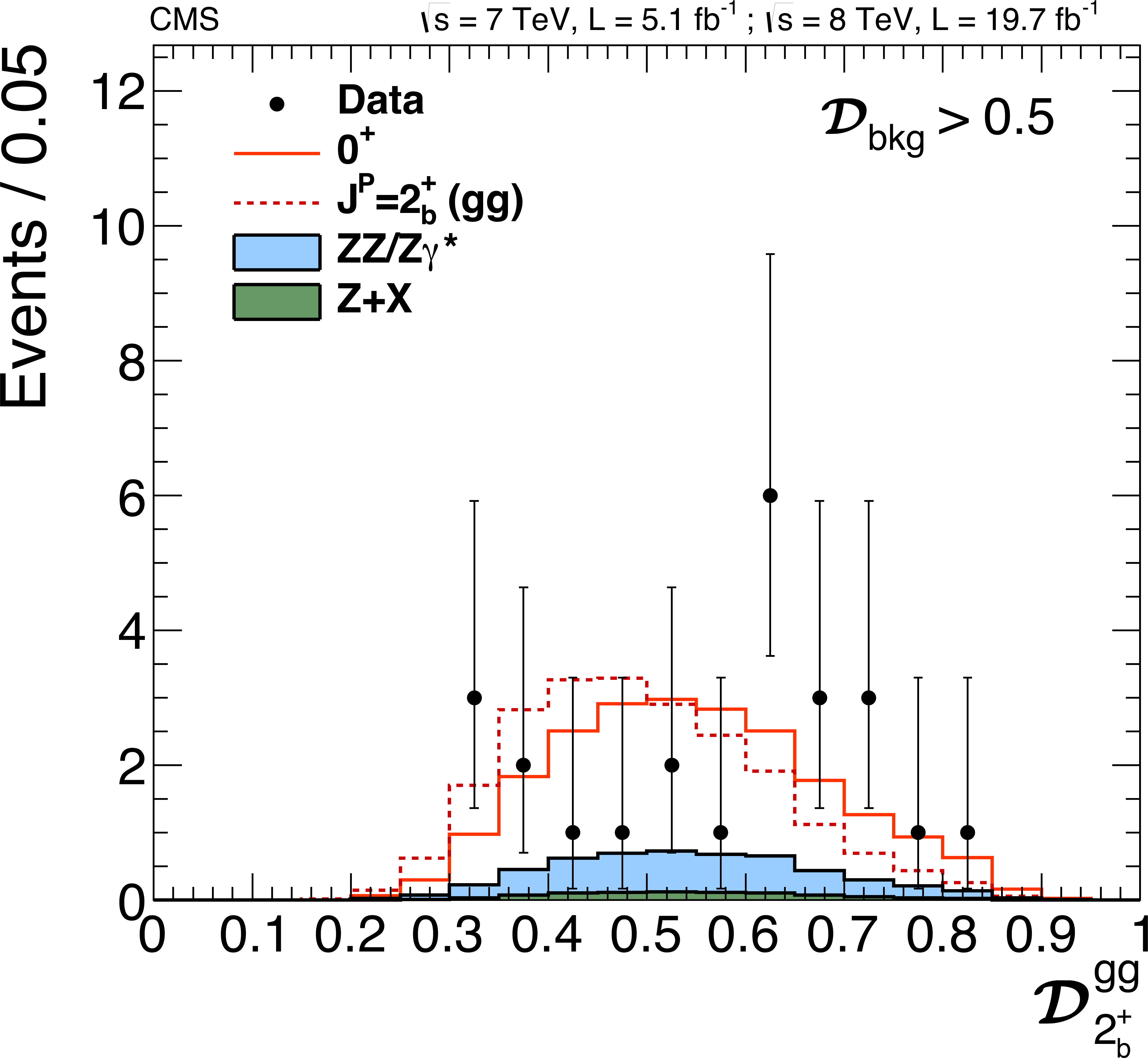
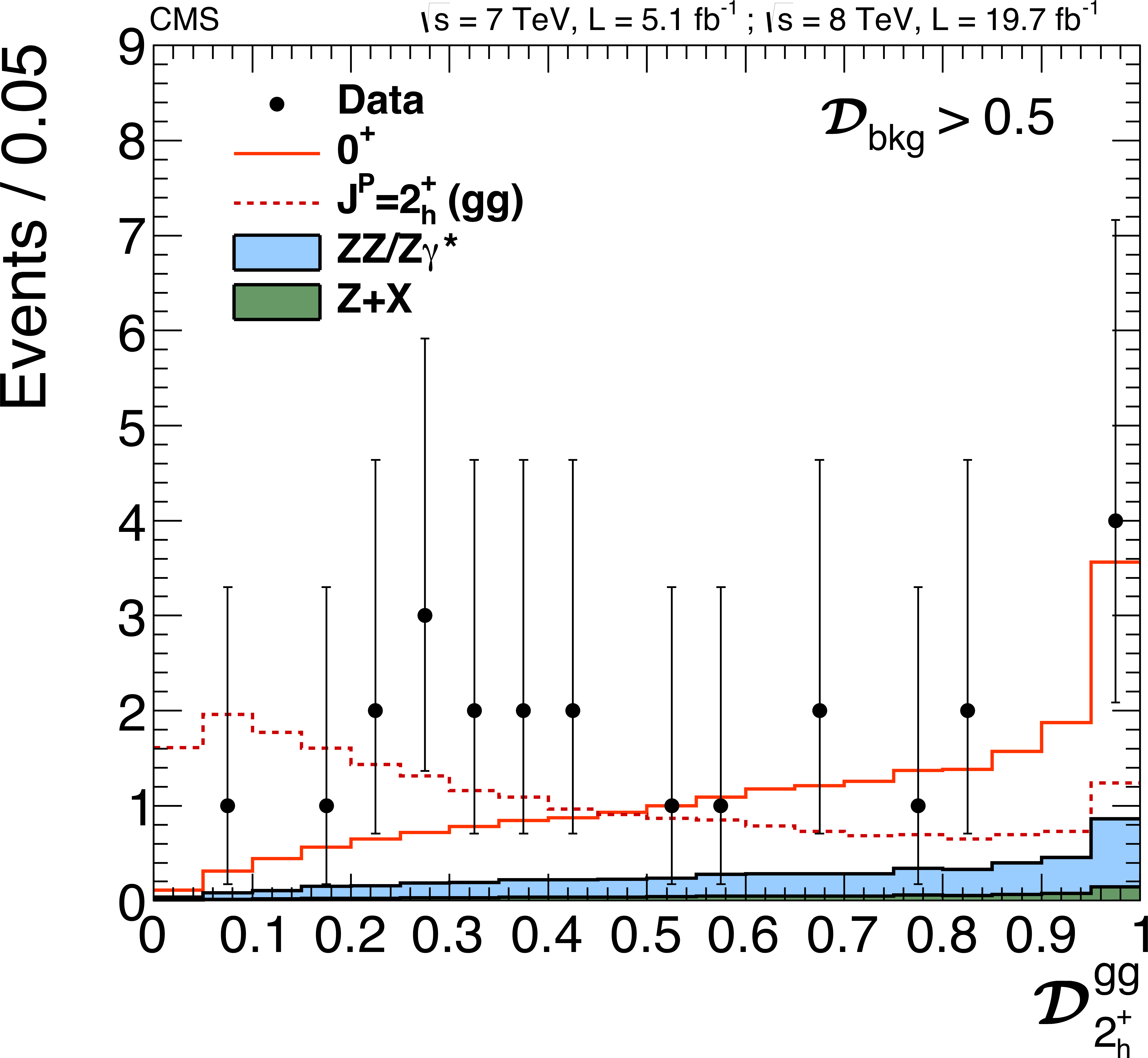
png pdf	Figure 25-a: Distributions of $ {\mathcal {D}_{J^P}} $ with a requirement $\mathcal {D}_\text {bkg}^\text {(dec)} > $ 0.5. Distributions in data (points with error bars) and expectations for background and signal are shown: six alternative $J^P$ hypotheses are shown. $J^P=2^{+}_\mathrm {m}$ for gluon fusion (a), $2^{+}_\mathrm {m}$ for VBF (b), $2^{+}_\mathrm {m}$ for the production-independent scenario (c), $2_\mathrm {b}^+( {\mathrm {g}} {\mathrm {g}} )$ (d), $2_\mathrm {h}^+( {\mathrm {g}} {\mathrm {g}} )$, (e), $2_\mathrm {h}^-( {\mathrm {g}} {\mathrm {g}} )$ (f).
png pdf	Figure 25-b: Distributions of $ {\mathcal {D}_{J^P}} $ with a requirement $\mathcal {D}_\text {bkg}^\text {(dec)} > $ 0.5. Distributions in data (points with error bars) and expectations for background and signal are shown: six alternative $J^P$ hypotheses are shown. $J^P=2^{+}_\mathrm {m}$ for gluon fusion (a), $2^{+}_\mathrm {m}$ for VBF (b), $2^{+}_\mathrm {m}$ for the production-independent scenario (c), $2_\mathrm {b}^+( {\mathrm {g}} {\mathrm {g}} )$ (d), $2_\mathrm {h}^+( {\mathrm {g}} {\mathrm {g}} )$, (e), $2_\mathrm {h}^-( {\mathrm {g}} {\mathrm {g}} )$ (f).
png pdf	Figure 25-c: Distributions of $ {\mathcal {D}_{J^P}} $ with a requirement $\mathcal {D}_\text {bkg}^\text {(dec)} > $ 0.5. Distributions in data (points with error bars) and expectations for background and signal are shown: six alternative $J^P$ hypotheses are shown. $J^P=2^{+}_\mathrm {m}$ for gluon fusion (a), $2^{+}_\mathrm {m}$ for VBF (b), $2^{+}_\mathrm {m}$ for the production-independent scenario (c), $2_\mathrm {b}^+( {\mathrm {g}} {\mathrm {g}} )$ (d), $2_\mathrm {h}^+( {\mathrm {g}} {\mathrm {g}} )$, (e), $2_\mathrm {h}^-( {\mathrm {g}} {\mathrm {g}} )$ (f).
png pdf	Figure 25-d: Distributions of $ {\mathcal {D}_{J^P}} $ with a requirement $\mathcal {D}_\text {bkg}^\text {(dec)} > $ 0.5. Distributions in data (points with error bars) and expectations for background and signal are shown: six alternative $J^P$ hypotheses are shown. $J^P=2^{+}_\mathrm {m}$ for gluon fusion (a), $2^{+}_\mathrm {m}$ for VBF (b), $2^{+}_\mathrm {m}$ for the production-independent scenario (c), $2_\mathrm {b}^+( {\mathrm {g}} {\mathrm {g}} )$ (d), $2_\mathrm {h}^+( {\mathrm {g}} {\mathrm {g}} )$, (e), $2_\mathrm {h}^-( {\mathrm {g}} {\mathrm {g}} )$ (f).
png pdf	Figure 25-e: Distributions of $ {\mathcal {D}_{J^P}} $ with a requirement $\mathcal {D}_\text {bkg}^\text {(dec)} > $ 0.5. Distributions in data (points with error bars) and expectations for background and signal are shown: six alternative $J^P$ hypotheses are shown. $J^P=2^{+}_\mathrm {m}$ for gluon fusion (a), $2^{+}_\mathrm {m}$ for VBF (b), $2^{+}_\mathrm {m}$ for the production-independent scenario (c), $2_\mathrm {b}^+( {\mathrm {g}} {\mathrm {g}} )$ (d), $2_\mathrm {h}^+( {\mathrm {g}} {\mathrm {g}} )$, (e), $2_\mathrm {h}^-( {\mathrm {g}} {\mathrm {g}} )$ (f).
png pdf	Figure 25-f: Distributions of $ {\mathcal {D}_{J^P}} $ with a requirement $\mathcal {D}_\text {bkg}^\text {(dec)} > $ 0.5. Distributions in data (points with error bars) and expectations for background and signal are shown: six alternative $J^P$ hypotheses are shown. $J^P=2^{+}_\mathrm {m}$ for gluon fusion (a), $2^{+}_\mathrm {m}$ for VBF (b), $2^{+}_\mathrm {m}$ for the production-independent scenario (c), $2_\mathrm {b}^+( {\mathrm {g}} {\mathrm {g}} )$ (d), $2_\mathrm {h}^+( {\mathrm {g}} {\mathrm {g}} )$, (e), $2_\mathrm {h}^-( {\mathrm {g}} {\mathrm {g}} )$ (f).
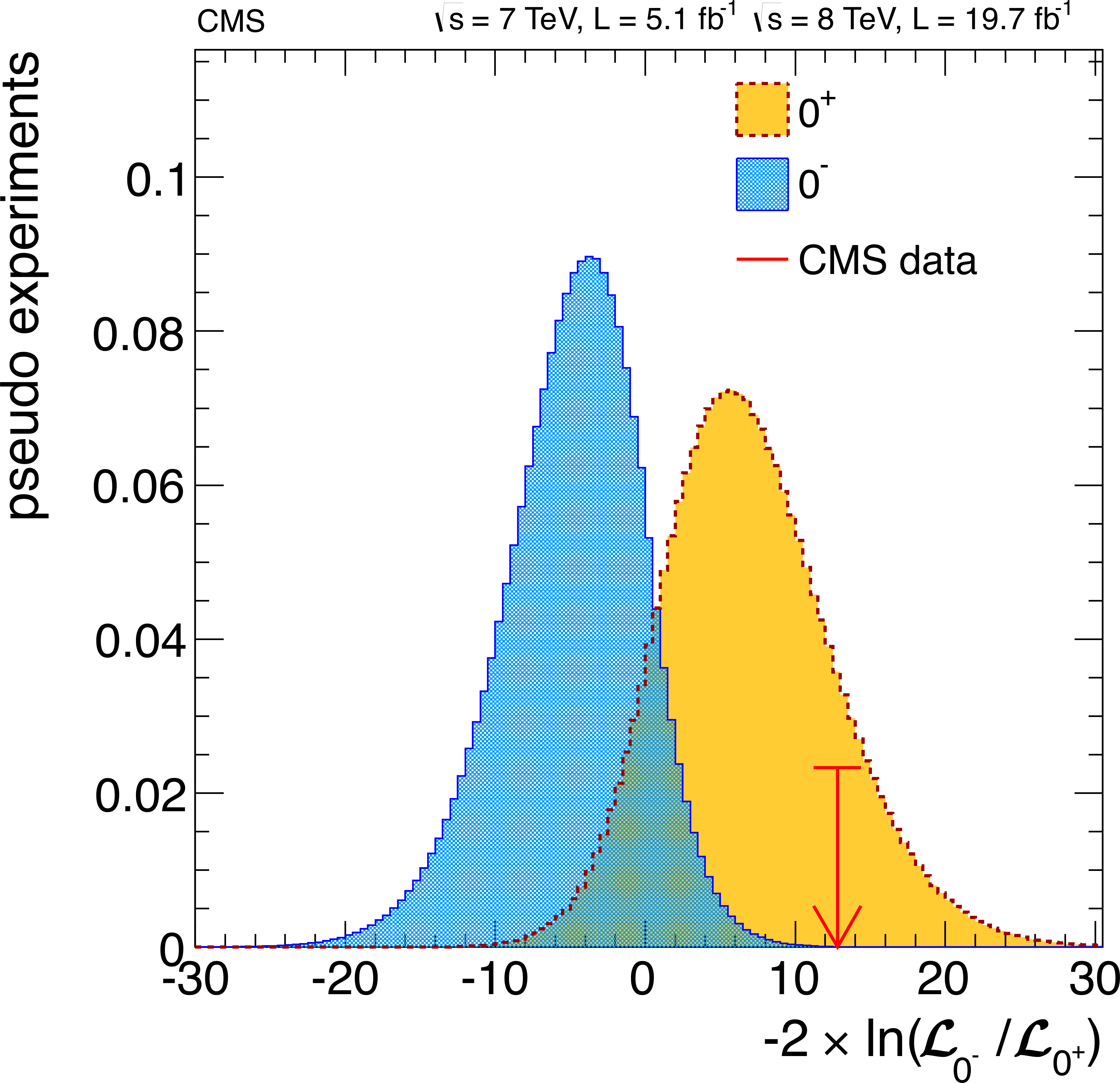
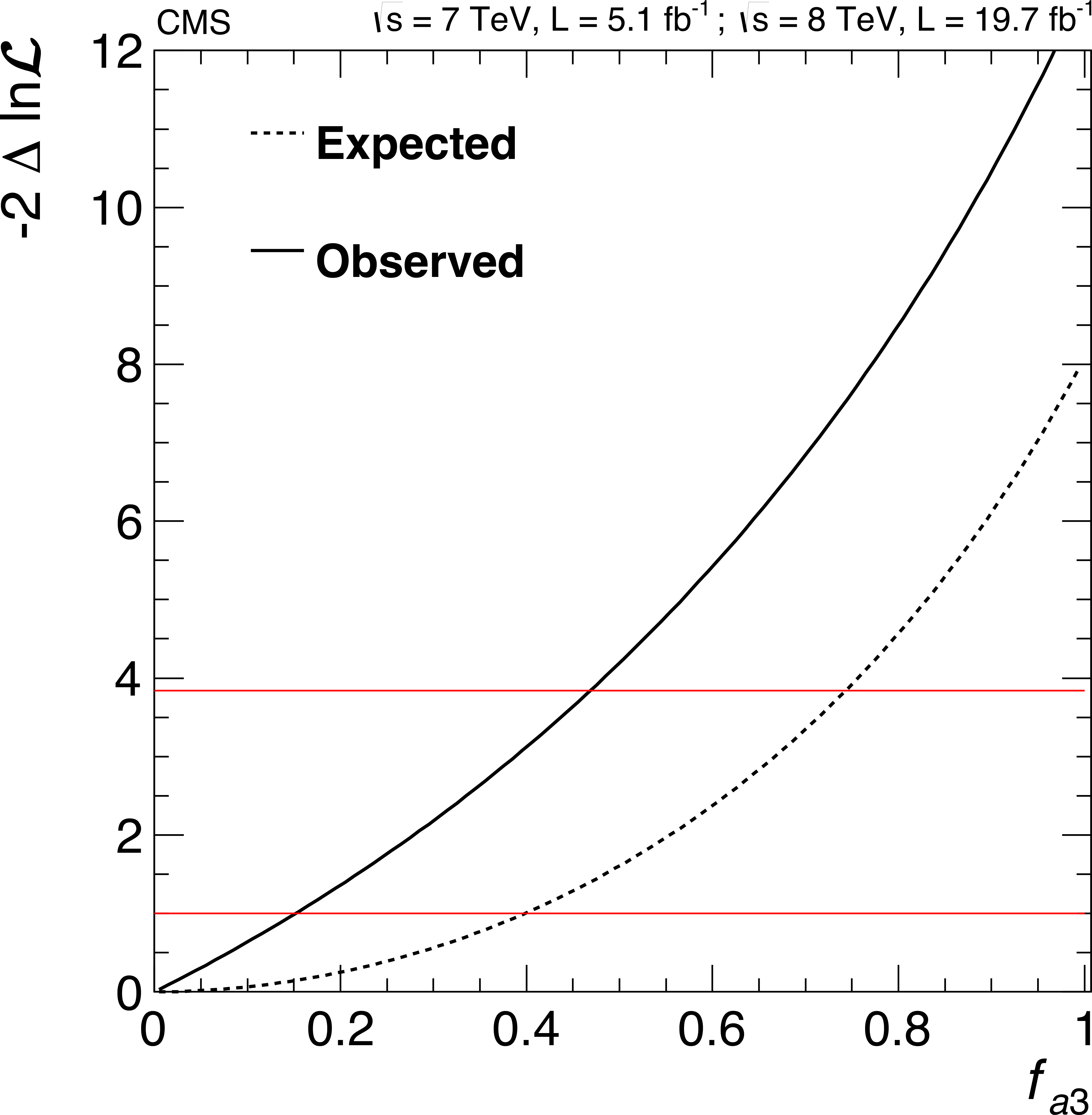
png pdf	Figure 26-a: (a) Distribution of the test statistic $q=-2 \ln (\mathcal {L}_{0^-}/\mathcal {L}_{0^+} ) $ of the pseudoscalar boson hypothesis tested against the SM Higgs boson hypothesis. Distributions for the SM Higgs boson are represented by the yellow histogram, and those for the alternative $J^P$ hypotheses are represented by the blue histogram. The arrow indicates the observed value. (b) Average expected and observed distribution of $-2\Delta \ln \mathcal{L}$ as a function of $f_{a3}$. The horizontal lines at $-2\Delta \ln{ \mathcal {L} }$ = 1 and 3.84 represent the 68% and 95% CL's, respectively.
png pdf	Figure 26-b: (a) Distribution of the test statistic $q=-2 \ln (\mathcal {L}_{0^-}/\mathcal {L}_{0^+} ) $ of the pseudoscalar boson hypothesis tested against the SM Higgs boson hypothesis. Distributions for the SM Higgs boson are represented by the yellow histogram, and those for the alternative $J^P$ hypotheses are represented by the blue histogram. The arrow indicates the observed value. (b) Average expected and observed distribution of $-2\Delta \ln \mathcal{L}$ as a function of $f_{a3}$. The horizontal lines at $-2\Delta \ln{ \mathcal {L} }$ = 1 and 3.84 represent the 68% and 95% CL's, respectively.
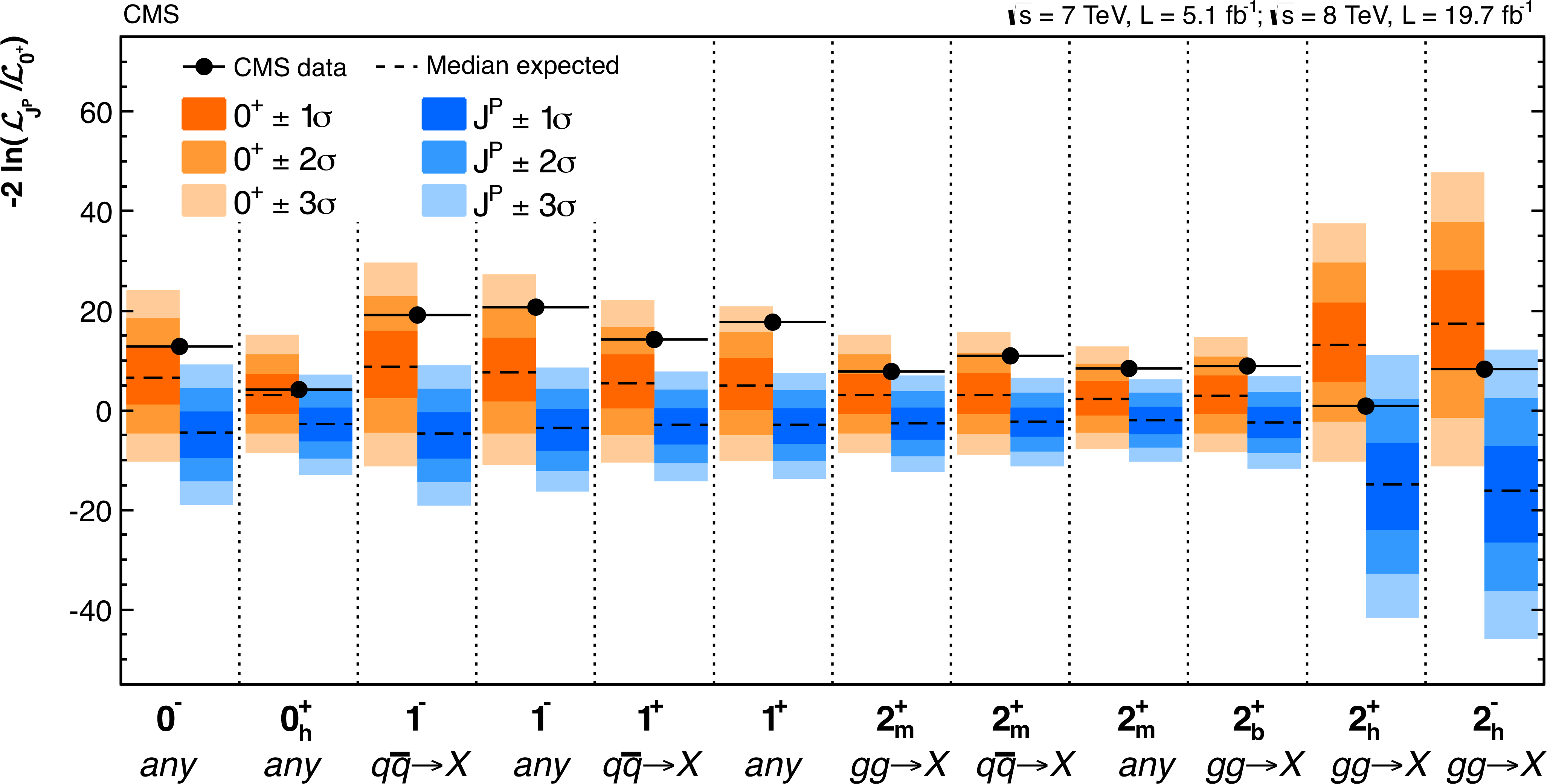
png pdf	Figure 27: Summary of the expected and observed values for the test-statistic $q$ distributions for the twelve alternative hypotheses tested with respect to the SM Higgs boson. The orange (blue) bands represent the 1$\sigma $, 2$\sigma $, and 3$\sigma $ around the median expected value for the SM Higgs boson hypothesis (alternative hypothesis). The black point represents the observed value.