

Compact Muon Solenoid
LHC, CERN
| CMS-HIG-13-004 ; CERN-PH-EP-2014-001 | ||
| Evidence for the 125 GeV Higgs boson decaying to a pair of $ \tau $ leptons | ||
| CMS Collaboration | ||
| 20 January 2014 | ||
| J. High Energy Phys. 05 (2014) 104 | ||
| Abstract: A search for a standard model Higgs boson decaying into a pair of tau leptons is performed using events recorded by the CMS experiment at the LHC in 2011 and 2012. The dataset corresponds to an integrated luminosity of 4.9 fb$ ^{-1}$ at a centre-of-mass energy of 7 TeV, and 19.7 fb$ ^{-1}$ at 8 TeV. Each tau lepton decays hadronically or leptonically to an electron or a muon, leading to six different final states for the tau-lepton pair, all considered in this analysis. An excess of events is observed over the expected background contributions, with a local significance larger than 3 standard deviations for $ m_{\mathrm{H}} $ values between 115 and 130 GeV. The best fit of the observed $ \mathrm{H} \to \tau \tau $ signal cross section for $ m_{\mathrm{H}} $ = 125 GeV is 0.78 $\pm$ 0.27 times the standard model expectation. These observations constitute evidence for the 125 GeV Higgs boson decaying to a pair of tau leptons. | ||
| Links: e-print arXiv:1401.5041 [hep-ex] (PDF) ; CDS record ; inSPIRE record ; Public twiki page ; CADI line (restricted) ; | ||
| Figures | |
png pdf |
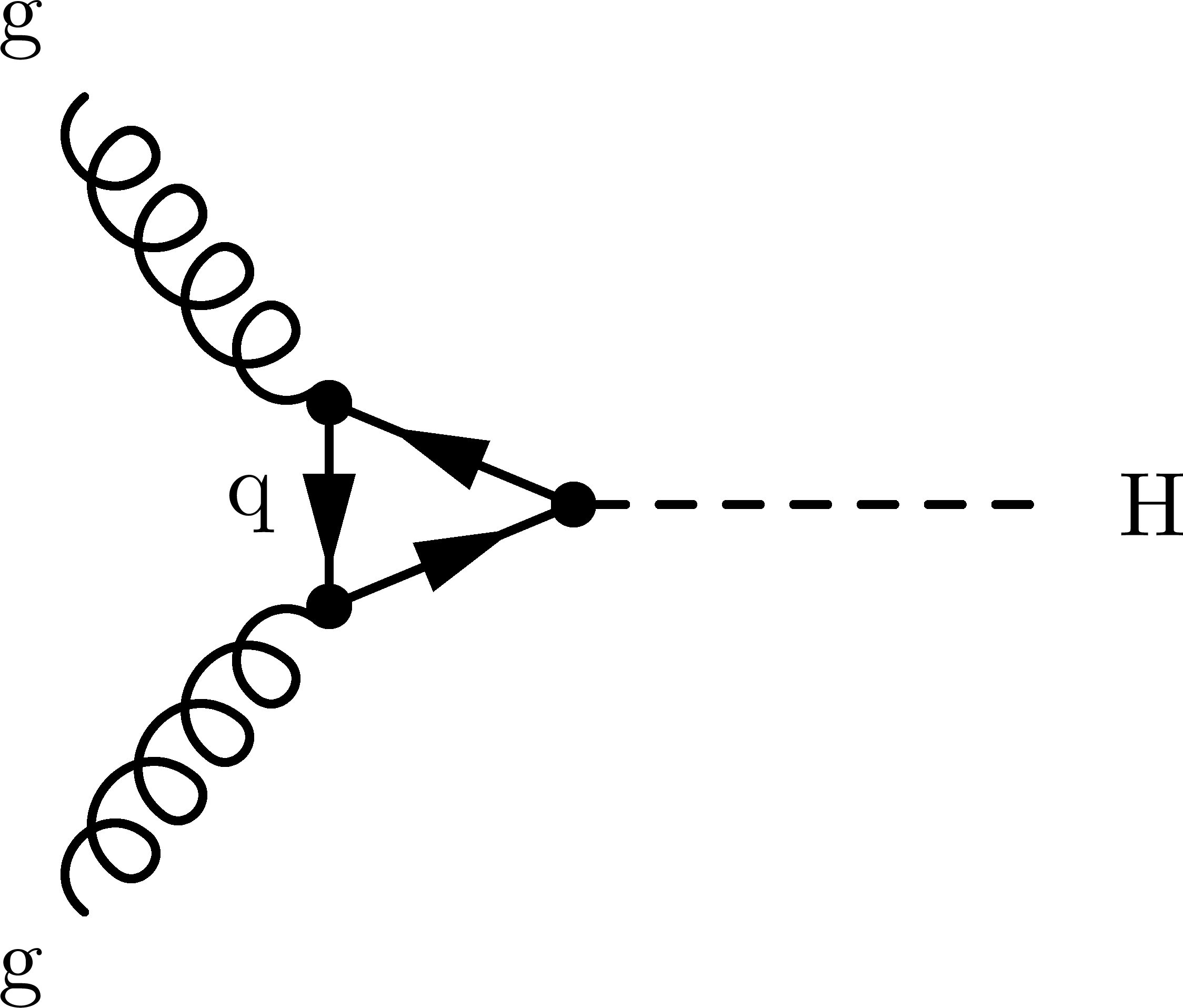
Figure 1-a:
Leading-order Feynman diagrams for Higgs boson production through gluon-gluon fusion (a), vector boson fusion (b), and the associated production with a $ {\mathrm {W}}$ or a $ {\mathrm {Z}}$ boson (c). |
png pdf |
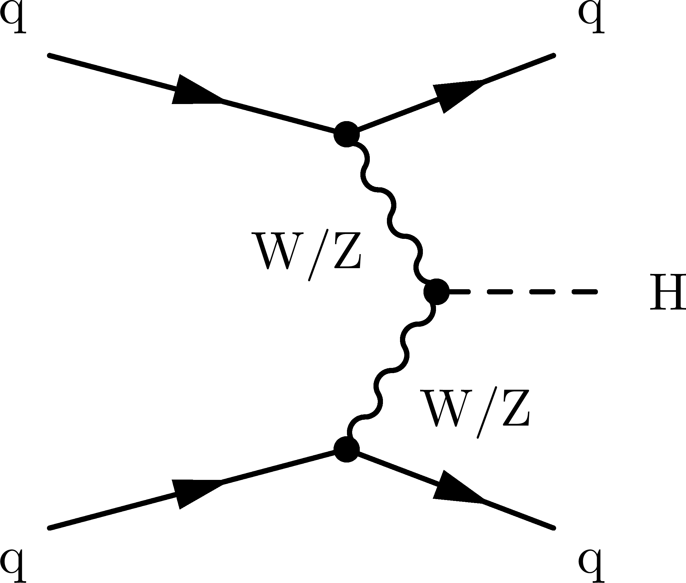
Figure 1-b:
Leading-order Feynman diagrams for Higgs boson production through gluon-gluon fusion (a), vector boson fusion (b), and the associated production with a $ {\mathrm {W}}$ or a $ {\mathrm {Z}}$ boson (c). |
png pdf |
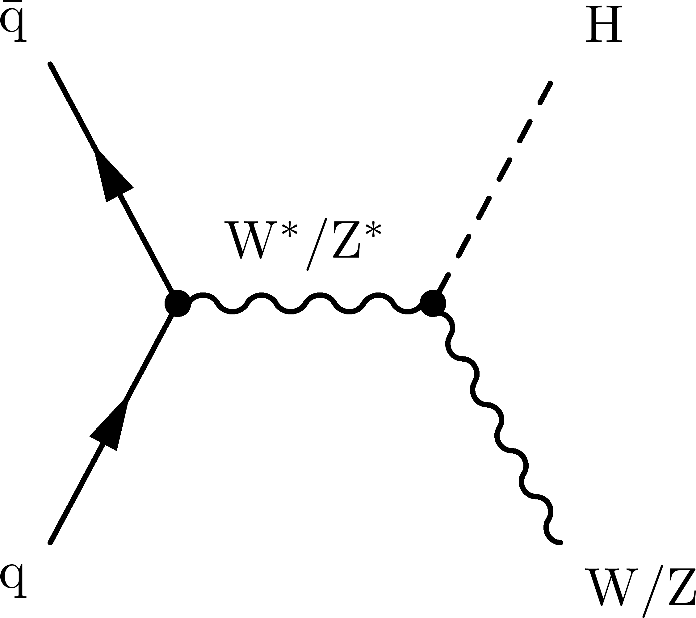
Figure 1-c:
Leading-order Feynman diagrams for Higgs boson production through gluon-gluon fusion (a), vector boson fusion (b), and the associated production with a $ {\mathrm {W}}$ or a $ {\mathrm {Z}}$ boson (c). |
png pdf |
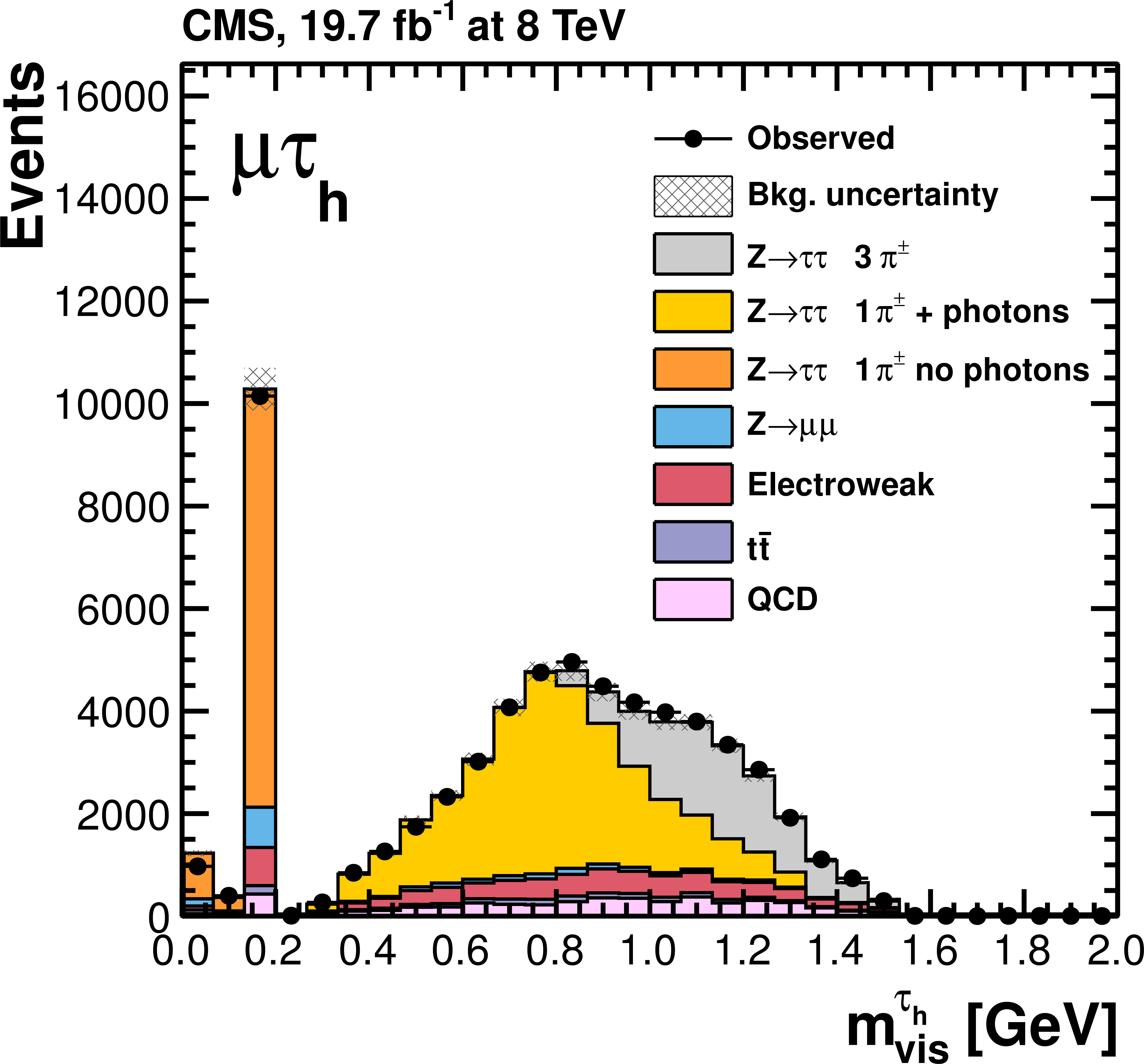
Figure 2:
Observed and predicted distributions for the visible $ { {\tau }_{\rm h}} $ mass, $ {m_\text {vis}} ^{ { {\tau }_{\rm h}} }$, in the $ {{\mu }} { {\tau }_{\rm h}} $ channel after the baseline selection described in section Event Selection. The yields predicted for the $ {\mathrm {Z}}\to \tau \tau $, $ {\mathrm {Z}}\to \mu \mu $, electroweak, $ {\mathrm {t}\overline {\mathrm {t}}} $, and QCD multijet background contributions correspond to the result of the final fit presented in Section Results. The $ {\mathrm {Z}}\to \tau \tau $ contribution is then split according to the decay mode reconstructed by the hadron-plus-strips algorithm as shown in the legend. The mass distribution of the $ { {\tau }_{\rm h}} $ built from one charged hadron and photons peaks near the mass of the intermediate $ {\rho \mathrm {(770)}}$ resonance; the mass distribution of the $ { {\tau }_{\rm h}} $ built from three charged hadrons peaks around the mass of the intermediate $ {\mathrm {a_1(1260)}}$ resonance. The $ { {\tau }_{\rm h}} $ built from one charged hadron and no photons are reconstructed with the $\pi ^\pm $ mass, assigned to all charged hadrons by the PF algorithm, and constitute the main contribution to the third bin of this histogram. The first two bins correspond to $\tau ^\pm $ leptons decaying into $ {\mathrm {e}}^\pm \nu \nu $ and $ {{\mu }}^\pm \nu \nu $, respectively, and for which the electron or muon is misidentified as a $ { {\tau }_{\rm h}} $. The electroweak background contribution is dominated by $ {\mathrm {W}}+\text {jets}$ production. In most selected $ {\mathrm {W}}+ \text {jets}$, $ {\mathrm {t}\overline {\mathrm {t}}} $, and QCD multijet events, a jet is misidentified as a $ { {\tau }_{\rm h}} $. The ``bkg. uncertainty'' band represents the combined statistical and systematic uncertainty in the background yield in each bin. The expected contribution from the SM Higgs signal is negligible. |
png pdf |
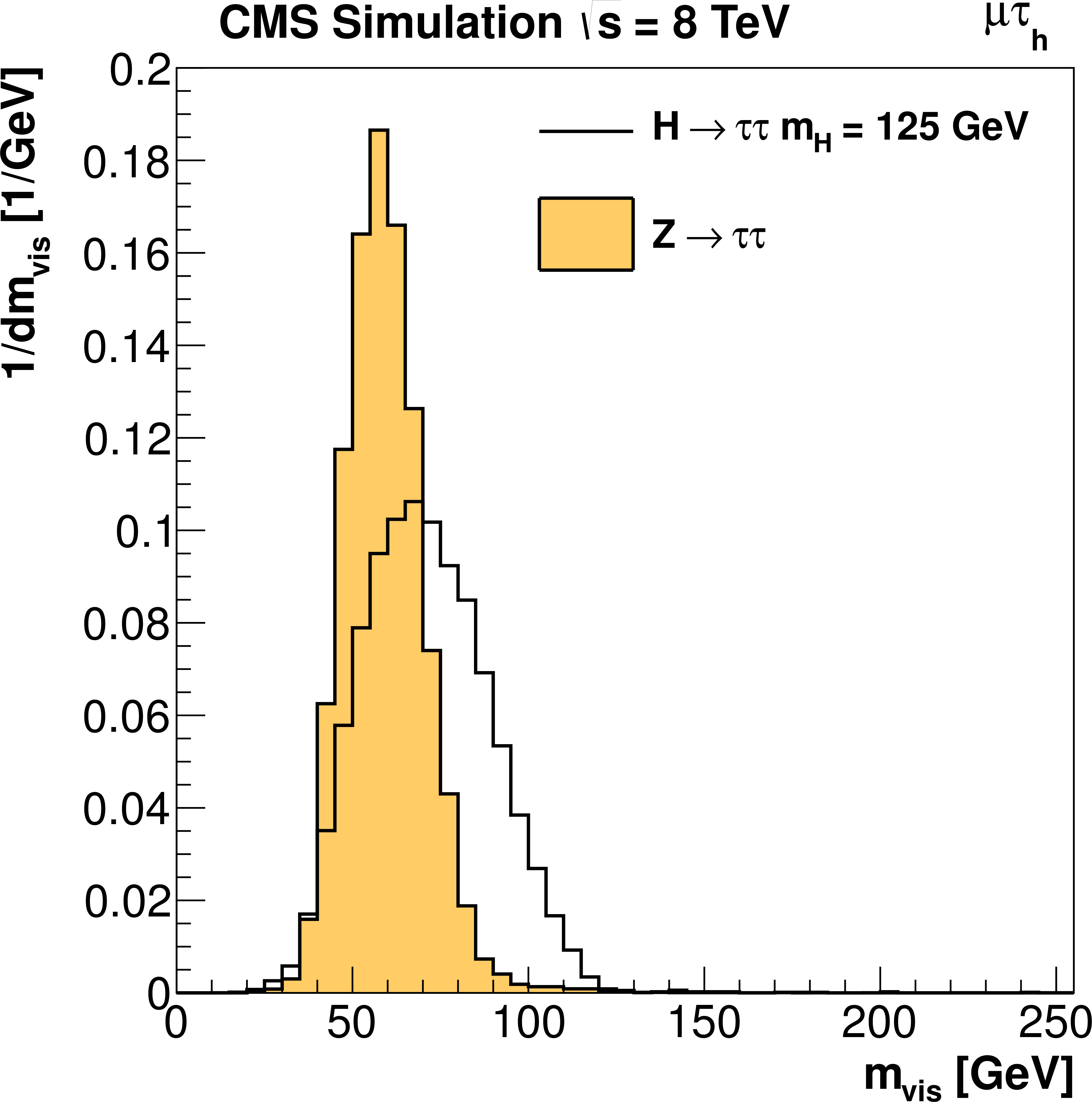
Figure 3-a:
Normalized distributions obtained in the $ {{\mu }} { {\tau }_{\rm h}} $ channel after the baseline selection for (a) the invariant mass, $ {m_\text {vis}} $, of the visible decay products of the two $\tau $ leptons, and (b) the \textsc {svfit} mass, $ {m_{ {\tau } {\tau }}} $. The distribution obtained for a simulated sample of $ {\mathrm {Z}}\to \tau \tau $ events (shaded histogram) is compared to the one obtained for a signal sample with a SM Higgs boson of mass $ {m_{ {\mathrm {H}} }}$ = 125 GeV (open histogram). |
png pdf |
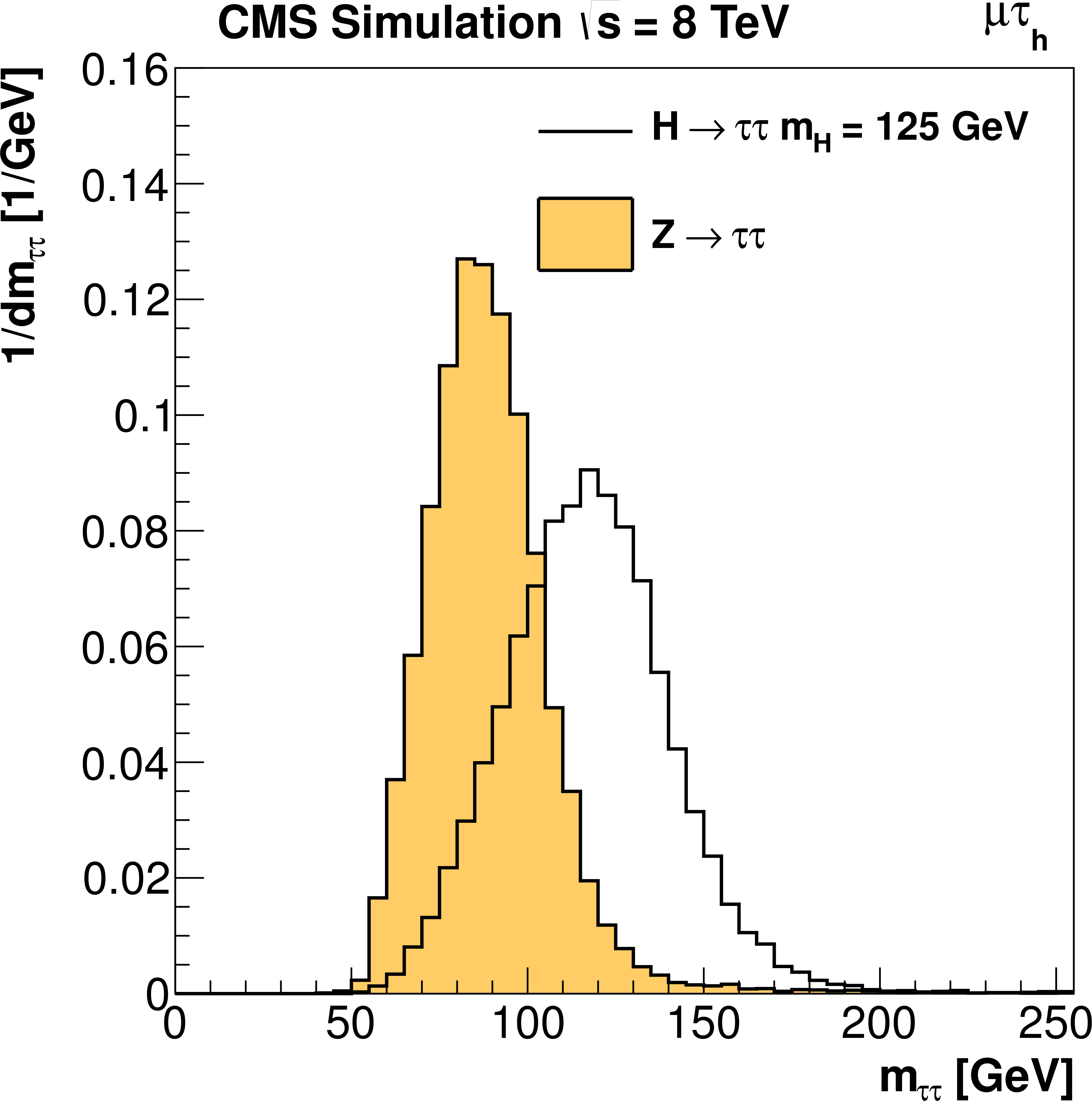
Figure 3-b:
Normalized distributions obtained in the $ {{\mu }} { {\tau }_{\rm h}} $ channel after the baseline selection for (a) the invariant mass, $ {m_\text {vis}} $, of the visible decay products of the two $\tau $ leptons, and (b) the \textsc {svfit} mass, $ {m_{ {\tau } {\tau }}} $. The distribution obtained for a simulated sample of $ {\mathrm {Z}}\to \tau \tau $ events (shaded histogram) is compared to the one obtained for a signal sample with a SM Higgs boson of mass $ {m_{ {\mathrm {H}} }}$ = 125 GeV (open histogram). |
png pdf |
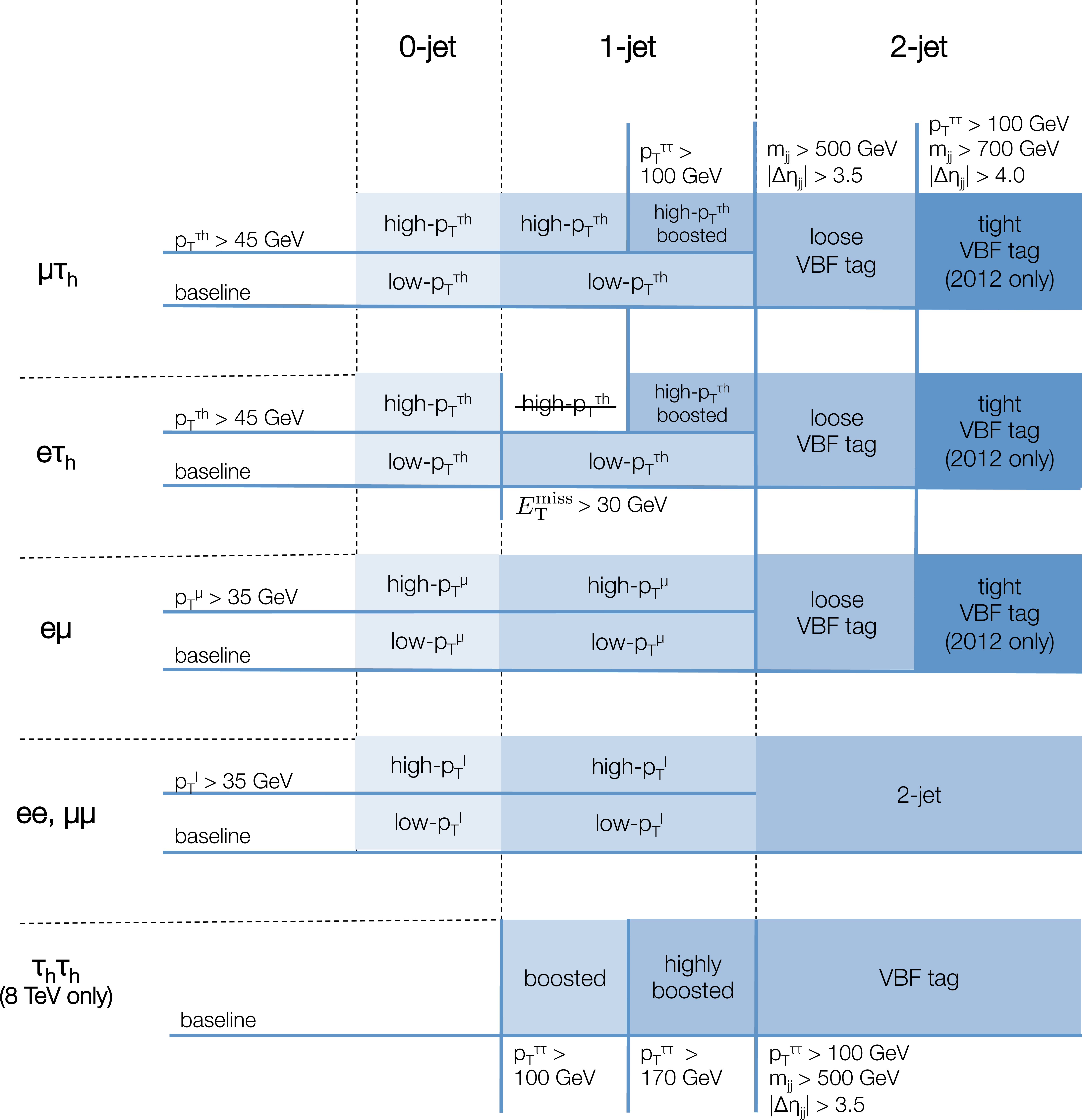
Figure 4:
Event categories for the $LL'$ channels. The $ { {p_{\mathrm {T}}} ^{\tau \tau }} $ variable is the transverse momentum of the Higgs boson candidate. In the definition of the VBF-tagged categories, $ {| {\Delta \eta _\mathrm {jj}} | }$ is the difference in pseudorapidity between the two highest-$p_{\mathrm {T}}$ jets, and $ {m_\mathrm {jj}} $ their invariant mass. In the $ {{\mu }} {{\mu }}$ and $ {\mathrm {e}} {\mathrm {e}}$ channels, events with two or more jets are not required to fulfil any additional VBF tagging criteria. For the analysis of the 7 TeV $ {\mathrm {e}} { {\tau }_{\rm h}} $ and $ {{\mu }} { {\tau }_{\rm h}} $ data, the loose and tight VBF-tagged categories are merged into a single VBF-tagged category. In the $ {\mathrm {e}} { {\tau }_{\rm h}} $ channel, the $E_{\mathrm {T}}^{\text {miss}}$ is required to be larger than 30 GeV in the 1-jet category. Therefore, the high-$ {p_{\mathrm {T}}} ^{ { {\tau }_{\rm h}} }$ category is not used and is accordingly crossed out. The term ``baseline'' refers to the baseline selection described in section Event Selection. |
png pdf |
Figure 5-a:
Observed and predicted distributions in the $ {{\mu }} { {\tau }_{\rm h}} $ channel after the baseline selection, for (a) the transverse momentum of the Higgs boson candidates and (b) the transverse momentum of the $ { {\tau }_{\rm h}} $. The yields predicted for the various background contributions correspond to the result of the final fit presented in Section {sec:results}. The electroweak background contribution includes events from $ {\mathrm {W}}+ \text {jets}$, diboson, and single-top-quark production. The ``bkg. uncertainty'' band represents the combined statistical and systematic uncertainty in the background yield in each bin. In each plot, the bottom inset shows the ratio of the observed and predicted numbers of events. The expected contribution from the SM Higgs signal is negligible. |
png pdf |
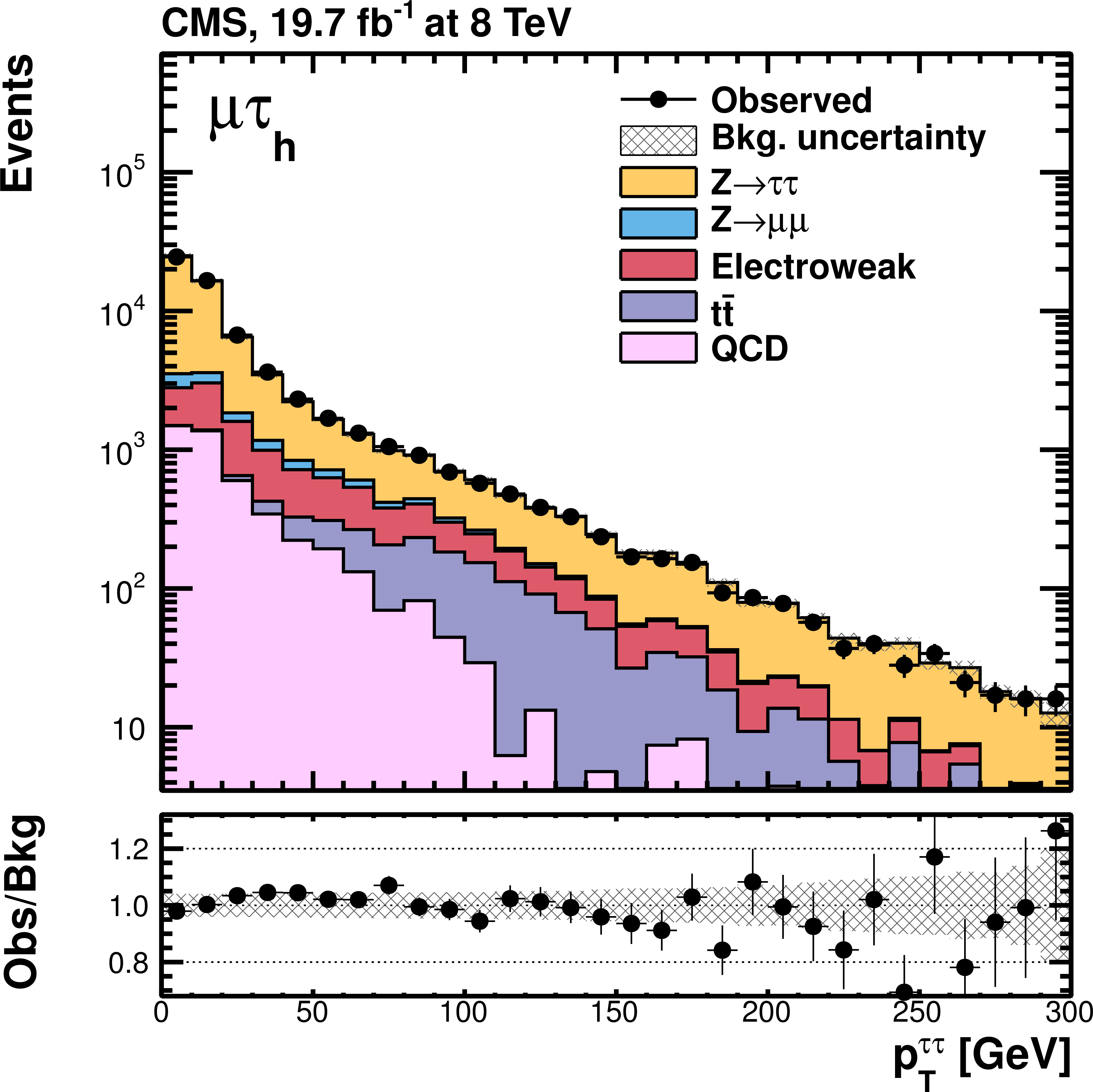
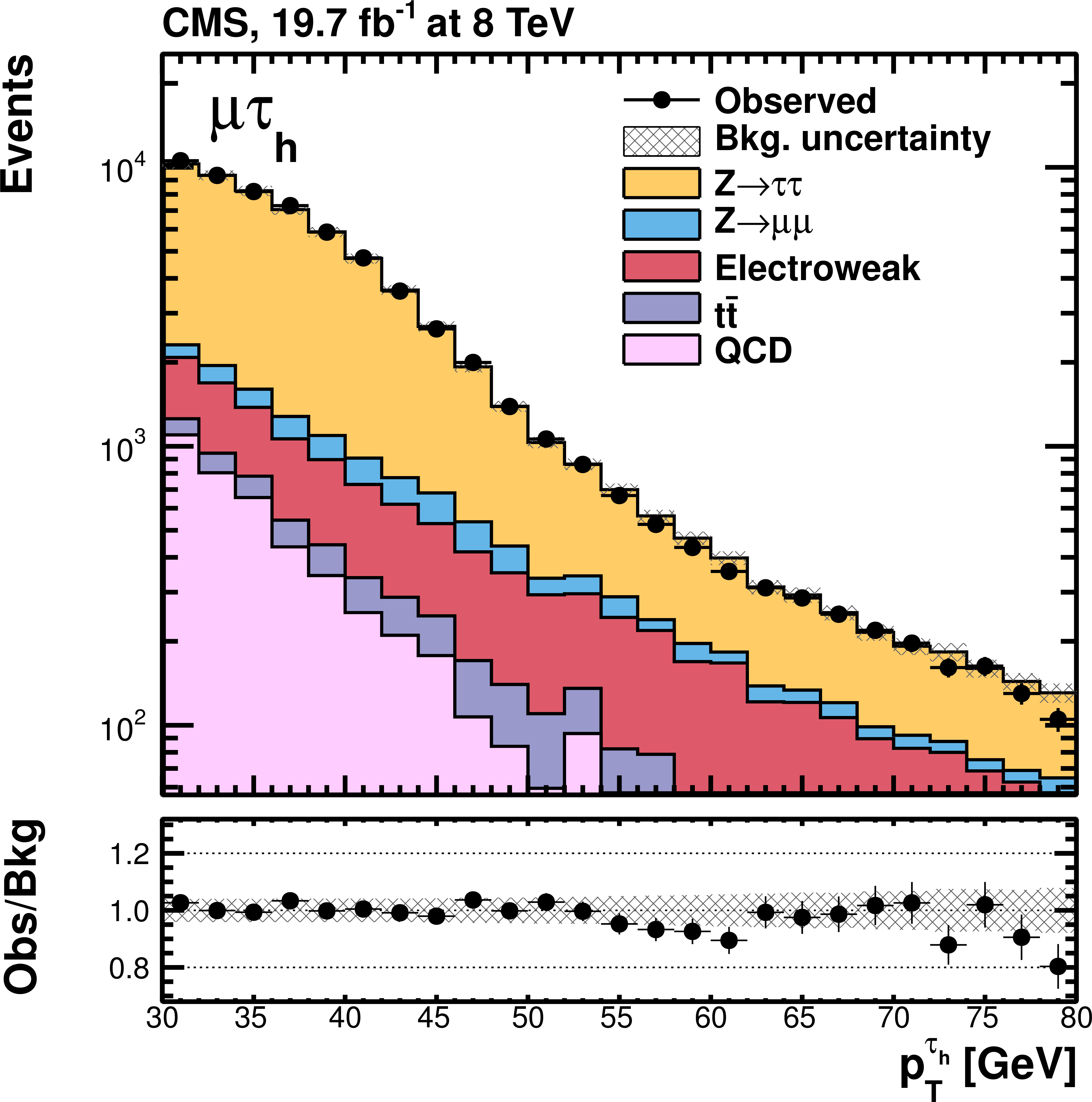
Figure 5-b:
Observed and predicted distributions in the $ {{\mu }} { {\tau }_{\rm h}} $ channel after the baseline selection, for (a) the transverse momentum of the Higgs boson candidates and (b) the transverse momentum of the $ { {\tau }_{\rm h}} $. The yields predicted for the various background contributions correspond to the result of the final fit presented in Section {sec:results}. The electroweak background contribution includes events from $ {\mathrm {W}}+ \text {jets}$, diboson, and single-top-quark production. The ``bkg. uncertainty'' band represents the combined statistical and systematic uncertainty in the background yield in each bin. In each plot, the bottom inset shows the ratio of the observed and predicted numbers of events. The expected contribution from the SM Higgs signal is negligible. |
png pdf |
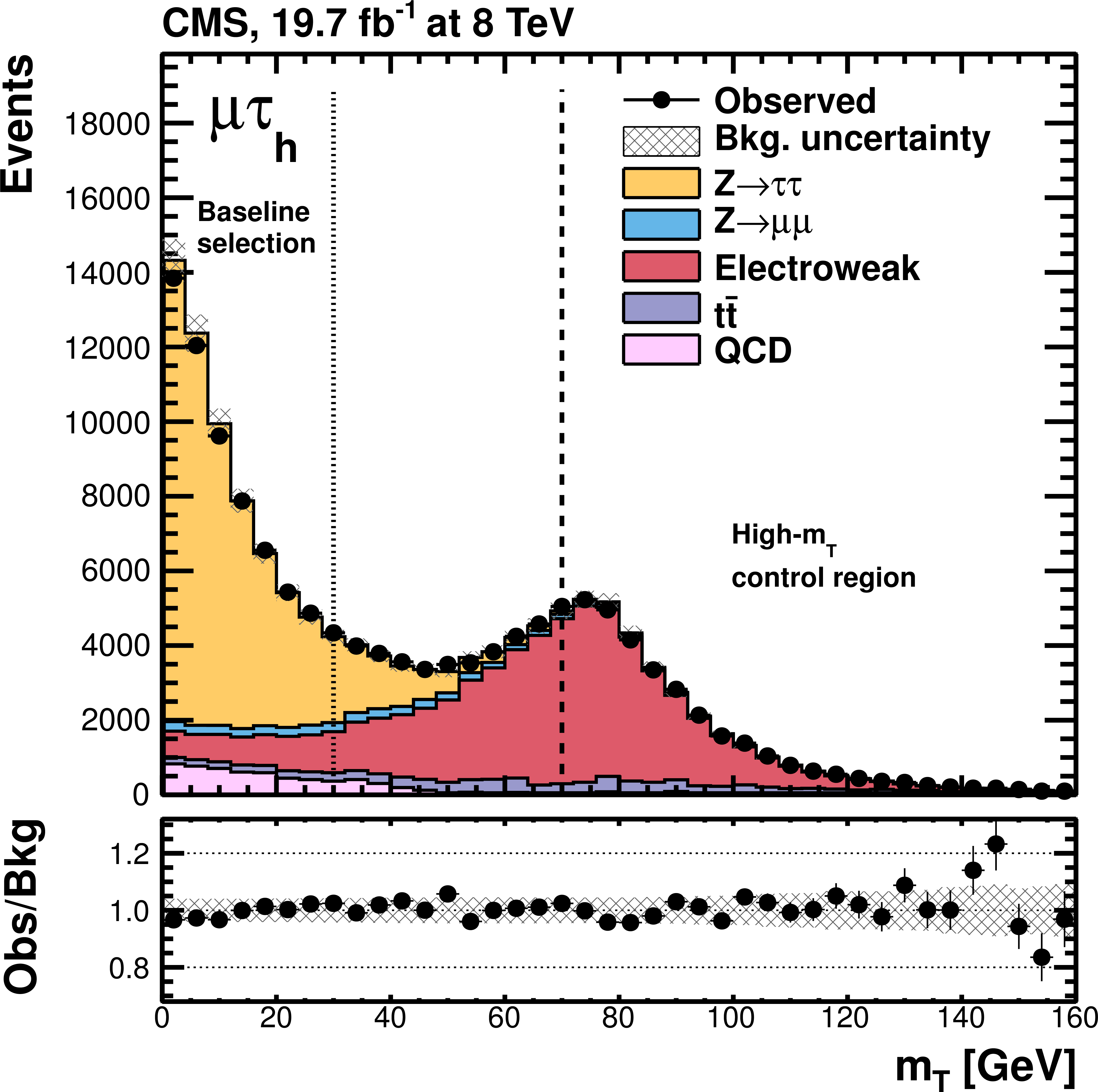
Figure 6:
Observed and predicted $ {m_\mathrm {T}} $ distribution in the 8 TeV $ {{\mu }} { {\tau }_{\rm h}} $ analysis after the baseline selection but before applying the $ {m_\mathrm {T}} < $ 30 GeV requirement, illustrated as a dotted vertical line. The dashed line delimits the high-$ {m_\mathrm {T}} $ control region that is used to normalize the yield of the $ {\mathrm {W}}+\text {jets}$ contribution in the analysis as described in the text. The yields predicted for the various background contributions correspond to the result of the final fit presented in Section {sec:results}. The electroweak background contribution includes events from $ {\mathrm {W}}+\text {jets}$, diboson, and single-top-quark production. The ``bkg. uncertainty'' band represents the combined statistical and systematic uncertainty in the background yield in each bin. The bottom inset shows the ratio of the observed and predicted numbers of events. The expected contribution from a SM Higgs signal is negligible. |
png pdf |
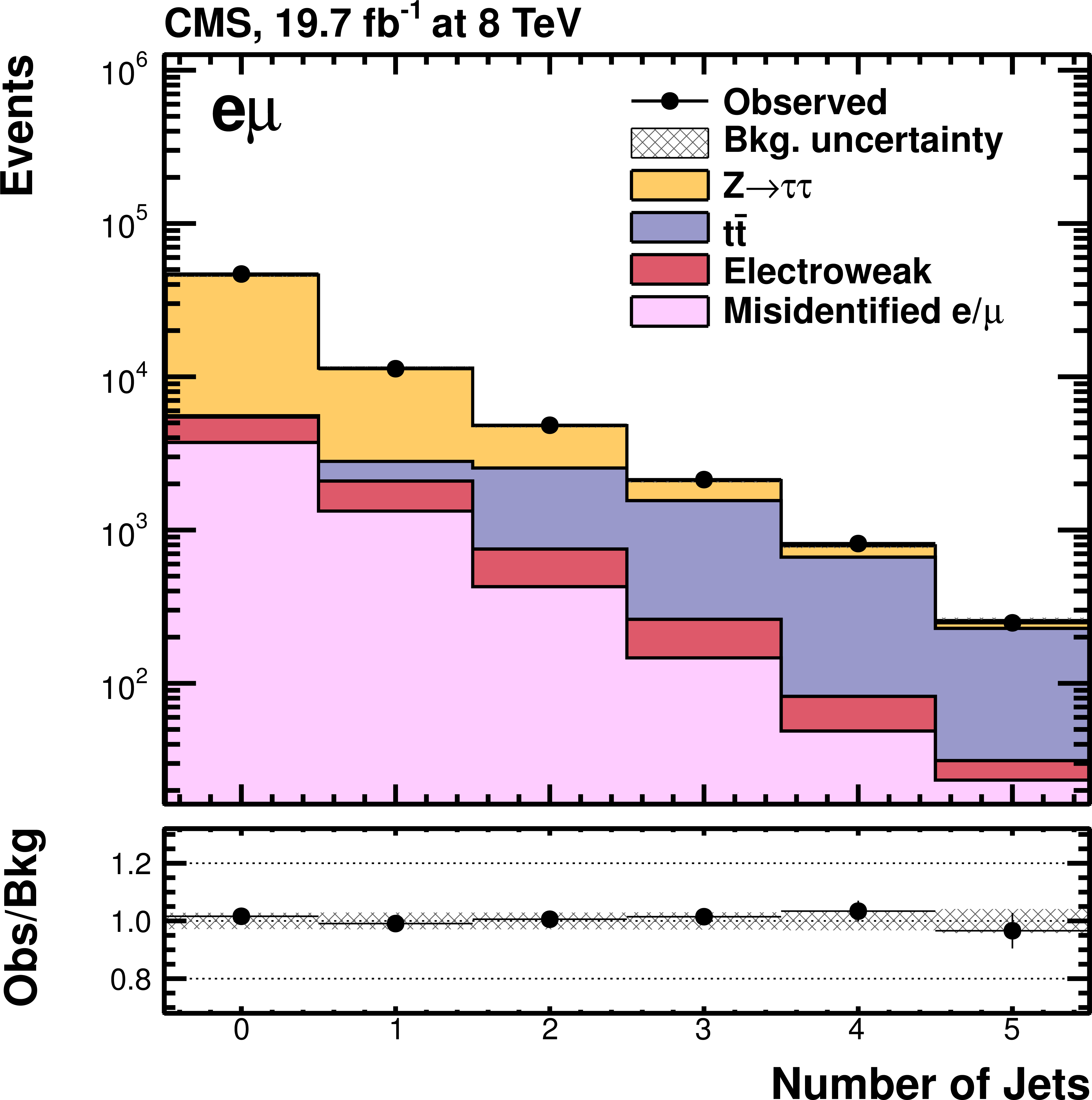
Figure 7:
Observed and predicted distribution for the number of jets in the 8 TeV $ {\mathrm {e}} {{\mu }}$ analysis after the baseline selection described in section Event Selection. The yields predicted for the various background contributions correspond to the result of the final fit presented in Section Results. The electroweak background contribution includes events from diboson and single-top-quark production. The ``bkg. uncertainty'' band represents the combined statistical and systematic uncertainty in the background yield in each bin. The bottom inset shows the ratio of the observed and predicted numbers of events. The expected contribution from a SM Higgs signal is negligible. |

png pdf |
Figure 8-a:
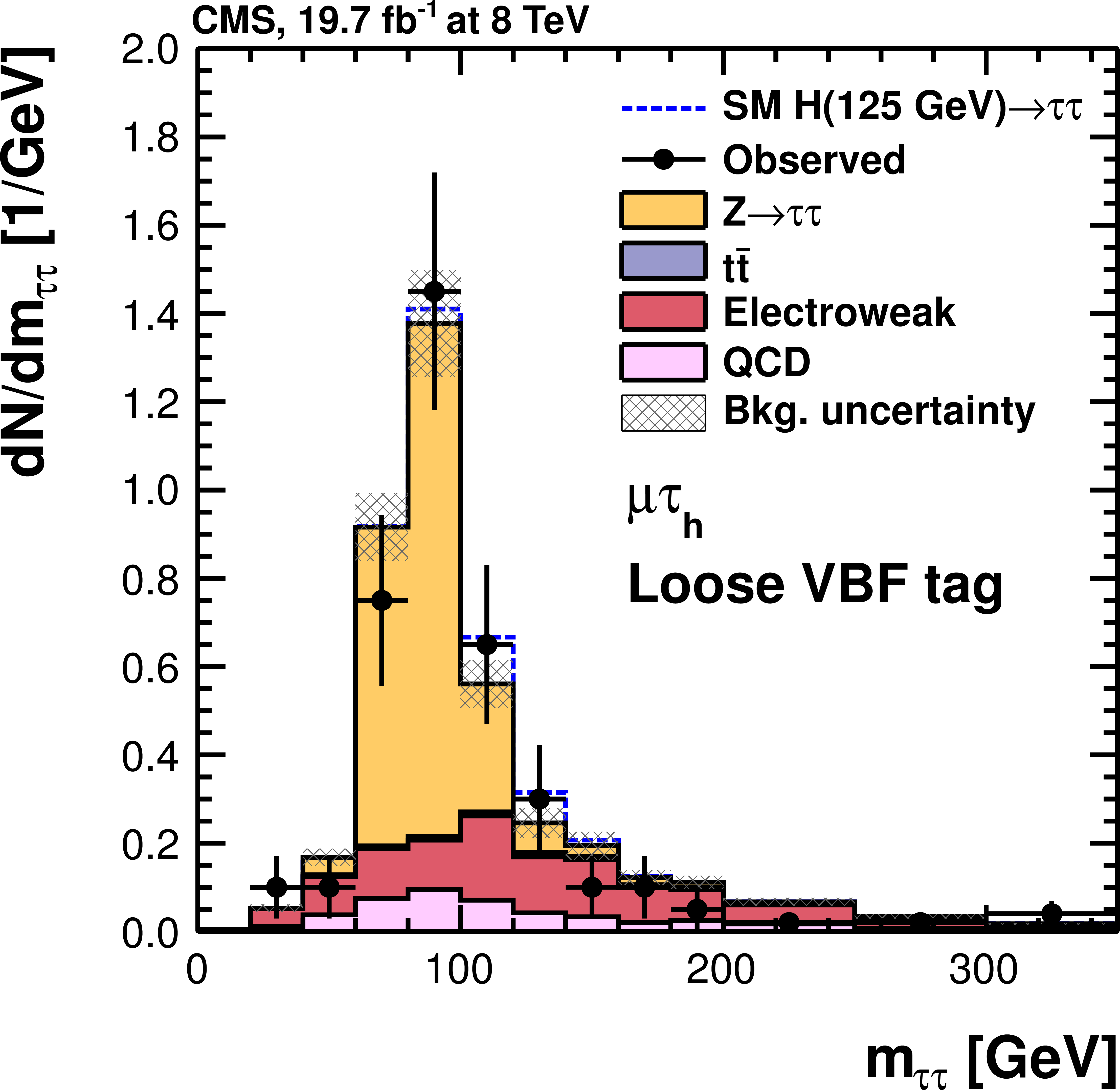
Observed and predicted $ {m_{ {\tau } {\tau }}} $ distributions in the 8 TeV $ {{\mu }} { {\tau }_{\rm h}} $ (a, c, e) and $e { {\tau }_{\rm h}} $ (b, d, f) channels, and for the 1-jet high-$ {p_{\mathrm {T}}} ^{ { {\tau }_{\rm h}} }$ boosted (a, b), loose VBF tag (c, d), and tight VBF tag (e, f) categories. The normalization of the predicted background distributions corresponds to the result of the global fit. The signal distribution, on the other hand, is normalized to the SM prediction. The signal and background histograms are stacked. |
png pdf |
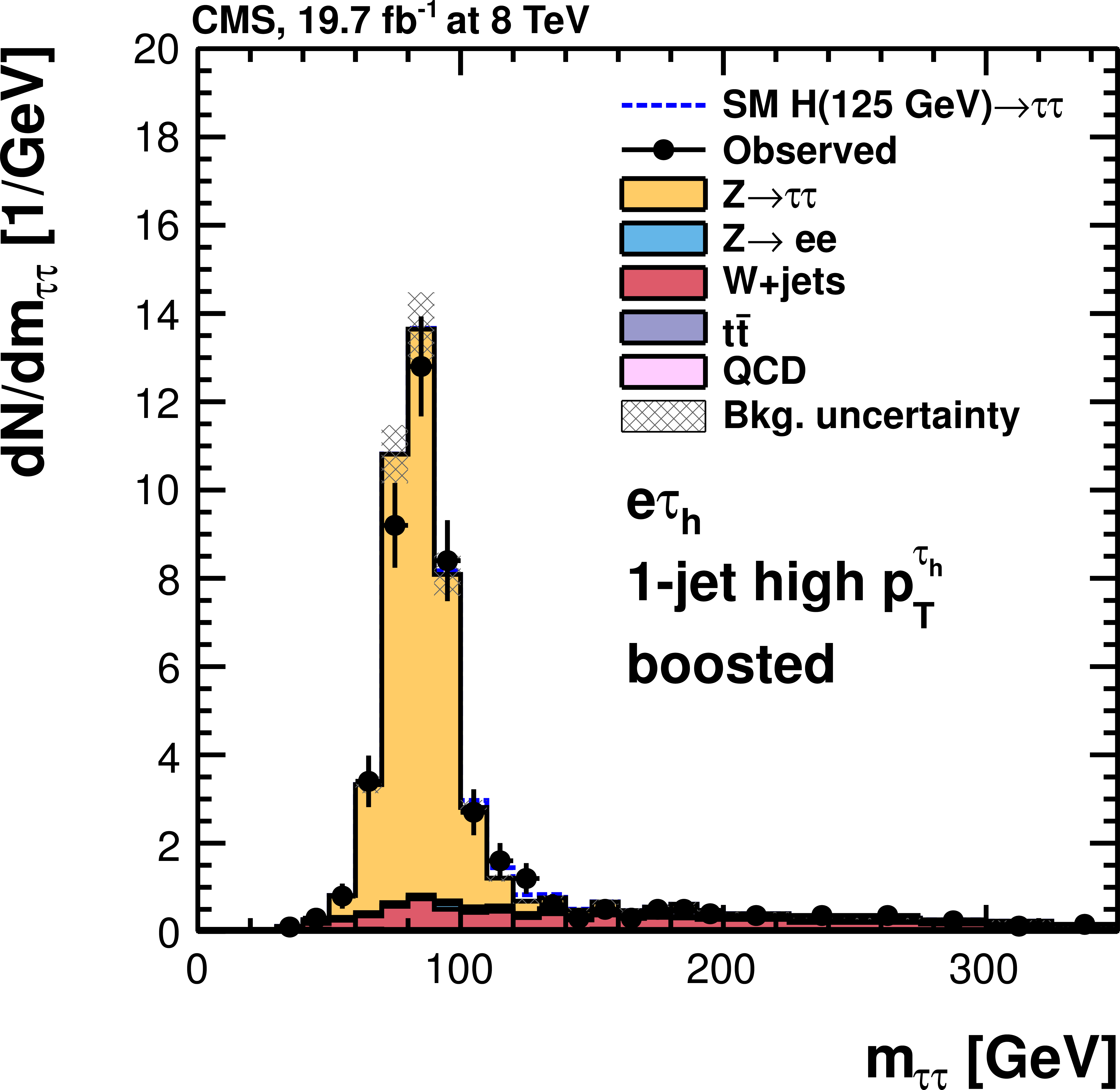
Figure 8-b:
Observed and predicted $ {m_{ {\tau } {\tau }}} $ distributions in the 8 TeV $ {{\mu }} { {\tau }_{\rm h}} $ (a, c, e) and $e { {\tau }_{\rm h}} $ (b, d, f) channels, and for the 1-jet high-$ {p_{\mathrm {T}}} ^{ { {\tau }_{\rm h}} }$ boosted (a, b), loose VBF tag (c, d), and tight VBF tag (e, f) categories. The normalization of the predicted background distributions corresponds to the result of the global fit. The signal distribution, on the other hand, is normalized to the SM prediction. The signal and background histograms are stacked. |

png pdf |
Figure 8-c:
Observed and predicted $ {m_{ {\tau } {\tau }}} $ distributions in the 8 TeV $ {{\mu }} { {\tau }_{\rm h}} $ (a, c, e) and $e { {\tau }_{\rm h}} $ (b, d, f) channels, and for the 1-jet high-$ {p_{\mathrm {T}}} ^{ { {\tau }_{\rm h}} }$ boosted (a, b), loose VBF tag (c, d), and tight VBF tag (e, f) categories. The normalization of the predicted background distributions corresponds to the result of the global fit. The signal distribution, on the other hand, is normalized to the SM prediction. The signal and background histograms are stacked. |

png pdf |
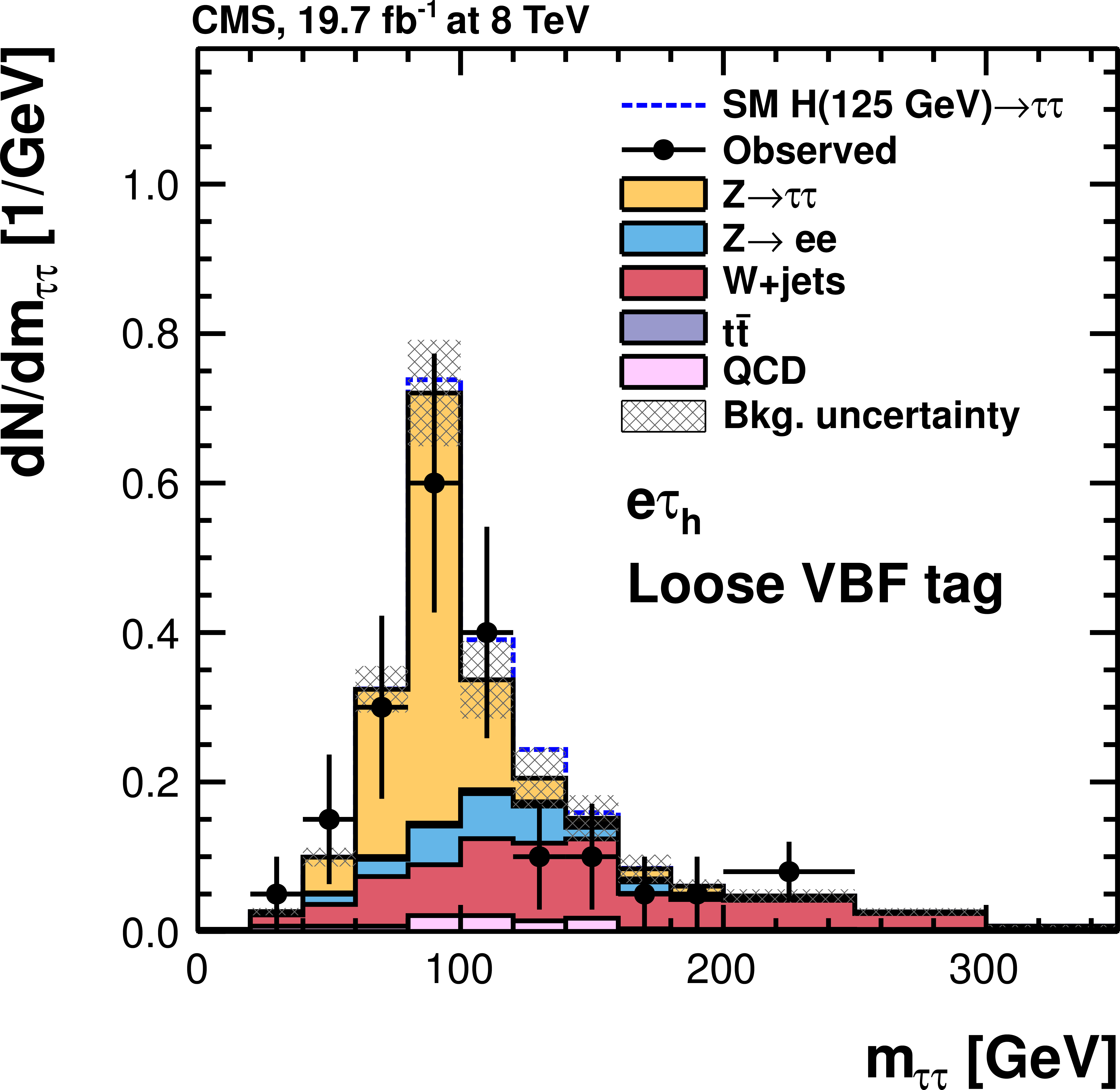
Figure 8-d:
Observed and predicted $ {m_{ {\tau } {\tau }}} $ distributions in the 8 TeV $ {{\mu }} { {\tau }_{\rm h}} $ (a, c, e) and $e { {\tau }_{\rm h}} $ (b, d, f) channels, and for the 1-jet high-$ {p_{\mathrm {T}}} ^{ { {\tau }_{\rm h}} }$ boosted (a, b), loose VBF tag (c, d), and tight VBF tag (e, f) categories. The normalization of the predicted background distributions corresponds to the result of the global fit. The signal distribution, on the other hand, is normalized to the SM prediction. The signal and background histograms are stacked. |

png pdf |
Figure 8-e:
Observed and predicted $ {m_{ {\tau } {\tau }}} $ distributions in the 8 TeV $ {{\mu }} { {\tau }_{\rm h}} $ (a, c, e) and $e { {\tau }_{\rm h}} $ (b, d, f) channels, and for the 1-jet high-$ {p_{\mathrm {T}}} ^{ { {\tau }_{\rm h}} }$ boosted (a, b), loose VBF tag (c, d), and tight VBF tag (e, f) categories. The normalization of the predicted background distributions corresponds to the result of the global fit. The signal distribution, on the other hand, is normalized to the SM prediction. The signal and background histograms are stacked. |

png pdf |
Figure 8-f:
Observed and predicted $ {m_{ {\tau } {\tau }}} $ distributions in the 8 TeV $ {{\mu }} { {\tau }_{\rm h}} $ (a, c, e) and $e { {\tau }_{\rm h}} $ (b, d, f) channels, and for the 1-jet high-$ {p_{\mathrm {T}}} ^{ { {\tau }_{\rm h}} }$ boosted (a, b), loose VBF tag (c, d), and tight VBF tag (e, f) categories. The normalization of the predicted background distributions corresponds to the result of the global fit. The signal distribution, on the other hand, is normalized to the SM prediction. The signal and background histograms are stacked. |

png pdf |
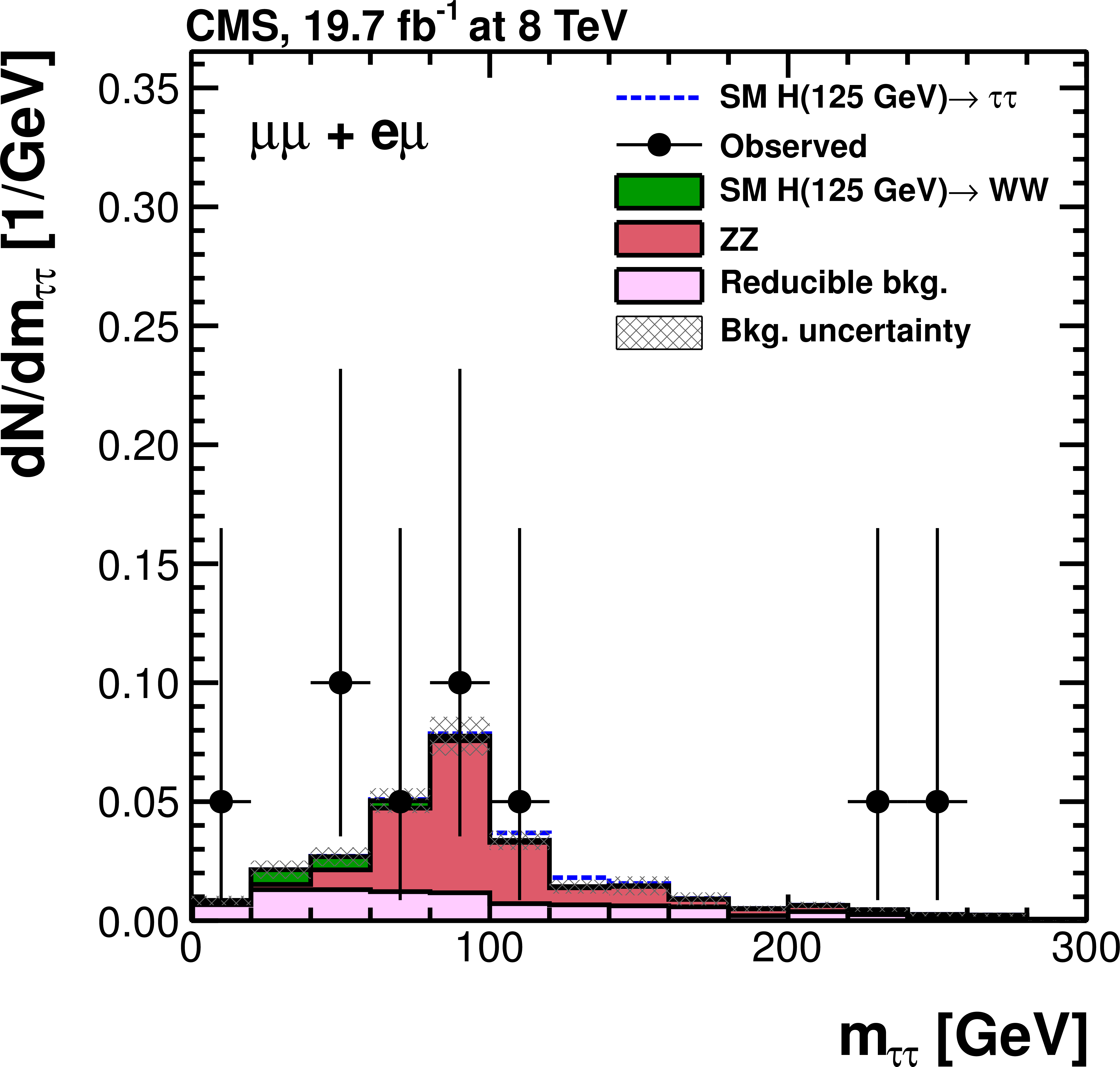
Figure 9-a:
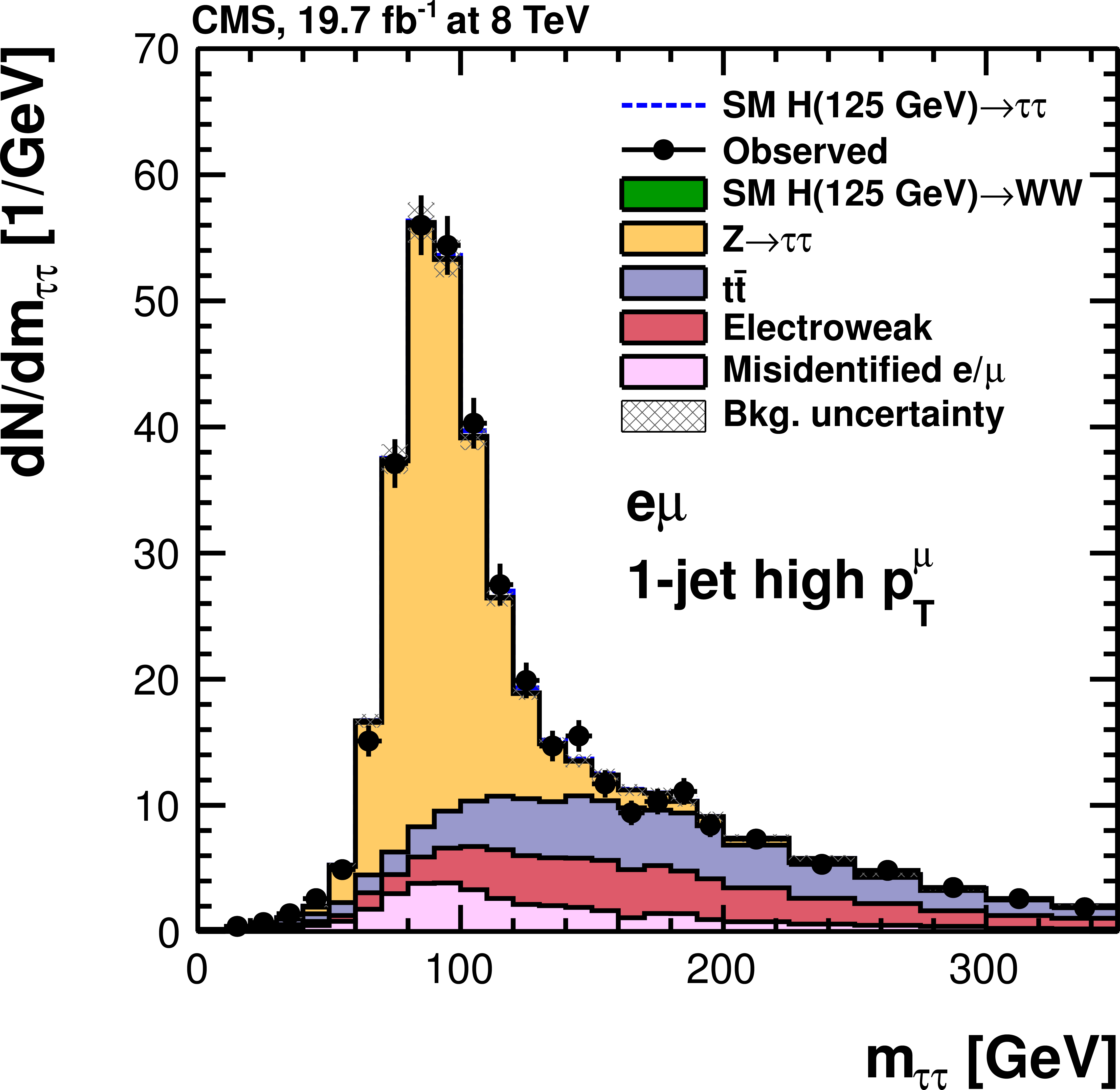
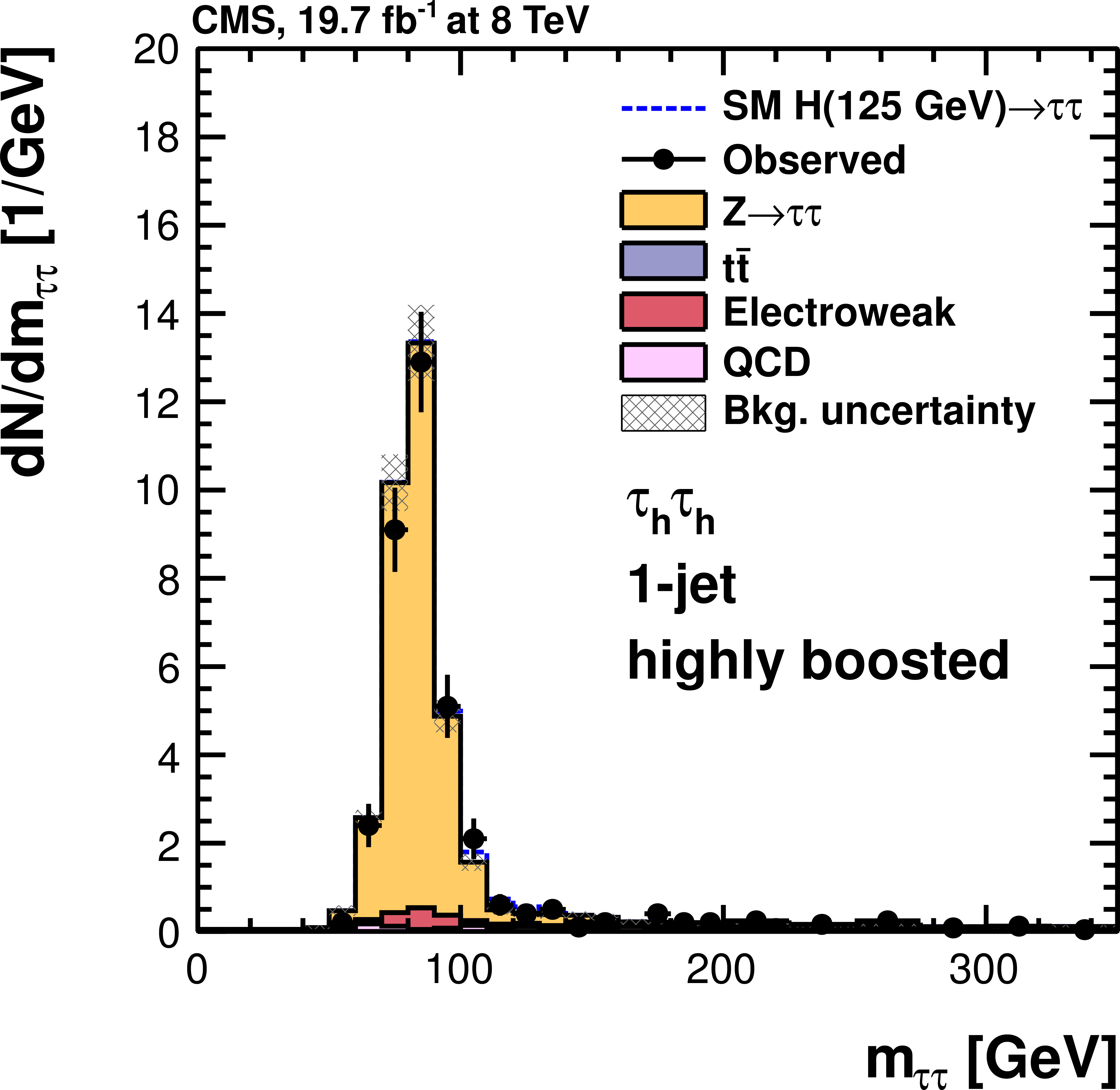
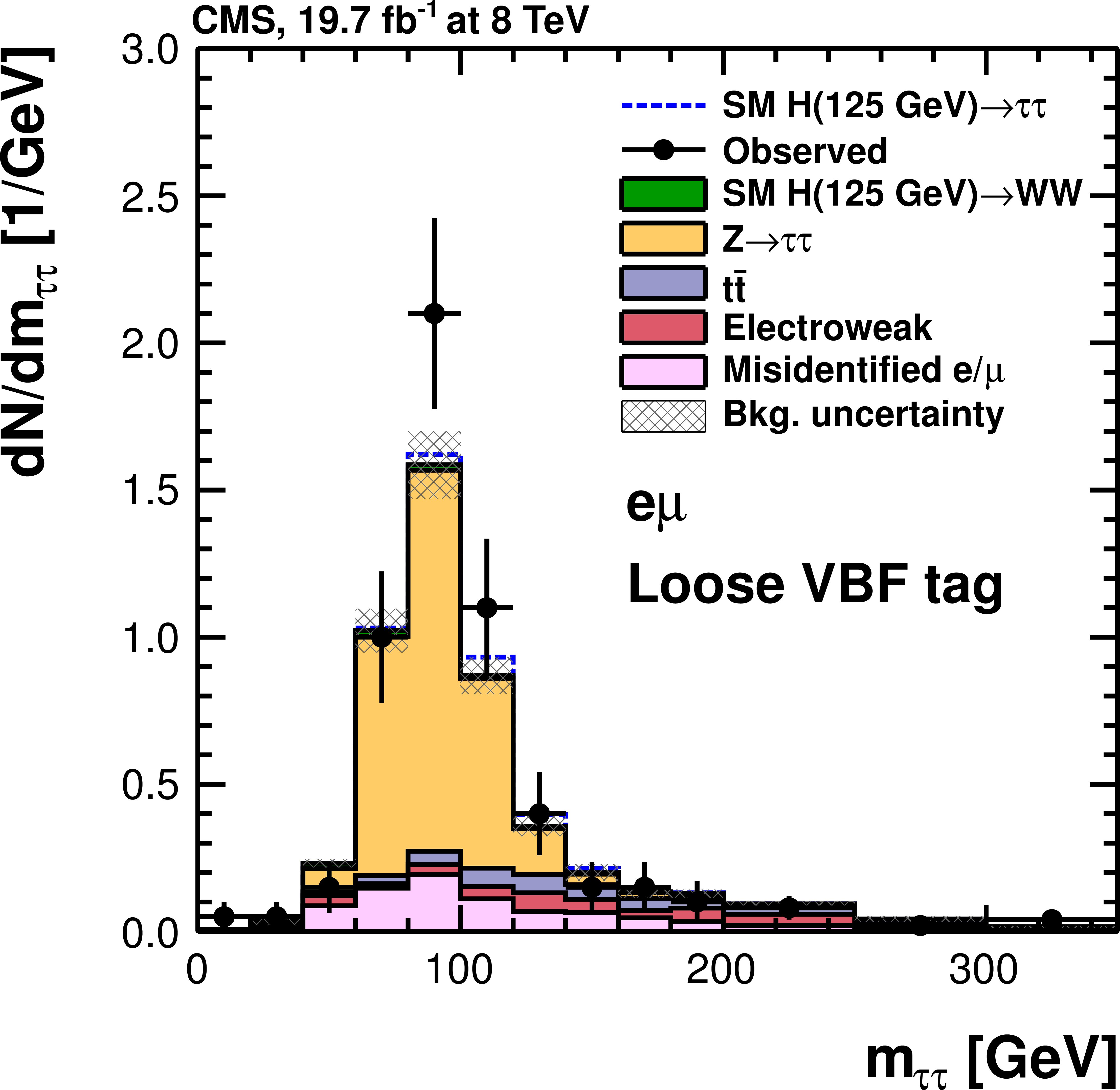
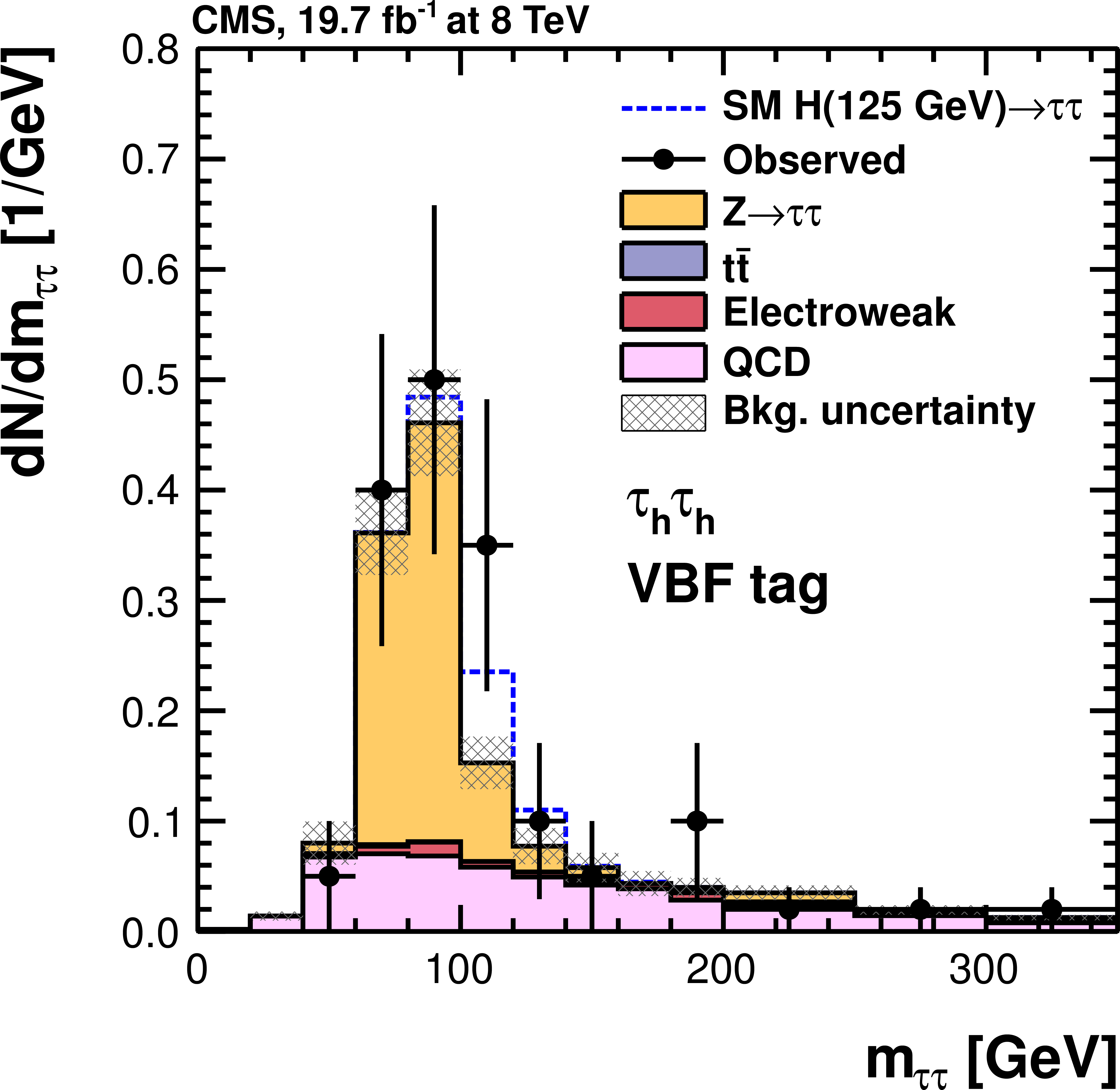
Observed and predicted $ {m_{ {\tau } {\tau }}} $ distributions in the 8 TeV $ { {\tau }_{\rm h}} { {\tau }_{\rm h}} $ (a, c, e) channel for the 1-jet boosted (a, b), 1-jet highly-boosted (c, d), and VBF-tagged (bottom) categories, and in the 8 TeV $ {\mathrm {e}} {{\mu }}$ (e, f) channel for the 1-jet high-$ {p_{\mathrm {T}}} ^ {{\mu }}$ (a, b), loose VBF tag (c, d) and tight VBF tag (e, f) categories. The normalization of the predicted background distributions corresponds to the result of the global fit. The signal distribution, on the other hand, is normalized to the SM prediction. In the $ {\mathrm {e}} {{\mu }}$ channel, the expected contribution from $ {\mathrm {H}}\to {\mathrm {W}} {\mathrm {W}}$ decays is shown separately. The signal and background histograms are stacked. |
png pdf |
Figure 9-b:
Observed and predicted $ {m_{ {\tau } {\tau }}} $ distributions in the 8 TeV $ { {\tau }_{\rm h}} { {\tau }_{\rm h}} $ (a, c, e) channel for the 1-jet boosted (a, b), 1-jet highly-boosted (c, d), and VBF-tagged (bottom) categories, and in the 8 TeV $ {\mathrm {e}} {{\mu }}$ (e, f) channel for the 1-jet high-$ {p_{\mathrm {T}}} ^ {{\mu }}$ (a, b), loose VBF tag (c, d) and tight VBF tag (e, f) categories. The normalization of the predicted background distributions corresponds to the result of the global fit. The signal distribution, on the other hand, is normalized to the SM prediction. In the $ {\mathrm {e}} {{\mu }}$ channel, the expected contribution from $ {\mathrm {H}}\to {\mathrm {W}} {\mathrm {W}}$ decays is shown separately. The signal and background histograms are stacked. |
png pdf |
Figure 9-c:
Observed and predicted $ {m_{ {\tau } {\tau }}} $ distributions in the 8 TeV $ { {\tau }_{\rm h}} { {\tau }_{\rm h}} $ (a, c, e) channel for the 1-jet boosted (a, b), 1-jet highly-boosted (c, d), and VBF-tagged (bottom) categories, and in the 8 TeV $ {\mathrm {e}} {{\mu }}$ (e, f) channel for the 1-jet high-$ {p_{\mathrm {T}}} ^ {{\mu }}$ (a, b), loose VBF tag (c, d) and tight VBF tag (e, f) categories. The normalization of the predicted background distributions corresponds to the result of the global fit. The signal distribution, on the other hand, is normalized to the SM prediction. In the $ {\mathrm {e}} {{\mu }}$ channel, the expected contribution from $ {\mathrm {H}}\to {\mathrm {W}} {\mathrm {W}}$ decays is shown separately. The signal and background histograms are stacked. |
png pdf |
Figure 9-d:
Observed and predicted $ {m_{ {\tau } {\tau }}} $ distributions in the 8 TeV $ { {\tau }_{\rm h}} { {\tau }_{\rm h}} $ (a, c, e) channel for the 1-jet boosted (a, b), 1-jet highly-boosted (c, d), and VBF-tagged (bottom) categories, and in the 8 TeV $ {\mathrm {e}} {{\mu }}$ (e, f) channel for the 1-jet high-$ {p_{\mathrm {T}}} ^ {{\mu }}$ (a, b), loose VBF tag (c, d) and tight VBF tag (e, f) categories. The normalization of the predicted background distributions corresponds to the result of the global fit. The signal distribution, on the other hand, is normalized to the SM prediction. In the $ {\mathrm {e}} {{\mu }}$ channel, the expected contribution from $ {\mathrm {H}}\to {\mathrm {W}} {\mathrm {W}}$ decays is shown separately. The signal and background histograms are stacked. |
png pdf |
Figure 9-e:
Observed and predicted $ {m_{ {\tau } {\tau }}} $ distributions in the 8 TeV $ { {\tau }_{\rm h}} { {\tau }_{\rm h}} $ (a, c, e) channel for the 1-jet boosted (a, b), 1-jet highly-boosted (c, d), and VBF-tagged (bottom) categories, and in the 8 TeV $ {\mathrm {e}} {{\mu }}$ (e, f) channel for the 1-jet high-$ {p_{\mathrm {T}}} ^ {{\mu }}$ (a, b), loose VBF tag (c, d) and tight VBF tag (e, f) categories. The normalization of the predicted background distributions corresponds to the result of the global fit. The signal distribution, on the other hand, is normalized to the SM prediction. In the $ {\mathrm {e}} {{\mu }}$ channel, the expected contribution from $ {\mathrm {H}}\to {\mathrm {W}} {\mathrm {W}}$ decays is shown separately. The signal and background histograms are stacked. |

png pdf |
Figure 9-f:
Observed and predicted $ {m_{ {\tau } {\tau }}} $ distributions in the 8 TeV $ { {\tau }_{\rm h}} { {\tau }_{\rm h}} $ (a, c, e) channel for the 1-jet boosted (a, b), 1-jet highly-boosted (c, d), and VBF-tagged (bottom) categories, and in the 8 TeV $ {\mathrm {e}} {{\mu }}$ (e, f) channel for the 1-jet high-$ {p_{\mathrm {T}}} ^ {{\mu }}$ (a, b), loose VBF tag (c, d) and tight VBF tag (e, f) categories. The normalization of the predicted background distributions corresponds to the result of the global fit. The signal distribution, on the other hand, is normalized to the SM prediction. In the $ {\mathrm {e}} {{\mu }}$ channel, the expected contribution from $ {\mathrm {H}}\to {\mathrm {W}} {\mathrm {W}}$ decays is shown separately. The signal and background histograms are stacked. |
png pdf |
Figure 10-a:
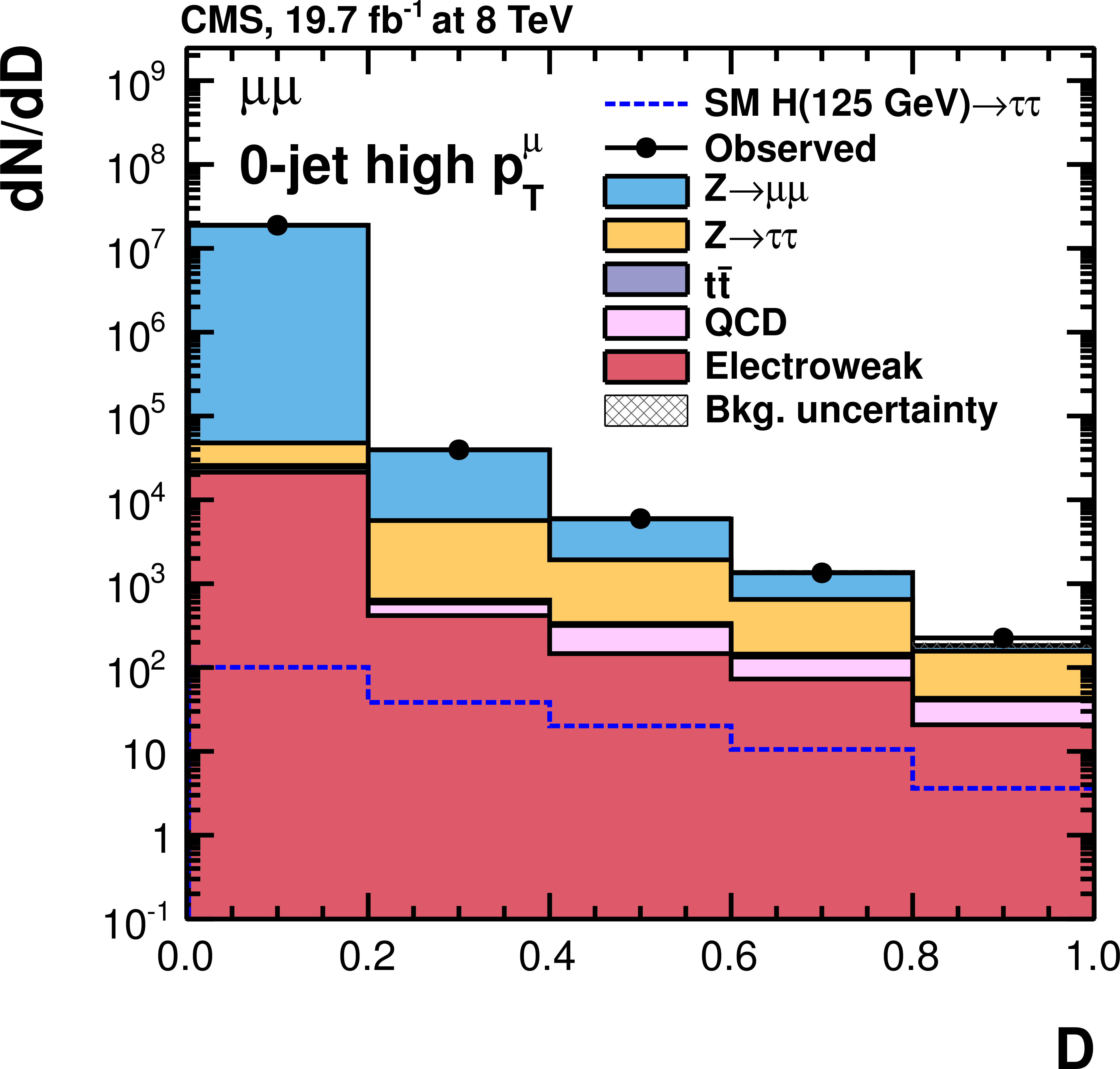
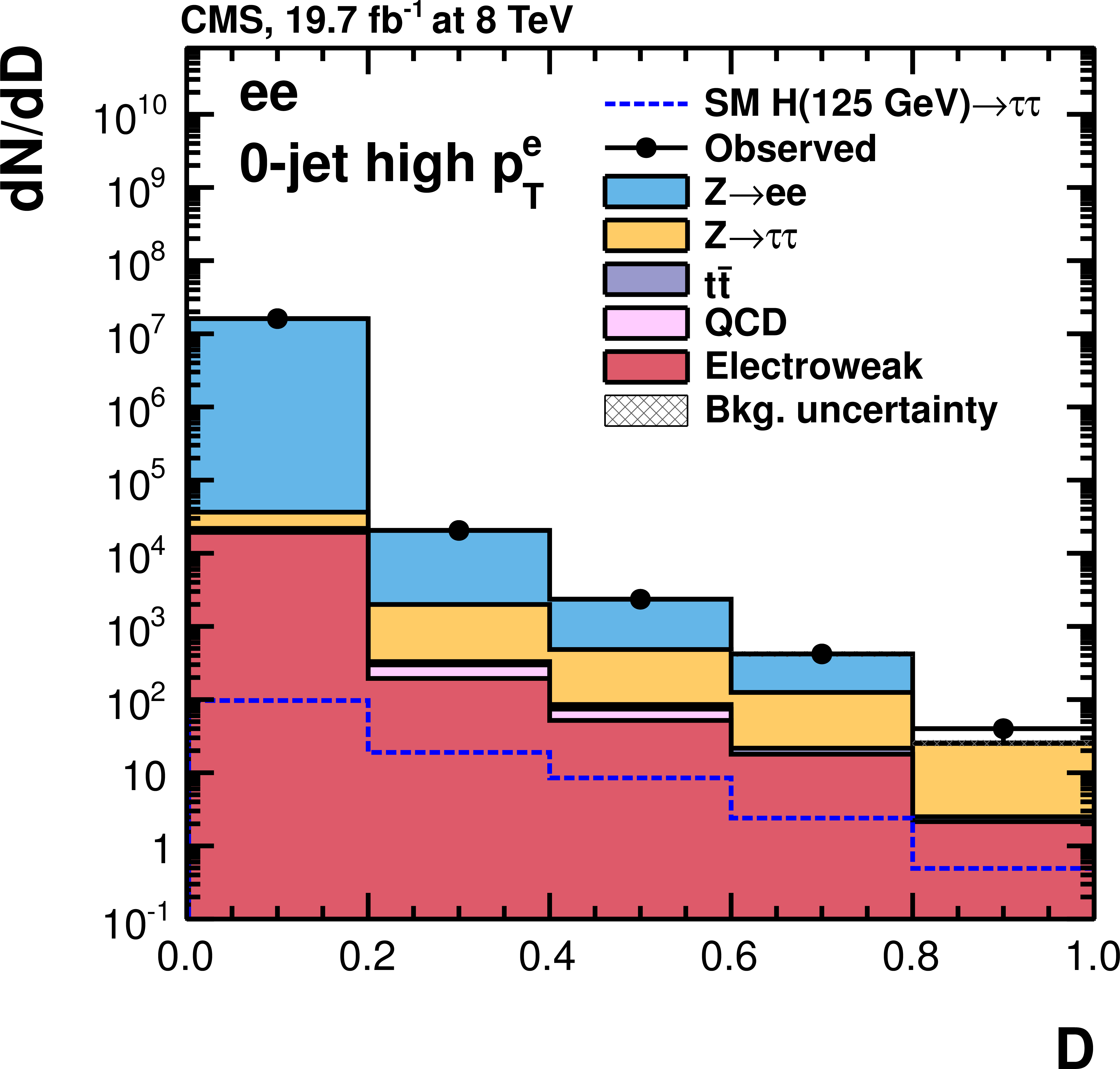
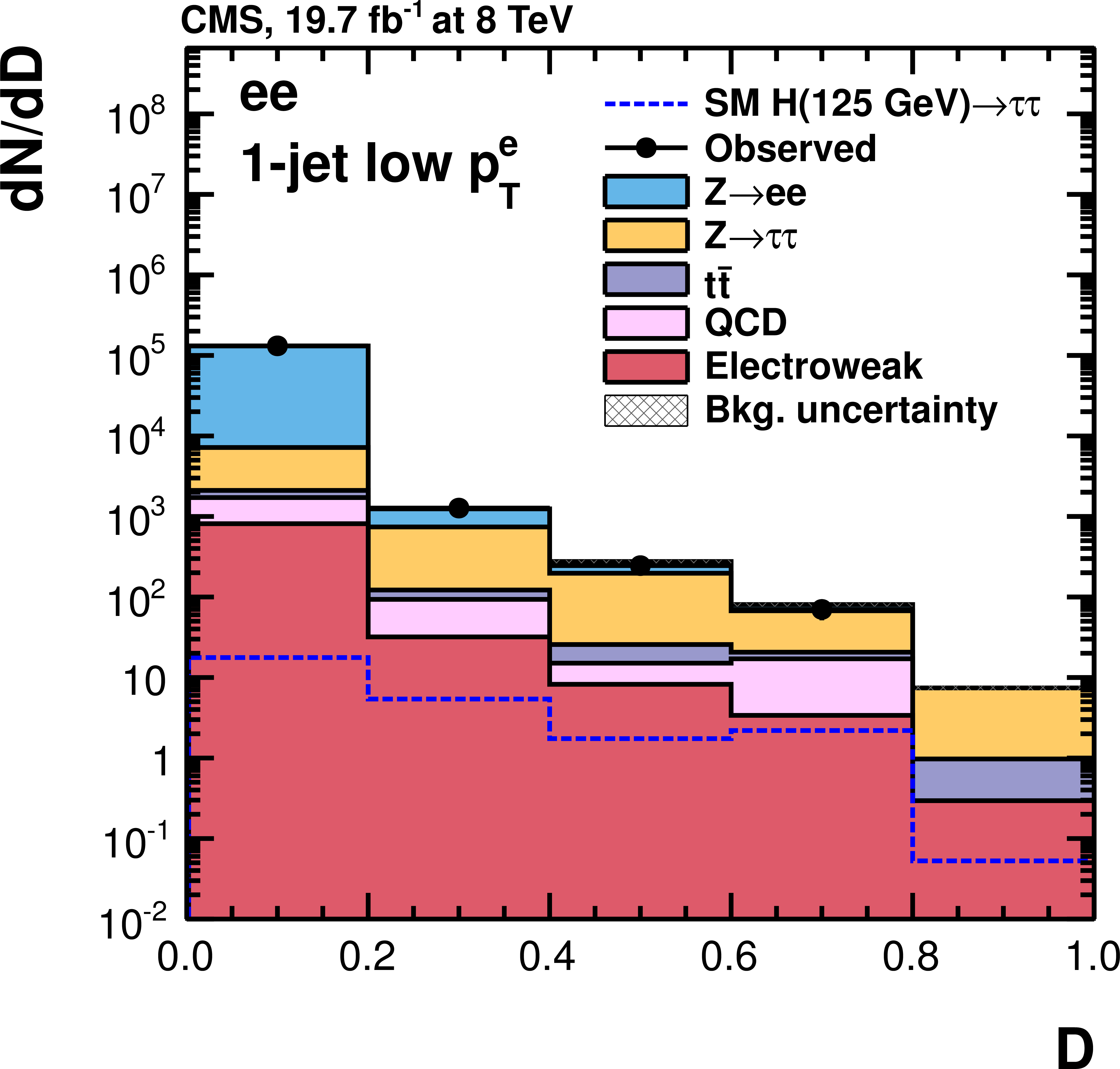
Observed and predicted distributions for the final discriminator $D$ in the 8 TeV $ {{\mu }} {{\mu }}$ (a, c, e) and $ {\mathrm {e}} {\mathrm {e}}$ (b, d, f) channels, and for the 0-jet high-$ {p_{\mathrm {T}}} ^\ell $ (a, b), 1-jet high-$ {p_{\mathrm {T}}} ^\ell $ (c, d), and 2-jet (e, f) categories. The normalization of the predicted background distributions corresponds to the result of the global fit. The signal distribution, on the other hand, is normalized to the SM prediction. The open signal histogram is shown superimposed to the background histograms, which are stacked. |
png pdf |
Figure 10-b:
Observed and predicted distributions for the final discriminator $D$ in the 8 TeV $ {{\mu }} {{\mu }}$ (a, c, e) and $ {\mathrm {e}} {\mathrm {e}}$ (b, d, f) channels, and for the 0-jet high-$ {p_{\mathrm {T}}} ^\ell $ (a, b), 1-jet high-$ {p_{\mathrm {T}}} ^\ell $ (c, d), and 2-jet (e, f) categories. The normalization of the predicted background distributions corresponds to the result of the global fit. The signal distribution, on the other hand, is normalized to the SM prediction. The open signal histogram is shown superimposed to the background histograms, which are stacked. |

png pdf |
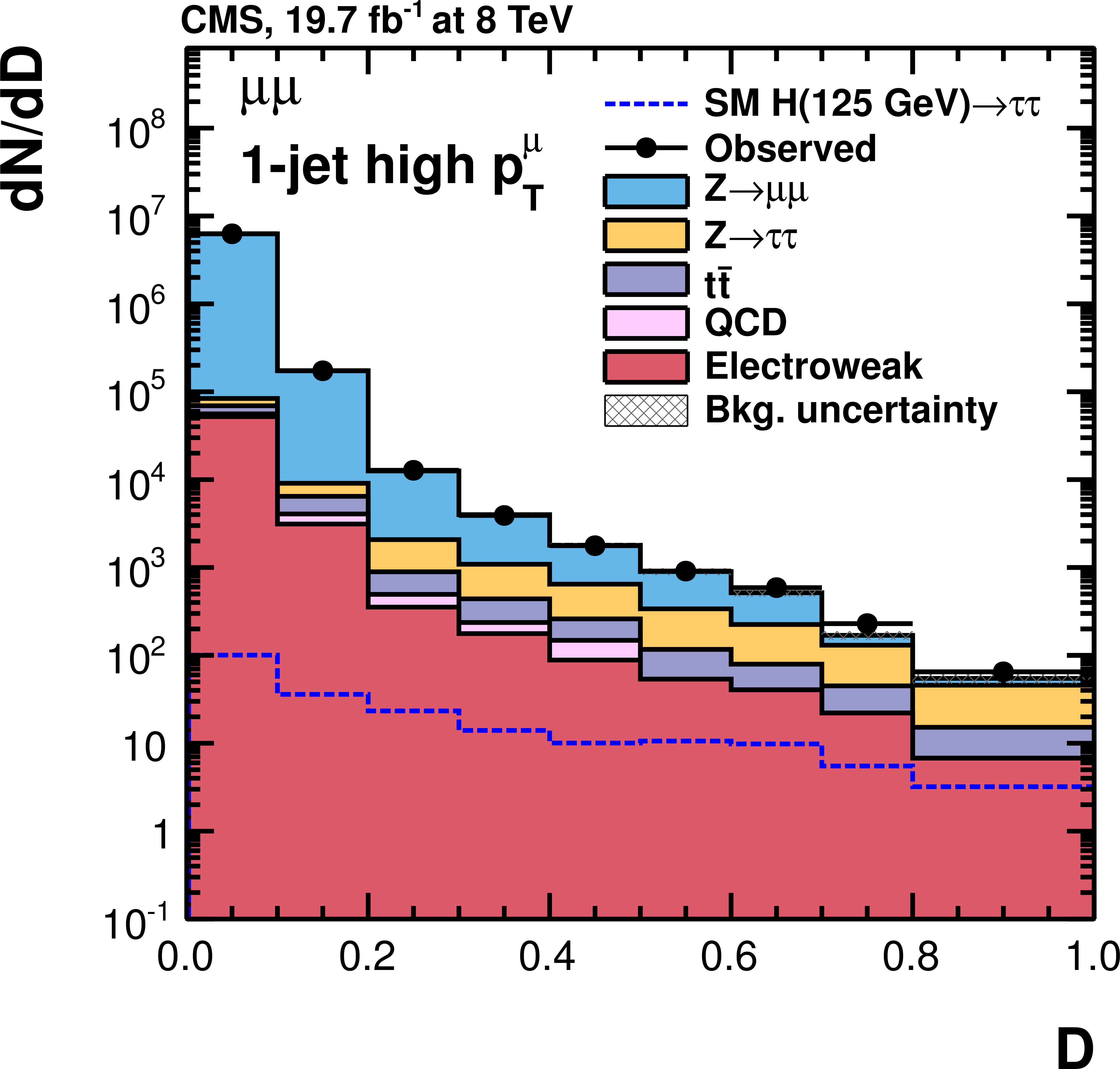
Figure 10-c:
Observed and predicted distributions for the final discriminator $D$ in the 8 TeV $ {{\mu }} {{\mu }}$ (a, c, e) and $ {\mathrm {e}} {\mathrm {e}}$ (b, d, f) channels, and for the 0-jet high-$ {p_{\mathrm {T}}} ^\ell $ (a, b), 1-jet high-$ {p_{\mathrm {T}}} ^\ell $ (c, d), and 2-jet (e, f) categories. The normalization of the predicted background distributions corresponds to the result of the global fit. The signal distribution, on the other hand, is normalized to the SM prediction. The open signal histogram is shown superimposed to the background histograms, which are stacked. |

png pdf |
Figure 10-d:
Observed and predicted distributions for the final discriminator $D$ in the 8 TeV $ {{\mu }} {{\mu }}$ (a, c, e) and $ {\mathrm {e}} {\mathrm {e}}$ (b, d, f) channels, and for the 0-jet high-$ {p_{\mathrm {T}}} ^\ell $ (a, b), 1-jet high-$ {p_{\mathrm {T}}} ^\ell $ (c, d), and 2-jet (e, f) categories. The normalization of the predicted background distributions corresponds to the result of the global fit. The signal distribution, on the other hand, is normalized to the SM prediction. The open signal histogram is shown superimposed to the background histograms, which are stacked. |
png pdf |
Figure 10-e:
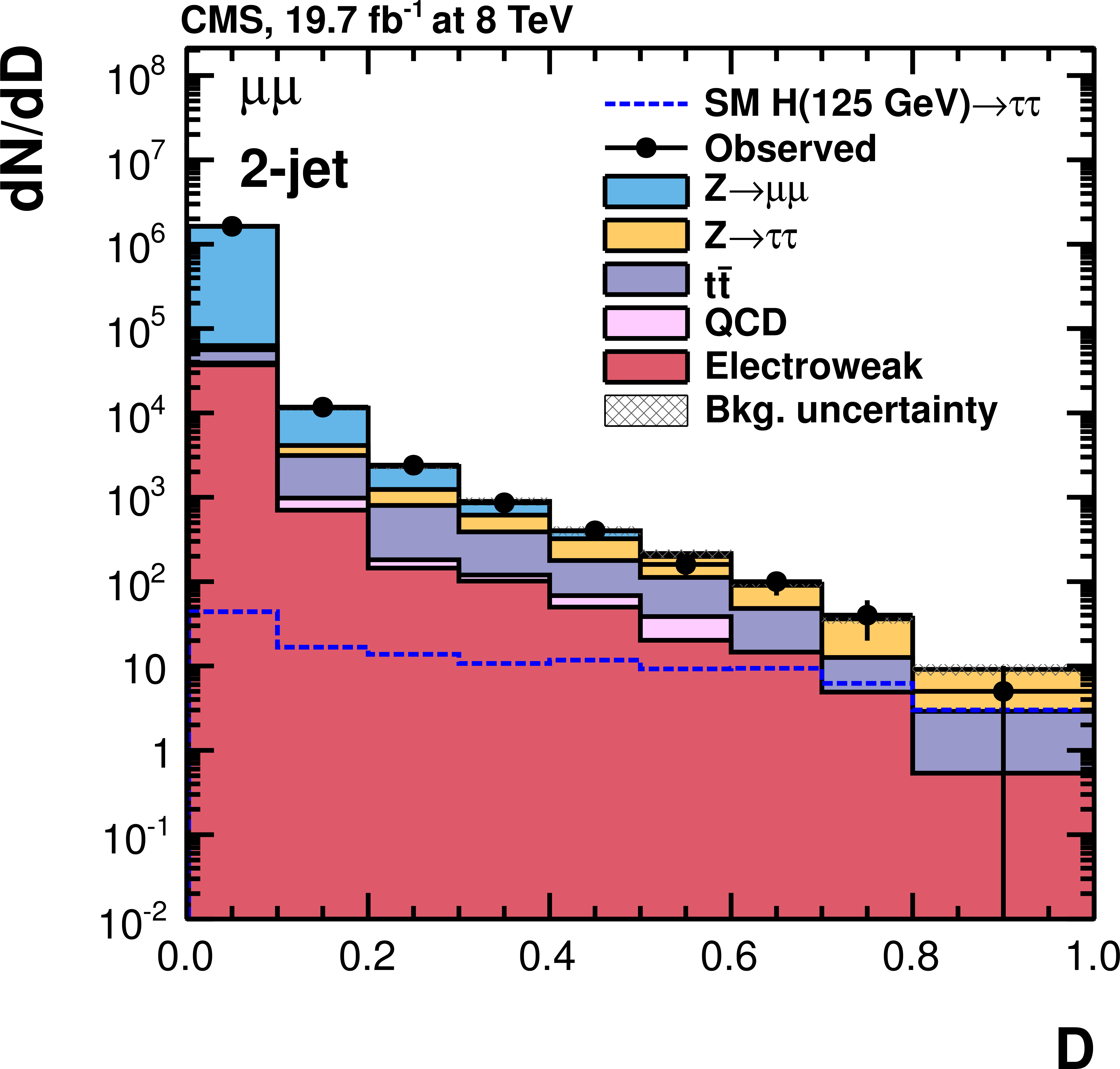
Observed and predicted distributions for the final discriminator $D$ in the 8 TeV $ {{\mu }} {{\mu }}$ (a, c, e) and $ {\mathrm {e}} {\mathrm {e}}$ (b, d, f) channels, and for the 0-jet high-$ {p_{\mathrm {T}}} ^\ell $ (a, b), 1-jet high-$ {p_{\mathrm {T}}} ^\ell $ (c, d), and 2-jet (e, f) categories. The normalization of the predicted background distributions corresponds to the result of the global fit. The signal distribution, on the other hand, is normalized to the SM prediction. The open signal histogram is shown superimposed to the background histograms, which are stacked. |

png pdf |
Figure 10-f:
Observed and predicted distributions for the final discriminator $D$ in the 8 TeV $ {{\mu }} {{\mu }}$ (a, c, e) and $ {\mathrm {e}} {\mathrm {e}}$ (b, d, f) channels, and for the 0-jet high-$ {p_{\mathrm {T}}} ^\ell $ (a, b), 1-jet high-$ {p_{\mathrm {T}}} ^\ell $ (c, d), and 2-jet (e, f) categories. The normalization of the predicted background distributions corresponds to the result of the global fit. The signal distribution, on the other hand, is normalized to the SM prediction. The open signal histogram is shown superimposed to the background histograms, which are stacked. |
png pdf |
Figure 11:
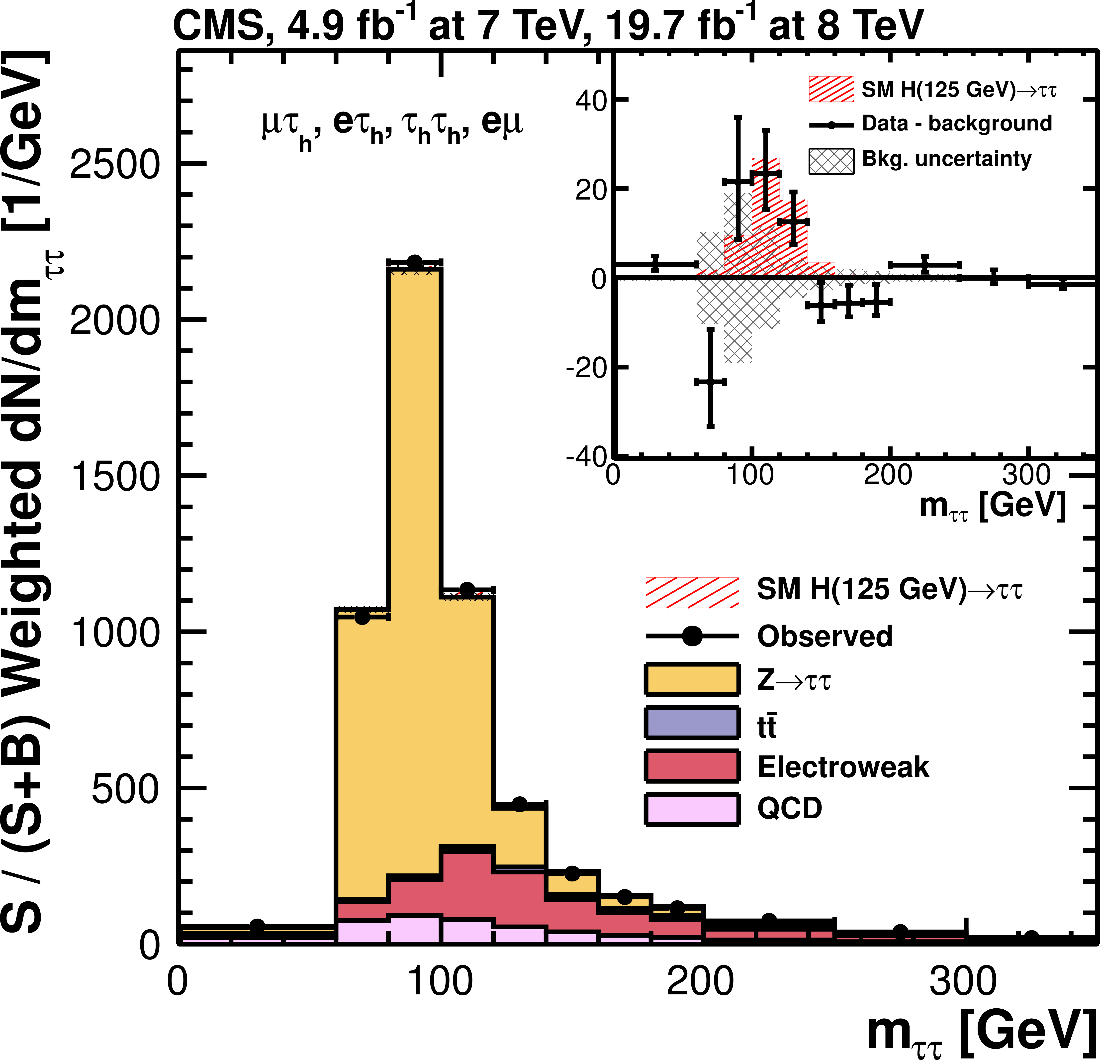
Combined observed and predicted $ {m_{ {\tau } {\tau }}} $ distributions for the $ {{\mu }} { {\tau }_{\rm h}} $, $ {\mathrm {e}} { {\tau }_{\rm h}} $, $ { {\tau }_{\rm h}} { {\tau }_{\rm h}} $, and $ {\mathrm {e}} {{\mu }}$ channels. The normalization of the predicted background distributions corresponds to the result of the global fit. The signal distribution, on the other hand, is normalized to the SM prediction ($\mu = 1$). The distributions obtained in each category of each channel are weighted by the ratio between the expected signal and signal-plus-background yields in the category, obtained in the central $ {m_{ {\tau } {\tau }}} $ interval containing 68% of the signal events. The inset shows the corresponding difference between the observed data and expected background distributions, together with the signal distribution for a SM Higgs boson at $ {m_{ {\mathrm {H}} }}$ = 125 GeV. The distribution from SM Higgs boson events in the $ {\mathrm {W}} {\mathrm {W}}$ decay channel does not significantly contribute to this plot. |
png pdf |
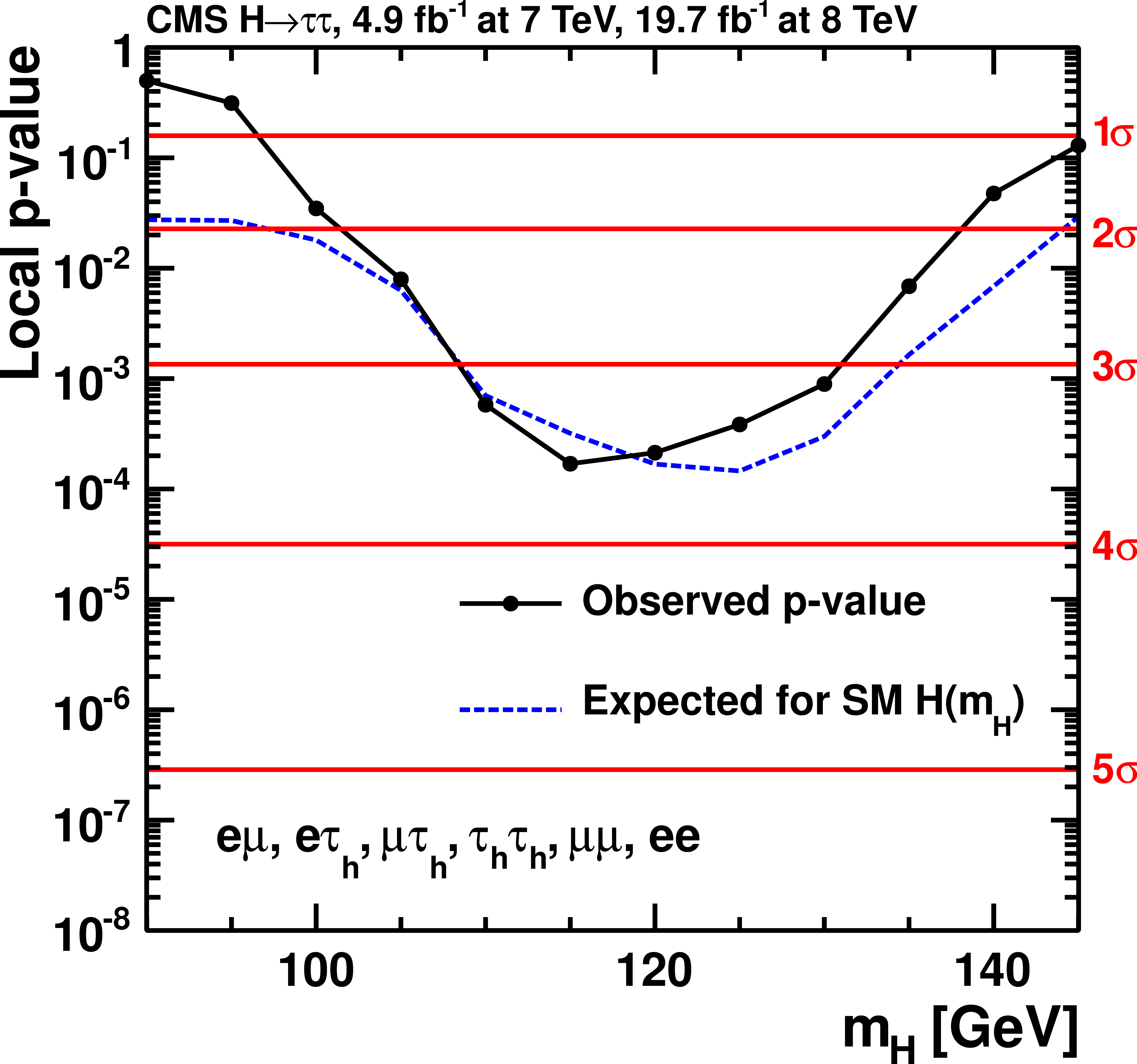
Figure 12:
Local $p$-value and significance in number of standard deviations as a function of the SM Higgs boson mass hypothesis for the $LL'$ channels. The observation (solid line) is compared to the expectation (dashed line) for a SM Higgs boson with mass $ {m_{ {\mathrm {H}} }} $. The background-only hypothesis includes the $ {\mathrm {p}} {\mathrm {p}}\to {\mathrm {H}} \text {(125 GeV)}\to {\mathrm {W}} {\mathrm {W}}$ process for every value of $ {m_{ {\mathrm {H}} }} $. |
png pdf |
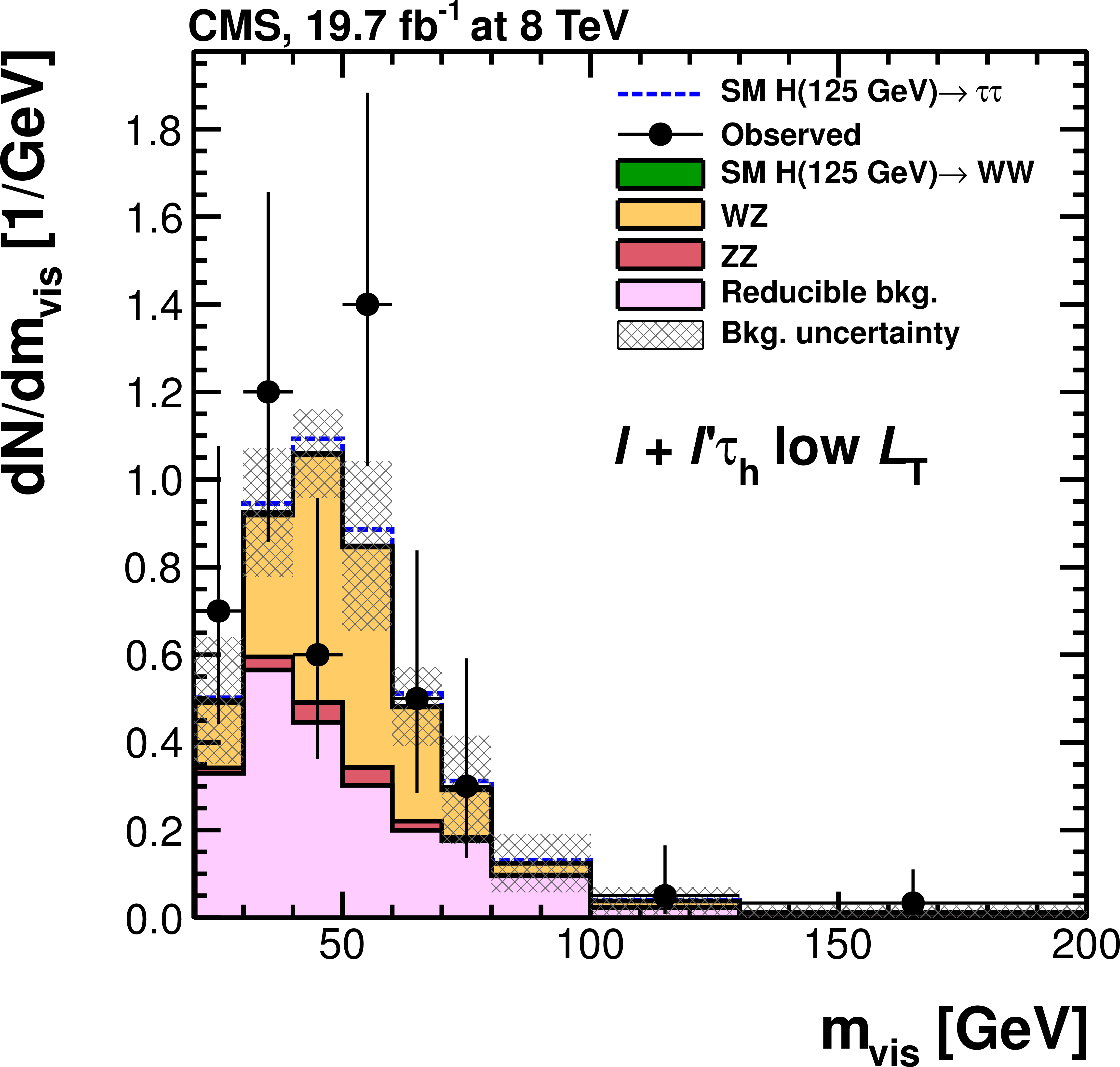
Figure 13-a:
Observed and predicted $ {m_\text {vis}} $ distributions in the $\ell +\ell ' { {\tau }_{\rm h}} $ channel in the low-$ {L_\mathrm {T}} $ (a) and high-$ {L_\mathrm {T}} $ (b) categories, each for the 8 TeV dataset, and in the $\ell + { {\tau }_{\rm h}} { {\tau }_{\rm h}} $ channel (c); observed and predicted $ {m_{ {\tau } {\tau }}} $ distributions in the $\ell \ell + LL'$ channel (d). The normalization of the predicted background distributions corresponds to the result of the global fit. The signal distribution, on the other hand, is normalized to the SM prediction ($\mu = 1$). The signal and background histograms are stacked. |
png pdf |
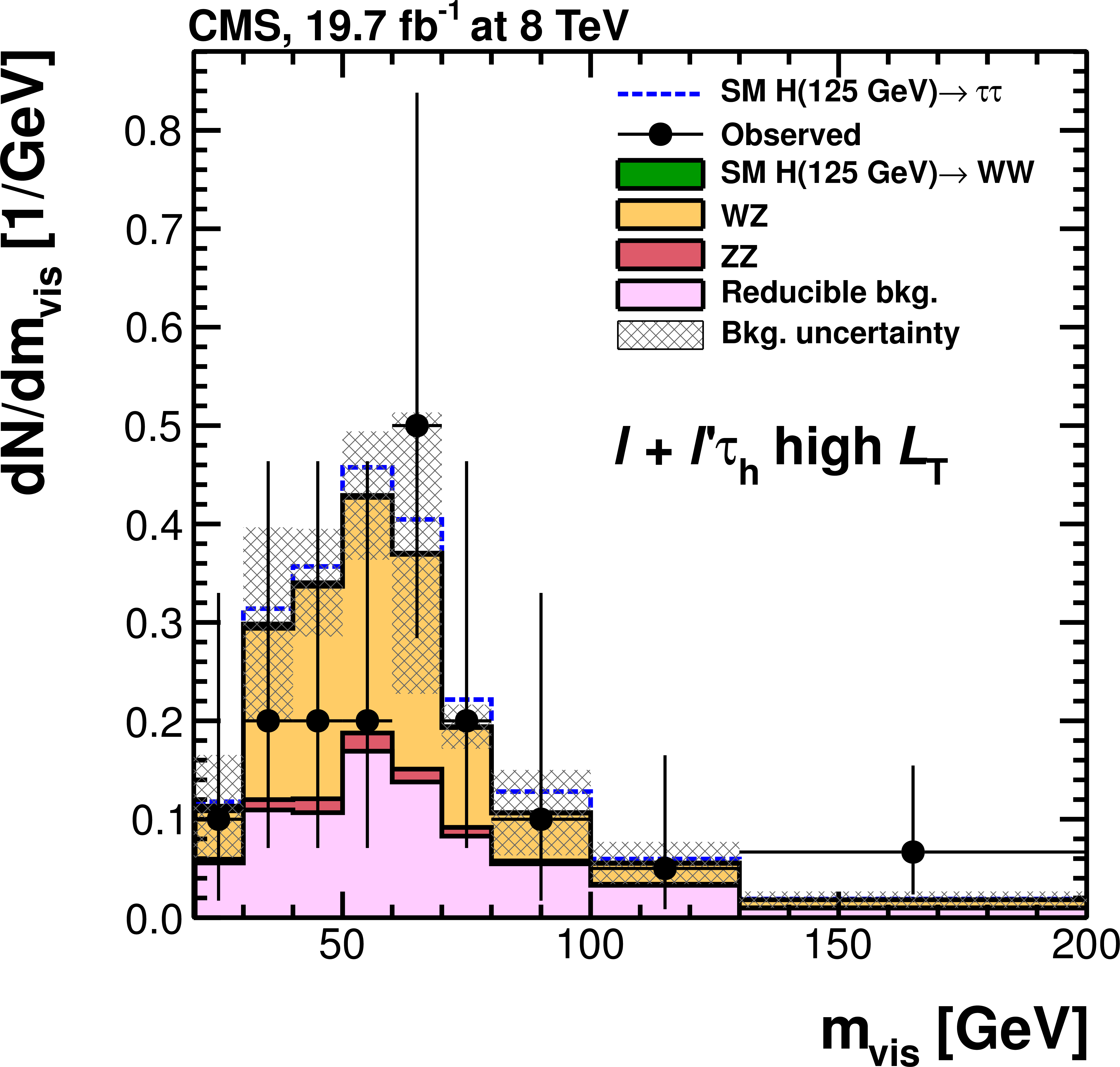
Figure 13-b:
Observed and predicted $ {m_\text {vis}} $ distributions in the $\ell +\ell ' { {\tau }_{\rm h}} $ channel in the low-$ {L_\mathrm {T}} $ (a) and high-$ {L_\mathrm {T}} $ (b) categories, each for the 8 TeV dataset, and in the $\ell + { {\tau }_{\rm h}} { {\tau }_{\rm h}} $ channel (c); observed and predicted $ {m_{ {\tau } {\tau }}} $ distributions in the $\ell \ell + LL'$ channel (d). The normalization of the predicted background distributions corresponds to the result of the global fit. The signal distribution, on the other hand, is normalized to the SM prediction ($\mu = 1$). The signal and background histograms are stacked. |
png pdf |
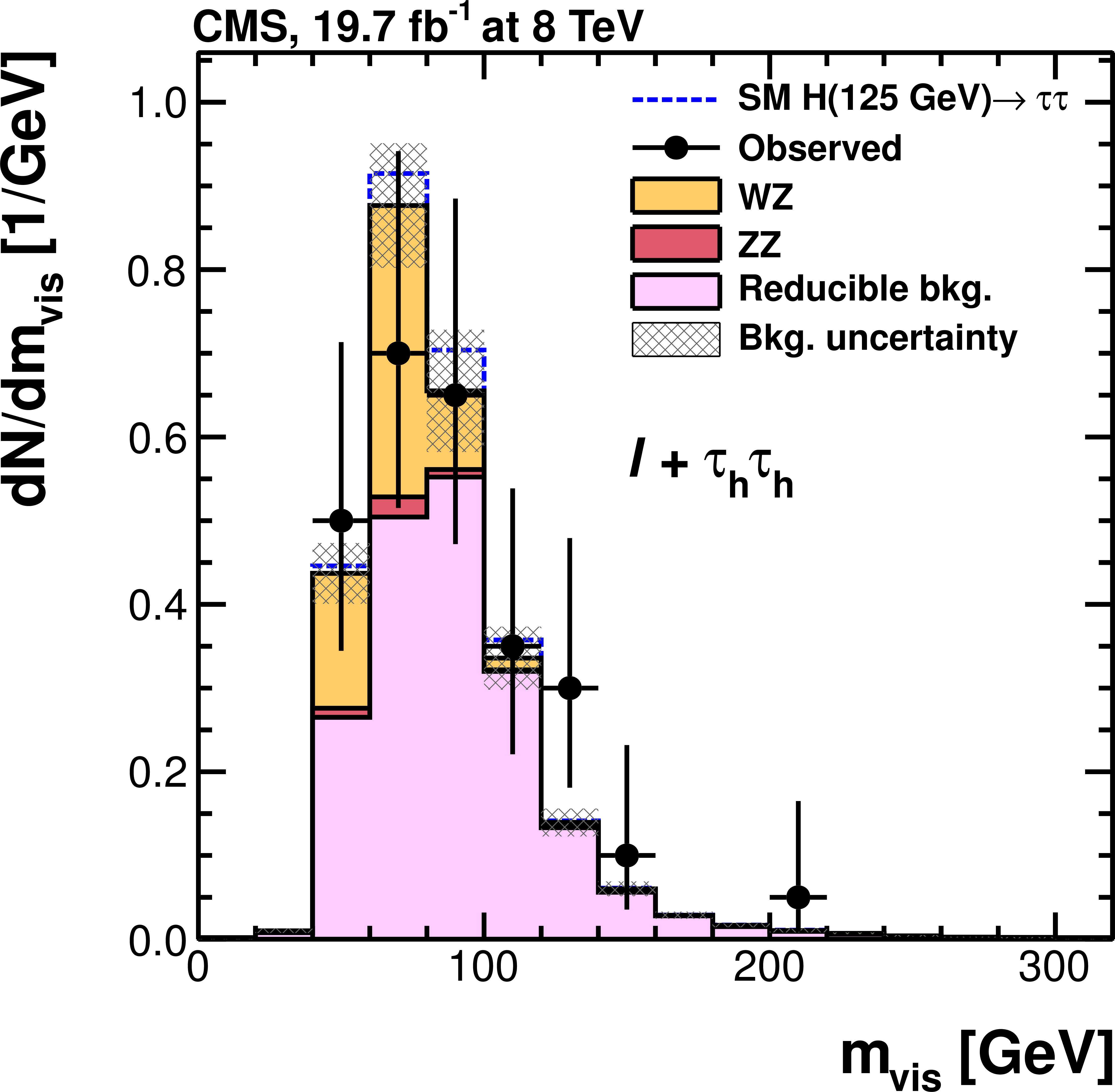
Figure 13-c:
Observed and predicted $ {m_\text {vis}} $ distributions in the $\ell +\ell ' { {\tau }_{\rm h}} $ channel in the low-$ {L_\mathrm {T}} $ (a) and high-$ {L_\mathrm {T}} $ (b) categories, each for the 8 TeV dataset, and in the $\ell + { {\tau }_{\rm h}} { {\tau }_{\rm h}} $ channel (c); observed and predicted $ {m_{ {\tau } {\tau }}} $ distributions in the $\ell \ell + LL'$ channel (d). The normalization of the predicted background distributions corresponds to the result of the global fit. The signal distribution, on the other hand, is normalized to the SM prediction ($\mu = 1$). The signal and background histograms are stacked. |
png pdf |
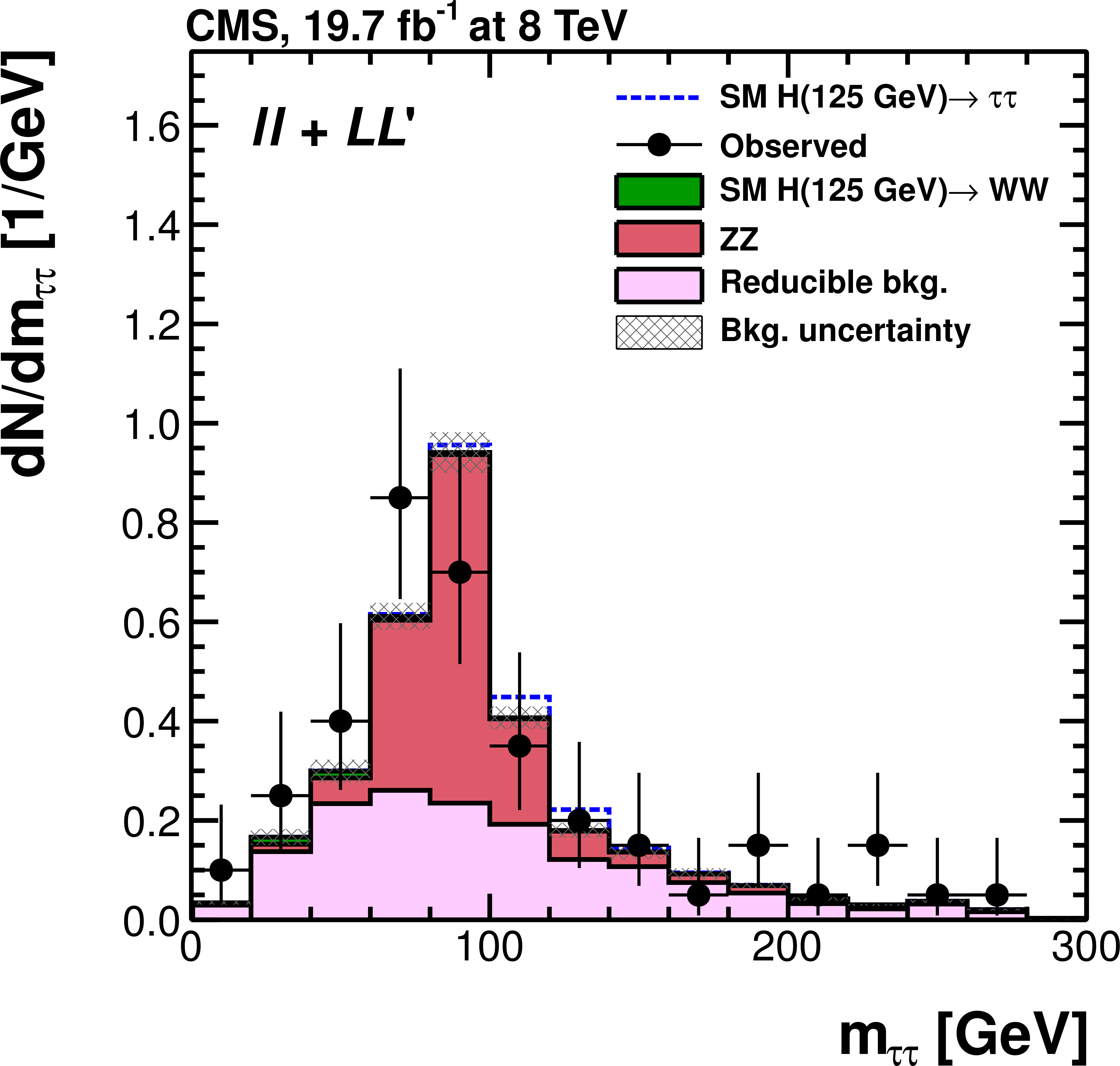
Figure 13-d:
Observed and predicted $ {m_\text {vis}} $ distributions in the $\ell +\ell ' { {\tau }_{\rm h}} $ channel in the low-$ {L_\mathrm {T}} $ (a) and high-$ {L_\mathrm {T}} $ (b) categories, each for the 8 TeV dataset, and in the $\ell + { {\tau }_{\rm h}} { {\tau }_{\rm h}} $ channel (c); observed and predicted $ {m_{ {\tau } {\tau }}} $ distributions in the $\ell \ell + LL'$ channel (d). The normalization of the predicted background distributions corresponds to the result of the global fit. The signal distribution, on the other hand, is normalized to the SM prediction ($\mu = 1$). The signal and background histograms are stacked. |

png pdf |
Figure 14-a:
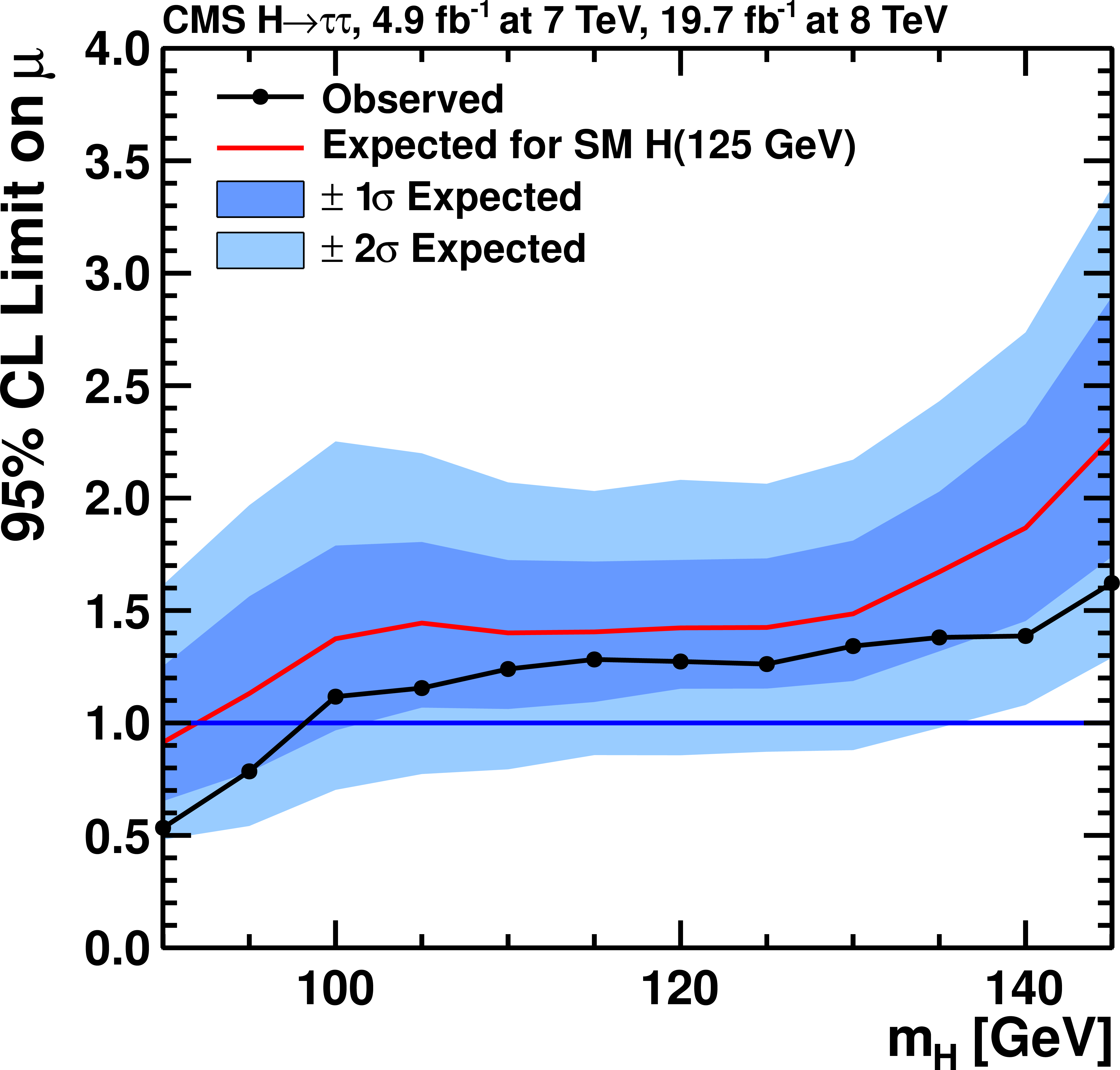
Combined observed 95% CL upper limit on the signal strength parameter $\mu $, together with the expected limit obtained in the background-only hypothesis (a), and the signal-plus-background hypothesis for a SM Higgs boson with $ {m_{ {\mathrm {H}} }}$ = 125 GeV (b). The background-only hypothesis includes the $ {\mathrm {p}} {\mathrm {p}}\rightarrow {\mathrm {H}} \text {(125 GeV)}\to {\mathrm {W}} {\mathrm {W}}$ process for every value of $ {m_{ {\mathrm {H}} }} $. The bands show the expected one- and two-standard-deviation probability intervals around the expected limit. |
png pdf |
Figure 14-b:
Combined observed 95% CL upper limit on the signal strength parameter $\mu $, together with the expected limit obtained in the background-only hypothesis (a), and the signal-plus-background hypothesis for a SM Higgs boson with $ {m_{ {\mathrm {H}} }}$ = 125 GeV (b). The background-only hypothesis includes the $ {\mathrm {p}} {\mathrm {p}}\rightarrow {\mathrm {H}} \text {(125 GeV)}\to {\mathrm {W}} {\mathrm {W}}$ process for every value of $ {m_{ {\mathrm {H}} }} $. The bands show the expected one- and two-standard-deviation probability intervals around the expected limit. |
png pdf |
Figure 15:
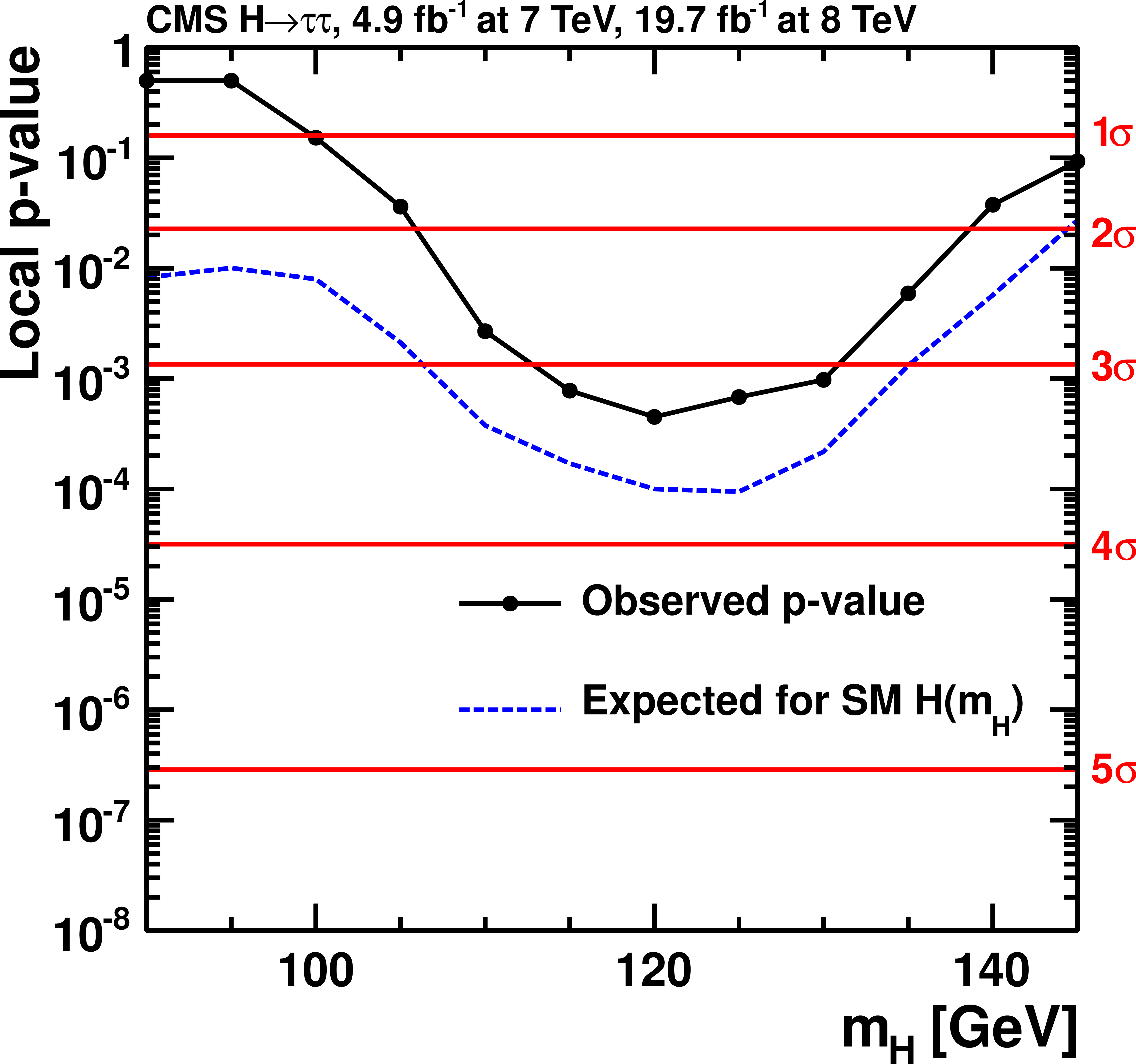
Local $p$-value and significance in number of standard deviations as a function of the SM Higgs boson mass hypothesis for the combination of all decay channels. The observation (solid line) is compared to the expectation (dashed line) for a SM Higgs boson with mass $ {m_{ {\mathrm {H}} }} $. The background-only hypothesis includes the $ {\mathrm {p}} {\mathrm {p}}\to {\mathrm {H}} \text {(125 GeV)}\to {\mathrm {W}} {\mathrm {W}}$ process for every value of $ {m_{ {\mathrm {H}} }} $. |

png pdf |
Figure 16-a:
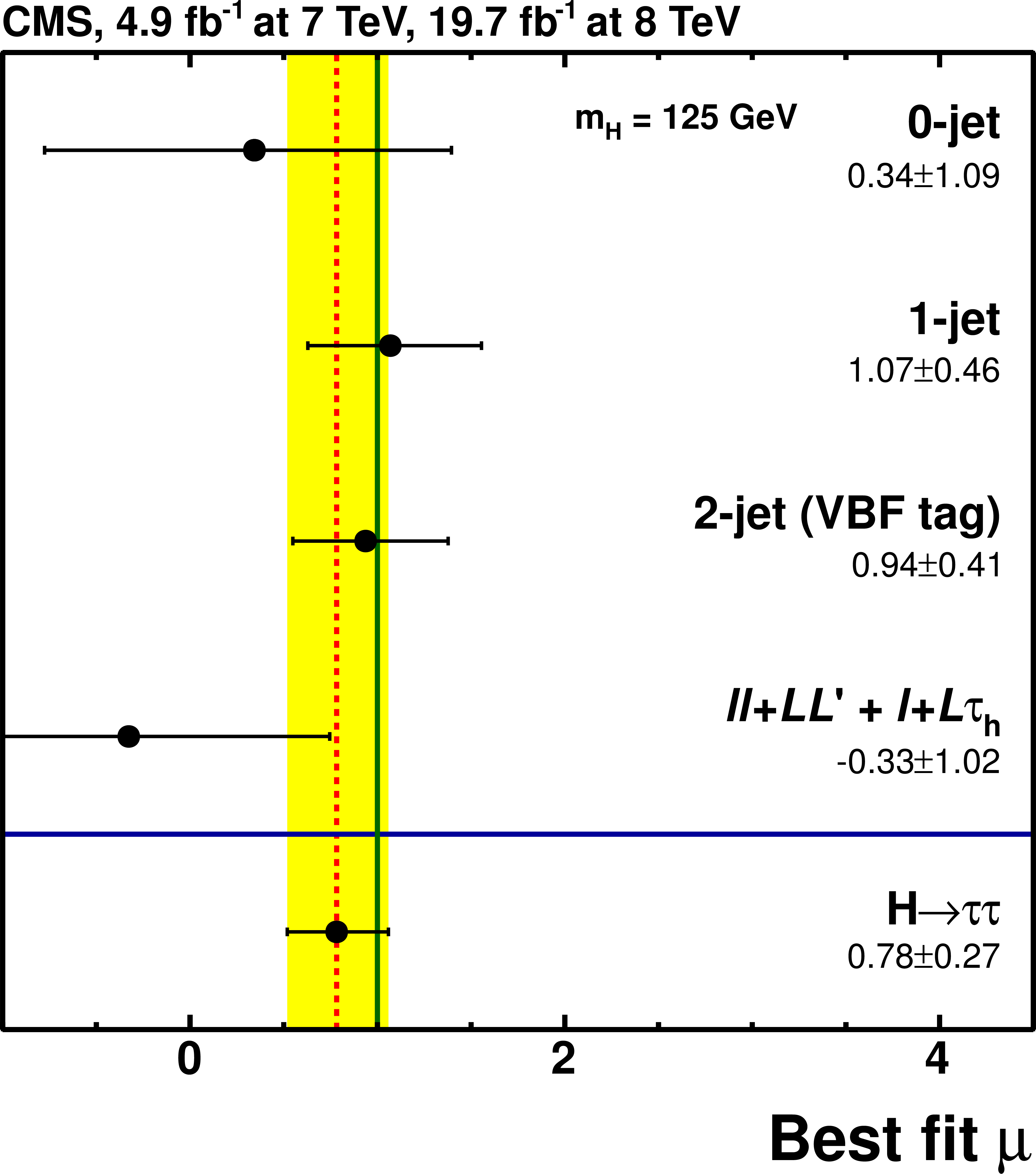
Best-fit signal strength values, for independent channels (a) and categories (b), for $ {m_{ {\mathrm {H}} }}$ = 125 GeV. The combined value for the $ {\mathrm {H}} \to \tau \tau $ analysis in both plots corresponds to $ \hat\mu$ = 0.78 $\pm$ 0.27, obtained in the global fit combining all categories of all channels. The dashed line corresponds to the best-fit $\mu $ value. The contribution from the $ {\mathrm {p}} {\mathrm {p}}\to {\mathrm {H}} \text {(125 GeV)}\to {\mathrm {W}} {\mathrm {W}}$ process is treated as background normalized to the SM expectation. |
png pdf |
Figure 16-b:
Best-fit signal strength values, for independent channels (a) and categories (b), for $ {m_{ {\mathrm {H}} }}$ = 125 GeV. The combined value for the $ {\mathrm {H}} \to \tau \tau $ analysis in both plots corresponds to $ \hat\mu$ = 0.78 $\pm$ 0.27, obtained in the global fit combining all categories of all channels. The dashed line corresponds to the best-fit $\mu $ value. The contribution from the $ {\mathrm {p}} {\mathrm {p}}\to {\mathrm {H}} \text {(125 GeV)}\to {\mathrm {W}} {\mathrm {W}}$ process is treated as background normalized to the SM expectation. |
png pdf |
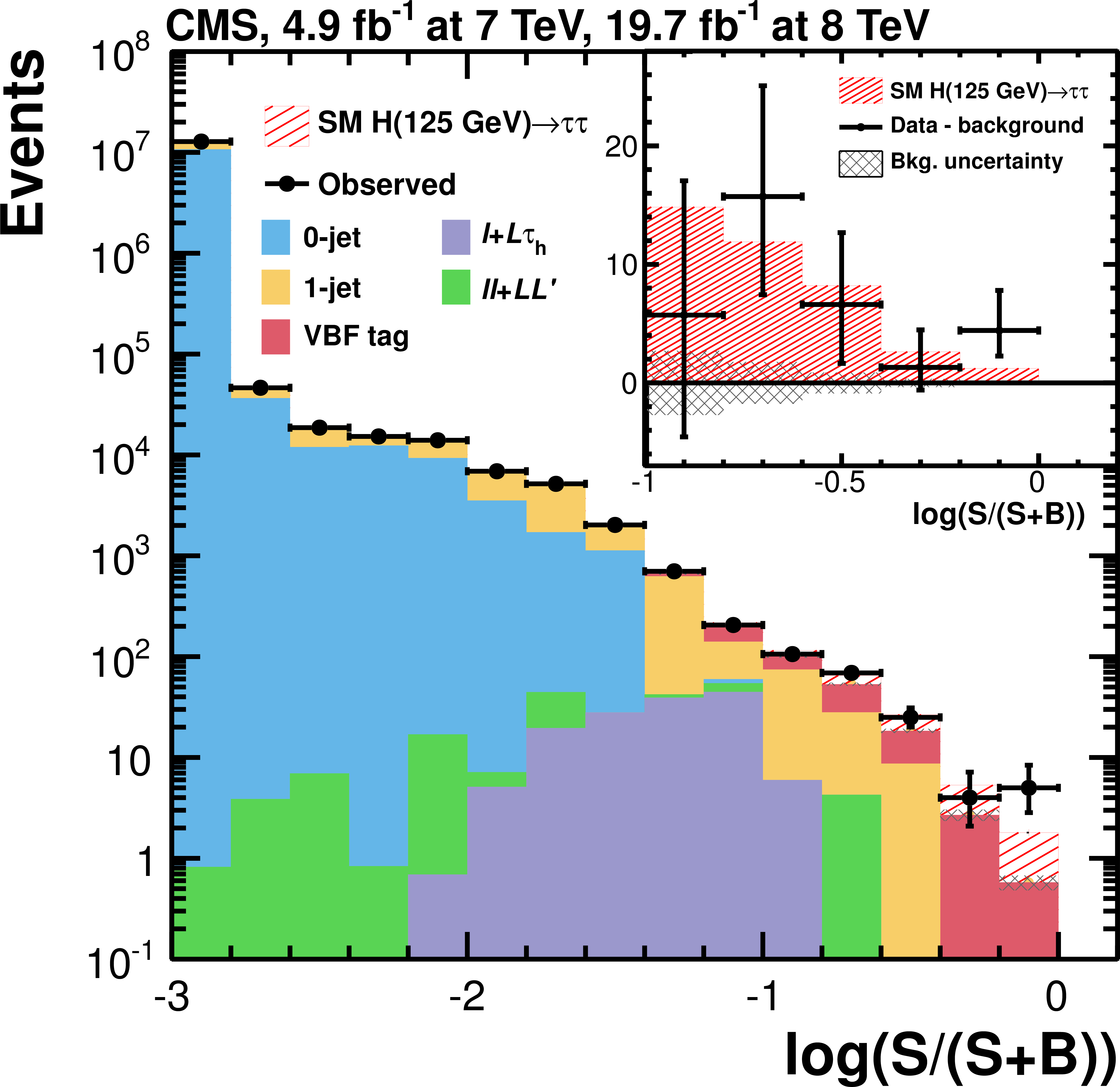
Figure 17:
Combined observed and predicted distributions of the decimal logarithm $\log(S/(S+B))$ in each bin of the final $ {m_{ {\tau } {\tau }}} $, $ {m_\text {vis}} $, or discriminator distributions obtained in all event categories and decay channels, with $S/(S+B)$ denoting the ratio of the predicted signal and signal-plus-background event yields in each bin. The normalization of the predicted background distributions corresponds to the result of the global fit. The signal distribution, on the other hand, is normalized to the SM prediction ($\mu = 1$). The inset shows the corresponding difference between the observed data and expected background distributions, together with the signal distribution for a SM Higgs boson at $ {m_{ {\mathrm {H}} }}$ = 125 GeV. The distribution from SM Higgs boson events in the $ {\mathrm {W}} {\mathrm {W}}$ decay channel does not significantly contribute to this plot. |

png pdf |
Figure 18-a:
Scan of the negative log-likelihood difference, $-2\Delta \ln\mathcal {L}$, as a function of $ {m_{ {\mathrm {H}} }} $ (a) and as a function of $ {\kappa _\mathrm {V}} $ and $ {\kappa _\mathrm {f}} $ (b). For each point, all nuisance parameters are profiled. For the likelihood scan as a function of $ {m_{ {\mathrm {H}} }} $, the background-only hypothesis includes the $ {\mathrm {p}} {\mathrm {p}}\to {\mathrm {H}} \text {(125 GeV)}\to {\mathrm {W}} {\mathrm {W}}$ process for every value of $ {m_{ {\mathrm {H}} }} $. The observation (solid line) is compared to the expectation (dashed line) for a SM Higgs boson with mass $ {m_{ {\mathrm {H}} }} $ = 125 GeV. For the likelihood scan as a function of $ {\kappa _\mathrm {V}} $ and $ {\kappa _\mathrm {f}} $, the $ {\mathrm {H}}\to {\mathrm {W}} {\mathrm {W}}$ contribution is treated as a signal process. |

png pdf |
Figure 18-b:
Scan of the negative log-likelihood difference, $-2\Delta \ln\mathcal {L}$, as a function of $ {m_{ {\mathrm {H}} }} $ (a) and as a function of $ {\kappa _\mathrm {V}} $ and $ {\kappa _\mathrm {f}} $ (b). For each point, all nuisance parameters are profiled. For the likelihood scan as a function of $ {m_{ {\mathrm {H}} }} $, the background-only hypothesis includes the $ {\mathrm {p}} {\mathrm {p}}\to {\mathrm {H}} \text {(125 GeV)}\to {\mathrm {W}} {\mathrm {W}}$ process for every value of $ {m_{ {\mathrm {H}} }} $. The observation (solid line) is compared to the expectation (dashed line) for a SM Higgs boson with mass $ {m_{ {\mathrm {H}} }} $ = 125 GeV. For the likelihood scan as a function of $ {\kappa _\mathrm {V}} $ and $ {\kappa _\mathrm {f}} $, the $ {\mathrm {H}}\to {\mathrm {W}} {\mathrm {W}}$ contribution is treated as a signal process. |
png pdf |
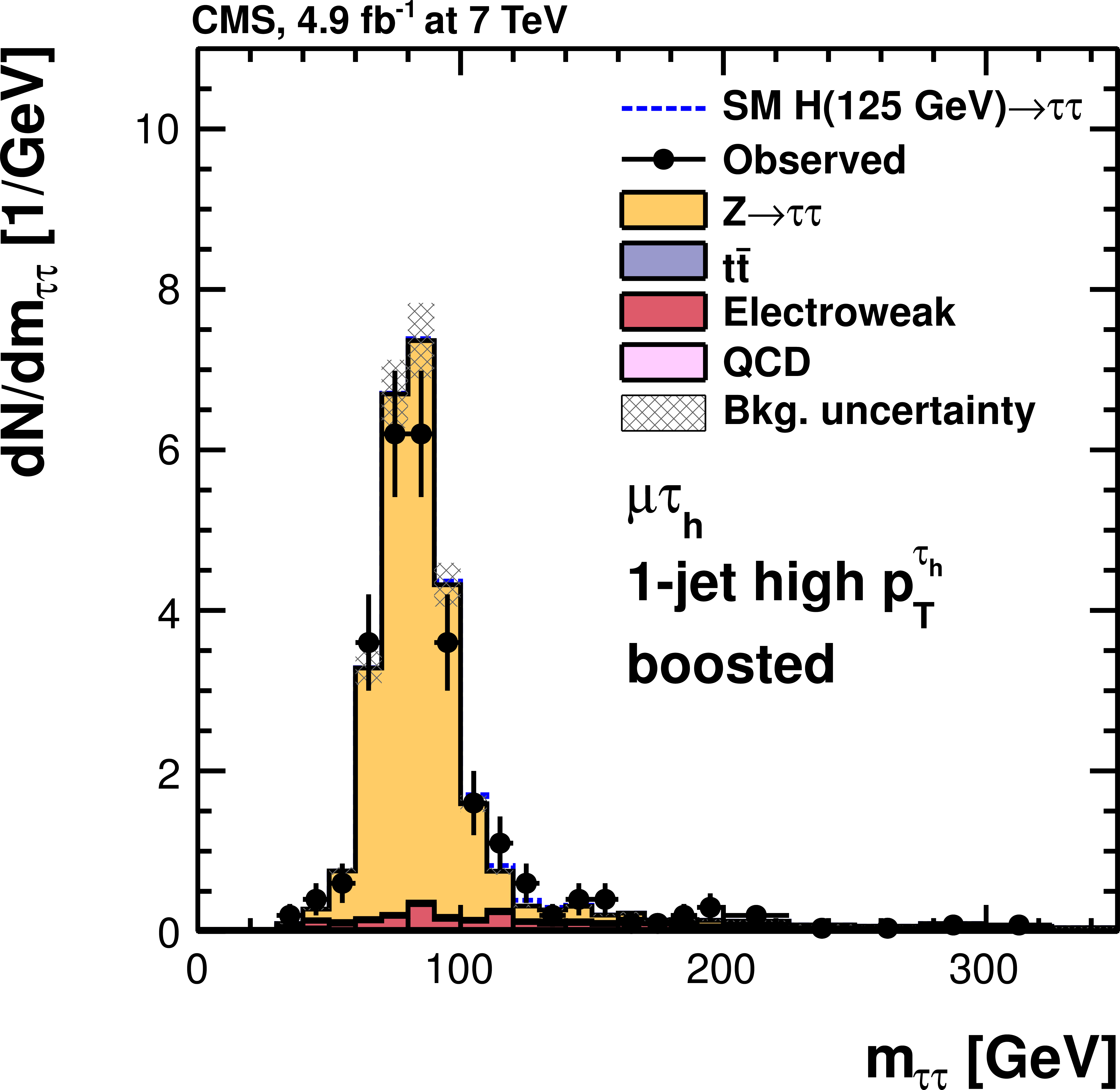
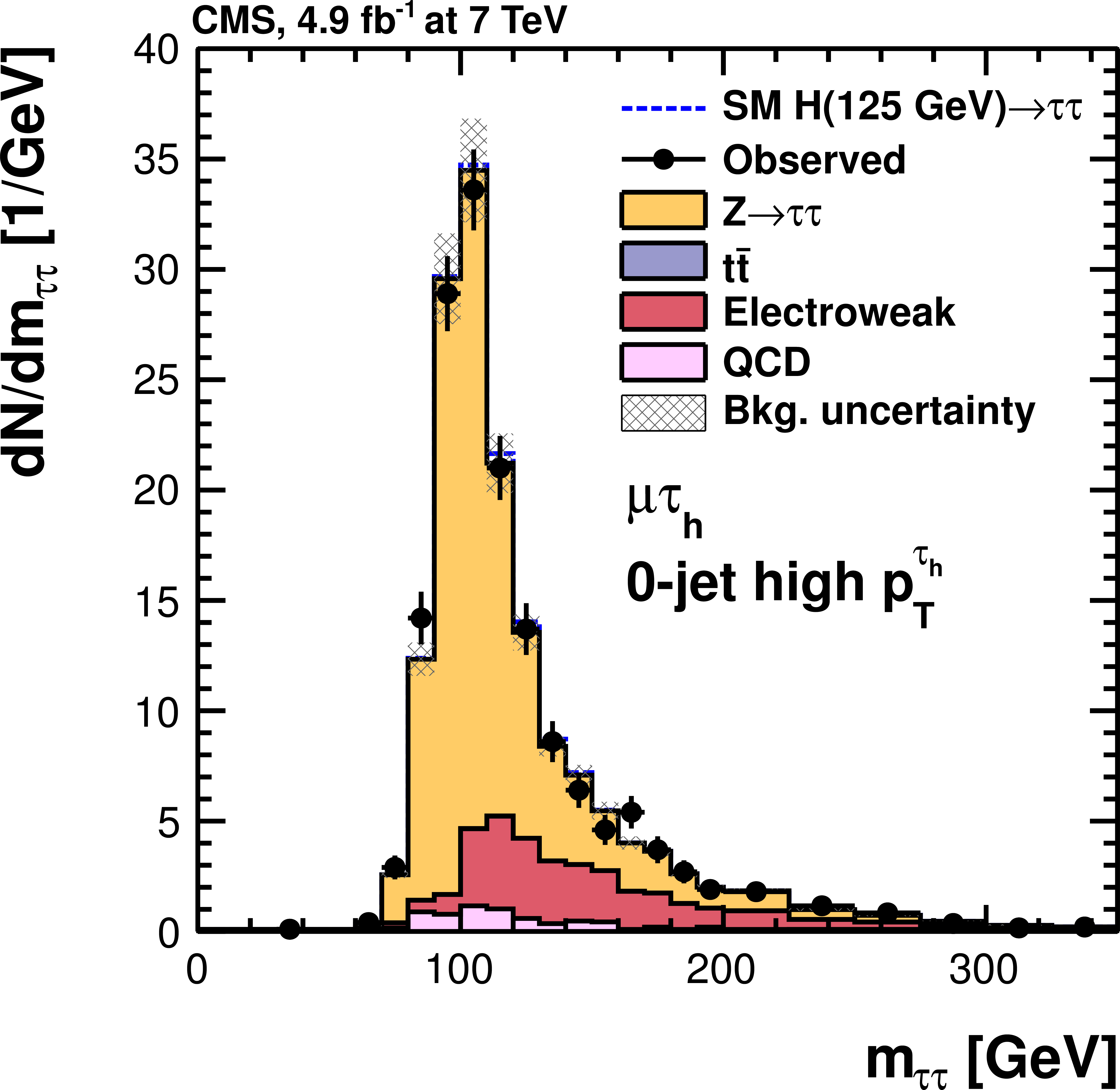
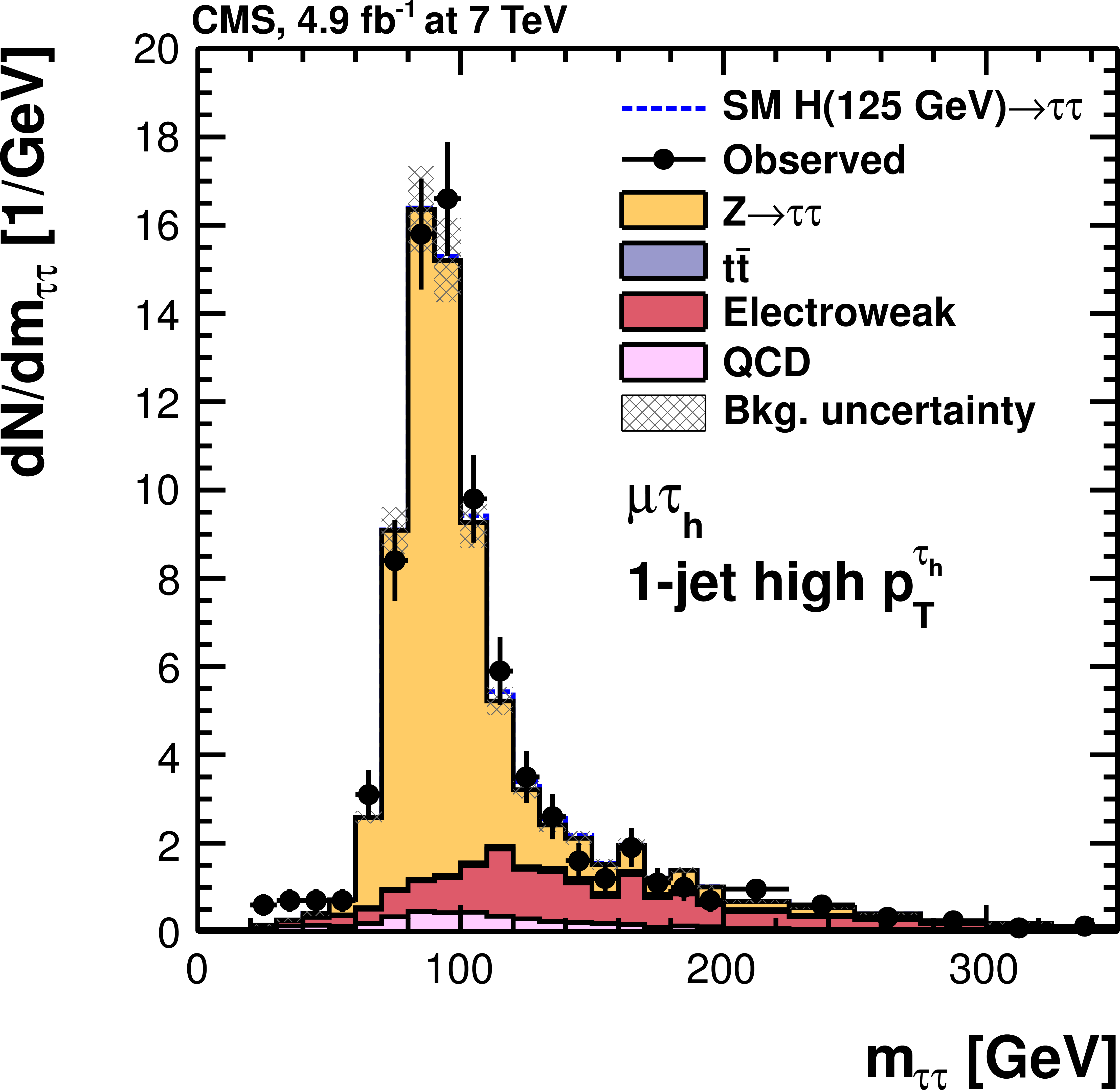
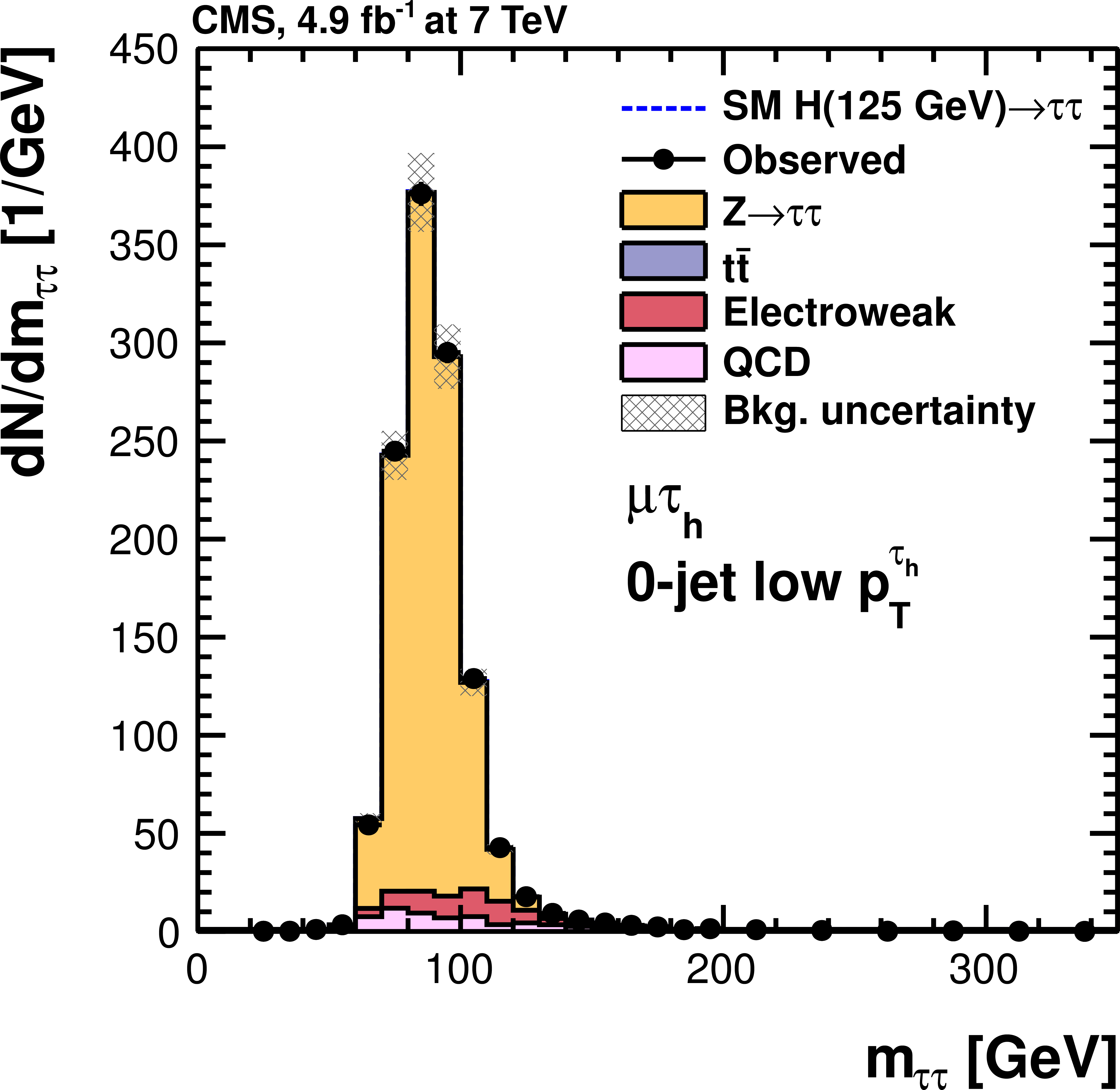
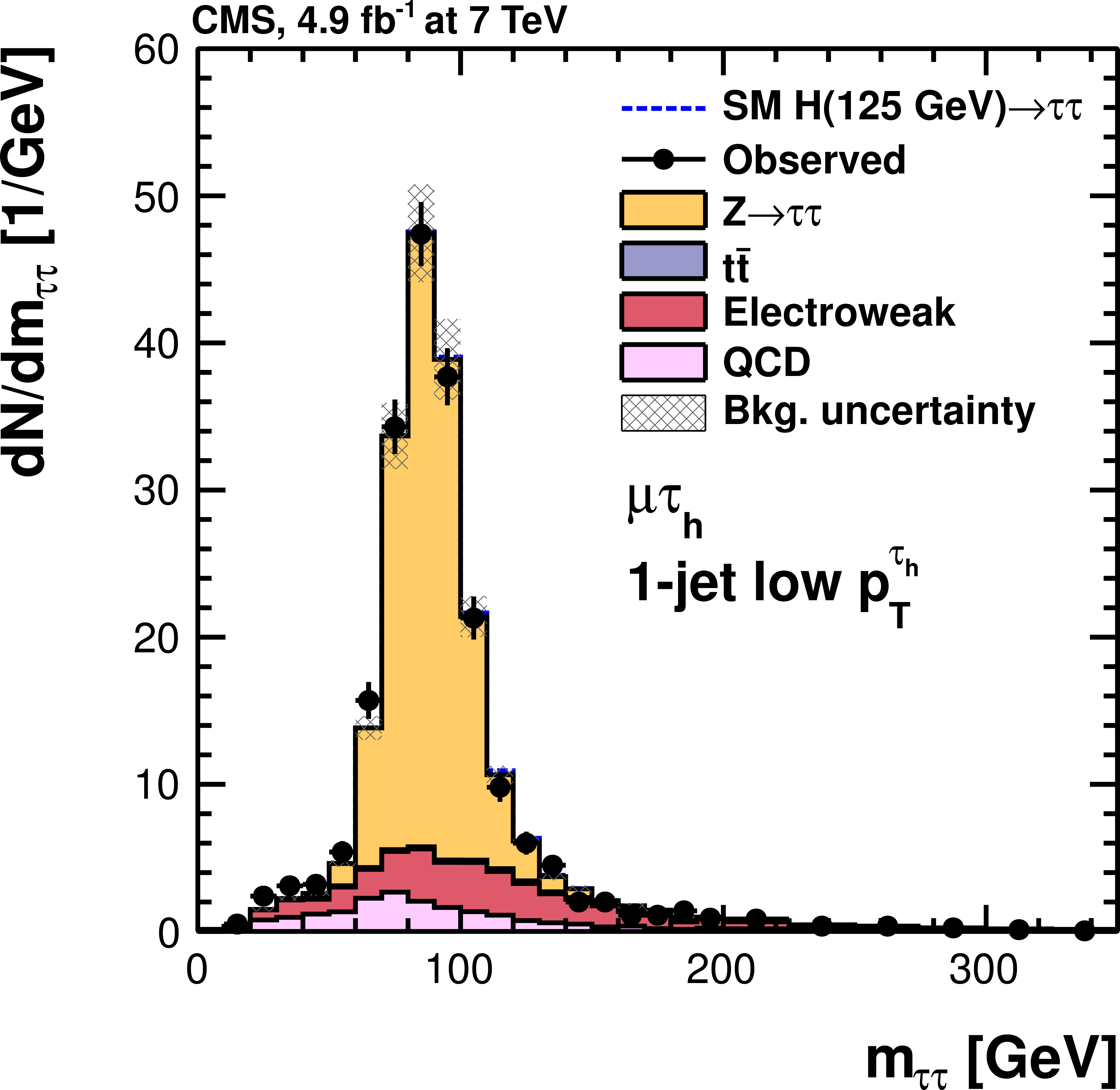
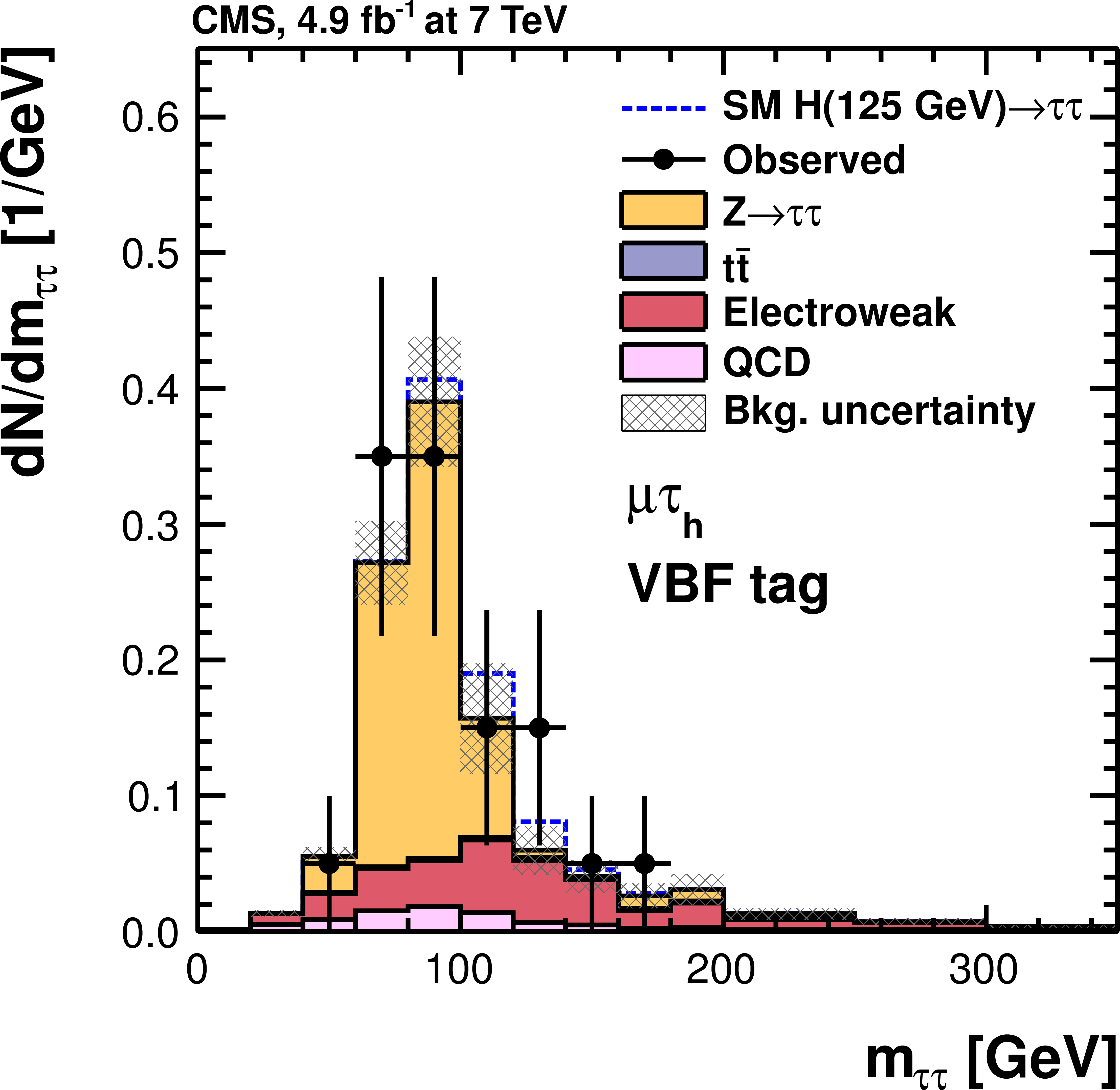
Figure 19-a:
Observed and predicted $ {m_{ {\tau } {\tau }}} $ distributions in the $ {{\mu }} { {\tau }_{\rm h}} $ channel, for all categories used in the 7 TeV data analysis. The normalization of the predicted background distributions corresponds to the result of the global fit. The signal distribution, on the other hand, is normalized to the SM prediction. The signal and background histograms are stacked. |
png pdf |
Figure 19-b:
Observed and predicted $ {m_{ {\tau } {\tau }}} $ distributions in the $ {{\mu }} { {\tau }_{\rm h}} $ channel, for all categories used in the 7 TeV data analysis. The normalization of the predicted background distributions corresponds to the result of the global fit. The signal distribution, on the other hand, is normalized to the SM prediction. The signal and background histograms are stacked. |
png pdf |
Figure 19-c:
Observed and predicted $ {m_{ {\tau } {\tau }}} $ distributions in the $ {{\mu }} { {\tau }_{\rm h}} $ channel, for all categories used in the 7 TeV data analysis. The normalization of the predicted background distributions corresponds to the result of the global fit. The signal distribution, on the other hand, is normalized to the SM prediction. The signal and background histograms are stacked. |
png pdf |
Figure 19-d:
Observed and predicted $ {m_{ {\tau } {\tau }}} $ distributions in the $ {{\mu }} { {\tau }_{\rm h}} $ channel, for all categories used in the 7 TeV data analysis. The normalization of the predicted background distributions corresponds to the result of the global fit. The signal distribution, on the other hand, is normalized to the SM prediction. The signal and background histograms are stacked. |
png pdf |
Figure 19-e:
Observed and predicted $ {m_{ {\tau } {\tau }}} $ distributions in the $ {{\mu }} { {\tau }_{\rm h}} $ channel, for all categories used in the 7 TeV data analysis. The normalization of the predicted background distributions corresponds to the result of the global fit. The signal distribution, on the other hand, is normalized to the SM prediction. The signal and background histograms are stacked. |
png pdf |
Figure 19-f:
Observed and predicted $ {m_{ {\tau } {\tau }}} $ distributions in the $ {{\mu }} { {\tau }_{\rm h}} $ channel, for all categories used in the 7 TeV data analysis. The normalization of the predicted background distributions corresponds to the result of the global fit. The signal distribution, on the other hand, is normalized to the SM prediction. The signal and background histograms are stacked. |
png pdf |
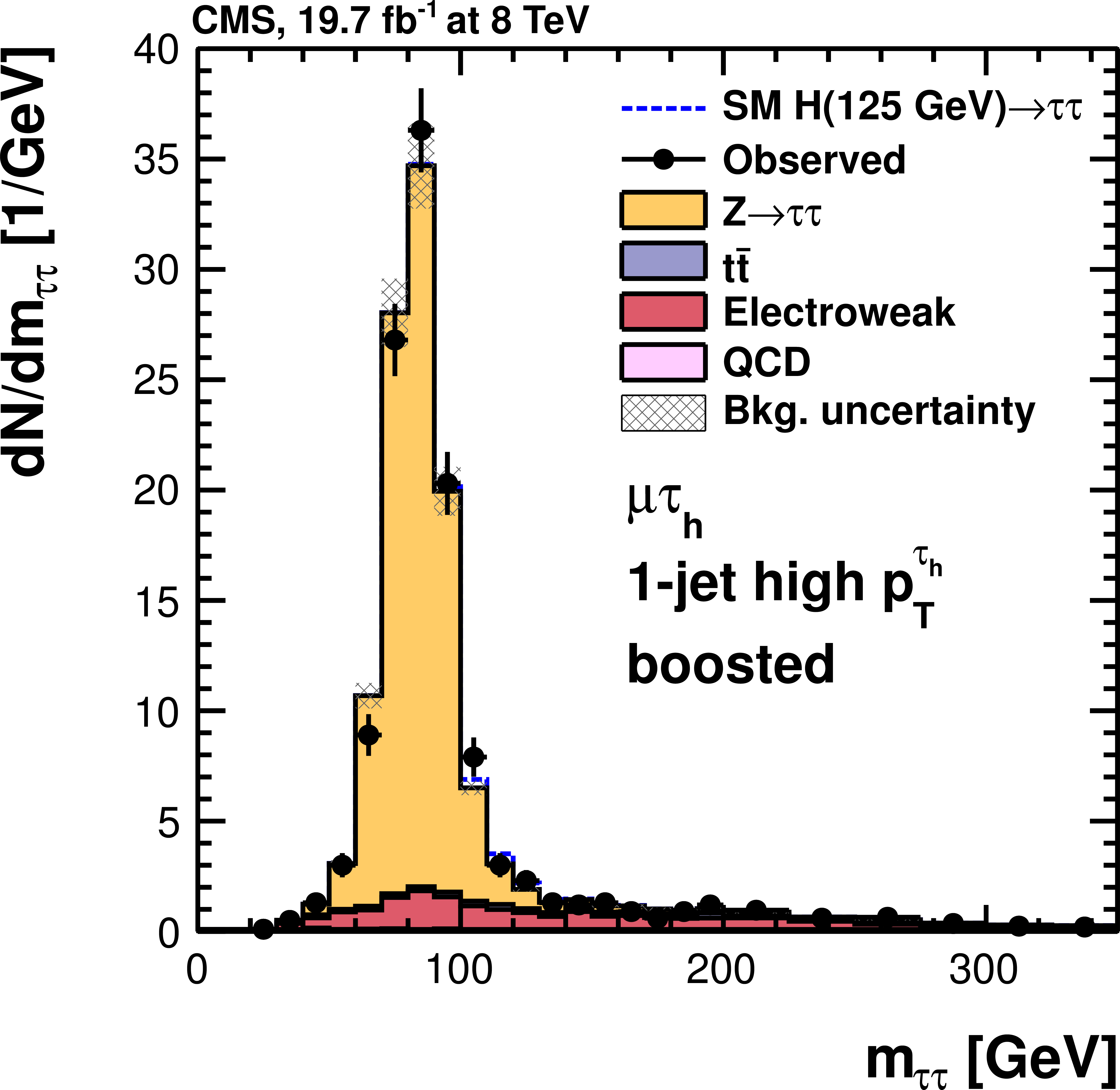
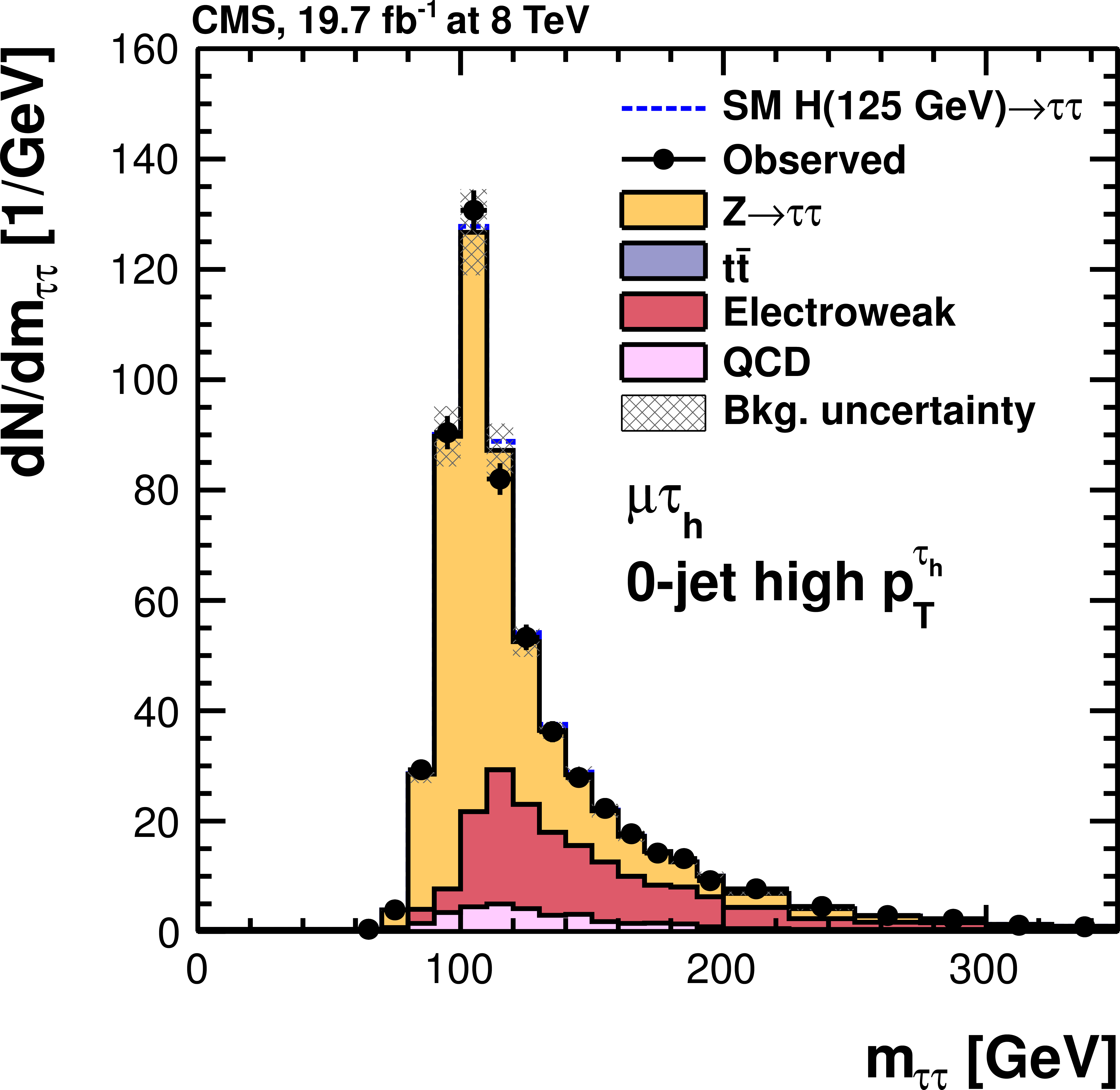
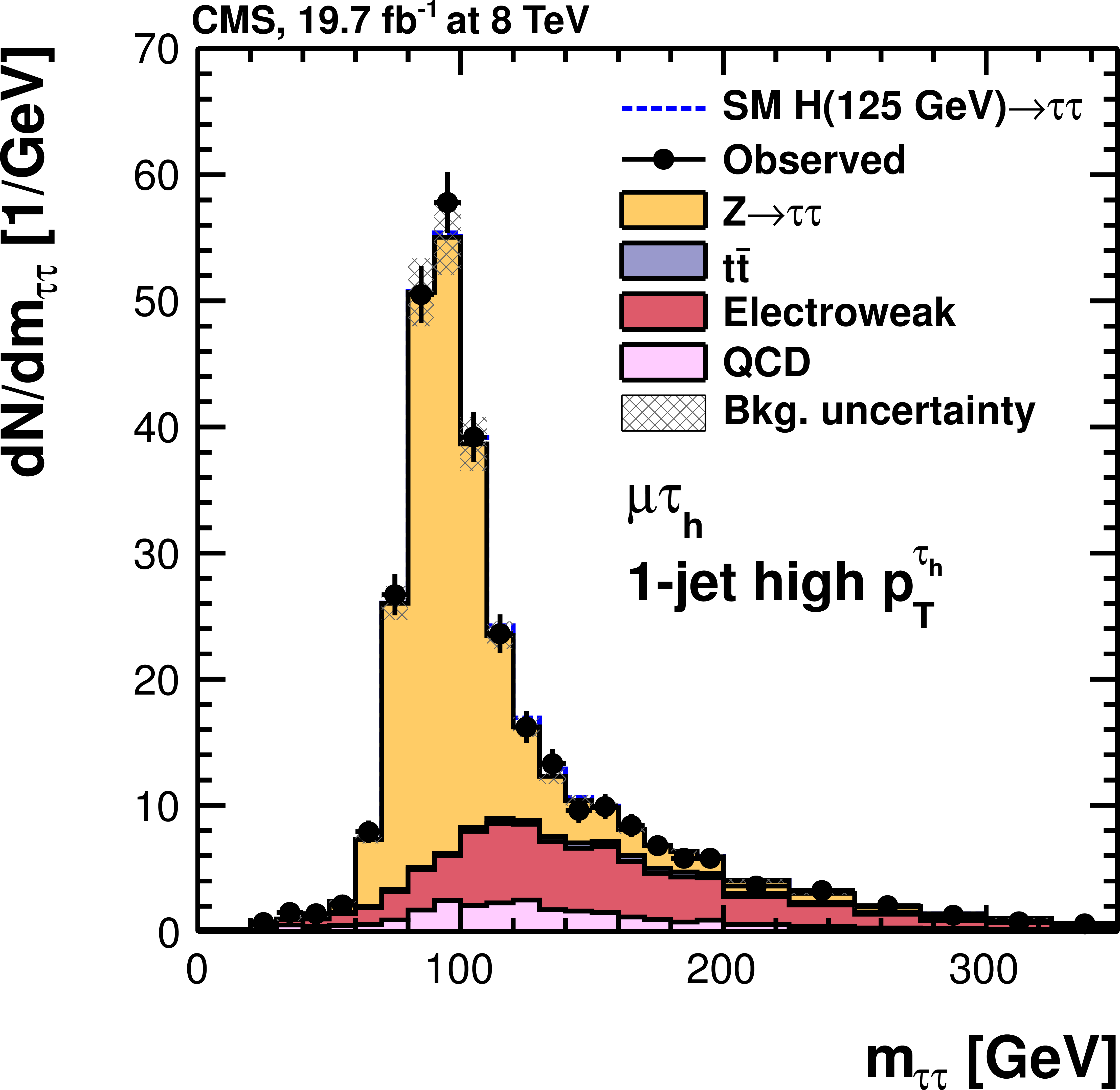
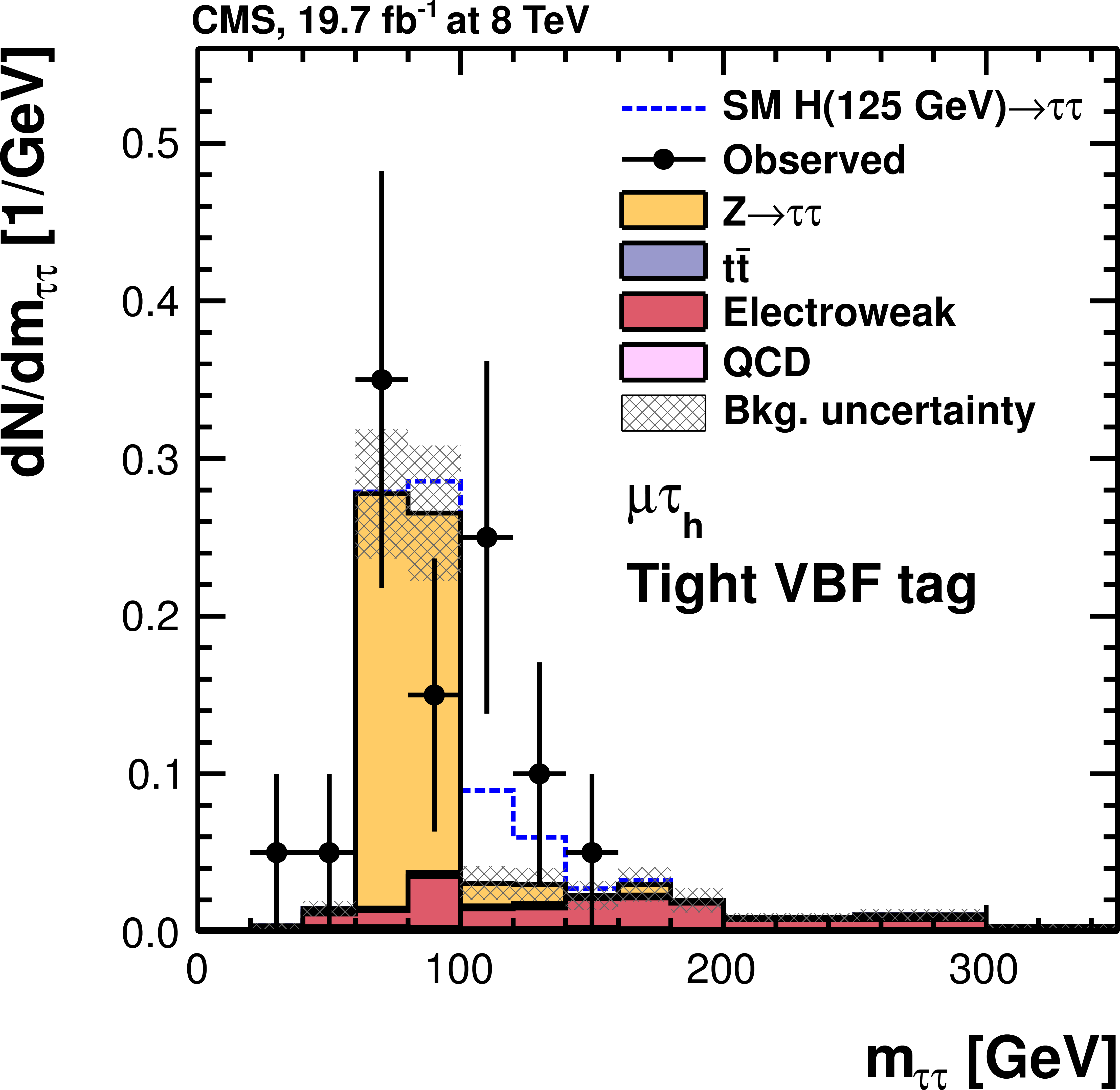
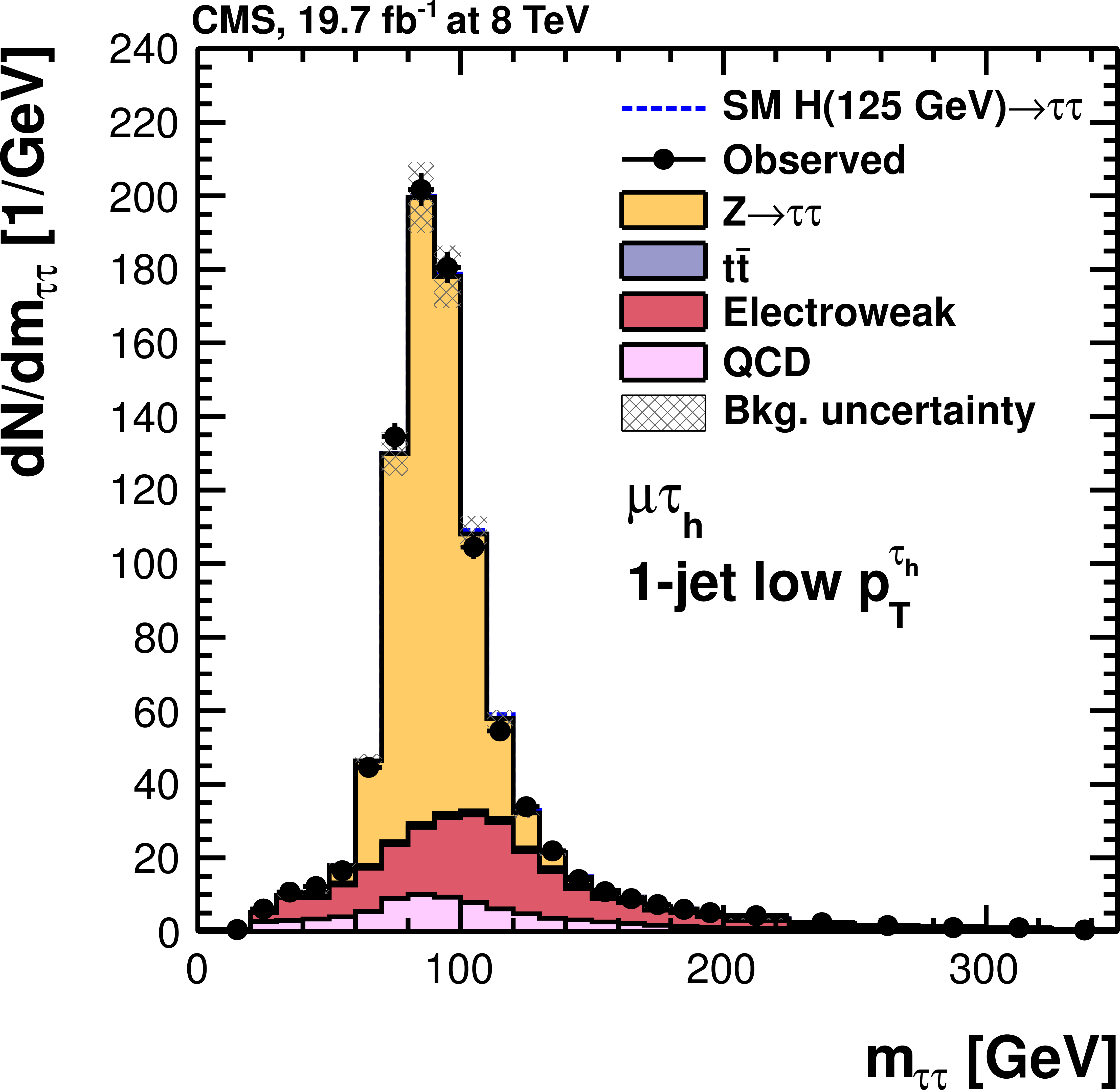
Figure 20-a:
Observed and predicted $ {m_{ {\tau } {\tau }}} $ distributions in the $ {{\mu }} { {\tau }_{\rm h}} $ channel, for all categories used in the 8 TeV data analysis. The normalization of the predicted background distributions corresponds to the result of the global fit. The signal distribution, on the other hand, is normalized to the SM prediction. The signal and background histograms are stacked. |
png pdf |
Figure 20-b:
Observed and predicted $ {m_{ {\tau } {\tau }}} $ distributions in the $ {{\mu }} { {\tau }_{\rm h}} $ channel, for all categories used in the 8 TeV data analysis. The normalization of the predicted background distributions corresponds to the result of the global fit. The signal distribution, on the other hand, is normalized to the SM prediction. The signal and background histograms are stacked. |
png pdf |
Figure 20-c:
Observed and predicted $ {m_{ {\tau } {\tau }}} $ distributions in the $ {{\mu }} { {\tau }_{\rm h}} $ channel, for all categories used in the 8 TeV data analysis. The normalization of the predicted background distributions corresponds to the result of the global fit. The signal distribution, on the other hand, is normalized to the SM prediction. The signal and background histograms are stacked. |
png pdf |
Figure 20-d:
Observed and predicted $ {m_{ {\tau } {\tau }}} $ distributions in the $ {{\mu }} { {\tau }_{\rm h}} $ channel, for all categories used in the 8 TeV data analysis. The normalization of the predicted background distributions corresponds to the result of the global fit. The signal distribution, on the other hand, is normalized to the SM prediction. The signal and background histograms are stacked. |

png pdf |
Figure 20-e:
Observed and predicted $ {m_{ {\tau } {\tau }}} $ distributions in the $ {{\mu }} { {\tau }_{\rm h}} $ channel, for all categories used in the 8 TeV data analysis. The normalization of the predicted background distributions corresponds to the result of the global fit. The signal distribution, on the other hand, is normalized to the SM prediction. The signal and background histograms are stacked. |
png pdf |
Figure 20-f:
Observed and predicted $ {m_{ {\tau } {\tau }}} $ distributions in the $ {{\mu }} { {\tau }_{\rm h}} $ channel, for all categories used in the 8 TeV data analysis. The normalization of the predicted background distributions corresponds to the result of the global fit. The signal distribution, on the other hand, is normalized to the SM prediction. The signal and background histograms are stacked. |
png pdf |
Figure 20-g:
Observed and predicted $ {m_{ {\tau } {\tau }}} $ distributions in the $ {{\mu }} { {\tau }_{\rm h}} $ channel, for all categories used in the 8 TeV data analysis. The normalization of the predicted background distributions corresponds to the result of the global fit. The signal distribution, on the other hand, is normalized to the SM prediction. The signal and background histograms are stacked. |
png pdf |
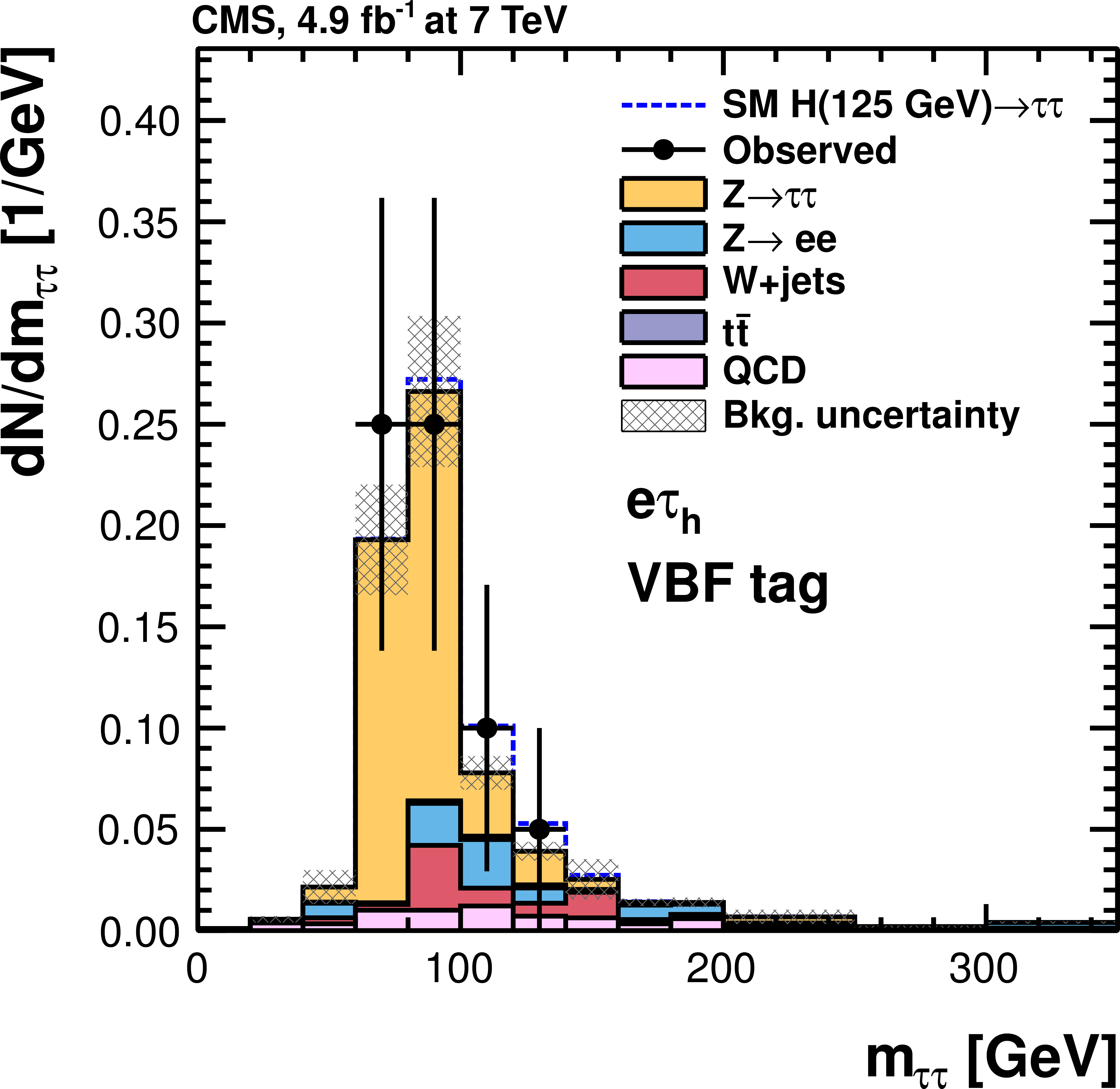
Figure 21-a:
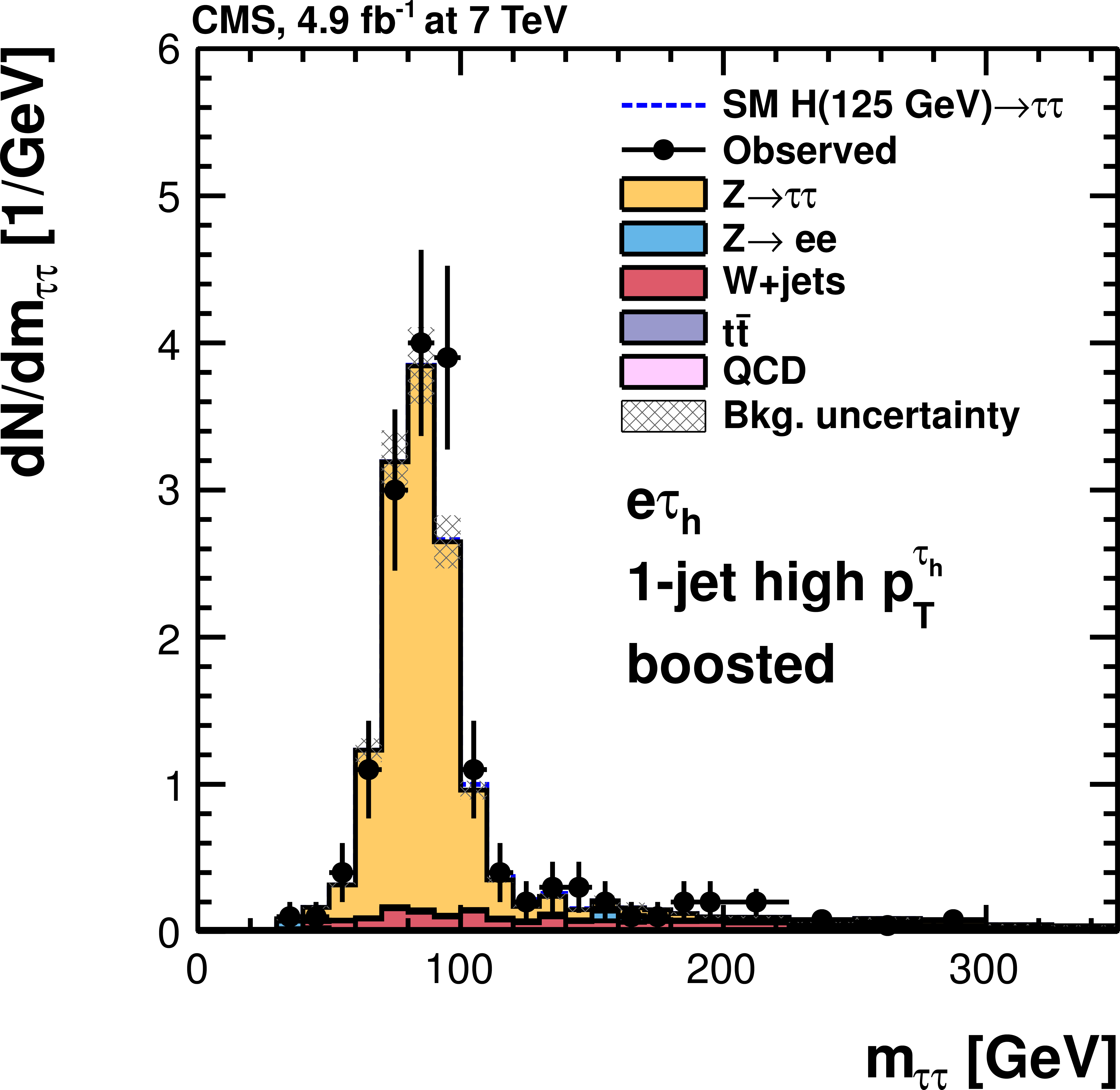
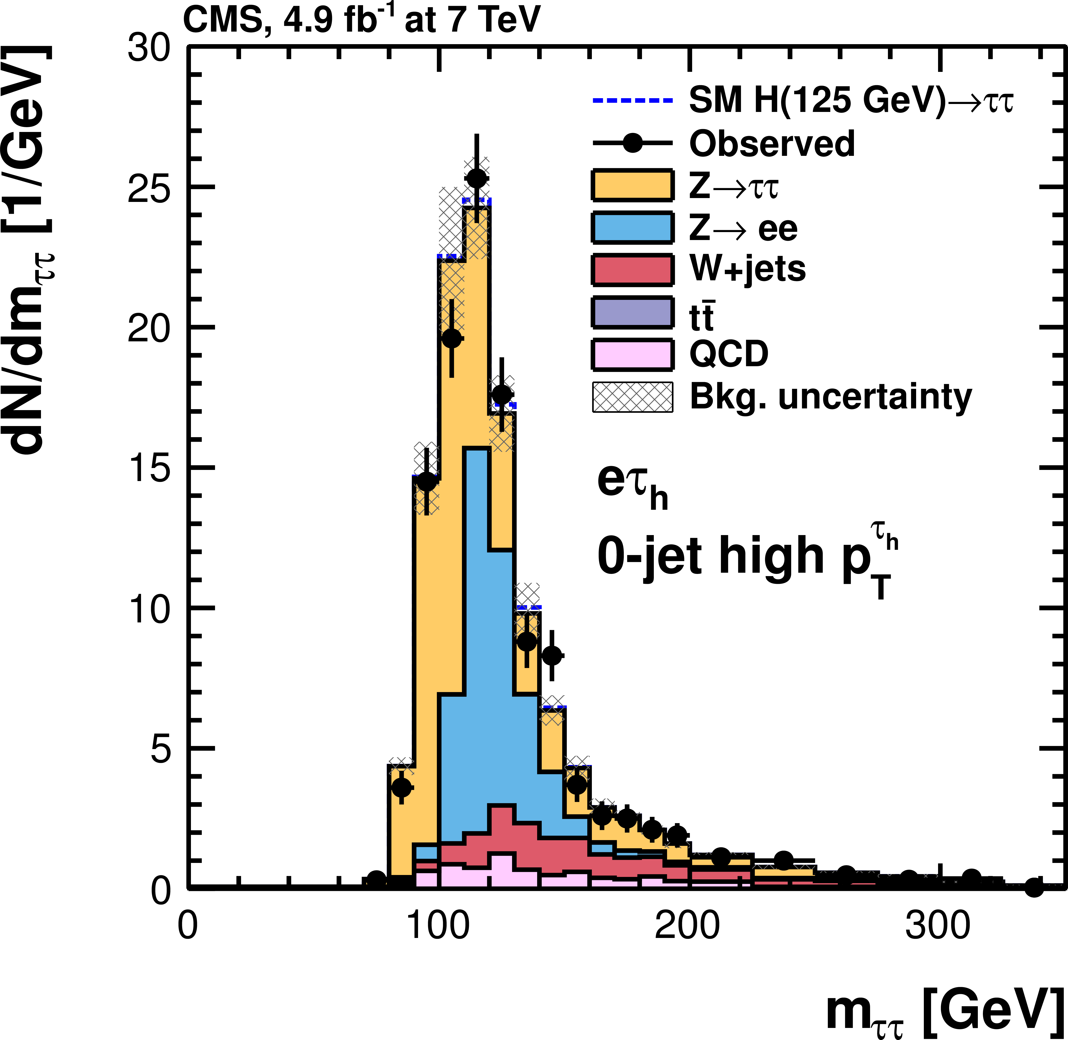
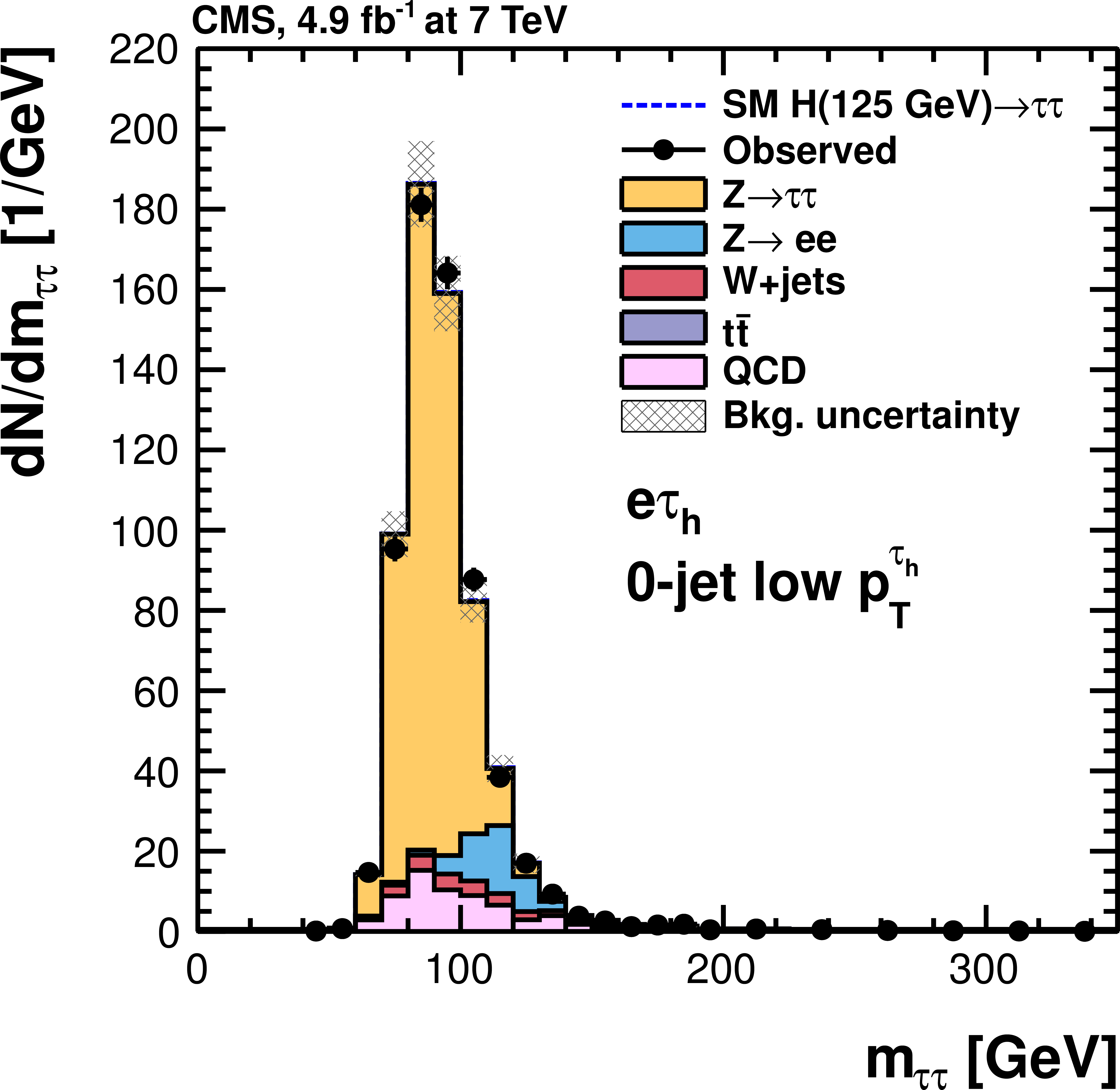
Observed and predicted $ {m_{ {\tau } {\tau }}} $ distributions in the $ {\mathrm {e}} { {\tau }_{\rm h}} $ channel, for all categories used in the 7 TeV data analysis. The normalization of the predicted background distributions corresponds to the result of the global fit. The signal distribution, on the other hand, is normalized to the SM prediction. The signal and background histograms are stacked. |
png pdf |
Figure 21-b:
Observed and predicted $ {m_{ {\tau } {\tau }}} $ distributions in the $ {\mathrm {e}} { {\tau }_{\rm h}} $ channel, for all categories used in the 7 TeV data analysis. The normalization of the predicted background distributions corresponds to the result of the global fit. The signal distribution, on the other hand, is normalized to the SM prediction. The signal and background histograms are stacked. |
png pdf |
Figure 21-c:
Observed and predicted $ {m_{ {\tau } {\tau }}} $ distributions in the $ {\mathrm {e}} { {\tau }_{\rm h}} $ channel, for all categories used in the 7 TeV data analysis. The normalization of the predicted background distributions corresponds to the result of the global fit. The signal distribution, on the other hand, is normalized to the SM prediction. The signal and background histograms are stacked. |

png pdf |
Figure 21-d:
Observed and predicted $ {m_{ {\tau } {\tau }}} $ distributions in the $ {\mathrm {e}} { {\tau }_{\rm h}} $ channel, for all categories used in the 7 TeV data analysis. The normalization of the predicted background distributions corresponds to the result of the global fit. The signal distribution, on the other hand, is normalized to the SM prediction. The signal and background histograms are stacked. |
png pdf |
Figure 21-e:
Observed and predicted $ {m_{ {\tau } {\tau }}} $ distributions in the $ {\mathrm {e}} { {\tau }_{\rm h}} $ channel, for all categories used in the 7 TeV data analysis. The normalization of the predicted background distributions corresponds to the result of the global fit. The signal distribution, on the other hand, is normalized to the SM prediction. The signal and background histograms are stacked. |

png pdf |
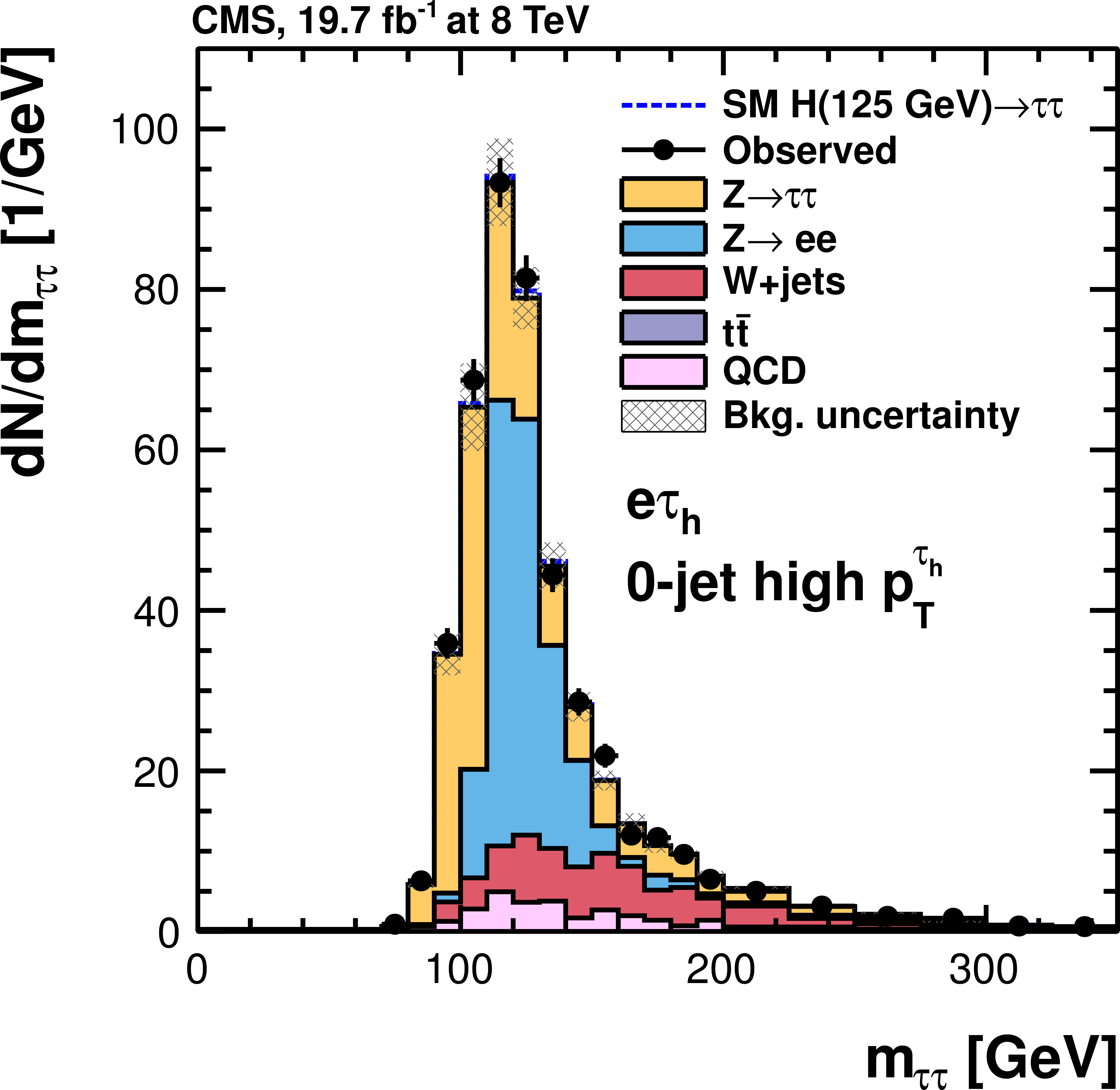
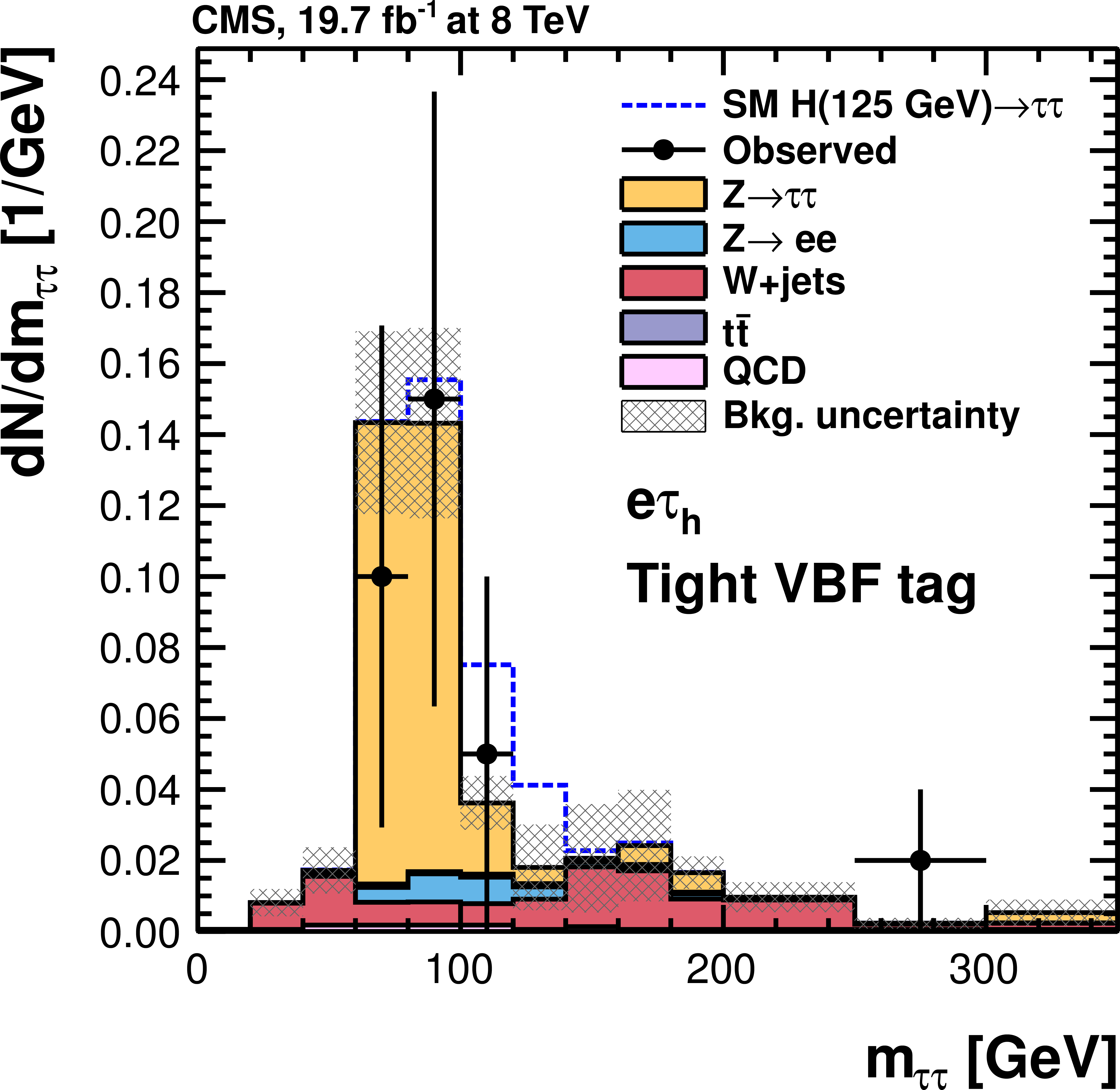
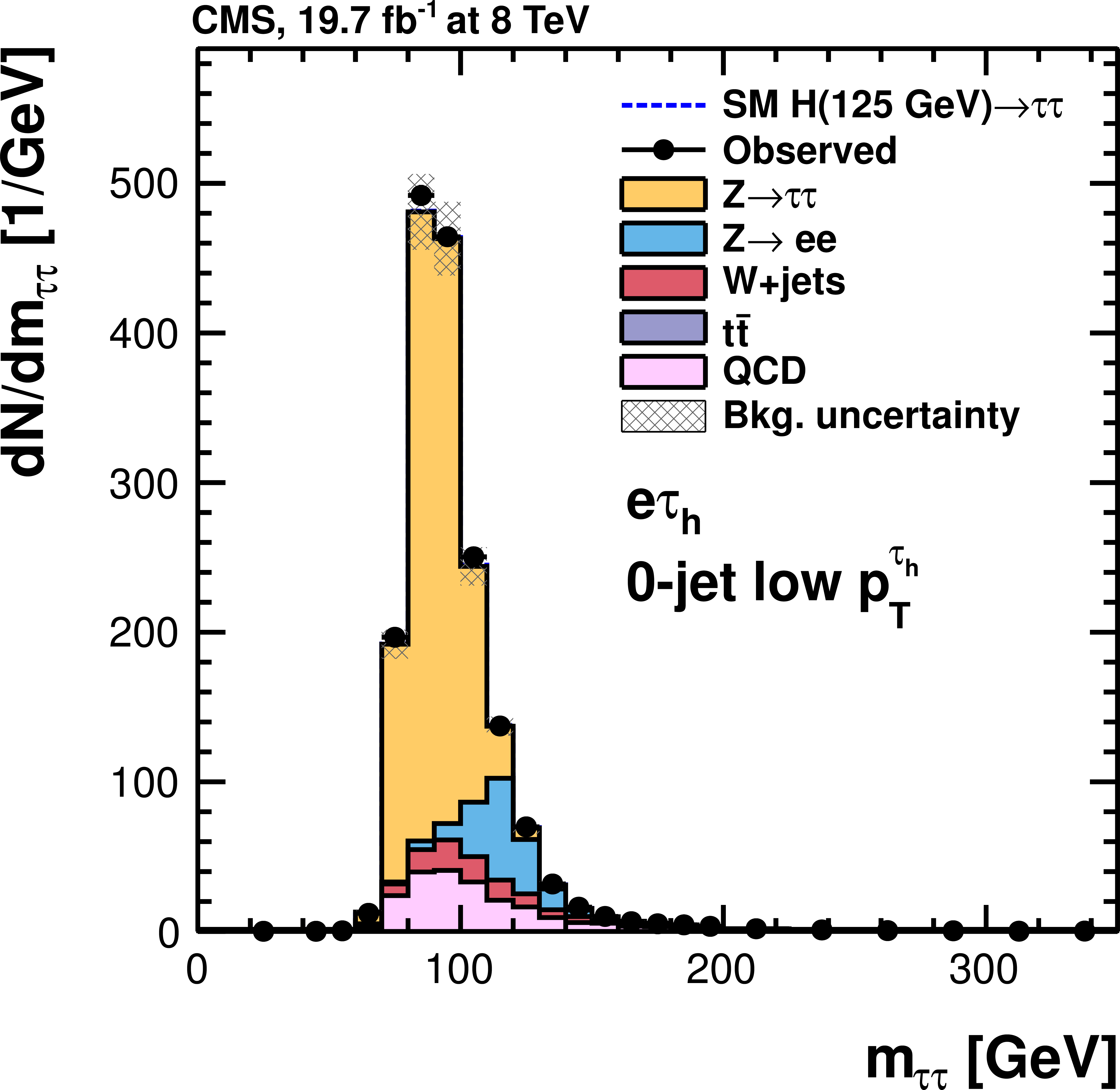
Figure 22-a:
Observed and predicted $ {m_{ {\tau } {\tau }}} $ distributions in the $ {\mathrm {e}} { {\tau }_{\rm h}} $ channel, for all categories used in the 8 TeV data analysis. The normalization of the predicted background distributions corresponds to the result of the global fit. The signal distribution, on the other hand, is normalized to the SM prediction. The signal and background histograms are stacked. |
png pdf |
Figure 22-b:
Observed and predicted $ {m_{ {\tau } {\tau }}} $ distributions in the $ {\mathrm {e}} { {\tau }_{\rm h}} $ channel, for all categories used in the 8 TeV data analysis. The normalization of the predicted background distributions corresponds to the result of the global fit. The signal distribution, on the other hand, is normalized to the SM prediction. The signal and background histograms are stacked. |
png pdf |
Figure 22-c:
Observed and predicted $ {m_{ {\tau } {\tau }}} $ distributions in the $ {\mathrm {e}} { {\tau }_{\rm h}} $ channel, for all categories used in the 8 TeV data analysis. The normalization of the predicted background distributions corresponds to the result of the global fit. The signal distribution, on the other hand, is normalized to the SM prediction. The signal and background histograms are stacked. |
png pdf |
Figure 22-d:
Observed and predicted $ {m_{ {\tau } {\tau }}} $ distributions in the $ {\mathrm {e}} { {\tau }_{\rm h}} $ channel, for all categories used in the 8 TeV data analysis. The normalization of the predicted background distributions corresponds to the result of the global fit. The signal distribution, on the other hand, is normalized to the SM prediction. The signal and background histograms are stacked. |

png pdf |
Figure 22-e:
Observed and predicted $ {m_{ {\tau } {\tau }}} $ distributions in the $ {\mathrm {e}} { {\tau }_{\rm h}} $ channel, for all categories used in the 8 TeV data analysis. The normalization of the predicted background distributions corresponds to the result of the global fit. The signal distribution, on the other hand, is normalized to the SM prediction. The signal and background histograms are stacked. |
png pdf |
Figure 22-f:
Observed and predicted $ {m_{ {\tau } {\tau }}} $ distributions in the $ {\mathrm {e}} { {\tau }_{\rm h}} $ channel, for all categories used in the 8 TeV data analysis. The normalization of the predicted background distributions corresponds to the result of the global fit. The signal distribution, on the other hand, is normalized to the SM prediction. The signal and background histograms are stacked. |
png pdf |
Figure 23-a:
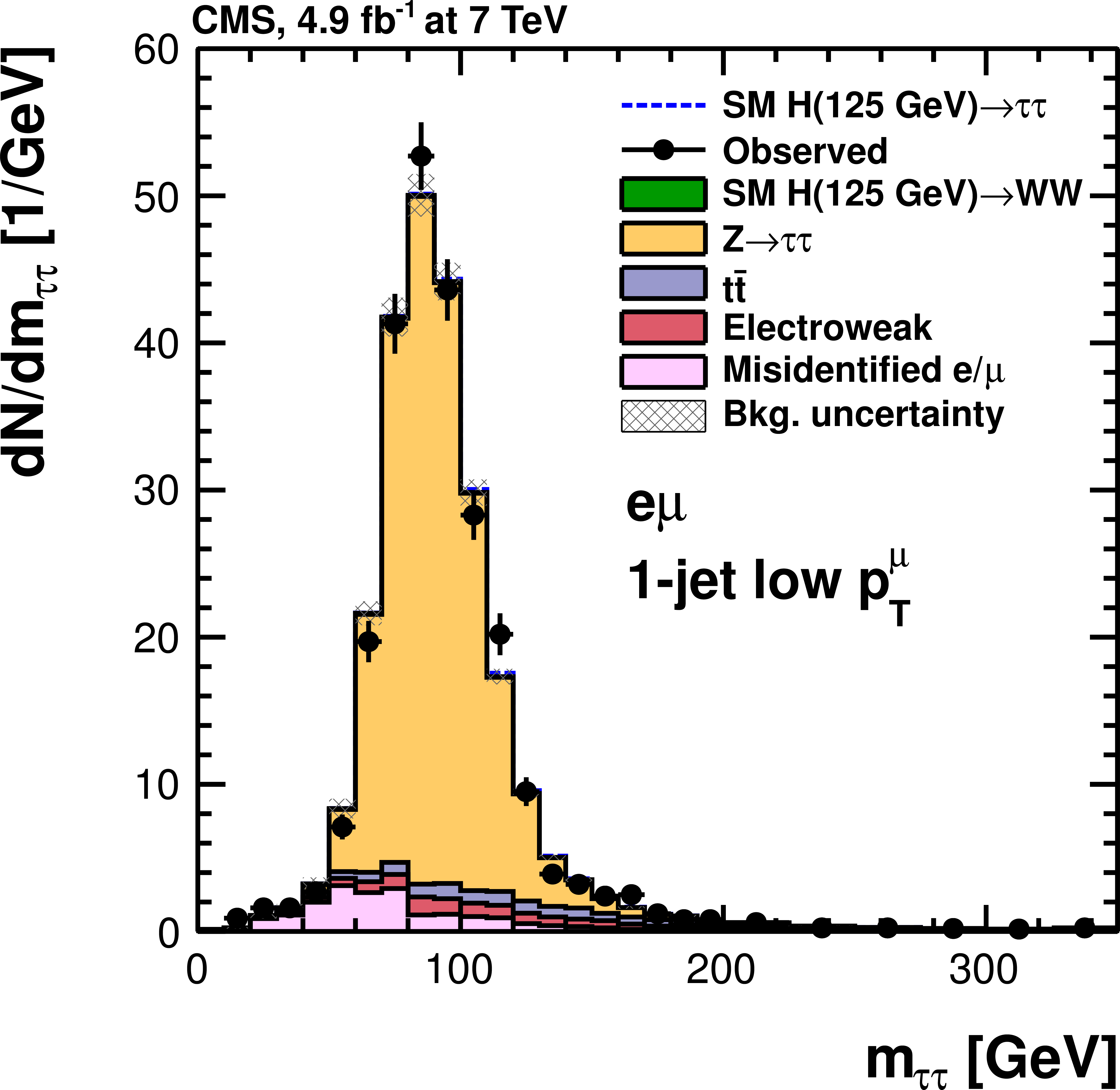
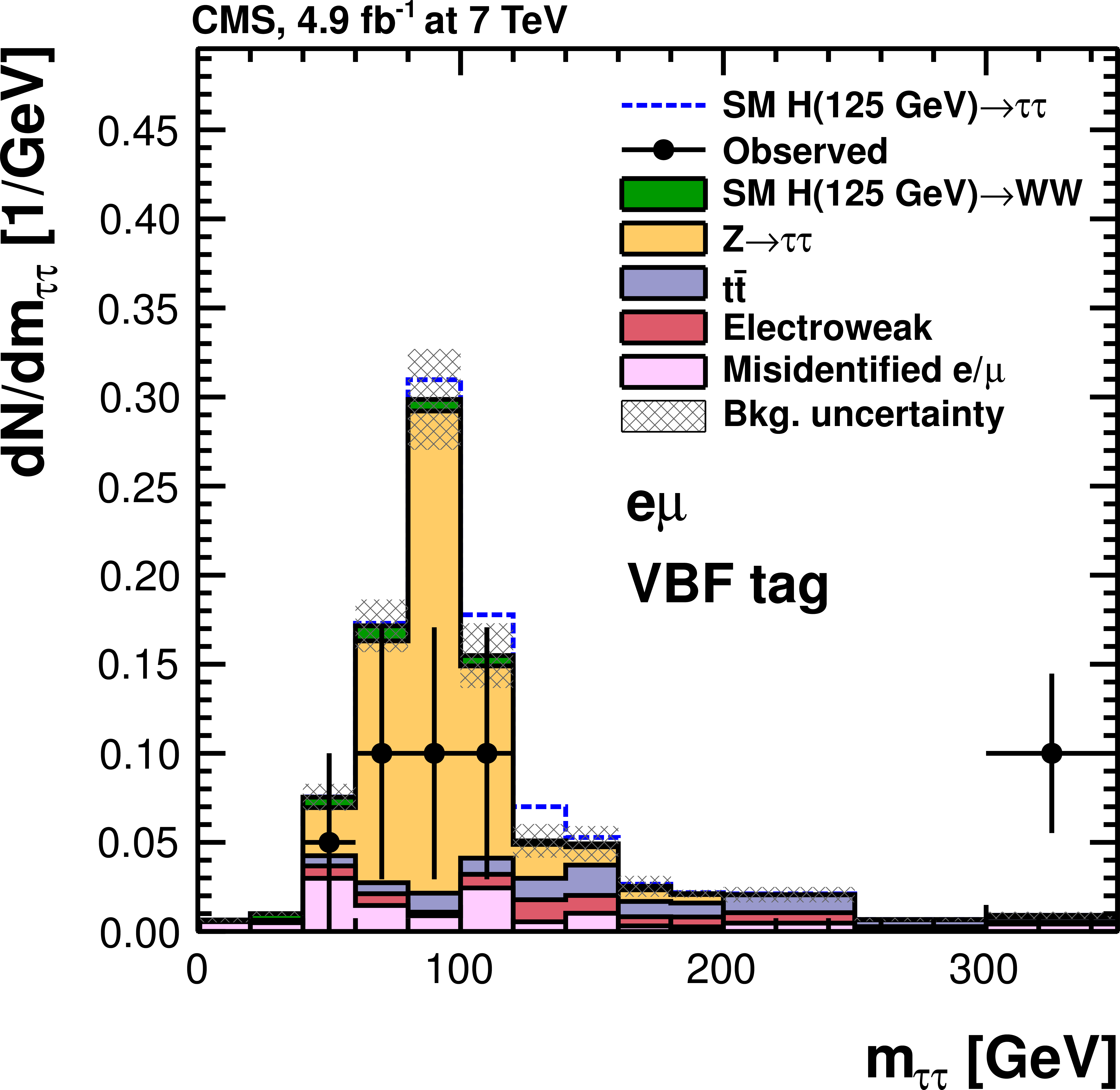
Observed and predicted $ {m_{ {\tau } {\tau }}} $ distributions in the $ {\mathrm {e}} {{\mu }}$ channel, for all categories used in the 7 TeV data analysis. The normalization of the predicted background distributions corresponds to the result of the global fit. The signal distribution, on the other hand, is normalized to the SM prediction. The signal and background histograms are stacked. |
png pdf |
Figure 23-b:
Observed and predicted $ {m_{ {\tau } {\tau }}} $ distributions in the $ {\mathrm {e}} {{\mu }}$ channel, for all categories used in the 7 TeV data analysis. The normalization of the predicted background distributions corresponds to the result of the global fit. The signal distribution, on the other hand, is normalized to the SM prediction. The signal and background histograms are stacked. |
png pdf |
Figure 23-c:
Observed and predicted $ {m_{ {\tau } {\tau }}} $ distributions in the $ {\mathrm {e}} {{\mu }}$ channel, for all categories used in the 7 TeV data analysis. The normalization of the predicted background distributions corresponds to the result of the global fit. The signal distribution, on the other hand, is normalized to the SM prediction. The signal and background histograms are stacked. |
png pdf |
Figure 23-d:
Observed and predicted $ {m_{ {\tau } {\tau }}} $ distributions in the $ {\mathrm {e}} {{\mu }}$ channel, for all categories used in the 7 TeV data analysis. The normalization of the predicted background distributions corresponds to the result of the global fit. The signal distribution, on the other hand, is normalized to the SM prediction. The signal and background histograms are stacked. |
png pdf |
Figure 23-e:
Observed and predicted $ {m_{ {\tau } {\tau }}} $ distributions in the $ {\mathrm {e}} {{\mu }}$ channel, for all categories used in the 7 TeV data analysis. The normalization of the predicted background distributions corresponds to the result of the global fit. The signal distribution, on the other hand, is normalized to the SM prediction. The signal and background histograms are stacked. |
png pdf |
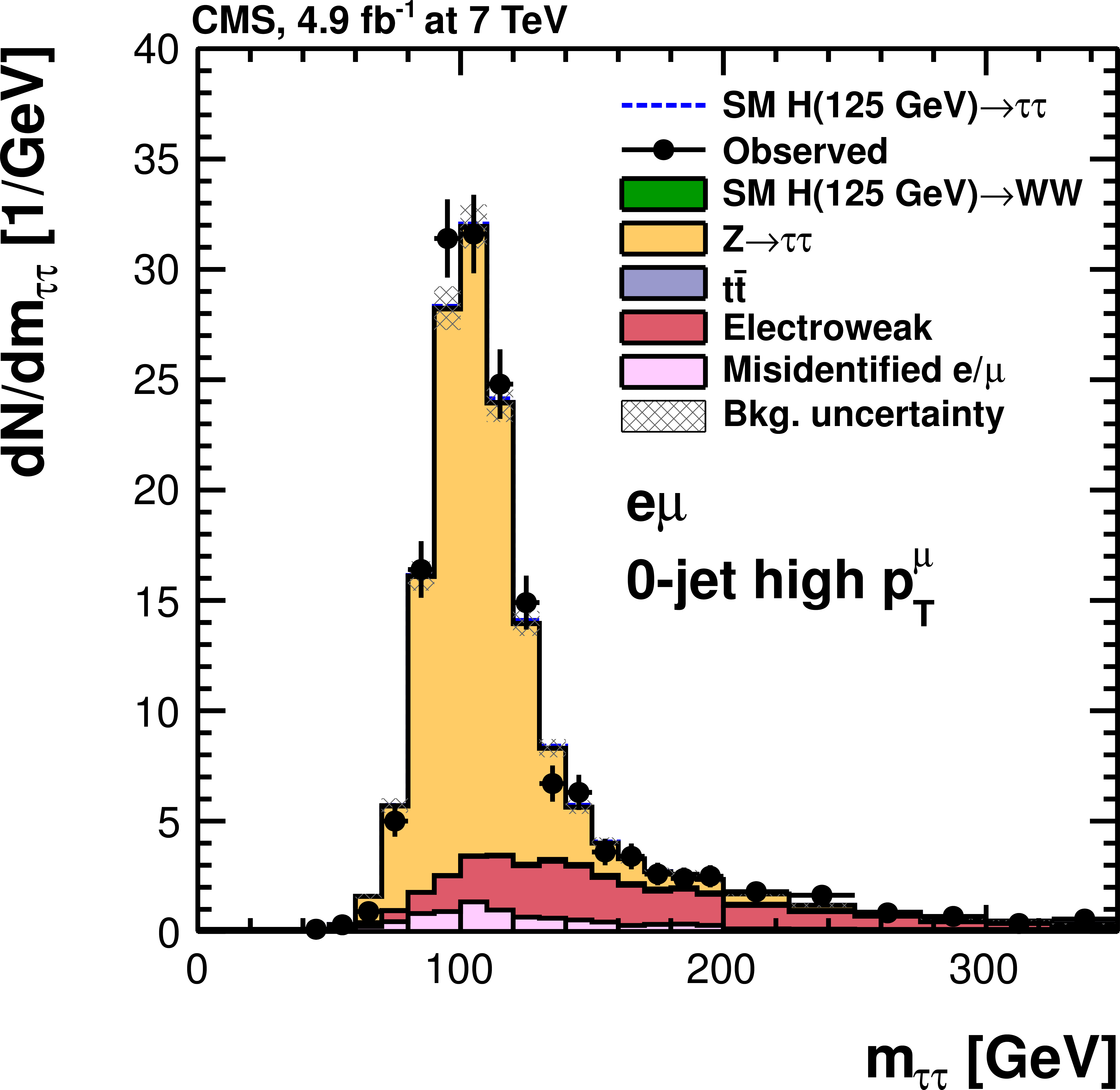
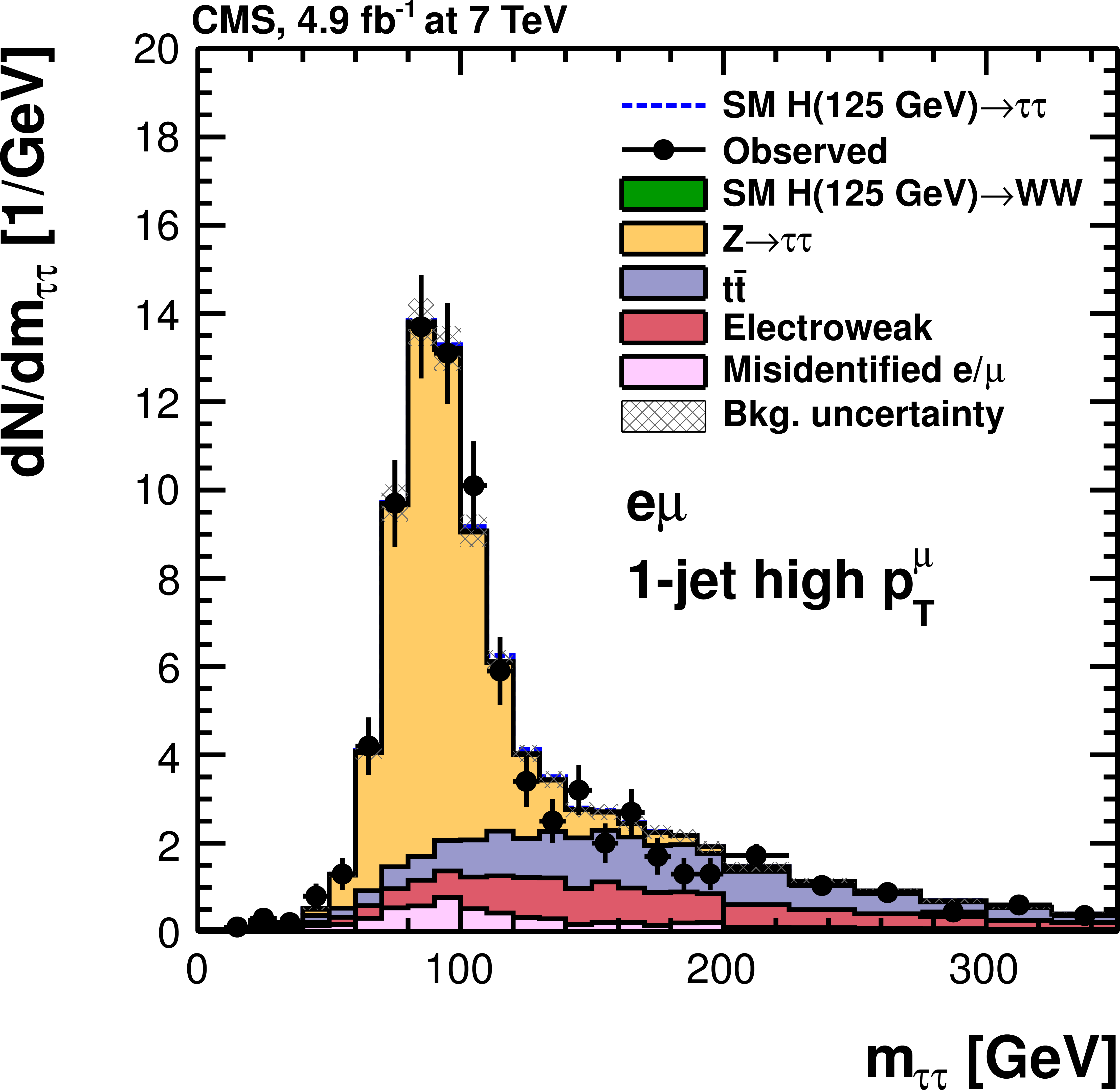
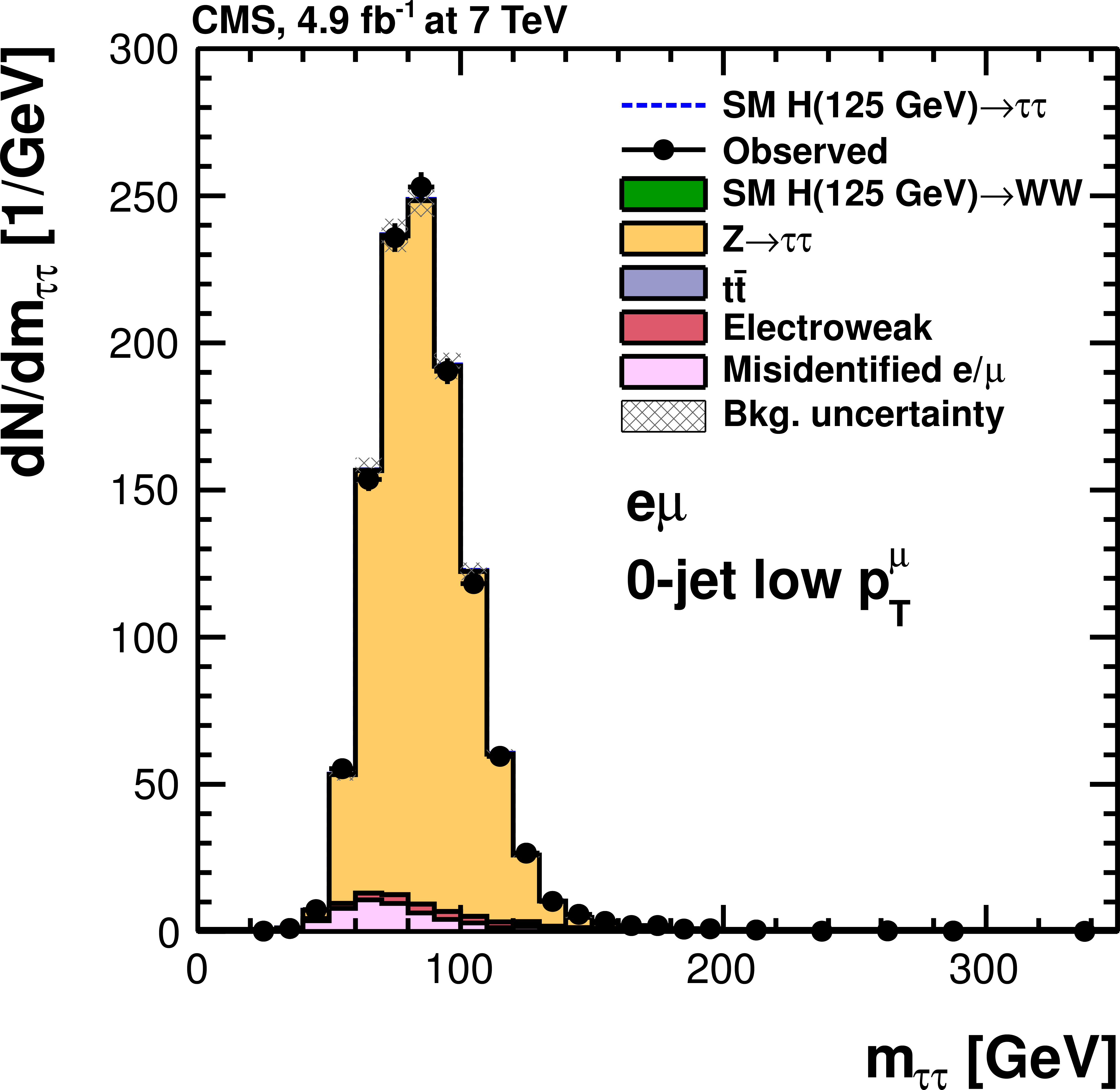
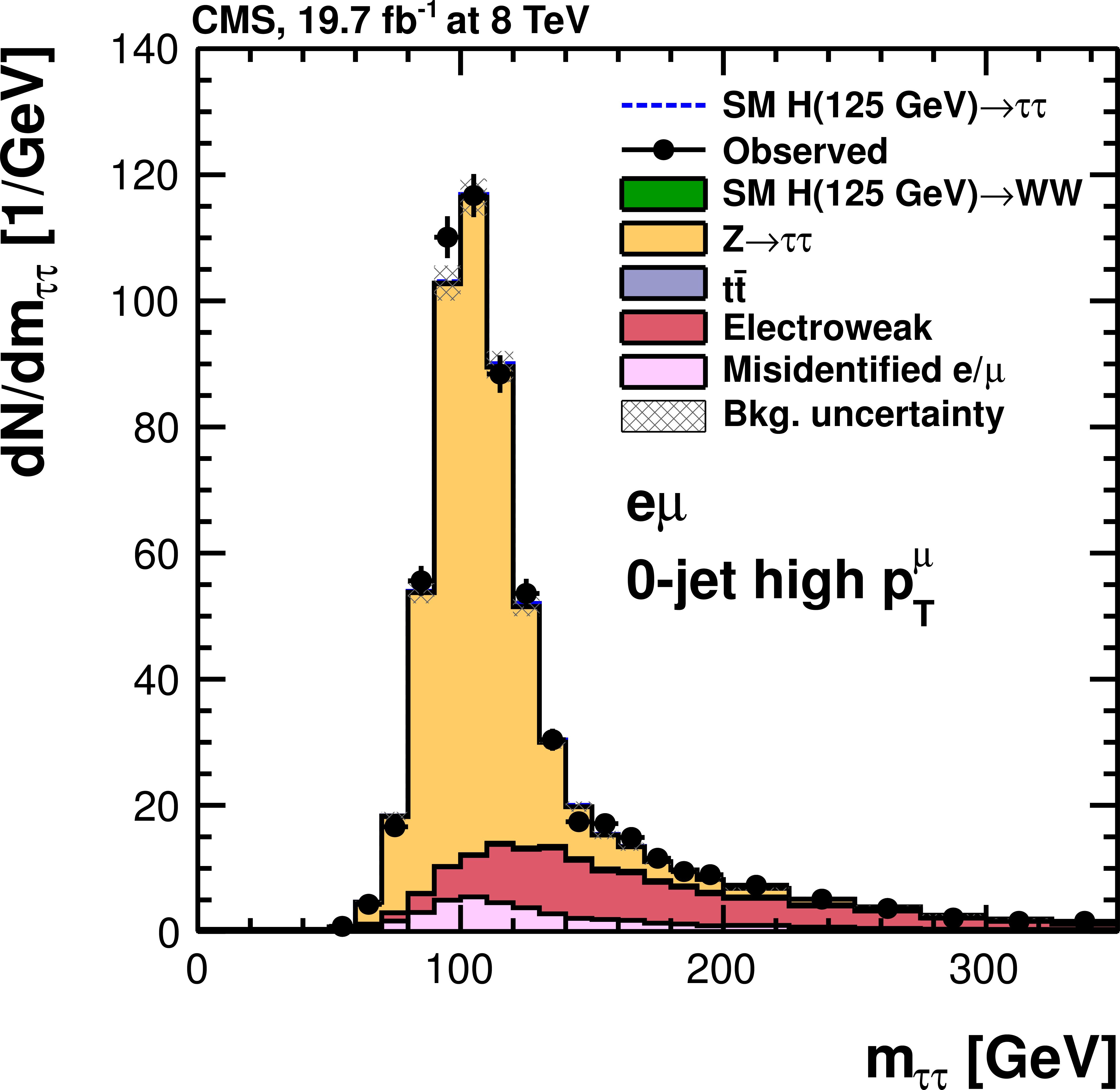
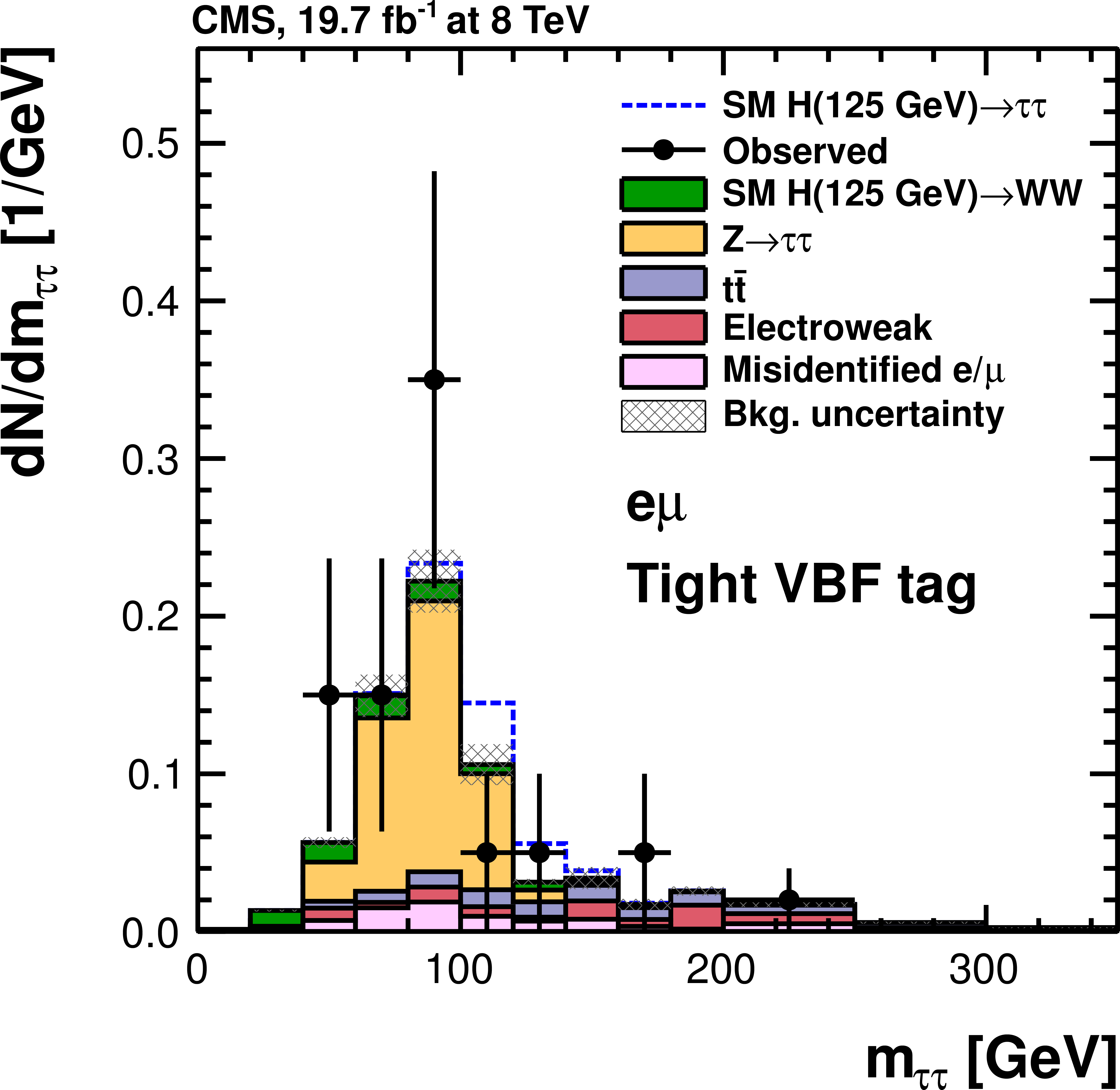
Figure 24-a:
Observed and predicted $ {m_{ {\tau } {\tau }}} $ distributions in the $ {\mathrm {e}} {{\mu }}$ channel, for all categories used in the 8 TeV data analysis. The normalization of the predicted background distributions corresponds to the result of the global fit. The signal distribution, on the other hand, is normalized to the SM prediction. The signal and background histograms are stacked. |

png pdf |
Figure 24-b:
Observed and predicted $ {m_{ {\tau } {\tau }}} $ distributions in the $ {\mathrm {e}} {{\mu }}$ channel, for all categories used in the 8 TeV data analysis. The normalization of the predicted background distributions corresponds to the result of the global fit. The signal distribution, on the other hand, is normalized to the SM prediction. The signal and background histograms are stacked. |
png pdf |
Figure 24-c:
Observed and predicted $ {m_{ {\tau } {\tau }}} $ distributions in the $ {\mathrm {e}} {{\mu }}$ channel, for all categories used in the 8 TeV data analysis. The normalization of the predicted background distributions corresponds to the result of the global fit. The signal distribution, on the other hand, is normalized to the SM prediction. The signal and background histograms are stacked. |

png pdf |
Figure 24-d:
Observed and predicted $ {m_{ {\tau } {\tau }}} $ distributions in the $ {\mathrm {e}} {{\mu }}$ channel, for all categories used in the 8 TeV data analysis. The normalization of the predicted background distributions corresponds to the result of the global fit. The signal distribution, on the other hand, is normalized to the SM prediction. The signal and background histograms are stacked. |

png pdf |
Figure 24-e:
Observed and predicted $ {m_{ {\tau } {\tau }}} $ distributions in the $ {\mathrm {e}} {{\mu }}$ channel, for all categories used in the 8 TeV data analysis. The normalization of the predicted background distributions corresponds to the result of the global fit. The signal distribution, on the other hand, is normalized to the SM prediction. The signal and background histograms are stacked. |

png pdf |
Figure 24-f:
Observed and predicted $ {m_{ {\tau } {\tau }}} $ distributions in the $ {\mathrm {e}} {{\mu }}$ channel, for all categories used in the 8 TeV data analysis. The normalization of the predicted background distributions corresponds to the result of the global fit. The signal distribution, on the other hand, is normalized to the SM prediction. The signal and background histograms are stacked. |
png pdf |
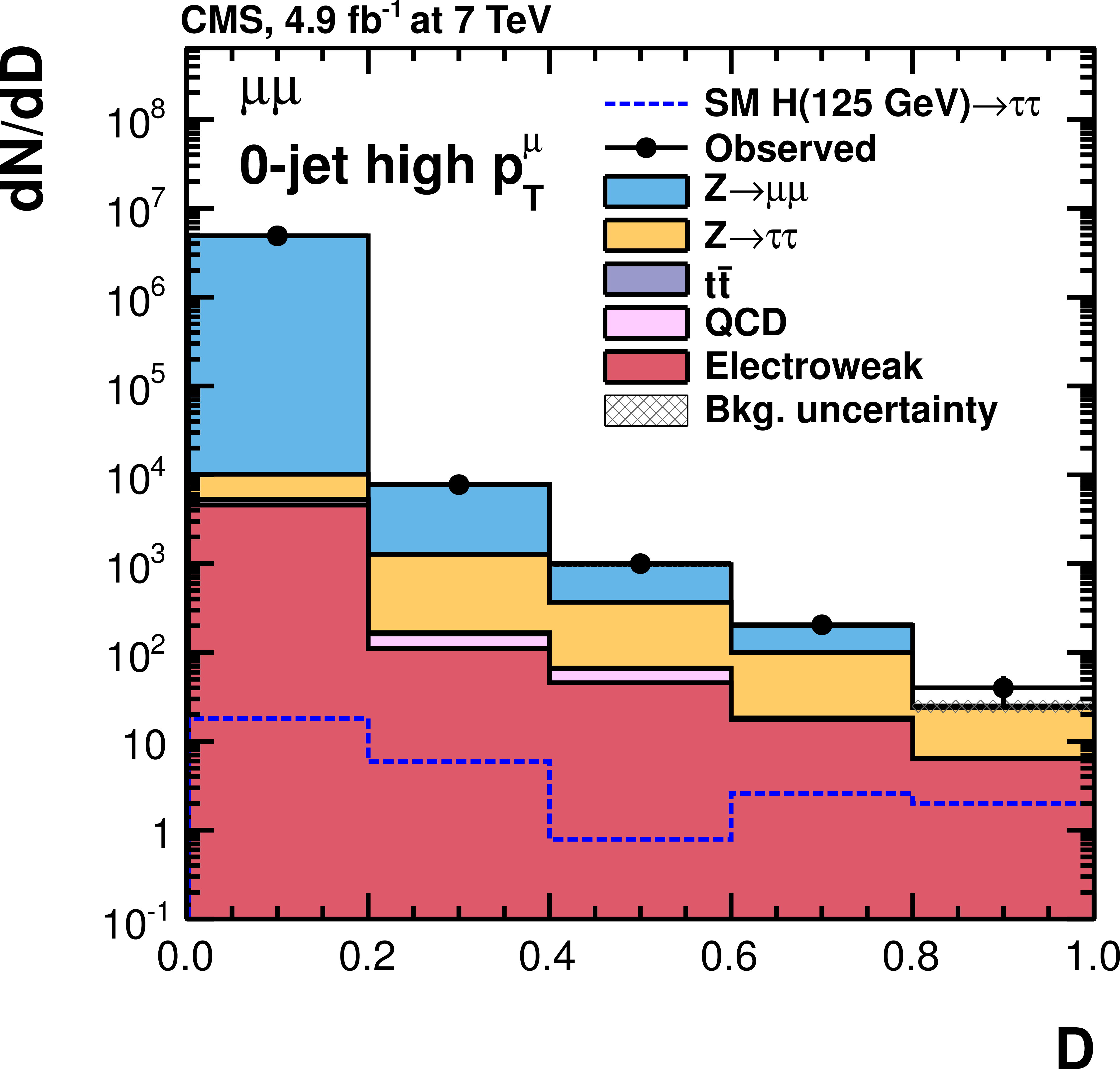
Figure 25-a:
Observed and predicted $D$ distributions in the $ {{\mu }} {{\mu }}$ channel, for all categories used in the 7 TeV data analysis. The normalization of the predicted background distributions corresponds to the result of the global fit. The signal distribution, on the other hand, is normalized to the SM prediction. The open signal histogram is shown superimposed to the background histograms, which are stacked. |
png pdf |
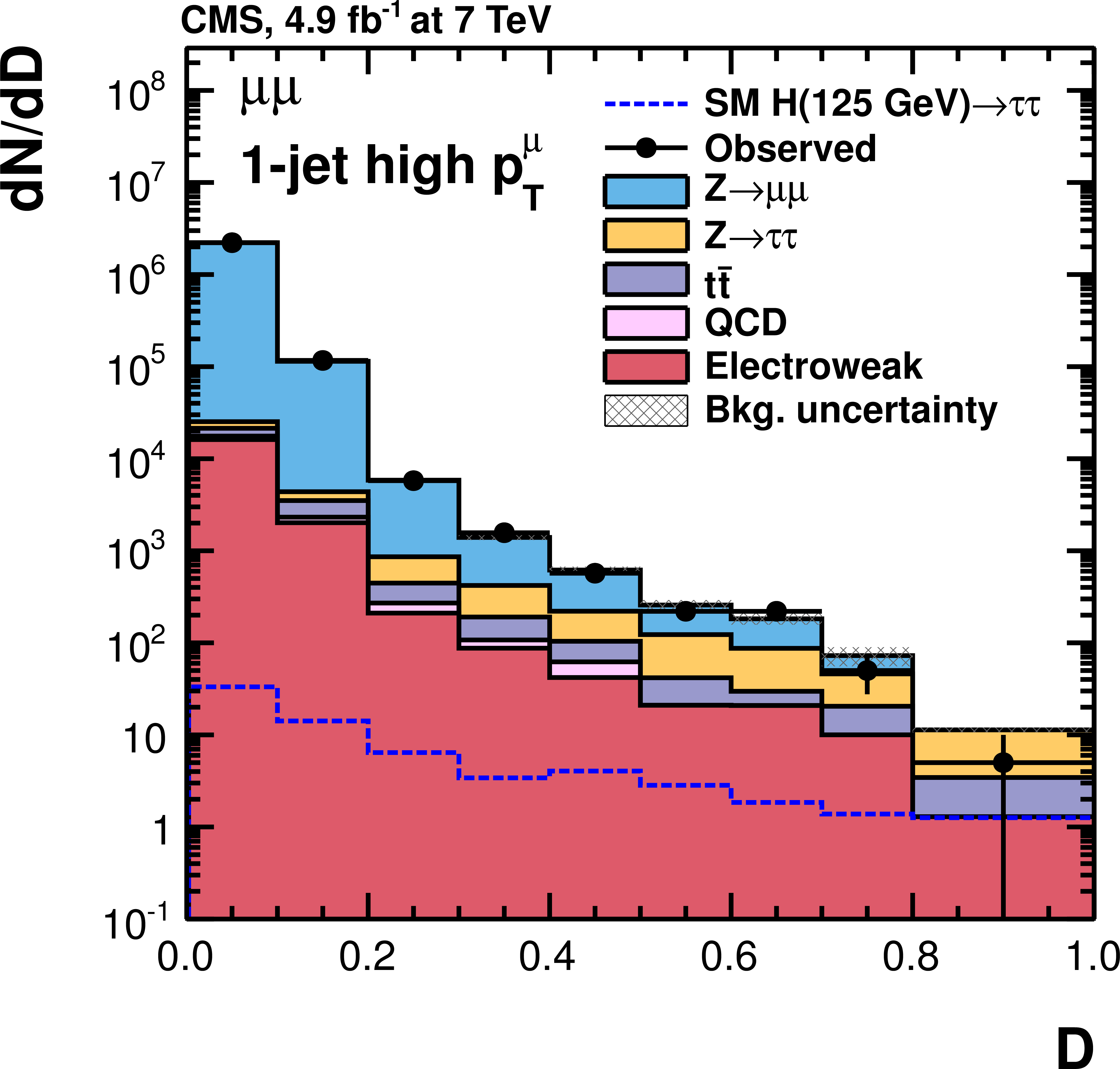
Figure 25-b:
Observed and predicted $D$ distributions in the $ {{\mu }} {{\mu }}$ channel, for all categories used in the 7 TeV data analysis. The normalization of the predicted background distributions corresponds to the result of the global fit. The signal distribution, on the other hand, is normalized to the SM prediction. The open signal histogram is shown superimposed to the background histograms, which are stacked. |

png pdf |
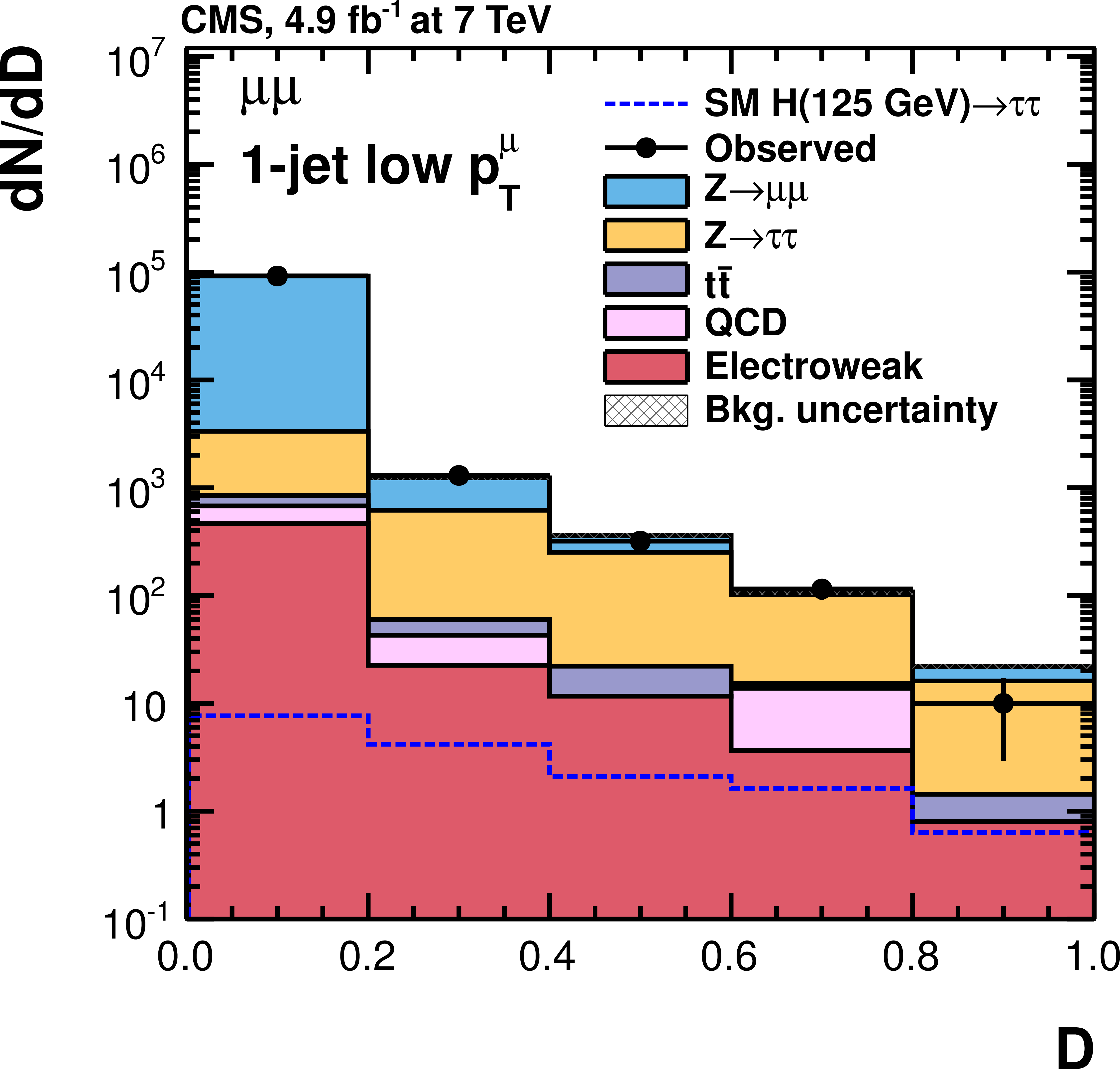
Figure 25-c:
Observed and predicted $D$ distributions in the $ {{\mu }} {{\mu }}$ channel, for all categories used in the 7 TeV data analysis. The normalization of the predicted background distributions corresponds to the result of the global fit. The signal distribution, on the other hand, is normalized to the SM prediction. The open signal histogram is shown superimposed to the background histograms, which are stacked. |
png pdf |
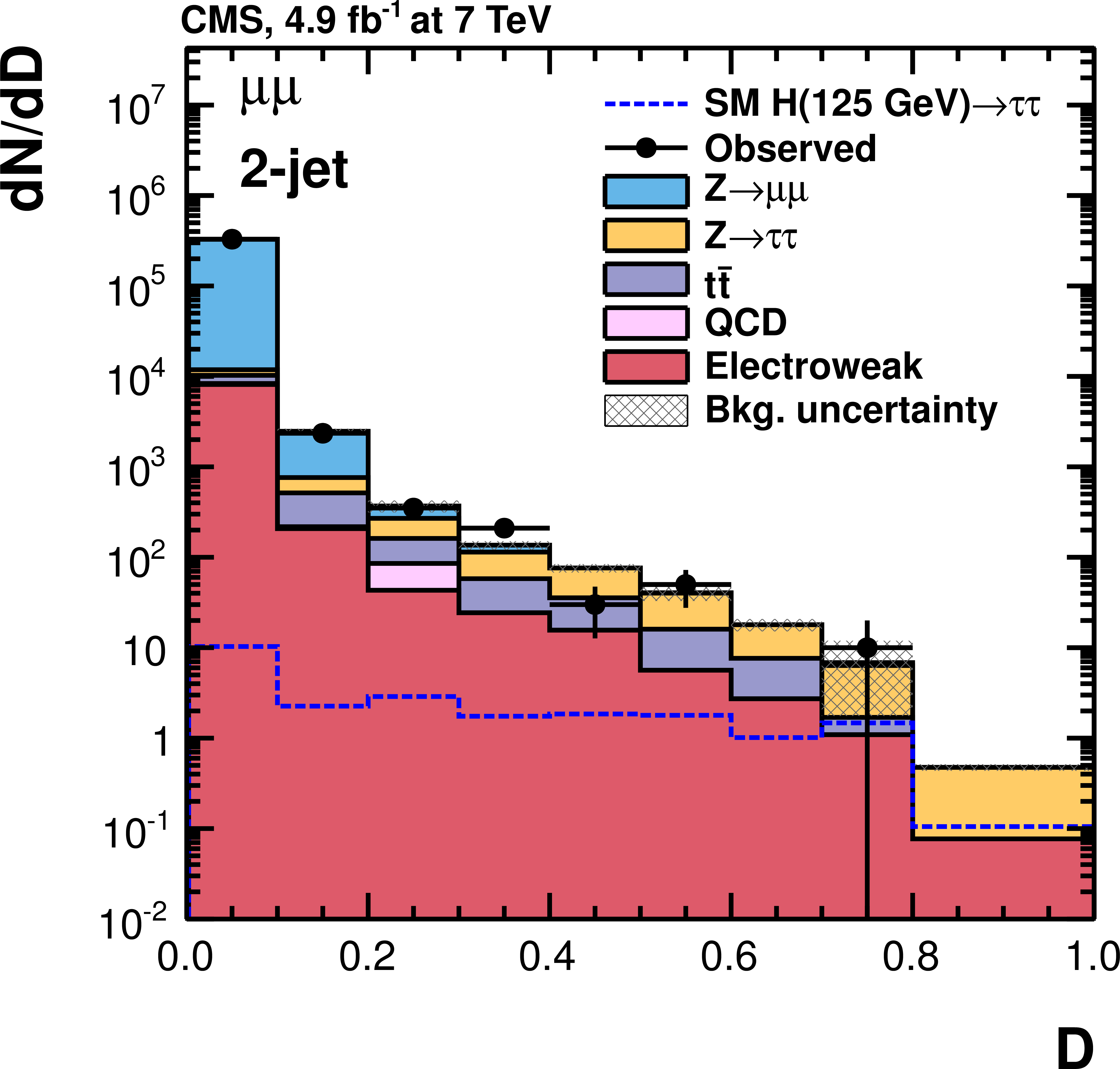
Figure 25-d:
Observed and predicted $D$ distributions in the $ {{\mu }} {{\mu }}$ channel, for all categories used in the 7 TeV data analysis. The normalization of the predicted background distributions corresponds to the result of the global fit. The signal distribution, on the other hand, is normalized to the SM prediction. The open signal histogram is shown superimposed to the background histograms, which are stacked. |
png pdf |
Figure 25-e:
Observed and predicted $D$ distributions in the $ {{\mu }} {{\mu }}$ channel, for all categories used in the 7 TeV data analysis. The normalization of the predicted background distributions corresponds to the result of the global fit. The signal distribution, on the other hand, is normalized to the SM prediction. The open signal histogram is shown superimposed to the background histograms, which are stacked. |

png pdf |
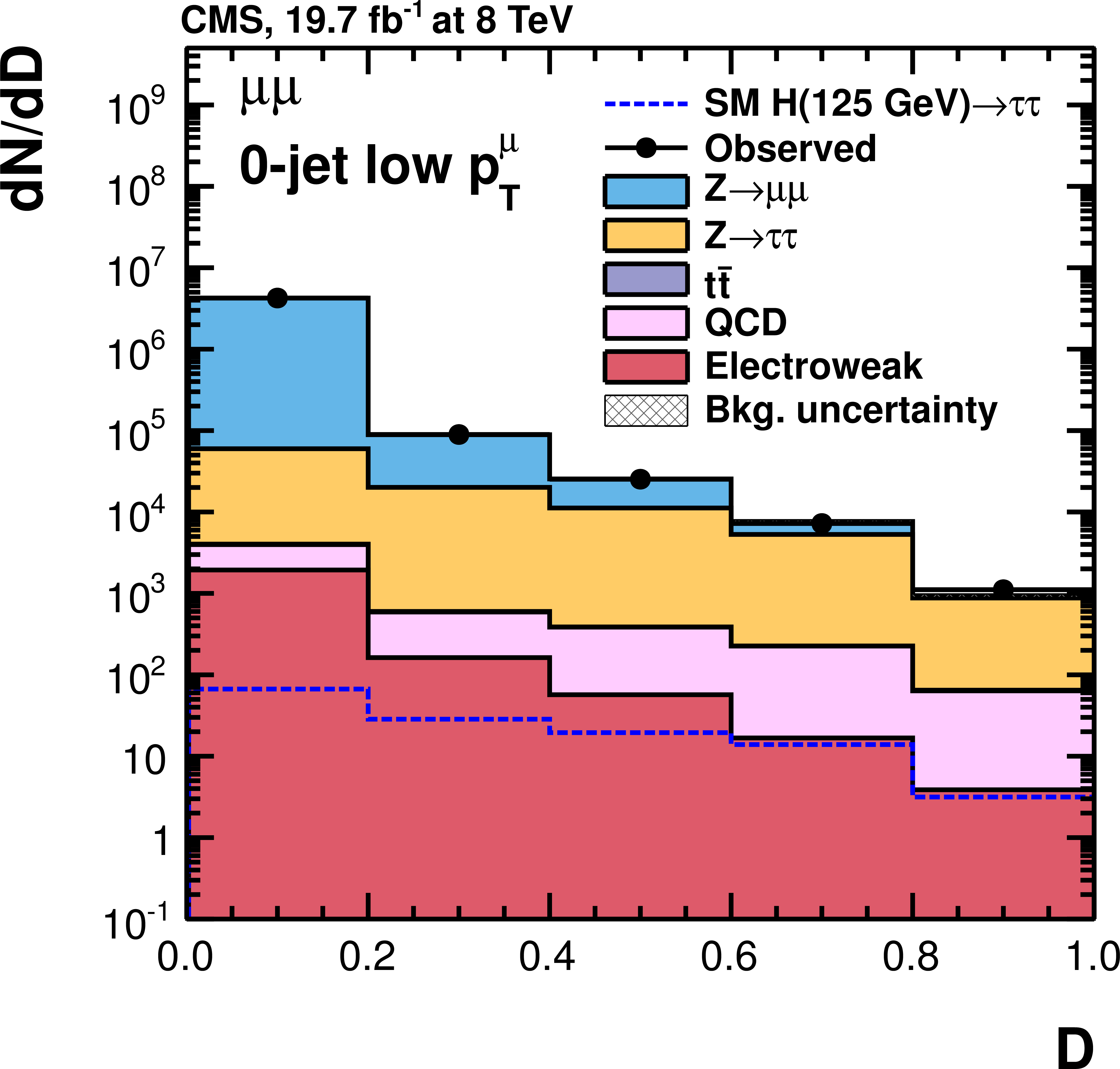
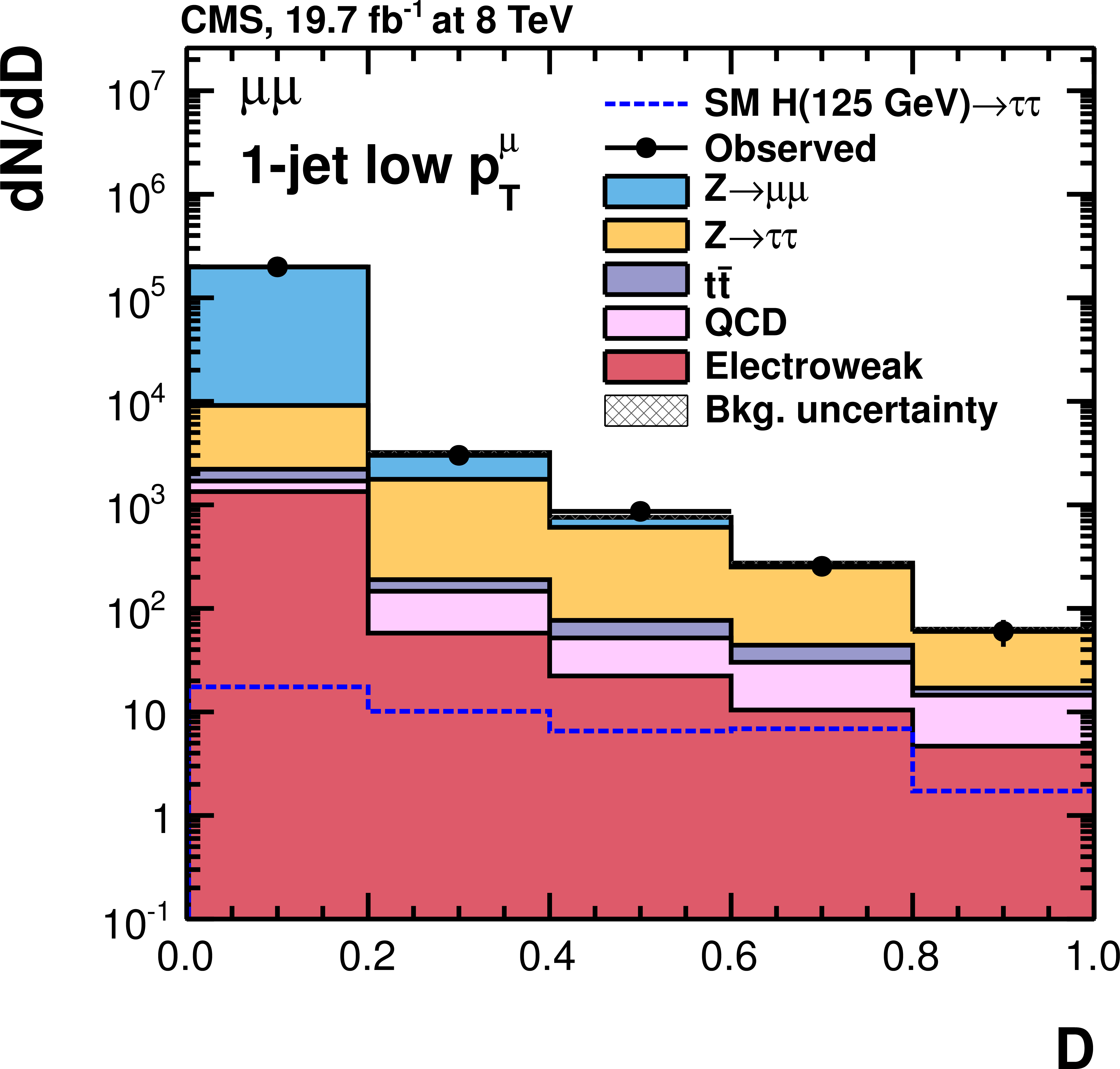
Figure 26-a:
Observed and predicted $D$ distributions in the $ {{\mu }} {{\mu }}$ channel, for all categories used in the 8 TeV data analysis. The normalization of the predicted background distributions corresponds to the result of the global fit. The signal distribution, on the other hand, is normalized to the SM prediction. The open signal histogram is shown superimposed to the background histograms, which are stacked. |
png pdf |
Figure 26-b:
Observed and predicted $D$ distributions in the $ {{\mu }} {{\mu }}$ channel, for all categories used in the 8 TeV data analysis. The normalization of the predicted background distributions corresponds to the result of the global fit. The signal distribution, on the other hand, is normalized to the SM prediction. The open signal histogram is shown superimposed to the background histograms, which are stacked. |
png pdf |
Figure 26-c:
Observed and predicted $D$ distributions in the $ {{\mu }} {{\mu }}$ channel, for all categories used in the 8 TeV data analysis. The normalization of the predicted background distributions corresponds to the result of the global fit. The signal distribution, on the other hand, is normalized to the SM prediction. The open signal histogram is shown superimposed to the background histograms, which are stacked. |
png pdf |
Figure 26-d:
Observed and predicted $D$ distributions in the $ {{\mu }} {{\mu }}$ channel, for all categories used in the 8 TeV data analysis. The normalization of the predicted background distributions corresponds to the result of the global fit. The signal distribution, on the other hand, is normalized to the SM prediction. The open signal histogram is shown superimposed to the background histograms, which are stacked. |

png pdf |
Figure 26-e:
Observed and predicted $D$ distributions in the $ {{\mu }} {{\mu }}$ channel, for all categories used in the 8 TeV data analysis. The normalization of the predicted background distributions corresponds to the result of the global fit. The signal distribution, on the other hand, is normalized to the SM prediction. The open signal histogram is shown superimposed to the background histograms, which are stacked. |
png pdf |
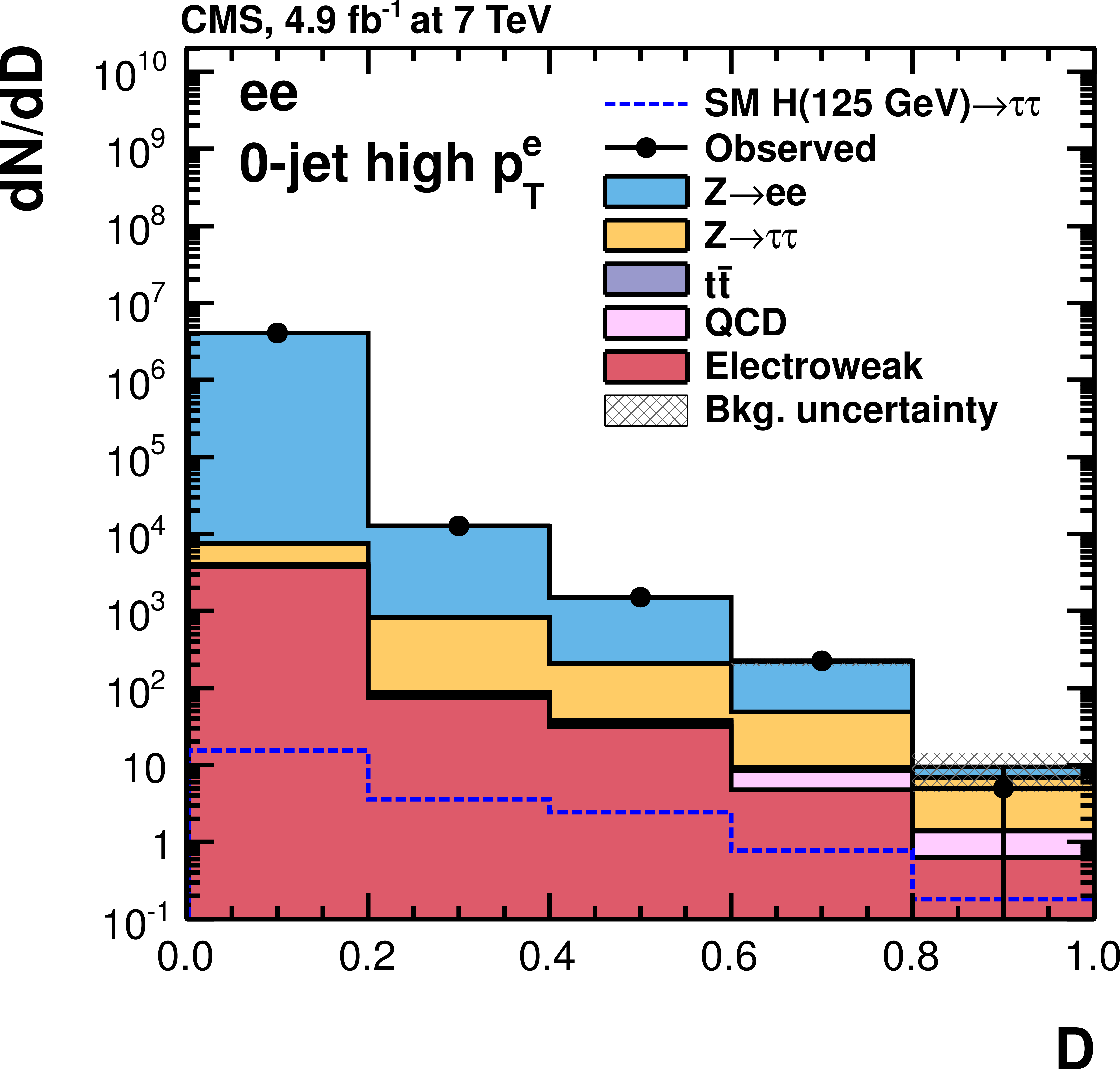
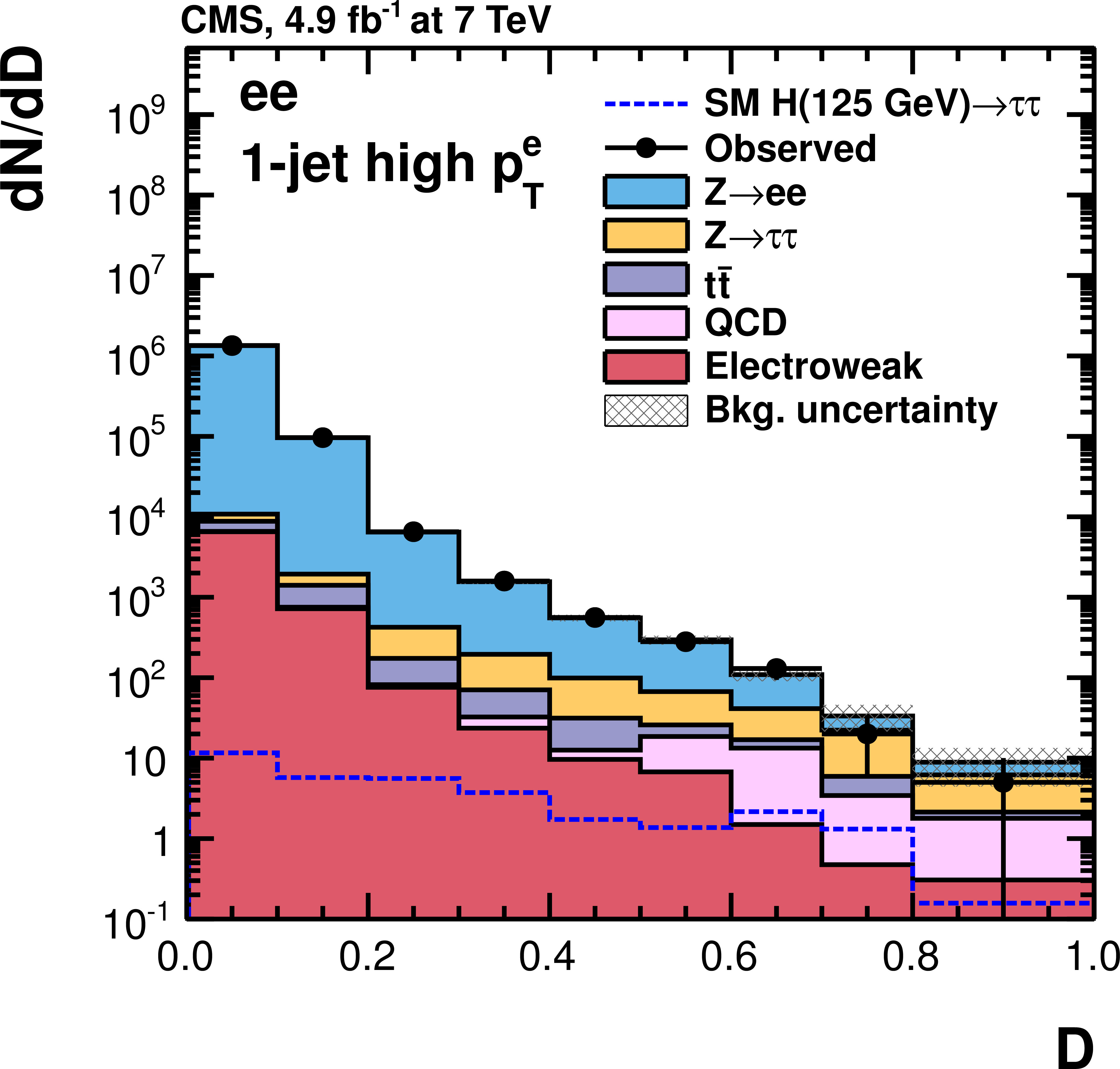
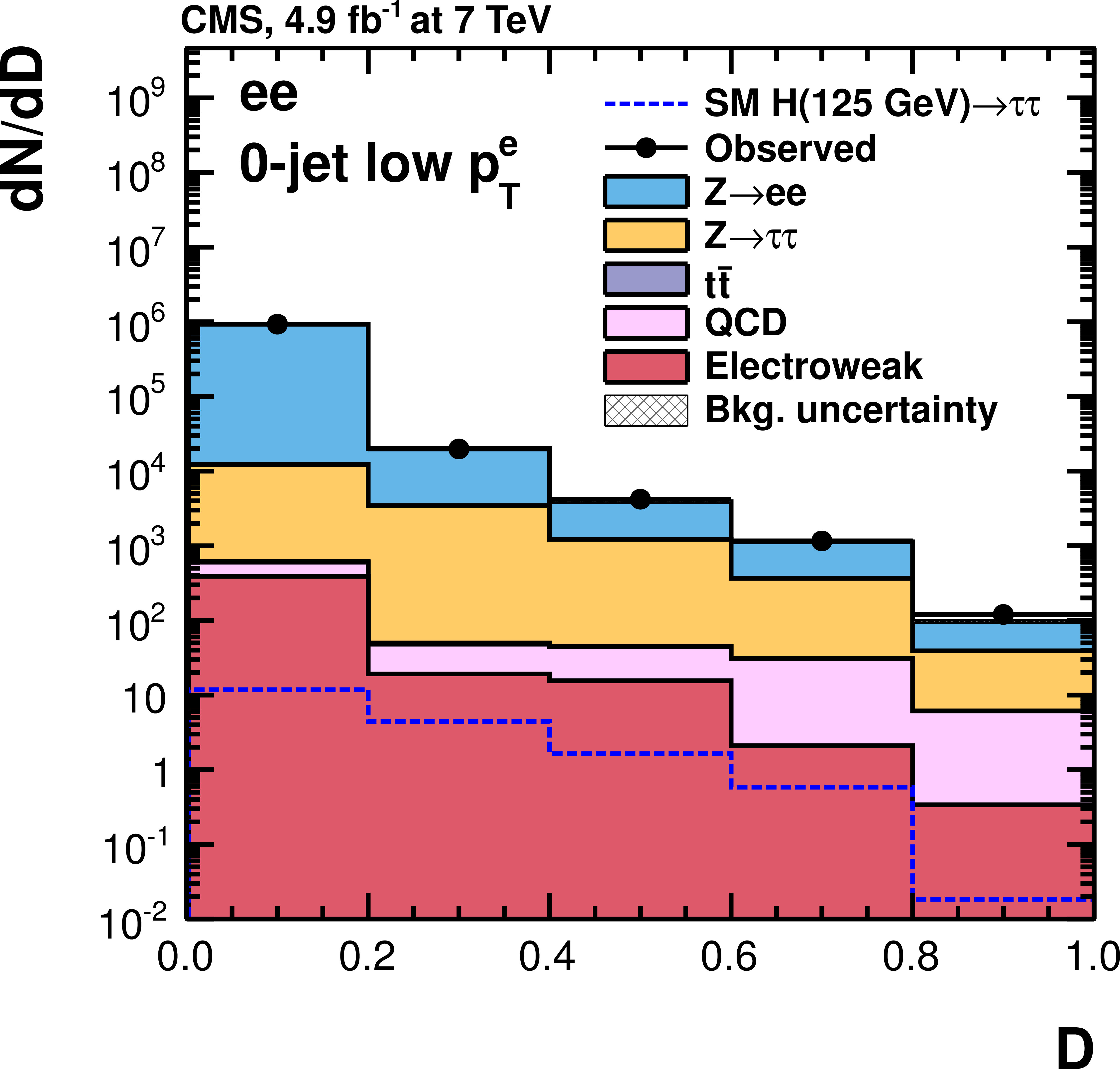
Figure 27-a:
Observed and predicted $D$ distributions in the $ {\mathrm {e}} {\mathrm {e}}$ channel, for all categories used in the 7 TeV data analysis. The normalization of the predicted background distributions corresponds to the result of the global fit. The signal distribution, on the other hand, is normalized to the SM prediction. The open signal histogram is shown superimposed to the background histograms, which are stacked. |
png pdf |
Figure 27-b:
Observed and predicted $D$ distributions in the $ {\mathrm {e}} {\mathrm {e}}$ channel, for all categories used in the 7 TeV data analysis. The normalization of the predicted background distributions corresponds to the result of the global fit. The signal distribution, on the other hand, is normalized to the SM prediction. The open signal histogram is shown superimposed to the background histograms, which are stacked. |
png pdf |
Figure 27-c:
Observed and predicted $D$ distributions in the $ {\mathrm {e}} {\mathrm {e}}$ channel, for all categories used in the 7 TeV data analysis. The normalization of the predicted background distributions corresponds to the result of the global fit. The signal distribution, on the other hand, is normalized to the SM prediction. The open signal histogram is shown superimposed to the background histograms, which are stacked. |

png pdf |
Figure 27-d:
Observed and predicted $D$ distributions in the $ {\mathrm {e}} {\mathrm {e}}$ channel, for all categories used in the 7 TeV data analysis. The normalization of the predicted background distributions corresponds to the result of the global fit. The signal distribution, on the other hand, is normalized to the SM prediction. The open signal histogram is shown superimposed to the background histograms, which are stacked. |

png pdf |
Figure 27-e:
Observed and predicted $D$ distributions in the $ {\mathrm {e}} {\mathrm {e}}$ channel, for all categories used in the 7 TeV data analysis. The normalization of the predicted background distributions corresponds to the result of the global fit. The signal distribution, on the other hand, is normalized to the SM prediction. The open signal histogram is shown superimposed to the background histograms, which are stacked. |

png pdf |
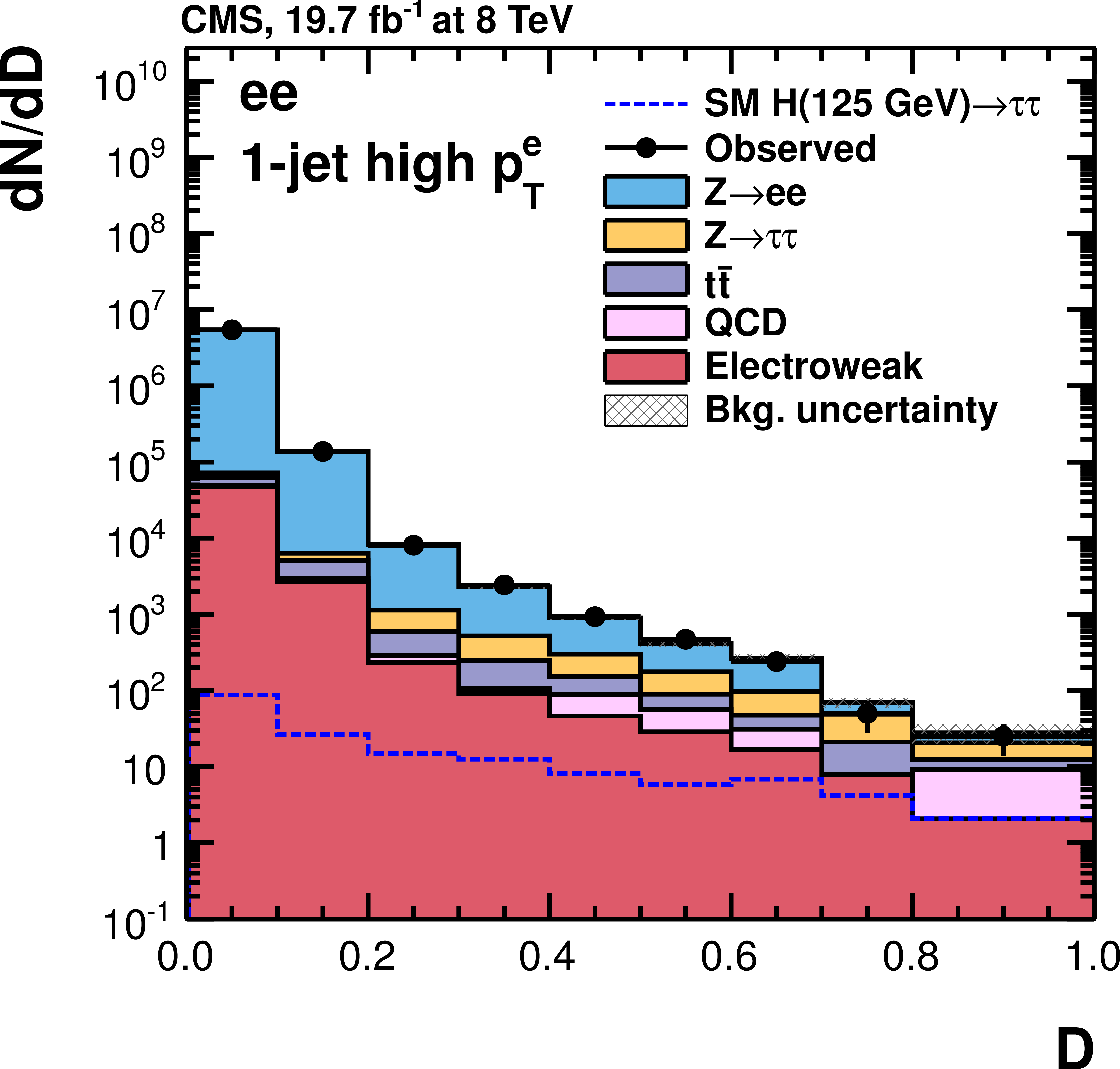
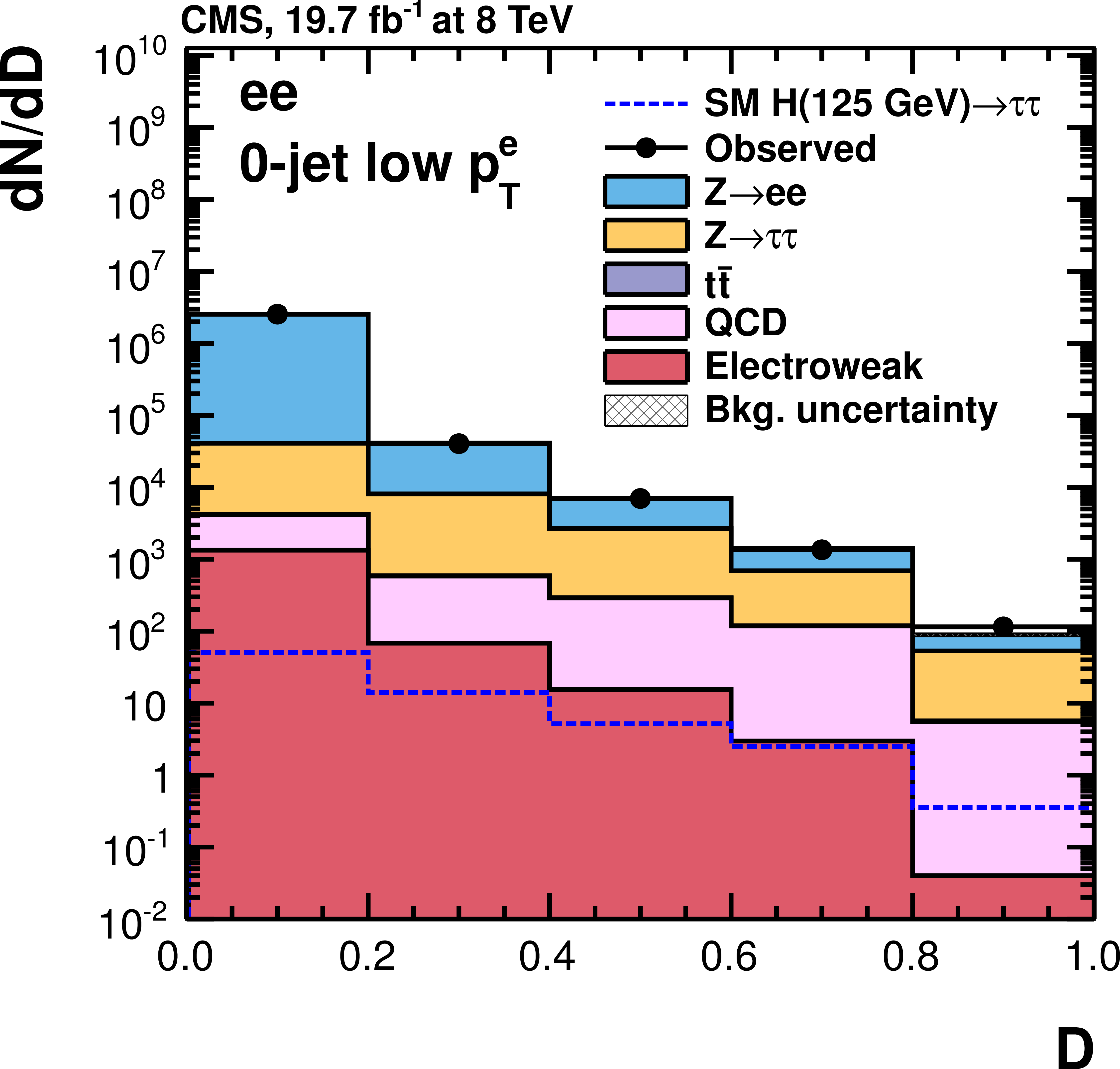
Figure 28-a:
Observed and predicted $D$ distributions in the $ {\mathrm {e}} {\mathrm {e}}$ channel, for all categories used in the 8 TeV data analysis. The normalization of the predicted background distributions corresponds to the result of the global fit. The signal distribution, on the other hand, is normalized to the SM prediction. The open signal histogram is shown superimposed to the background histograms, which are stacked. |
png pdf |
Figure 28-b:
Observed and predicted $D$ distributions in the $ {\mathrm {e}} {\mathrm {e}}$ channel, for all categories used in the 8 TeV data analysis. The normalization of the predicted background distributions corresponds to the result of the global fit. The signal distribution, on the other hand, is normalized to the SM prediction. The open signal histogram is shown superimposed to the background histograms, which are stacked. |
png pdf |
Figure 28-c:
Observed and predicted $D$ distributions in the $ {\mathrm {e}} {\mathrm {e}}$ channel, for all categories used in the 8 TeV data analysis. The normalization of the predicted background distributions corresponds to the result of the global fit. The signal distribution, on the other hand, is normalized to the SM prediction. The open signal histogram is shown superimposed to the background histograms, which are stacked. |
png pdf |
Figure 28-d:
Observed and predicted $D$ distributions in the $ {\mathrm {e}} {\mathrm {e}}$ channel, for all categories used in the 8 TeV data analysis. The normalization of the predicted background distributions corresponds to the result of the global fit. The signal distribution, on the other hand, is normalized to the SM prediction. The open signal histogram is shown superimposed to the background histograms, which are stacked. |

png pdf |
Figure 28-e:
Observed and predicted $D$ distributions in the $ {\mathrm {e}} {\mathrm {e}}$ channel, for all categories used in the 8 TeV data analysis. The normalization of the predicted background distributions corresponds to the result of the global fit. The signal distribution, on the other hand, is normalized to the SM prediction. The open signal histogram is shown superimposed to the background histograms, which are stacked. |
png pdf |
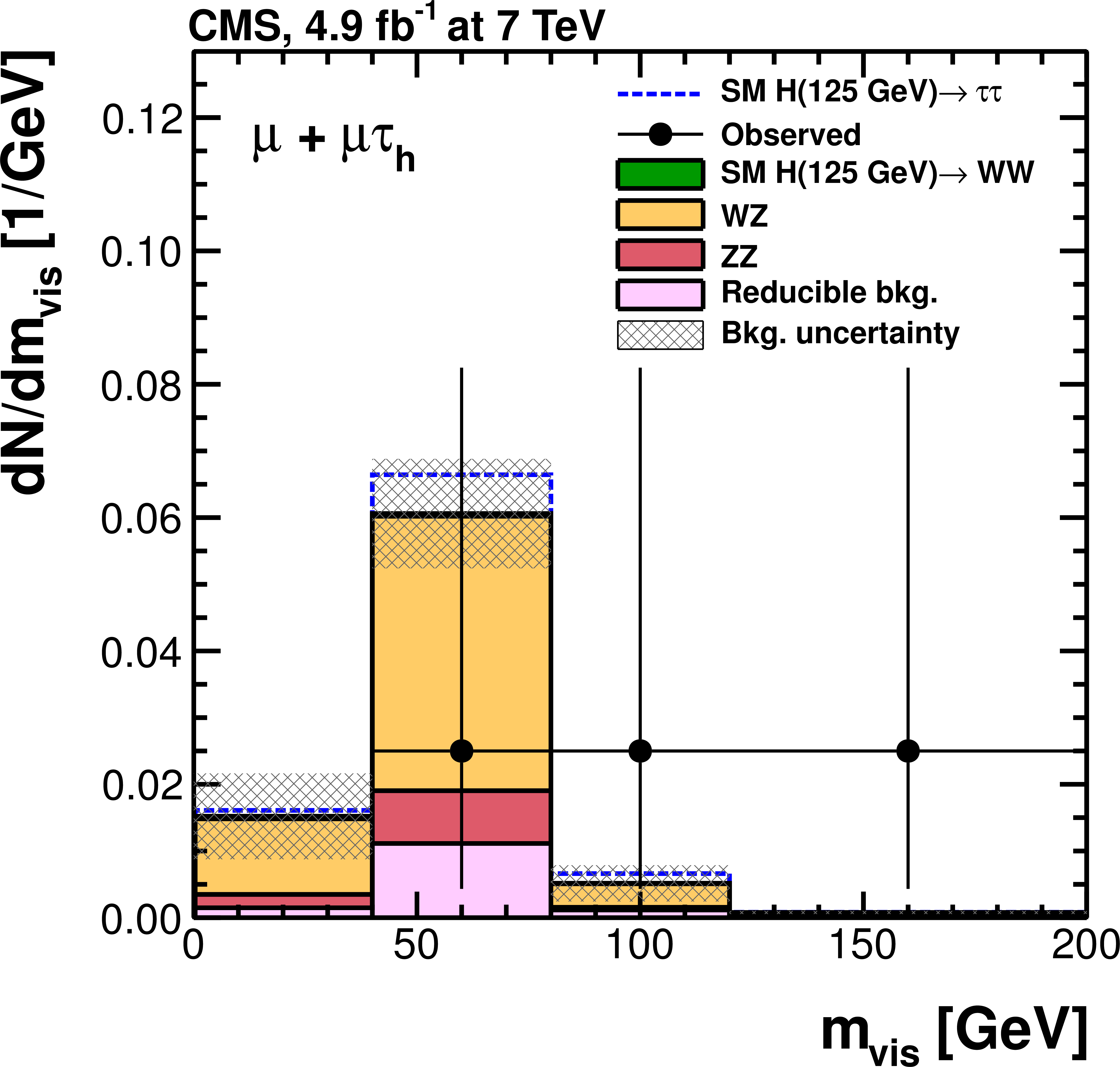
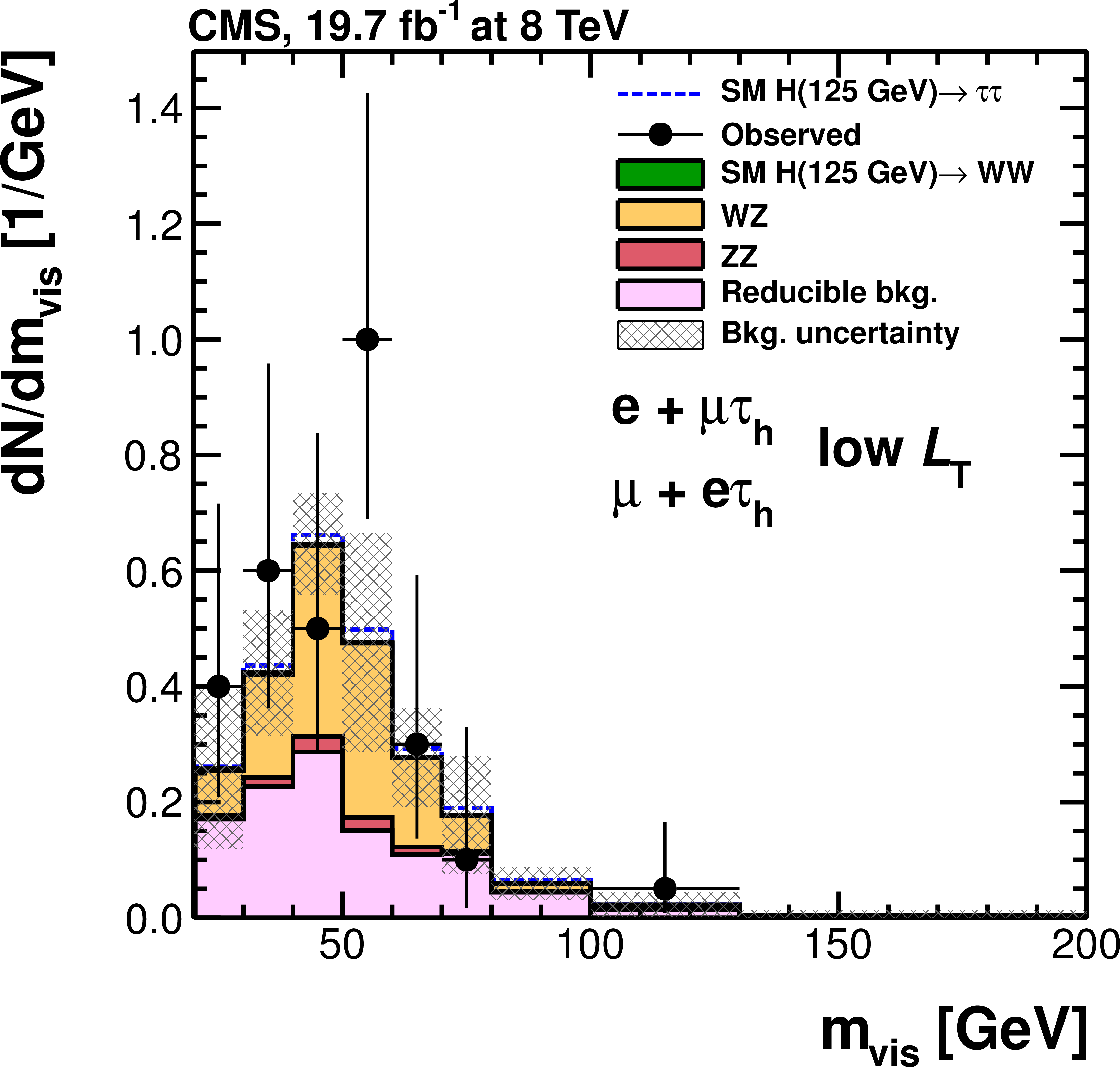
Figure 29-a:
Observed and predicted $ {m_\text {vis}} $ distributions in the $ {{\mu }}+ {{\mu }} { {\tau }_{\rm h}} $ (a, c, e) and $ {\mathrm {e}}+ {{\mu }} { {\tau }_{\rm h}} / {{\mu }}+ {\mathrm {e}} { {\tau }_{\rm h}} $ (b, d, f) channels for the 7 TeV data analysis (a, b) and in the low-$ {L_\mathrm {T}} $ (c, d) and high-$ {L_\mathrm {T}} $ (e, f) categories used in the 8 TeV data analysis. The normalization of the predicted background distributions corresponds to the result of the global fit. The signal distribution, on the other hand, is normalized to the SM prediction. The signal and background histograms are stacked. |
png pdf |
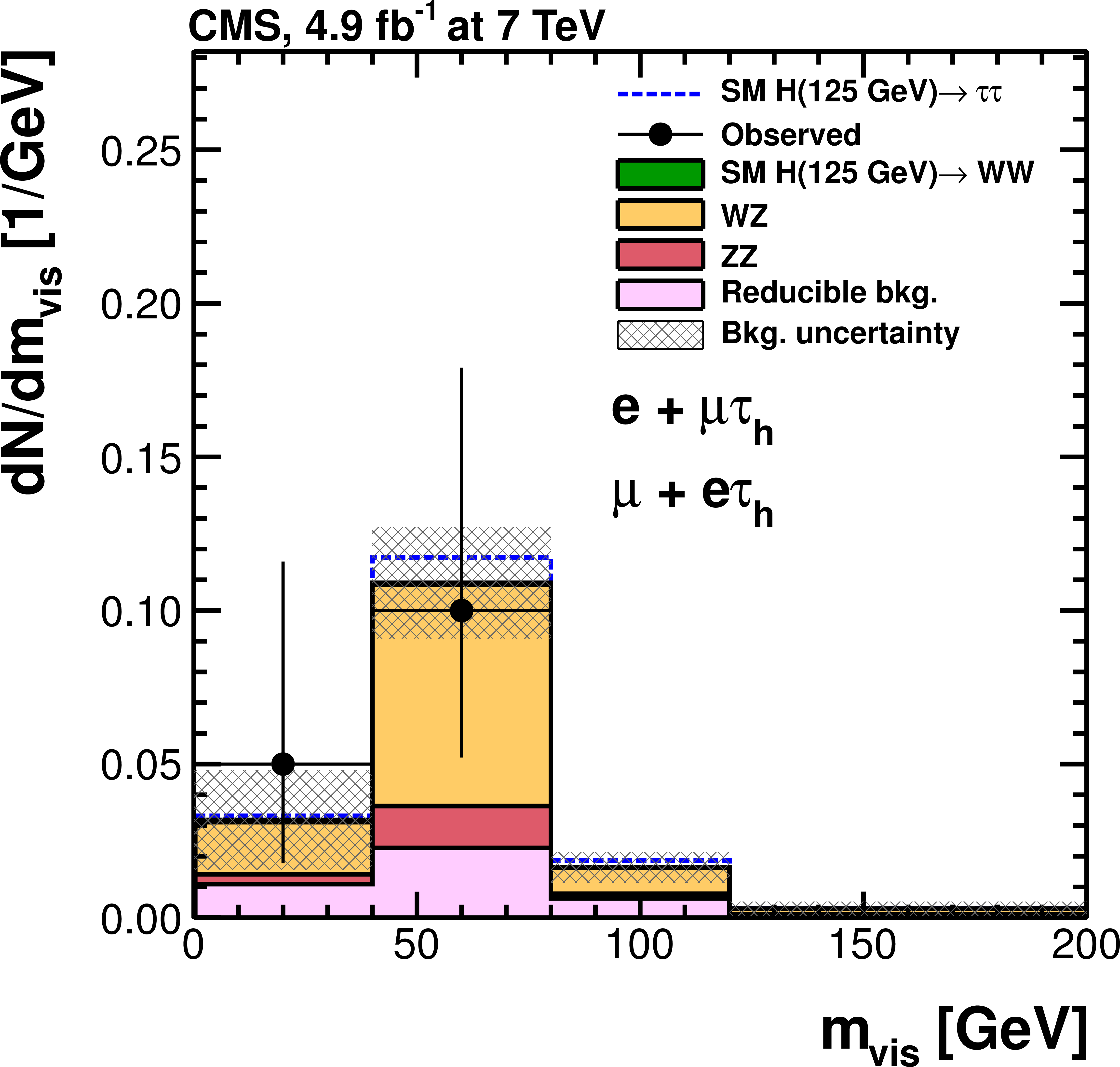
Figure 29-b:
Observed and predicted $ {m_\text {vis}} $ distributions in the $ {{\mu }}+ {{\mu }} { {\tau }_{\rm h}} $ (a, c, e) and $ {\mathrm {e}}+ {{\mu }} { {\tau }_{\rm h}} / {{\mu }}+ {\mathrm {e}} { {\tau }_{\rm h}} $ (b, d, f) channels for the 7 TeV data analysis (a, b) and in the low-$ {L_\mathrm {T}} $ (c, d) and high-$ {L_\mathrm {T}} $ (e, f) categories used in the 8 TeV data analysis. The normalization of the predicted background distributions corresponds to the result of the global fit. The signal distribution, on the other hand, is normalized to the SM prediction. The signal and background histograms are stacked. |
png pdf |
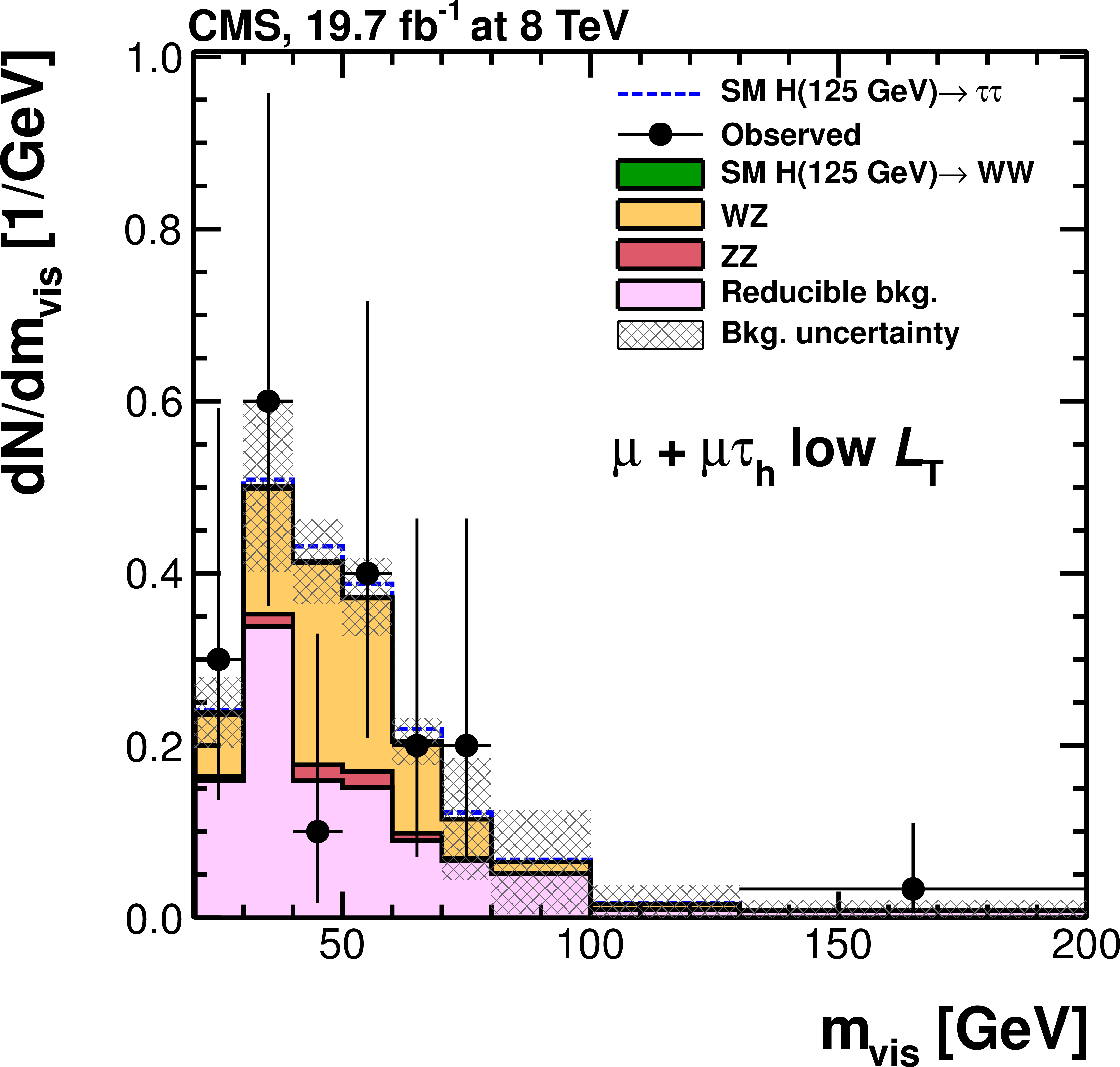
Figure 29-c:
Observed and predicted $ {m_\text {vis}} $ distributions in the $ {{\mu }}+ {{\mu }} { {\tau }_{\rm h}} $ (a, c, e) and $ {\mathrm {e}}+ {{\mu }} { {\tau }_{\rm h}} / {{\mu }}+ {\mathrm {e}} { {\tau }_{\rm h}} $ (b, d, f) channels for the 7 TeV data analysis (a, b) and in the low-$ {L_\mathrm {T}} $ (c, d) and high-$ {L_\mathrm {T}} $ (e, f) categories used in the 8 TeV data analysis. The normalization of the predicted background distributions corresponds to the result of the global fit. The signal distribution, on the other hand, is normalized to the SM prediction. The signal and background histograms are stacked. |
png pdf |
Figure 29-d:
Observed and predicted $ {m_\text {vis}} $ distributions in the $ {{\mu }}+ {{\mu }} { {\tau }_{\rm h}} $ (a, c, e) and $ {\mathrm {e}}+ {{\mu }} { {\tau }_{\rm h}} / {{\mu }}+ {\mathrm {e}} { {\tau }_{\rm h}} $ (b, d, f) channels for the 7 TeV data analysis (a, b) and in the low-$ {L_\mathrm {T}} $ (c, d) and high-$ {L_\mathrm {T}} $ (e, f) categories used in the 8 TeV data analysis. The normalization of the predicted background distributions corresponds to the result of the global fit. The signal distribution, on the other hand, is normalized to the SM prediction. The signal and background histograms are stacked. |

png pdf |
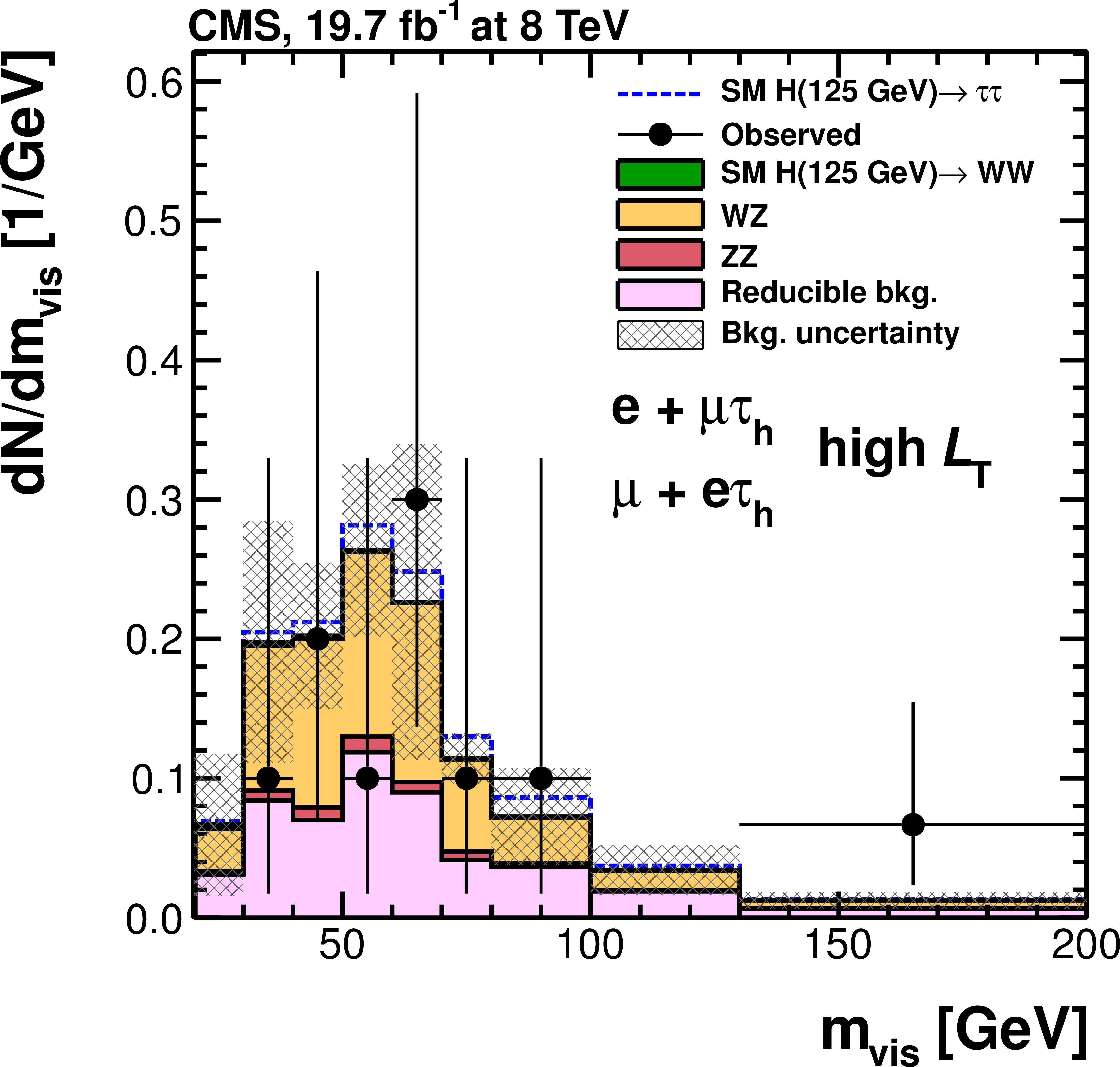
Figure 29-e:
Observed and predicted $ {m_\text {vis}} $ distributions in the $ {{\mu }}+ {{\mu }} { {\tau }_{\rm h}} $ (a, c, e) and $ {\mathrm {e}}+ {{\mu }} { {\tau }_{\rm h}} / {{\mu }}+ {\mathrm {e}} { {\tau }_{\rm h}} $ (b, d, f) channels for the 7 TeV data analysis (a, b) and in the low-$ {L_\mathrm {T}} $ (c, d) and high-$ {L_\mathrm {T}} $ (e, f) categories used in the 8 TeV data analysis. The normalization of the predicted background distributions corresponds to the result of the global fit. The signal distribution, on the other hand, is normalized to the SM prediction. The signal and background histograms are stacked. |
png pdf |
Figure 29-f:
Observed and predicted $ {m_\text {vis}} $ distributions in the $ {{\mu }}+ {{\mu }} { {\tau }_{\rm h}} $ (a, c, e) and $ {\mathrm {e}}+ {{\mu }} { {\tau }_{\rm h}} / {{\mu }}+ {\mathrm {e}} { {\tau }_{\rm h}} $ (b, d, f) channels for the 7 TeV data analysis (a, b) and in the low-$ {L_\mathrm {T}} $ (c, d) and high-$ {L_\mathrm {T}} $ (e, f) categories used in the 8 TeV data analysis. The normalization of the predicted background distributions corresponds to the result of the global fit. The signal distribution, on the other hand, is normalized to the SM prediction. The signal and background histograms are stacked. |
png pdf |
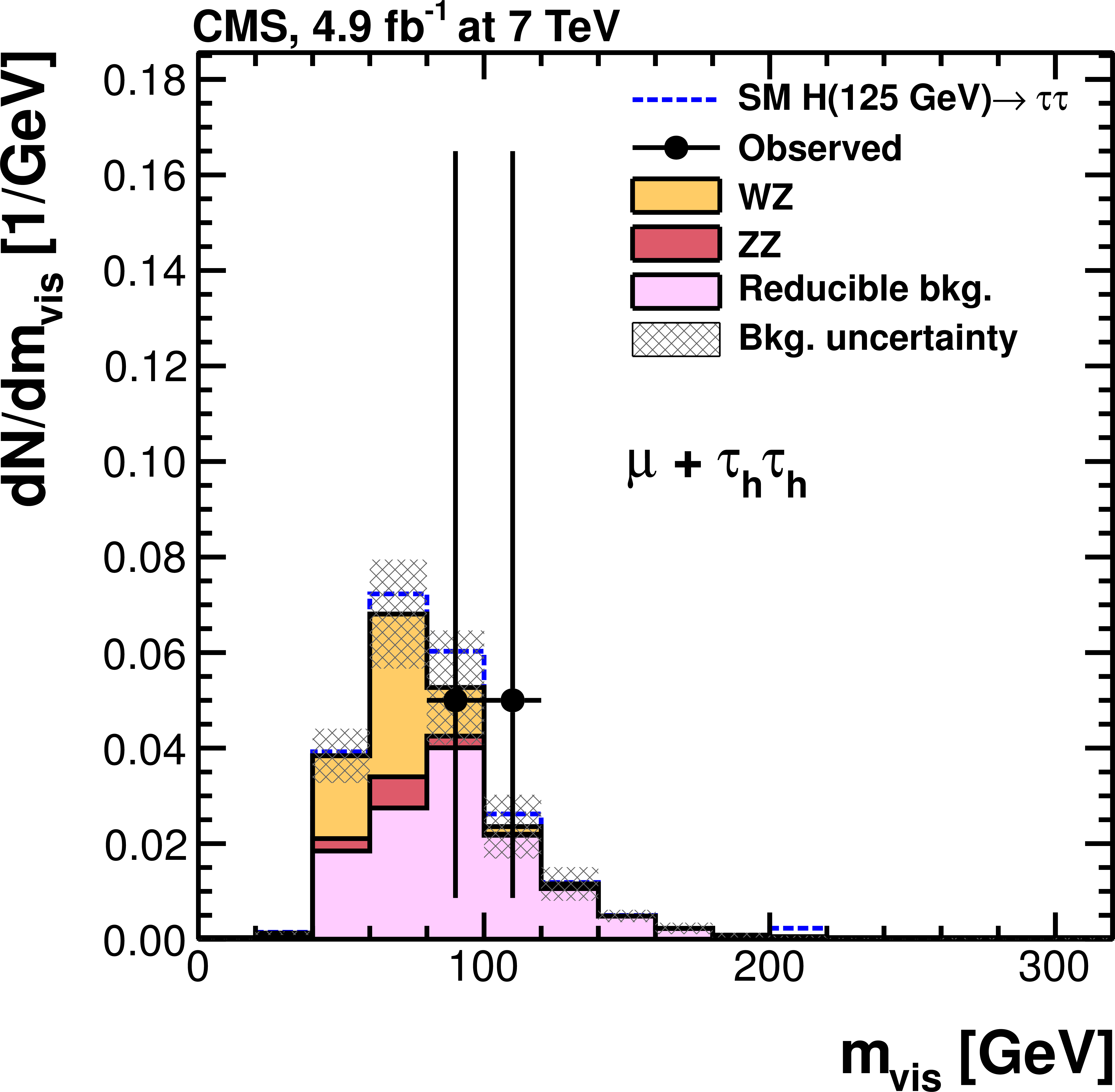
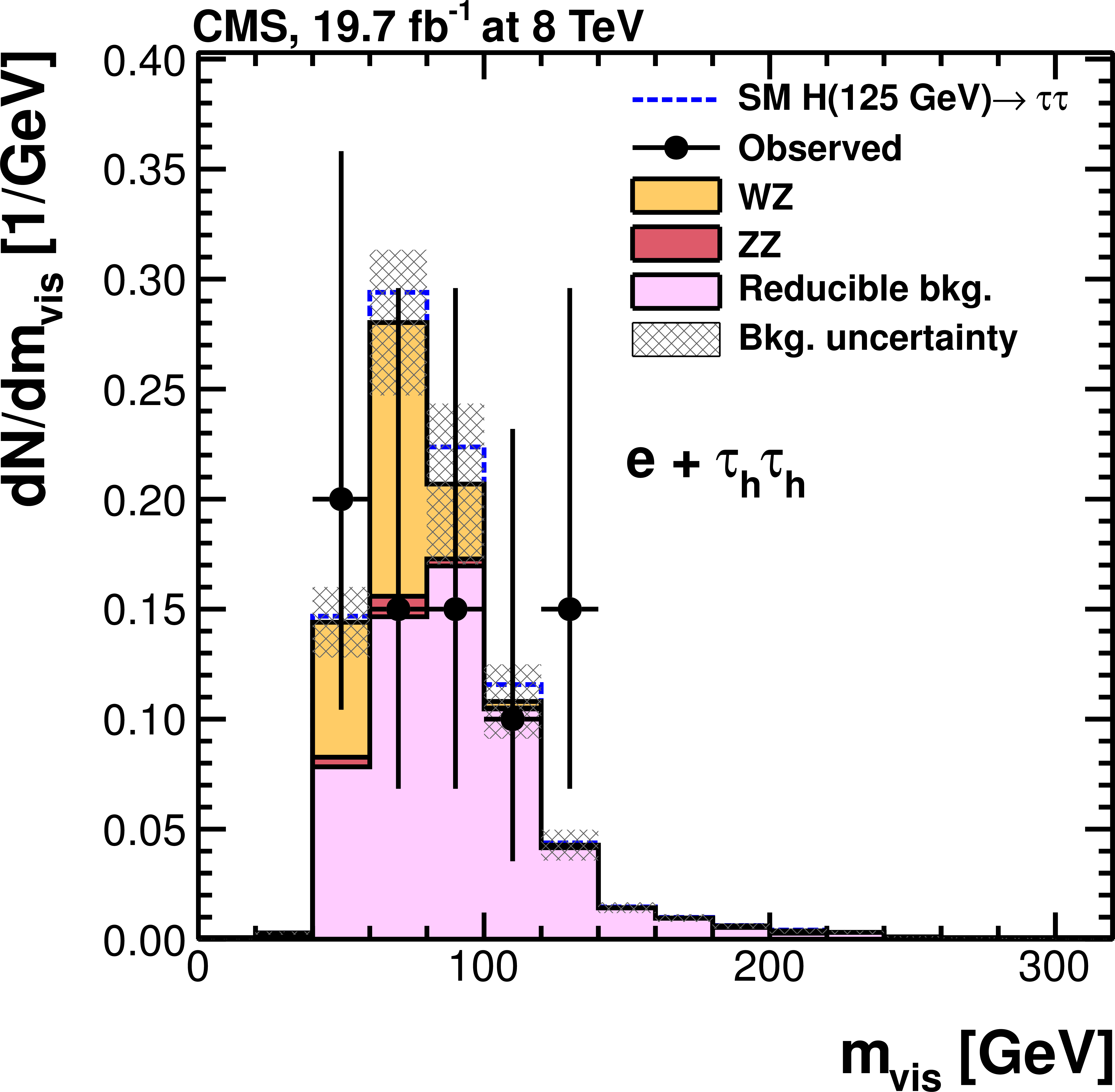
Figure 30-a:
Observed and predicted $ {m_\text {vis}} $ distributions in the $ {{\mu }}+ { {\tau }_{\rm h}} { {\tau }_{\rm h}} $ (a, c) and $ {\mathrm {e}}+ { {\tau }_{\rm h}} { {\tau }_{\rm h}} $ (b, d) channels for the 7 TeV data analysis (a, b) and the 8 TeV data analysis (c, d). The normalization of the predicted background distributions corresponds to the result of the global fit. The signal distribution, on the other hand, is normalized to the SM prediction. The signal and background histograms are stacked. |

png pdf |
Figure 30-b:
Observed and predicted $ {m_\text {vis}} $ distributions in the $ {{\mu }}+ { {\tau }_{\rm h}} { {\tau }_{\rm h}} $ (a, c) and $ {\mathrm {e}}+ { {\tau }_{\rm h}} { {\tau }_{\rm h}} $ (b, d) channels for the 7 TeV data analysis (a, b) and the 8 TeV data analysis (c, d). The normalization of the predicted background distributions corresponds to the result of the global fit. The signal distribution, on the other hand, is normalized to the SM prediction. The signal and background histograms are stacked. |
png pdf |
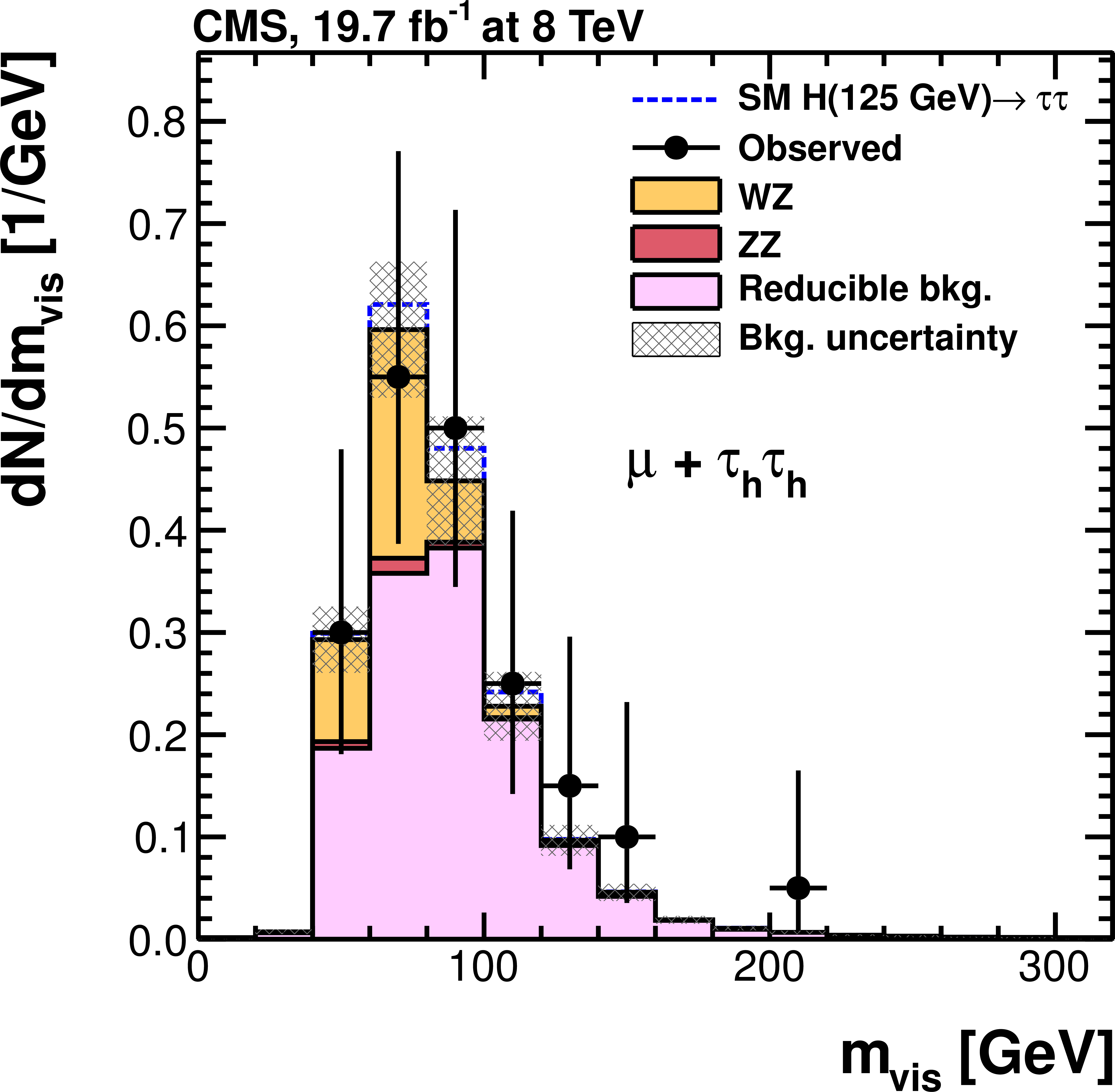
Figure 30-c:
Observed and predicted $ {m_\text {vis}} $ distributions in the $ {{\mu }}+ { {\tau }_{\rm h}} { {\tau }_{\rm h}} $ (a, c) and $ {\mathrm {e}}+ { {\tau }_{\rm h}} { {\tau }_{\rm h}} $ (b, d) channels for the 7 TeV data analysis (a, b) and the 8 TeV data analysis (c, d). The normalization of the predicted background distributions corresponds to the result of the global fit. The signal distribution, on the other hand, is normalized to the SM prediction. The signal and background histograms are stacked. |
png pdf |
Figure 30-d:
Observed and predicted $ {m_\text {vis}} $ distributions in the $ {{\mu }}+ { {\tau }_{\rm h}} { {\tau }_{\rm h}} $ (a, c) and $ {\mathrm {e}}+ { {\tau }_{\rm h}} { {\tau }_{\rm h}} $ (b, d) channels for the 7 TeV data analysis (a, b) and the 8 TeV data analysis (c, d). The normalization of the predicted background distributions corresponds to the result of the global fit. The signal distribution, on the other hand, is normalized to the SM prediction. The signal and background histograms are stacked. |

png pdf |
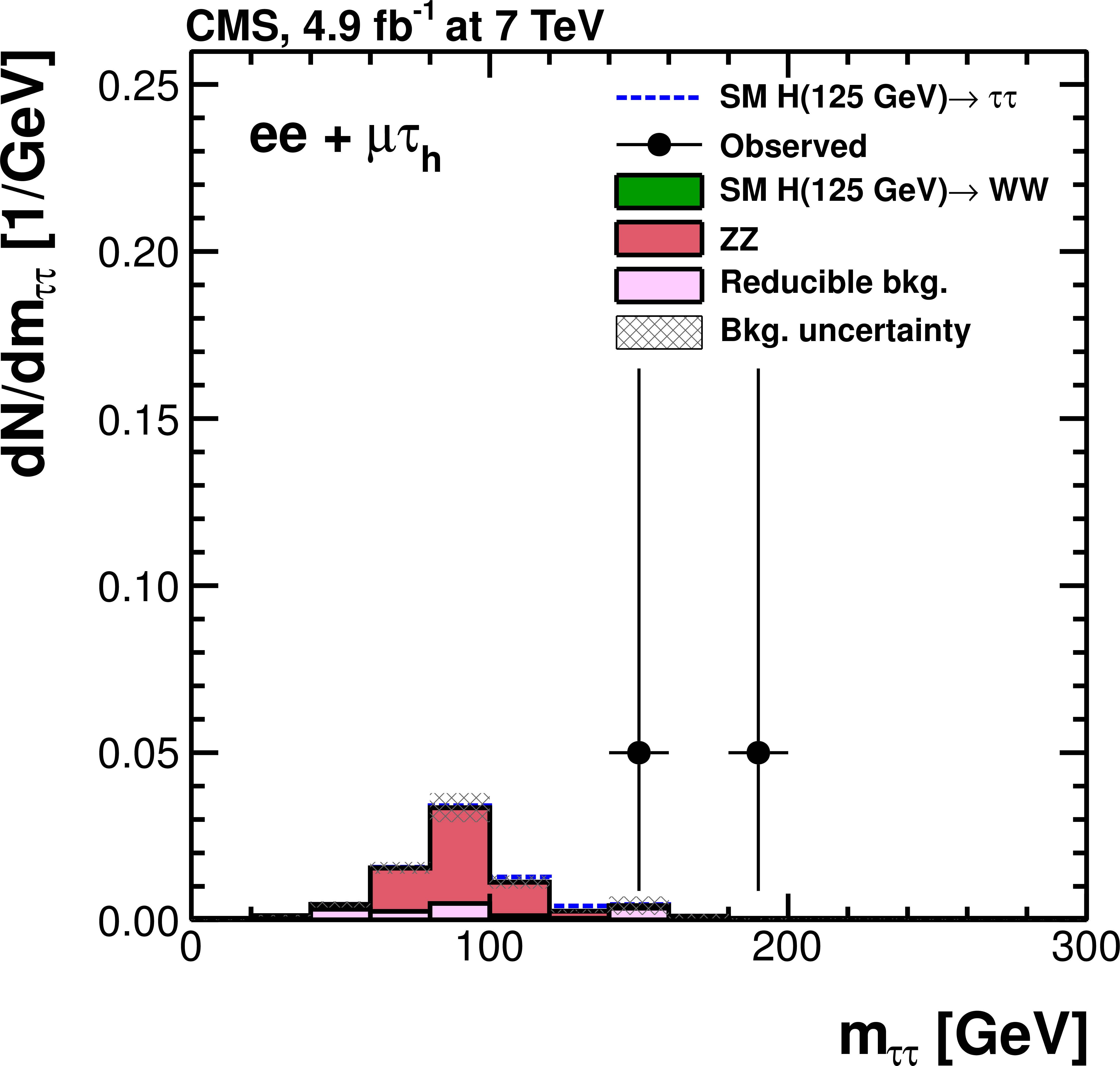
Figure 31-a:
Observed and predicted $ {m_{ {\tau } {\tau }}} $ distributions for the four different $LL'$ final states of the $ {\mathrm {e}} {\mathrm {e}}+ LL'$ (a) and $ {{\mu }} {{\mu }}+ LL'$ (b) channels for the 7 TeV data analysis. The normalization of the predicted background distributions corresponds to the result of the global fit. The signal distribution, on the other hand, is normalized to the SM prediction. The signal and background histograms are stacked. |
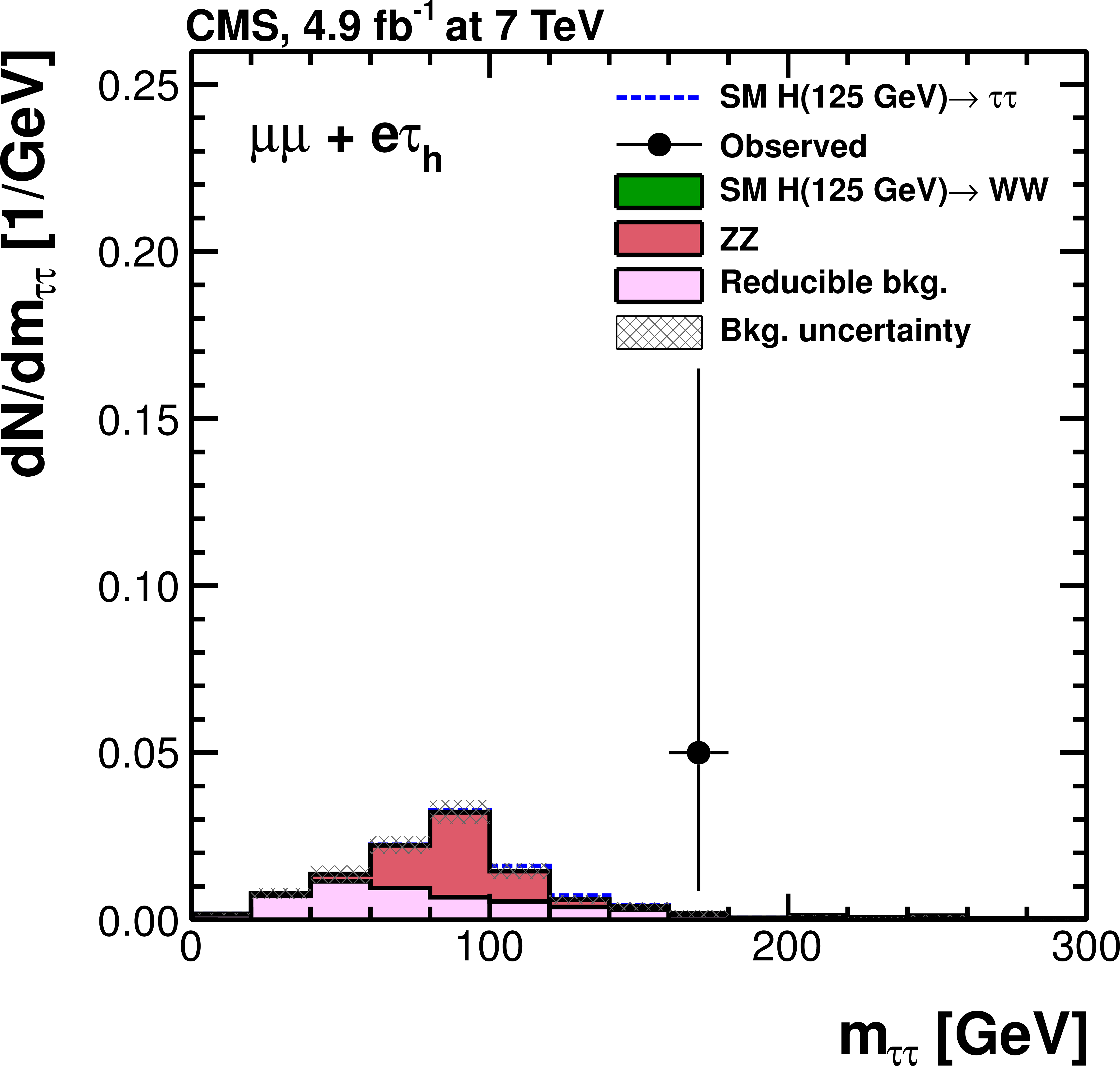
png pdf |
Figure 31-b:
Observed and predicted $ {m_{ {\tau } {\tau }}} $ distributions for the four different $LL'$ final states of the $ {\mathrm {e}} {\mathrm {e}}+ LL'$ (a) and $ {{\mu }} {{\mu }}+ LL'$ (b) channels for the 7 TeV data analysis. The normalization of the predicted background distributions corresponds to the result of the global fit. The signal distribution, on the other hand, is normalized to the SM prediction. The signal and background histograms are stacked. |
png pdf |
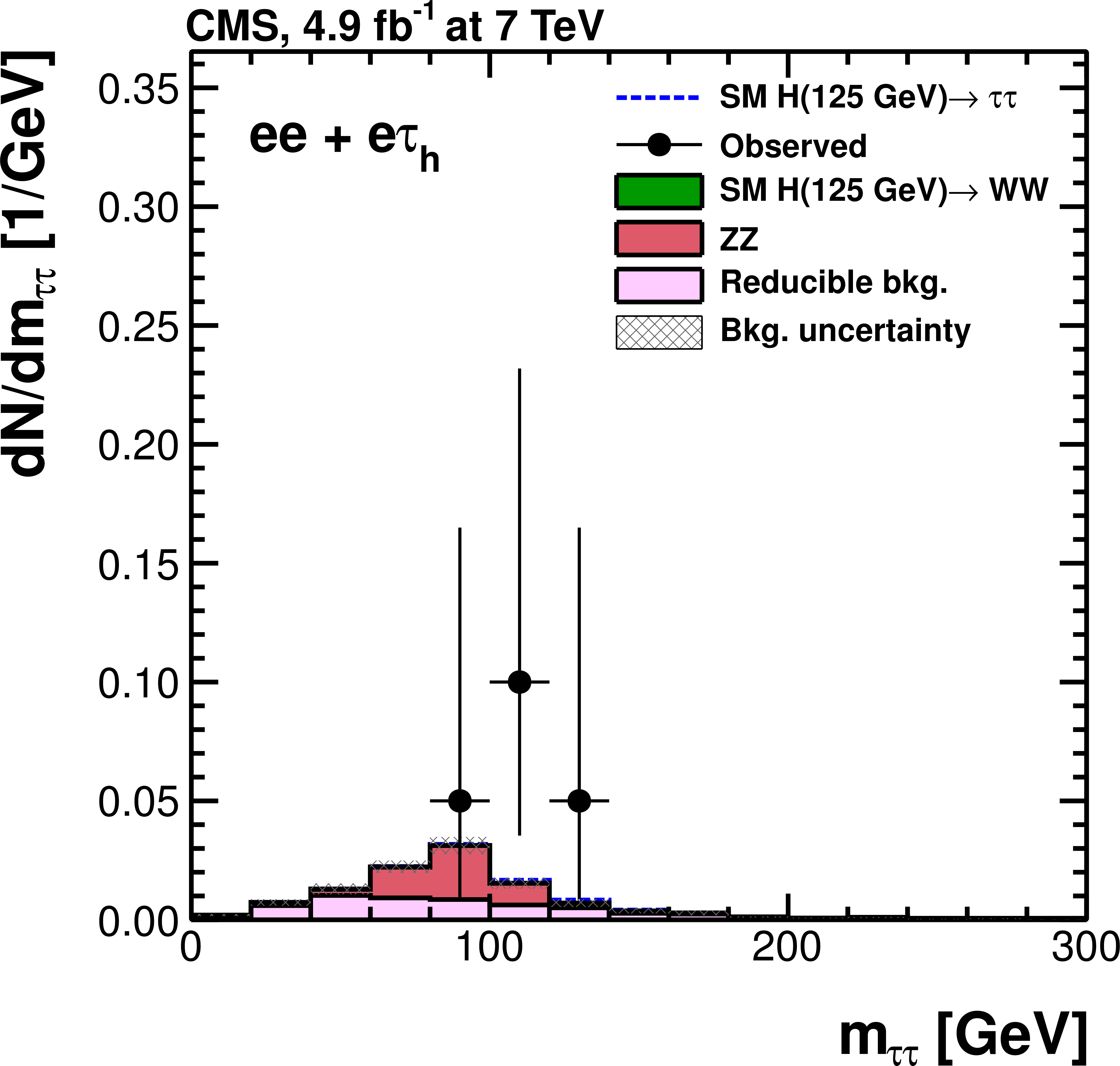
Figure 31-c:
Observed and predicted $ {m_{ {\tau } {\tau }}} $ distributions for the four different $LL'$ final states of the $ {\mathrm {e}} {\mathrm {e}}+ LL'$ (a) and $ {{\mu }} {{\mu }}+ LL'$ (b) channels for the 7 TeV data analysis. The normalization of the predicted background distributions corresponds to the result of the global fit. The signal distribution, on the other hand, is normalized to the SM prediction. The signal and background histograms are stacked. |
png pdf |
Figure 31-d:
Observed and predicted $ {m_{ {\tau } {\tau }}} $ distributions for the four different $LL'$ final states of the $ {\mathrm {e}} {\mathrm {e}}+ LL'$ (a) and $ {{\mu }} {{\mu }}+ LL'$ (b) channels for the 7 TeV data analysis. The normalization of the predicted background distributions corresponds to the result of the global fit. The signal distribution, on the other hand, is normalized to the SM prediction. The signal and background histograms are stacked. |
png pdf |
Figure 31-e:
Observed and predicted $ {m_{ {\tau } {\tau }}} $ distributions for the four different $LL'$ final states of the $ {\mathrm {e}} {\mathrm {e}}+ LL'$ (a) and $ {{\mu }} {{\mu }}+ LL'$ (b) channels for the 7 TeV data analysis. The normalization of the predicted background distributions corresponds to the result of the global fit. The signal distribution, on the other hand, is normalized to the SM prediction. The signal and background histograms are stacked. |
png pdf |
Figure 31-f:
Observed and predicted $ {m_{ {\tau } {\tau }}} $ distributions for the four different $LL'$ final states of the $ {\mathrm {e}} {\mathrm {e}}+ LL'$ (a) and $ {{\mu }} {{\mu }}+ LL'$ (b) channels for the 7 TeV data analysis. The normalization of the predicted background distributions corresponds to the result of the global fit. The signal distribution, on the other hand, is normalized to the SM prediction. The signal and background histograms are stacked. |
png pdf |
Figure 31-g:
Observed and predicted $ {m_{ {\tau } {\tau }}} $ distributions for the four different $LL'$ final states of the $ {\mathrm {e}} {\mathrm {e}}+ LL'$ (a) and $ {{\mu }} {{\mu }}+ LL'$ (b) channels for the 7 TeV data analysis. The normalization of the predicted background distributions corresponds to the result of the global fit. The signal distribution, on the other hand, is normalized to the SM prediction. The signal and background histograms are stacked. |
png pdf |
Figure 31-h:
Observed and predicted $ {m_{ {\tau } {\tau }}} $ distributions for the four different $LL'$ final states of the $ {\mathrm {e}} {\mathrm {e}}+ LL'$ (a) and $ {{\mu }} {{\mu }}+ LL'$ (b) channels for the 7 TeV data analysis. The normalization of the predicted background distributions corresponds to the result of the global fit. The signal distribution, on the other hand, is normalized to the SM prediction. The signal and background histograms are stacked. |
png pdf |
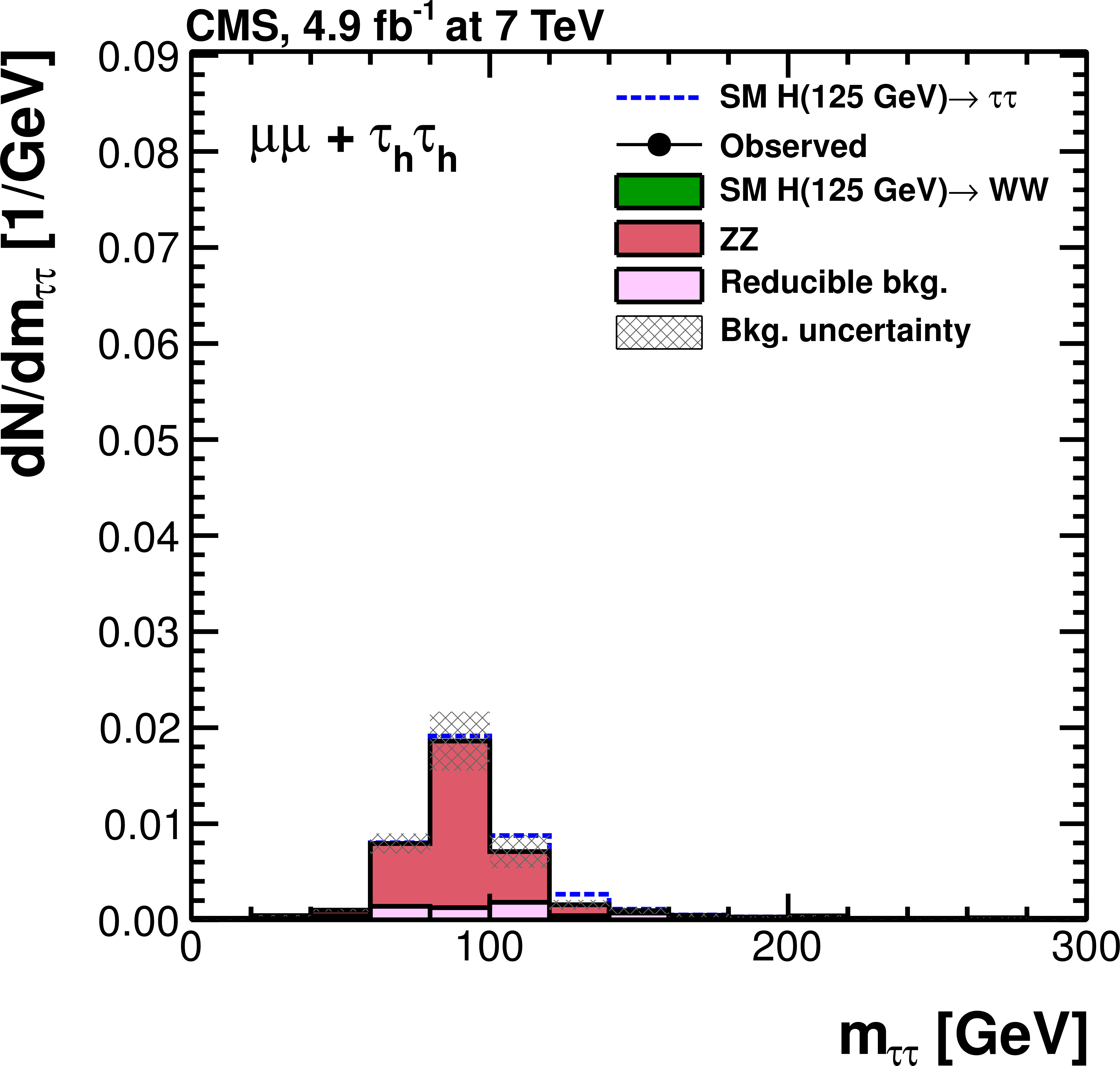
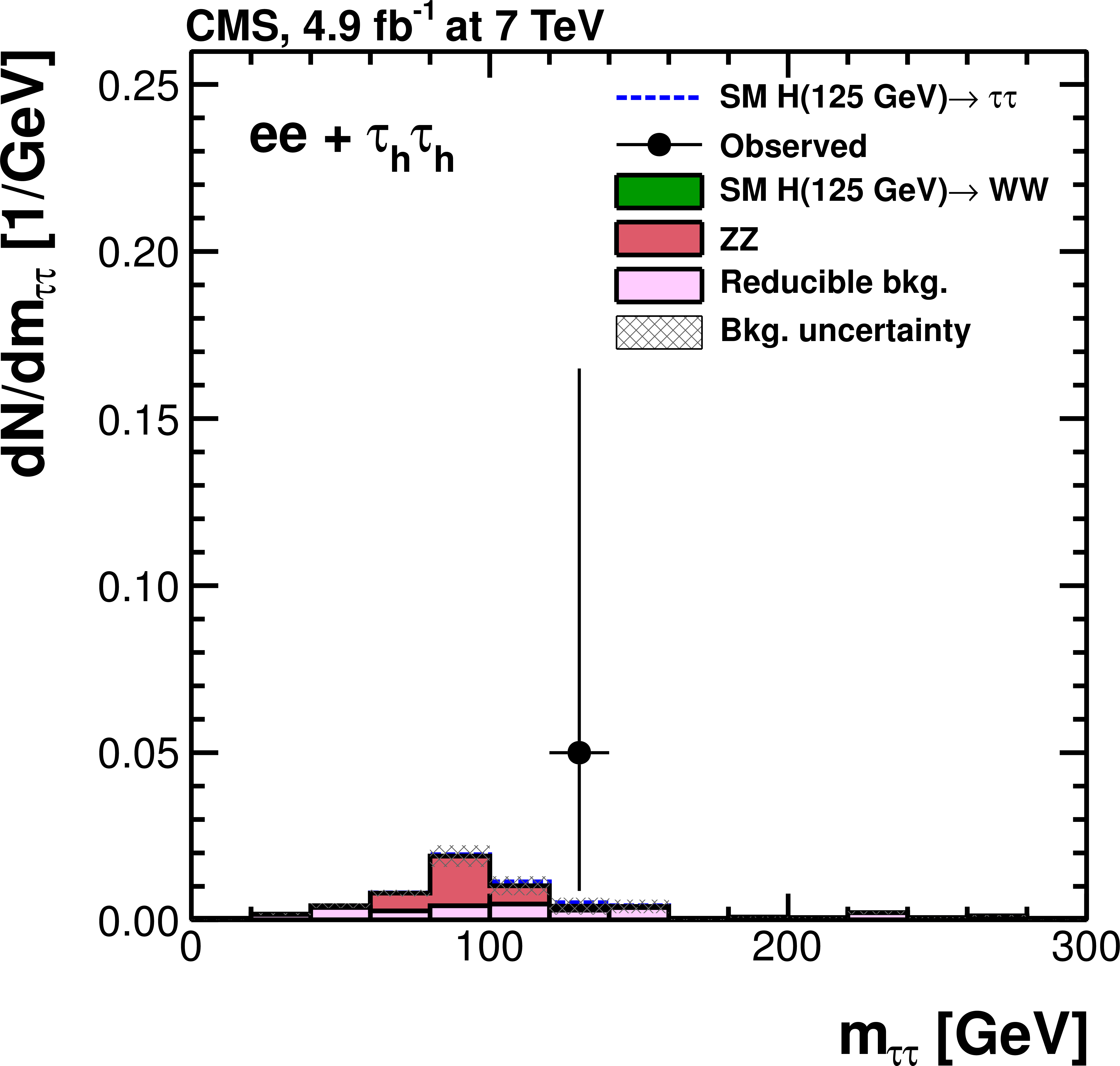
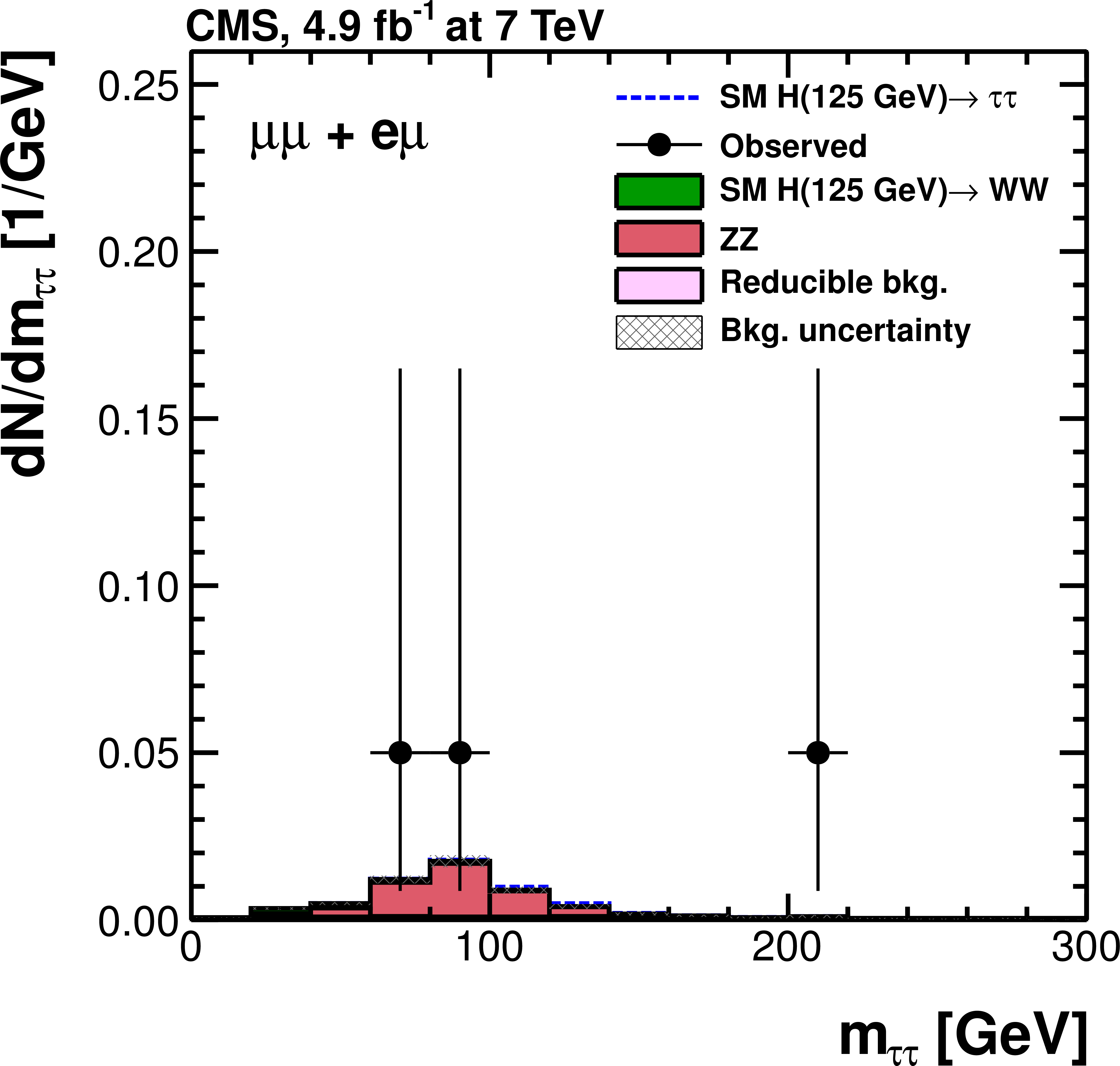
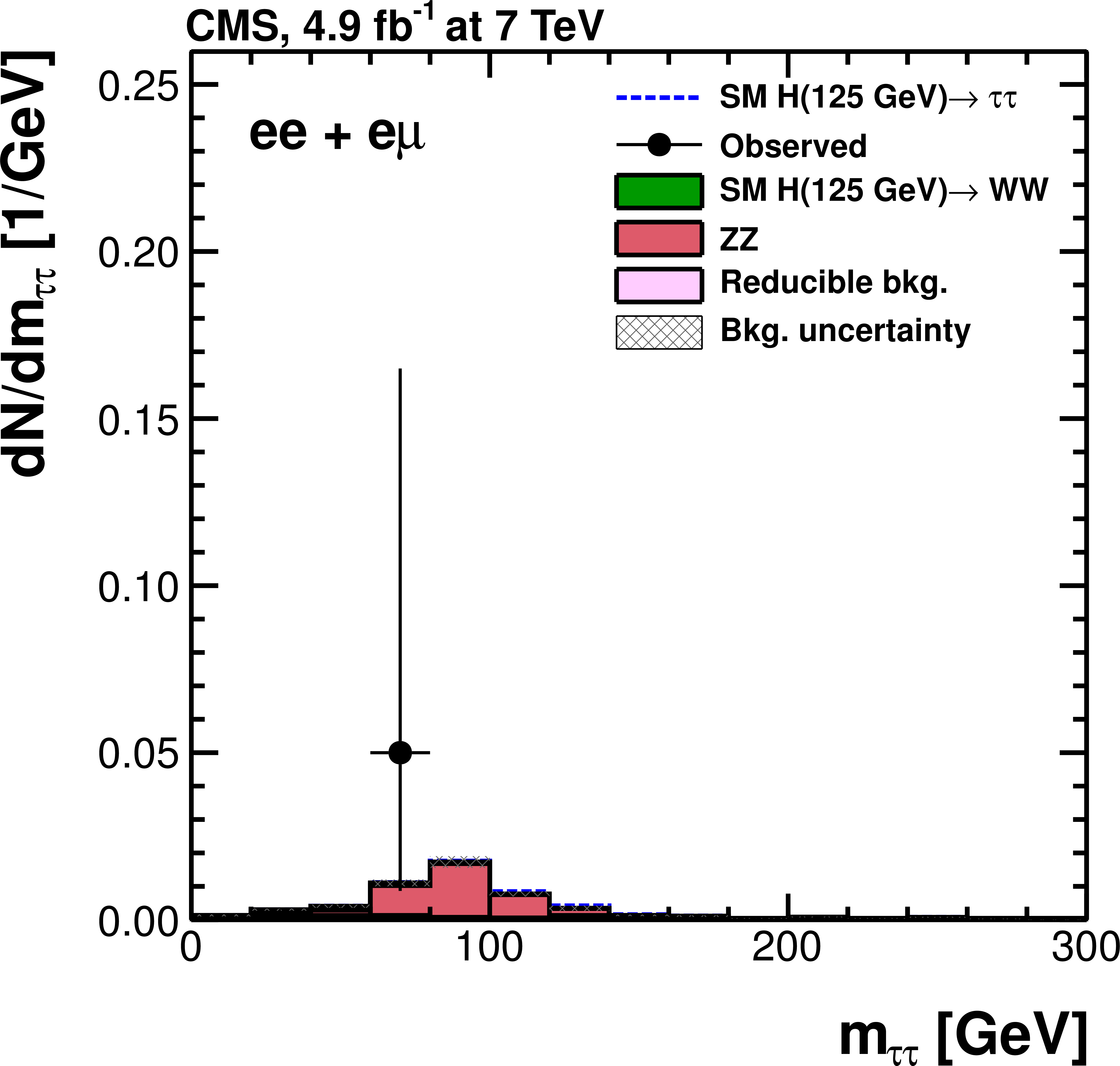
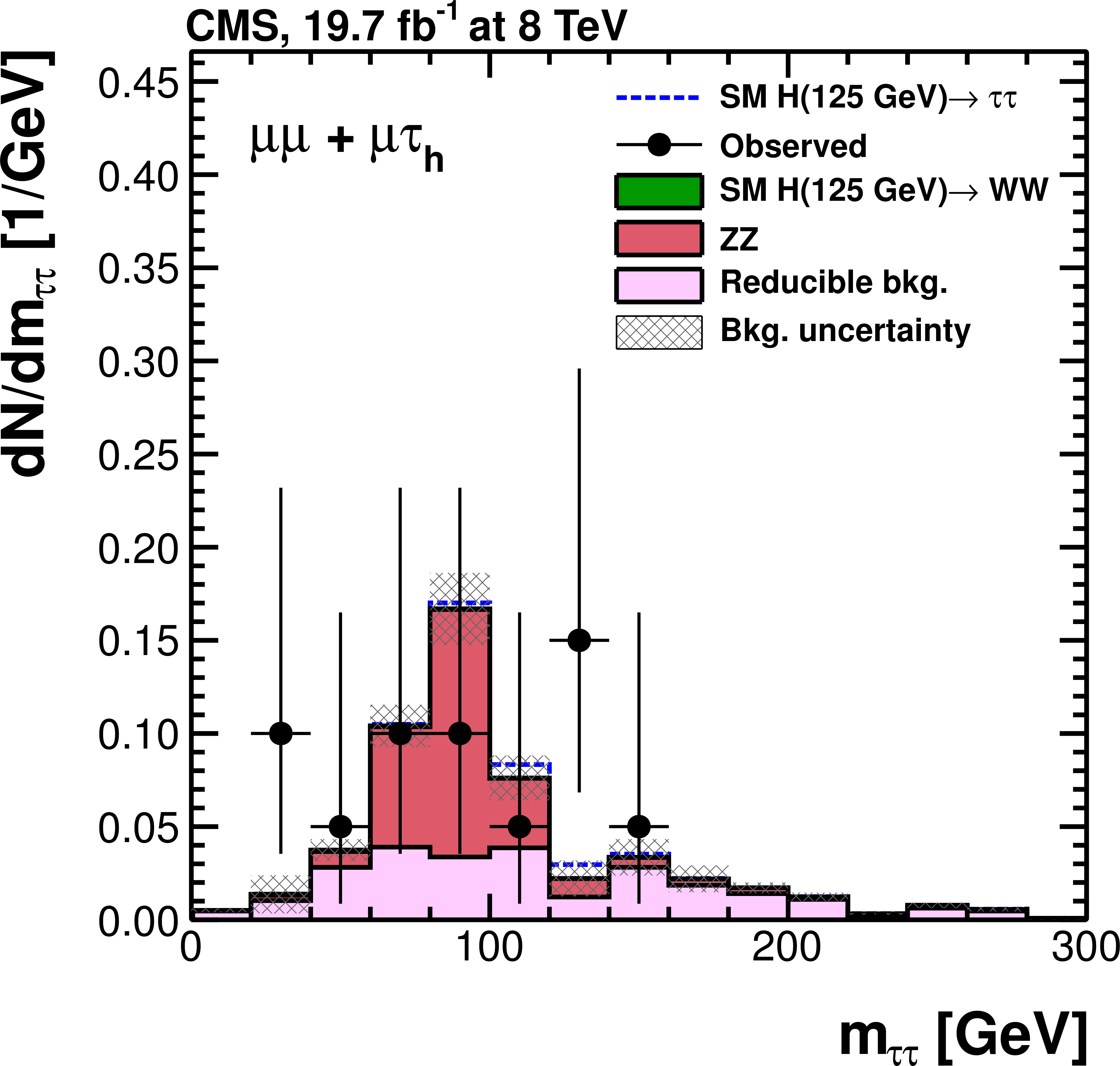
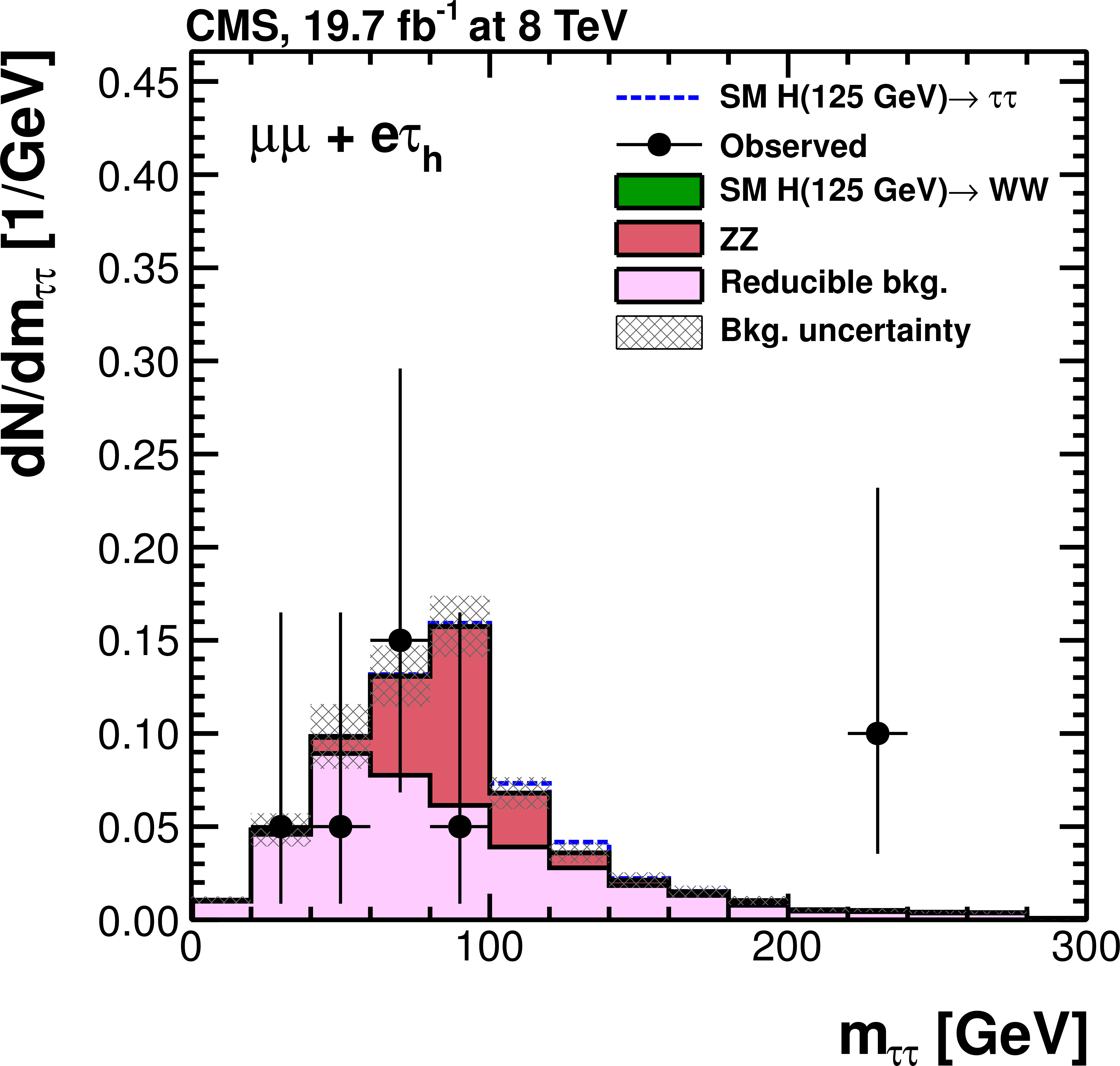
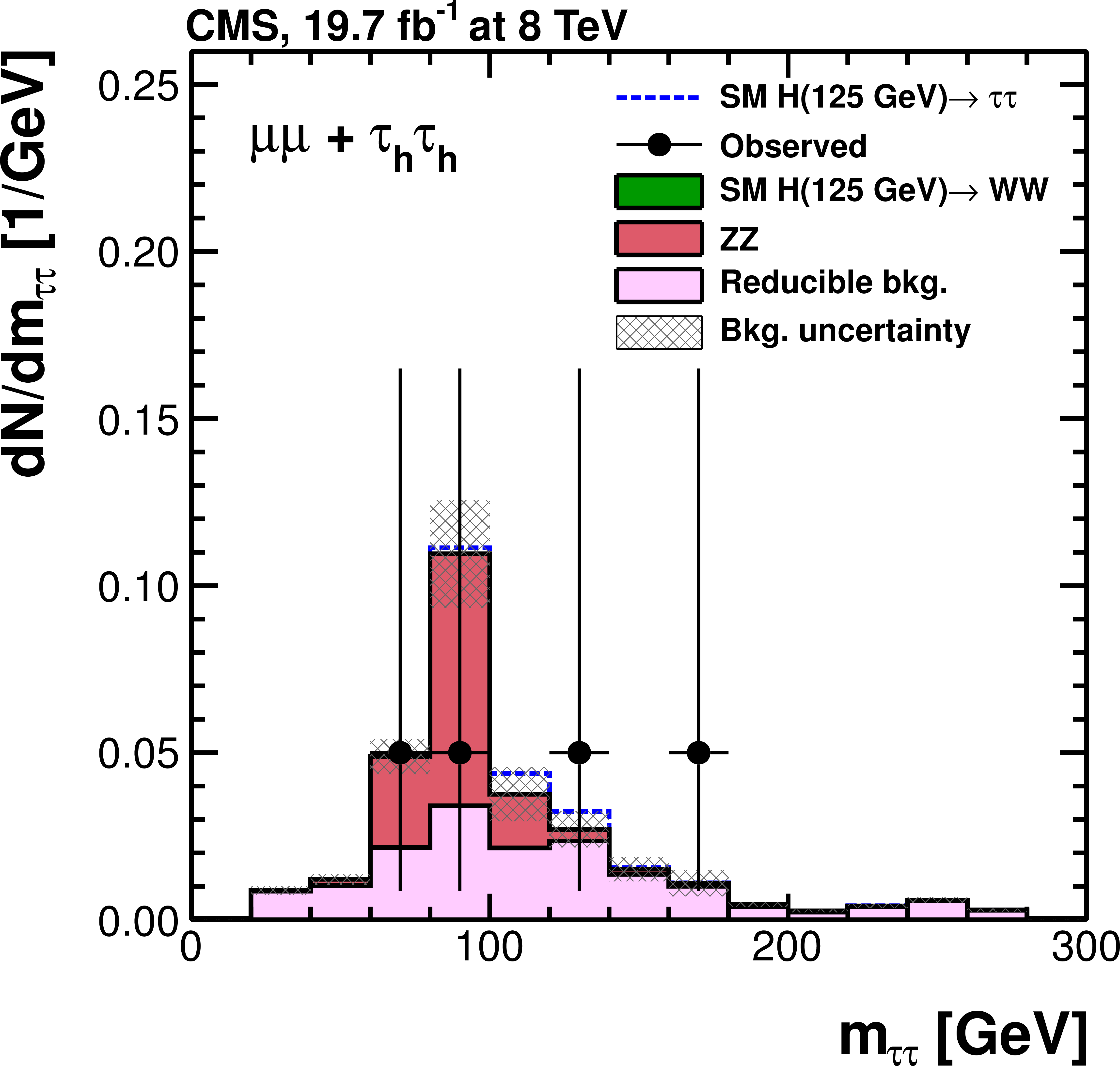
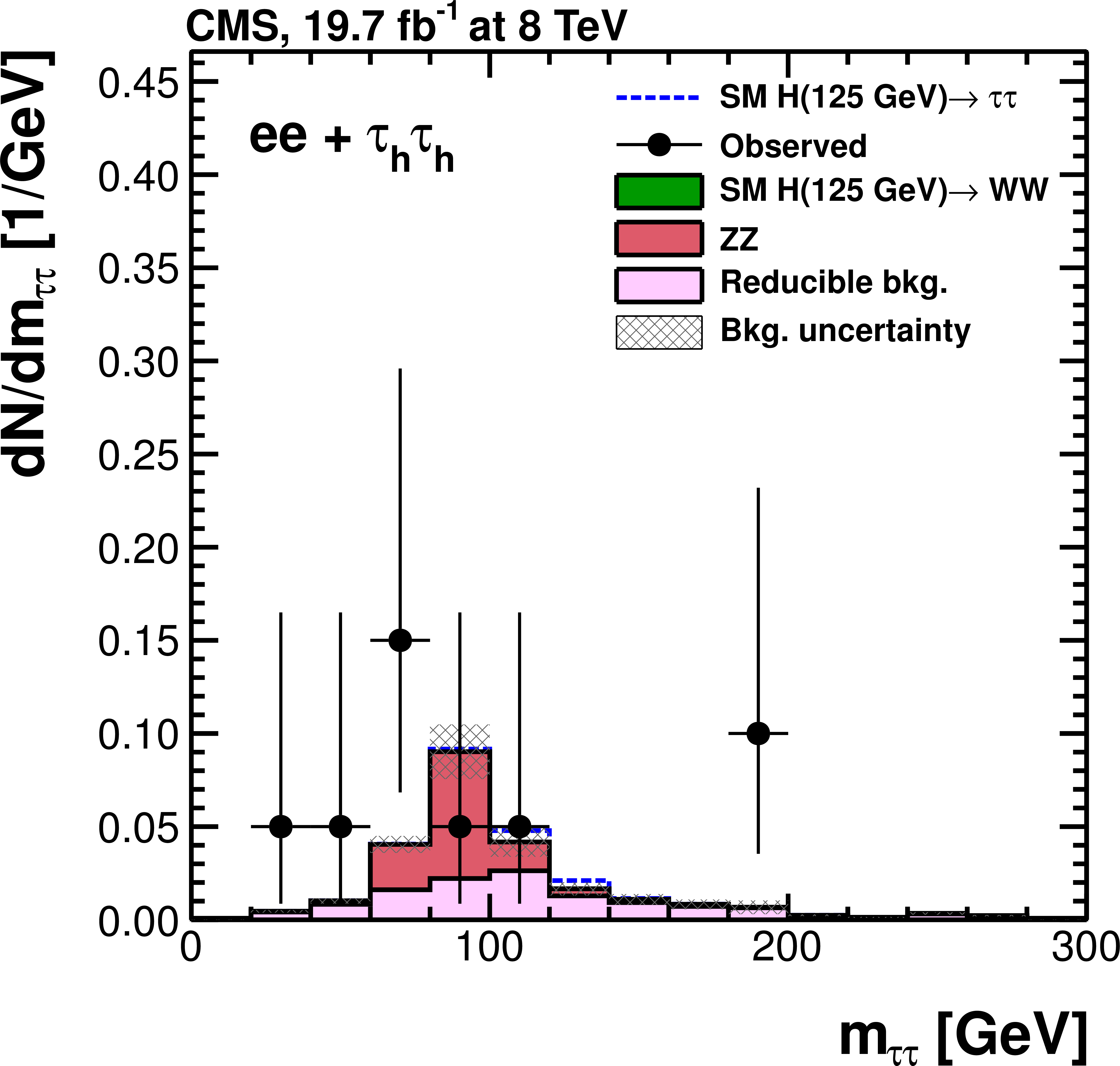
Figure 32-a:
Observed and predicted $ {m_{ {\tau } {\tau }}} $ distributions for the four different $LL'$ final states of the $ {\mathrm {e}} {\mathrm {e}}+ LL'$ (a) and $ {{\mu }} {{\mu }}+ LL'$ (b) channels for the 8 TeV data analysis. The normalization of the predicted background distributions corresponds to the result of the global fit. The signal distribution, on the other hand, is normalized to the SM prediction. The signal and background histograms are stacked. |

png pdf |
Figure 32-b:
Observed and predicted $ {m_{ {\tau } {\tau }}} $ distributions for the four different $LL'$ final states of the $ {\mathrm {e}} {\mathrm {e}}+ LL'$ (a) and $ {{\mu }} {{\mu }}+ LL'$ (b) channels for the 8 TeV data analysis. The normalization of the predicted background distributions corresponds to the result of the global fit. The signal distribution, on the other hand, is normalized to the SM prediction. The signal and background histograms are stacked. |
png pdf |
Figure 32-c:
Observed and predicted $ {m_{ {\tau } {\tau }}} $ distributions for the four different $LL'$ final states of the $ {\mathrm {e}} {\mathrm {e}}+ LL'$ (a) and $ {{\mu }} {{\mu }}+ LL'$ (b) channels for the 8 TeV data analysis. The normalization of the predicted background distributions corresponds to the result of the global fit. The signal distribution, on the other hand, is normalized to the SM prediction. The signal and background histograms are stacked. |

png pdf |
Figure 32-d:
Observed and predicted $ {m_{ {\tau } {\tau }}} $ distributions for the four different $LL'$ final states of the $ {\mathrm {e}} {\mathrm {e}}+ LL'$ (a) and $ {{\mu }} {{\mu }}+ LL'$ (b) channels for the 8 TeV data analysis. The normalization of the predicted background distributions corresponds to the result of the global fit. The signal distribution, on the other hand, is normalized to the SM prediction. The signal and background histograms are stacked. |
png pdf |
Figure 32-e:
Observed and predicted $ {m_{ {\tau } {\tau }}} $ distributions for the four different $LL'$ final states of the $ {\mathrm {e}} {\mathrm {e}}+ LL'$ (a) and $ {{\mu }} {{\mu }}+ LL'$ (b) channels for the 8 TeV data analysis. The normalization of the predicted background distributions corresponds to the result of the global fit. The signal distribution, on the other hand, is normalized to the SM prediction. The signal and background histograms are stacked. |
png pdf |
Figure 32-f:
Observed and predicted $ {m_{ {\tau } {\tau }}} $ distributions for the four different $LL'$ final states of the $ {\mathrm {e}} {\mathrm {e}}+ LL'$ (a) and $ {{\mu }} {{\mu }}+ LL'$ (b) channels for the 8 TeV data analysis. The normalization of the predicted background distributions corresponds to the result of the global fit. The signal distribution, on the other hand, is normalized to the SM prediction. The signal and background histograms are stacked. |
png pdf |
Figure 32-g:
Observed and predicted $ {m_{ {\tau } {\tau }}} $ distributions for the four different $LL'$ final states of the $ {\mathrm {e}} {\mathrm {e}}+ LL'$ (a) and $ {{\mu }} {{\mu }}+ LL'$ (b) channels for the 8 TeV data analysis. The normalization of the predicted background distributions corresponds to the result of the global fit. The signal distribution, on the other hand, is normalized to the SM prediction. The signal and background histograms are stacked. |

png pdf |
Figure 32-h:
Observed and predicted $ {m_{ {\tau } {\tau }}} $ distributions for the four different $LL'$ final states of the $ {\mathrm {e}} {\mathrm {e}}+ LL'$ (a) and $ {{\mu }} {{\mu }}+ LL'$ (b) channels for the 8 TeV data analysis. The normalization of the predicted background distributions corresponds to the result of the global fit. The signal distribution, on the other hand, is normalized to the SM prediction. The signal and background histograms are stacked. |
|
|
Compact Muon Solenoid LHC, CERN |
|

|

|

|

|

|