

Compact Muon Solenoid
LHC, CERN
| CMS-HIG-14-005 ; CERN-PH-EP-2015-027 | ||
| Search for lepton-flavour-violating decays of the Higgs boson | ||
| CMS Collaboration | ||
| 26 February 2015 | ||
| Phys. Lett. B 749 (2015) 337 | ||
| Abstract: The first direct search for lepton-flavour-violating decays of the recently discovered Higgs boson (H) is described. The search is performed in the $\mathrm{H \to \mu \tau_e}$ and $\mathrm{H \to \mu \tau_h}$ channels, where $\mathrm{\tau_e}$ and $\mathrm{\tau_h}$ are tau leptons reconstructed in the electronic and hadronic decay channels, respectively. The data sample used in this search was collected in pp collisions at a centre-of-mass energy of $\sqrt{s}$ = 8 TeV with the CMS experiment at the CERN LHC and corresponds to an integrated luminosity of 19.7 fb$^{-1}$. The sensitivity of the search is an order of magnitude better than the existing indirect limits. A slight excess of signal events with a significance of 2.4 standard deviations is observed. The $p$-value of this excess at $M_{\mathrm{H}} = $ 125 GeV is 0.010. The best fit branching fraction is $\mathcal{B}(\mathrm{H \to \mu \tau} )= $ (0.84 $^{+0.39}_{-0.37}$)%. A constraint on the branching fraction, $\mathcal{B}(\mathrm{H \to \mu \tau})$ less than 1.51% at 95% confidence level, is set. This limit is subsequently used to constrain the $\mu$-$\tau$ Yukawa couplings to be less than 3.6 $\times$ 10$^{-3}$. | ||
| Links: e-print arXiv:1502.07400 [hep-ex] (PDF) ; CDS record ; inSPIRE record ; Public twiki page ; CADI line (restricted) ; | ||
| Figures | |
png pdf |
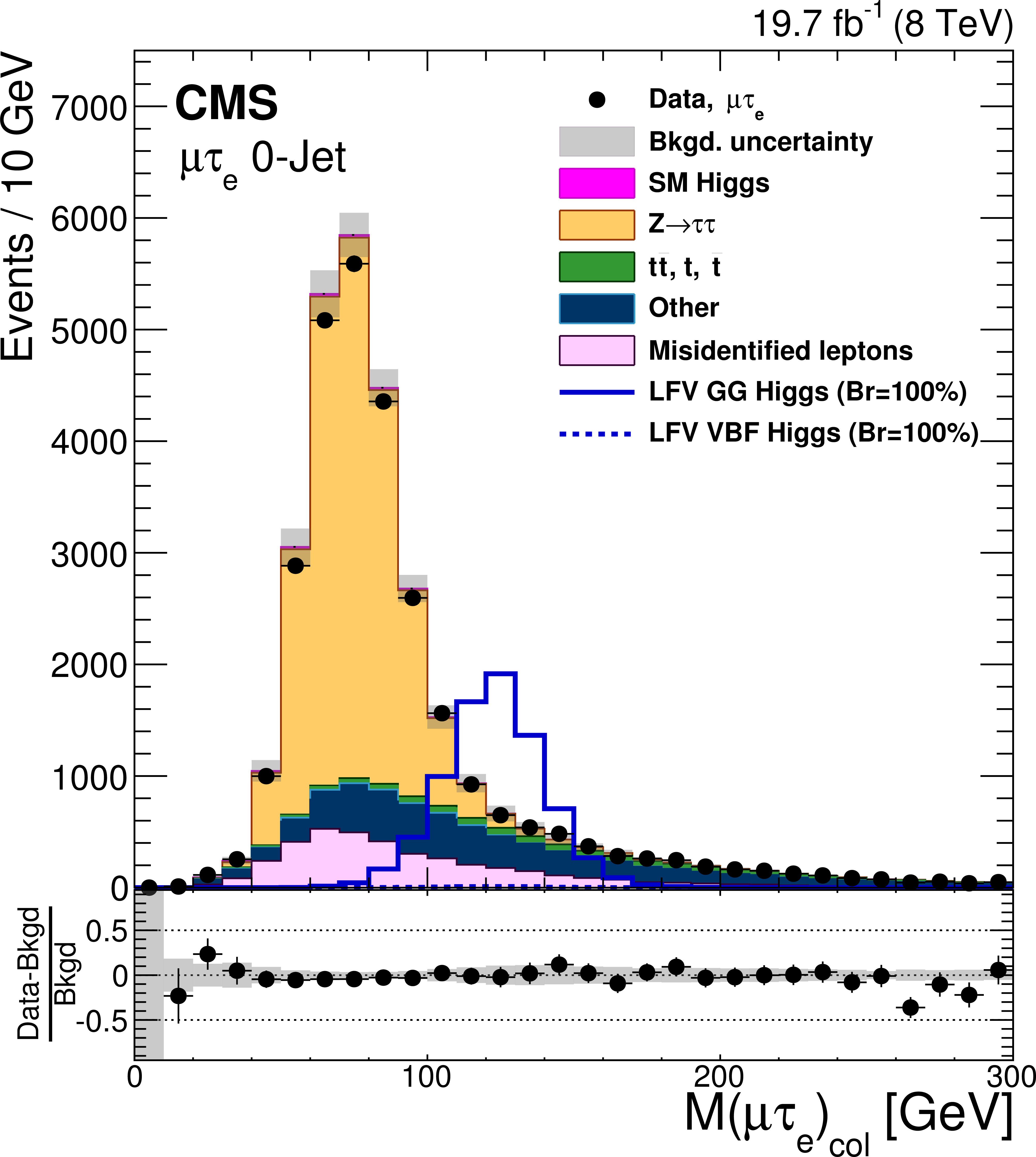
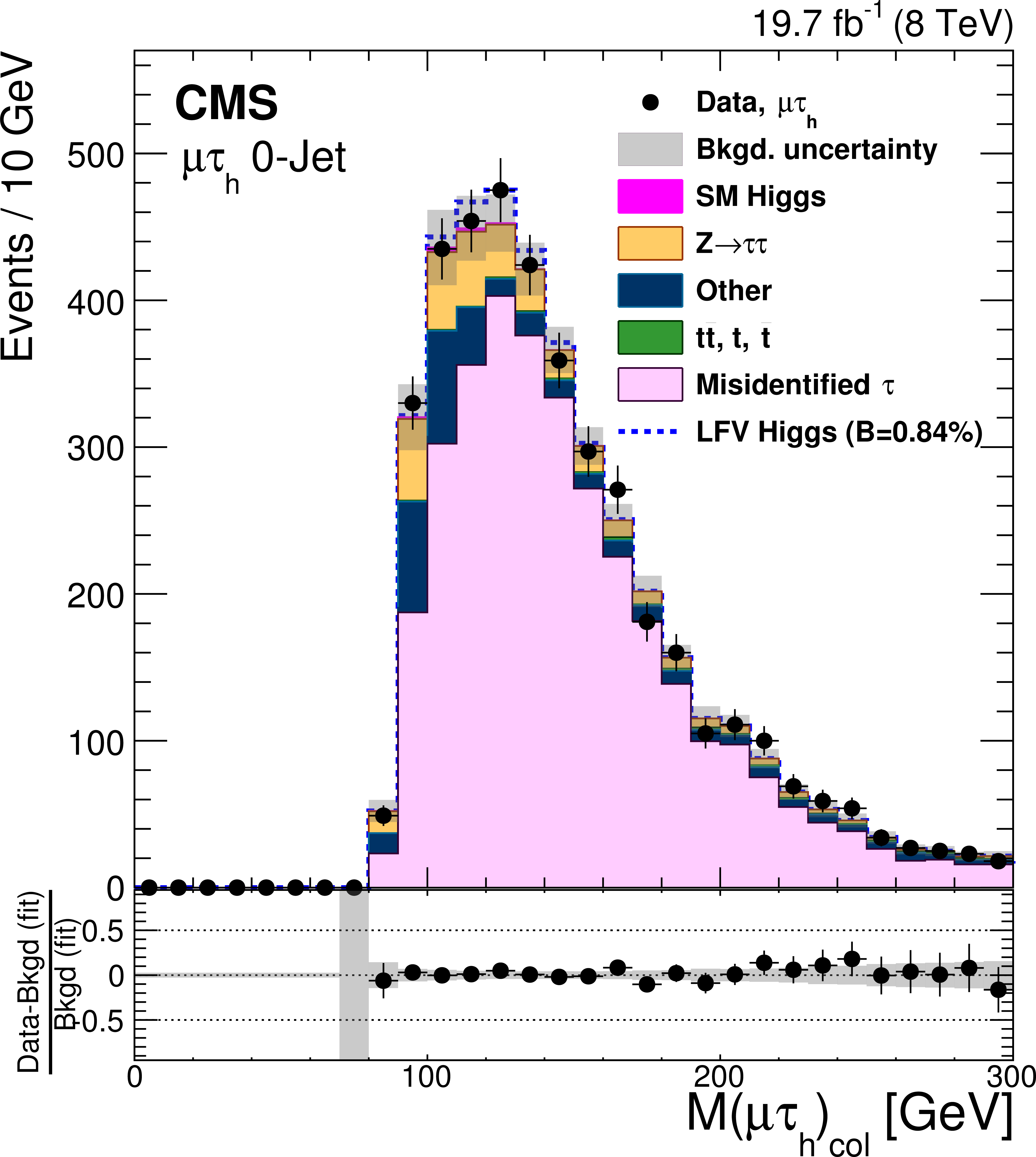
Figure 1-a:
Distributions of the collinear mass $M_\text {col}$ for signal ($\mathcal {B}( {\mathrm {H}} \to {{\mu }} {\tau })=$ 100% for clarity) and background after the loose selection requirements for the LFV $ {\mathrm {H}} \to {{\mu }} {\tau }$ candidates for the different channels and categories compared to data. The shaded grey bands indicate the total uncertainty. The bottom panel in each plot shows the fractional difference between the observed data and the total estimated background. a: $ {\mathrm {H}} \to {{\mu }} {\tau }_{ {\mathrm {e}}}$ 0-jet; b: $ {\mathrm {H}} \to {{\mu }} { {\tau }_\mathrm {h}} $ 0-jet; c: $ {\mathrm {H}} \to {{\mu }} {\tau }_{ {\mathrm {e}}}$ 1-jet; d: $ {\mathrm {H}} \to {{\mu }} { {\tau }_\mathrm {h}} $ 1-jet; e: $ {\mathrm {H}} \to {{\mu }} {\tau }_{ {\mathrm {e}}}$ 2-jet; f $ {\mathrm {H}} \to {{\mu }} { {\tau }_\mathrm {h}} $ 2-jet. |
png pdf |
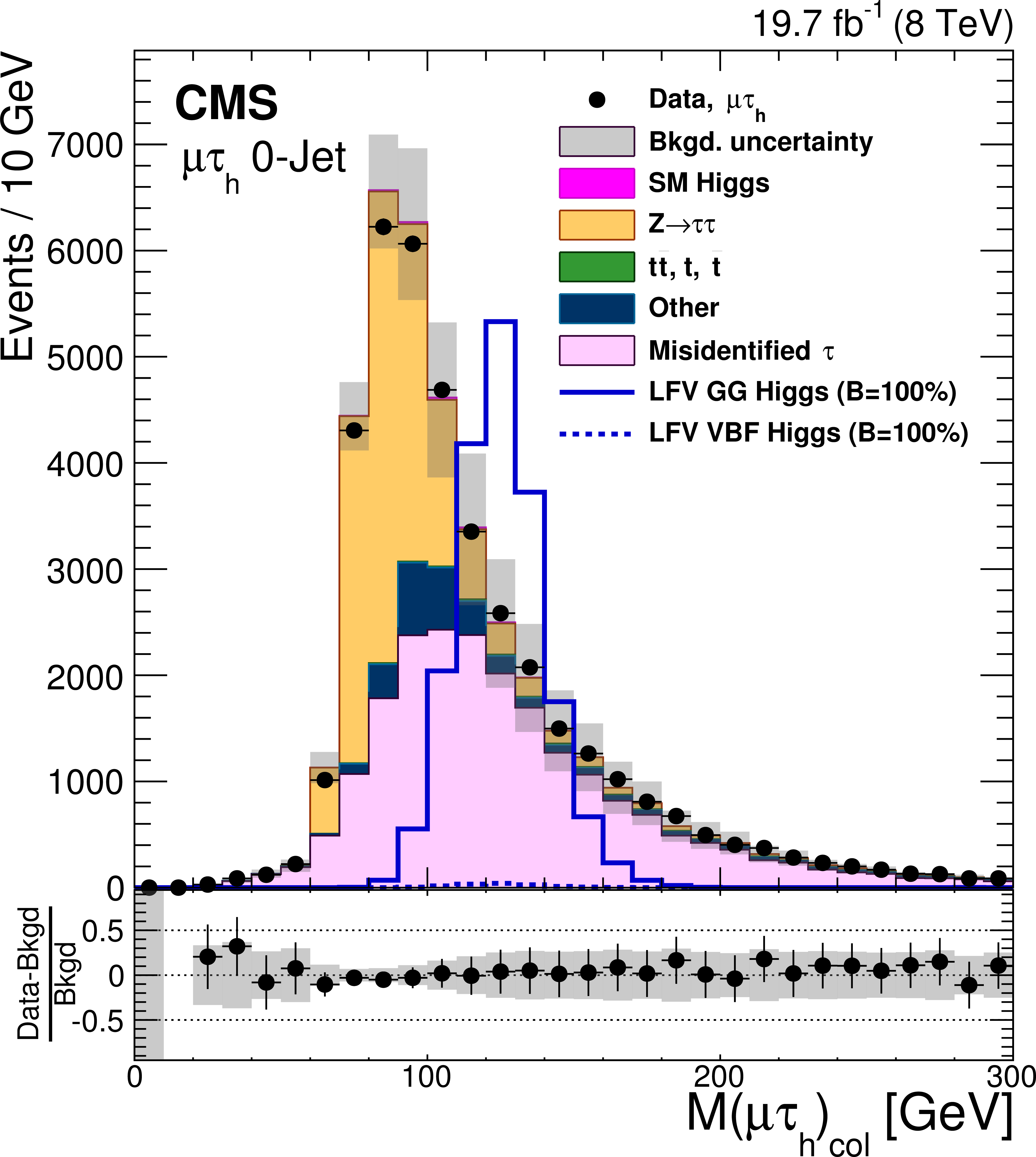
Figure 1-b:
Distributions of the collinear mass $M_\text {col}$ for signal ($\mathcal {B}( {\mathrm {H}} \to {{\mu }} {\tau })=$ 100% for clarity) and background after the loose selection requirements for the LFV $ {\mathrm {H}} \to {{\mu }} {\tau }$ candidates for the different channels and categories compared to data. The shaded grey bands indicate the total uncertainty. The bottom panel in each plot shows the fractional difference between the observed data and the total estimated background. a: $ {\mathrm {H}} \to {{\mu }} {\tau }_{ {\mathrm {e}}}$ 0-jet; b: $ {\mathrm {H}} \to {{\mu }} { {\tau }_\mathrm {h}} $ 0-jet; c: $ {\mathrm {H}} \to {{\mu }} {\tau }_{ {\mathrm {e}}}$ 1-jet; d: $ {\mathrm {H}} \to {{\mu }} { {\tau }_\mathrm {h}} $ 1-jet; e: $ {\mathrm {H}} \to {{\mu }} {\tau }_{ {\mathrm {e}}}$ 2-jet; f $ {\mathrm {H}} \to {{\mu }} { {\tau }_\mathrm {h}} $ 2-jet. |
png pdf |
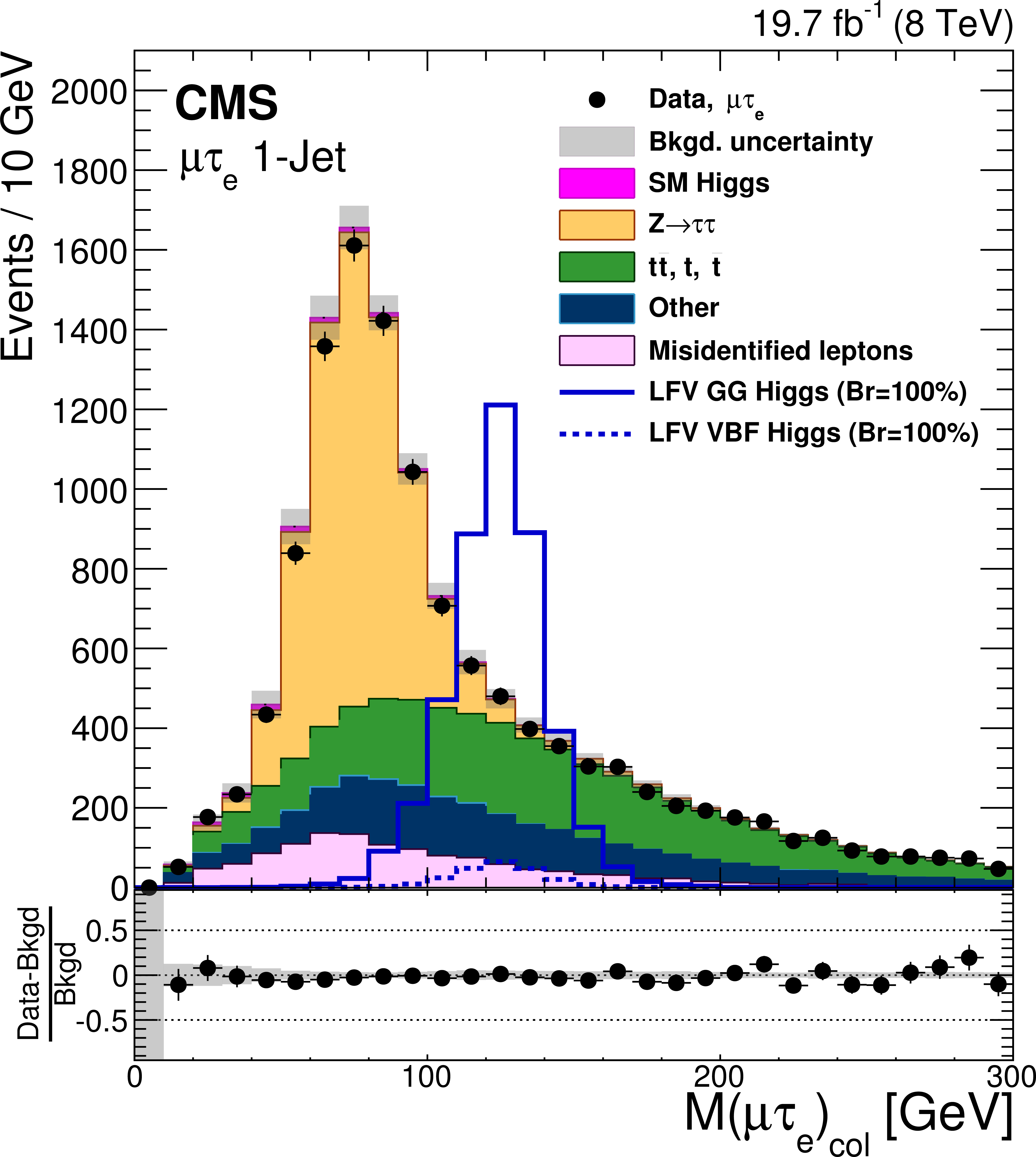
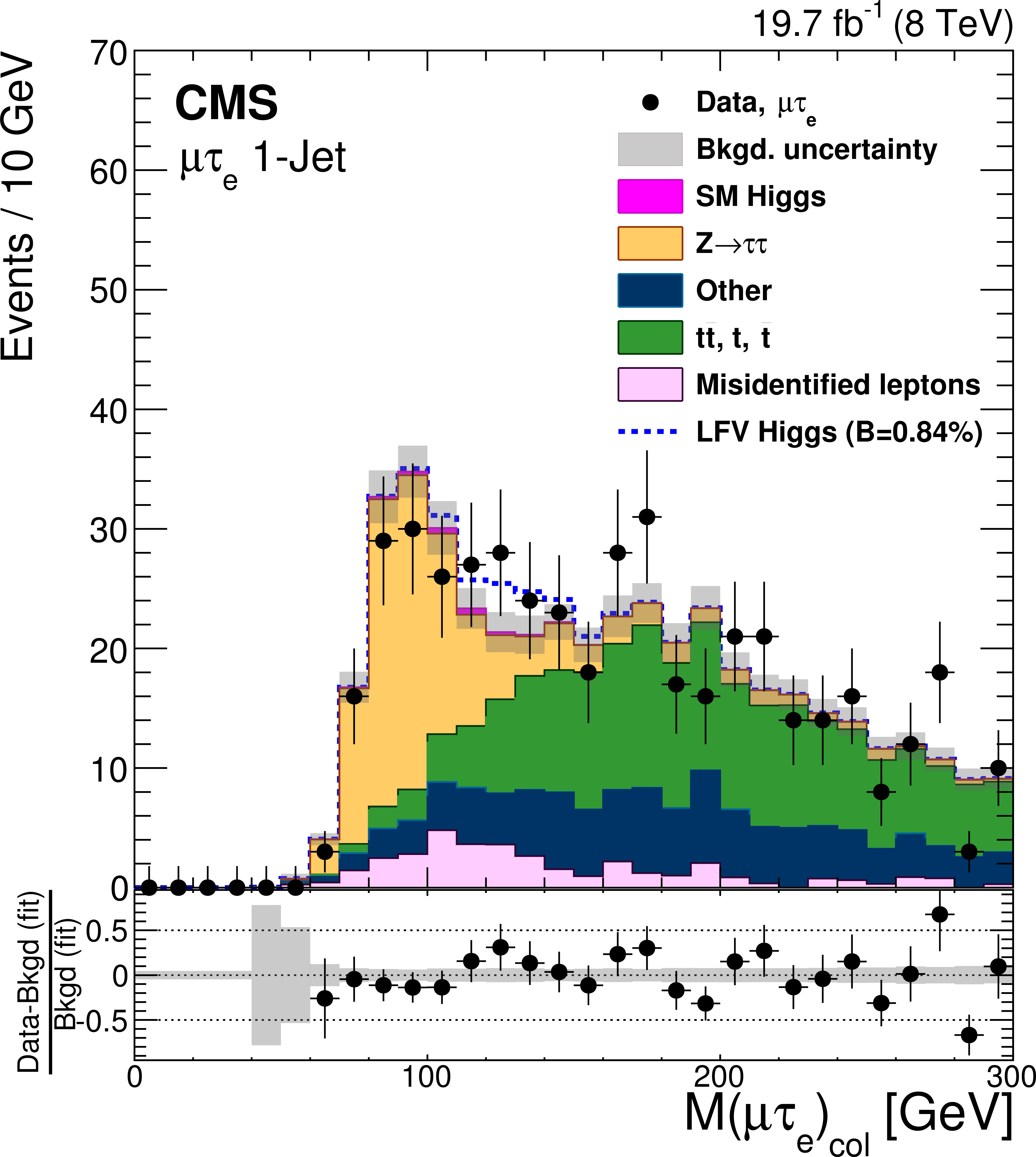
Figure 1-c:
Distributions of the collinear mass $M_\text {col}$ for signal ($\mathcal {B}( {\mathrm {H}} \to {{\mu }} {\tau })=$ 100% for clarity) and background after the loose selection requirements for the LFV $ {\mathrm {H}} \to {{\mu }} {\tau }$ candidates for the different channels and categories compared to data. The shaded grey bands indicate the total uncertainty. The bottom panel in each plot shows the fractional difference between the observed data and the total estimated background. a: $ {\mathrm {H}} \to {{\mu }} {\tau }_{ {\mathrm {e}}}$ 0-jet; b: $ {\mathrm {H}} \to {{\mu }} { {\tau }_\mathrm {h}} $ 0-jet; c: $ {\mathrm {H}} \to {{\mu }} {\tau }_{ {\mathrm {e}}}$ 1-jet; d: $ {\mathrm {H}} \to {{\mu }} { {\tau }_\mathrm {h}} $ 1-jet; e: $ {\mathrm {H}} \to {{\mu }} {\tau }_{ {\mathrm {e}}}$ 2-jet; f $ {\mathrm {H}} \to {{\mu }} { {\tau }_\mathrm {h}} $ 2-jet. |
png pdf |
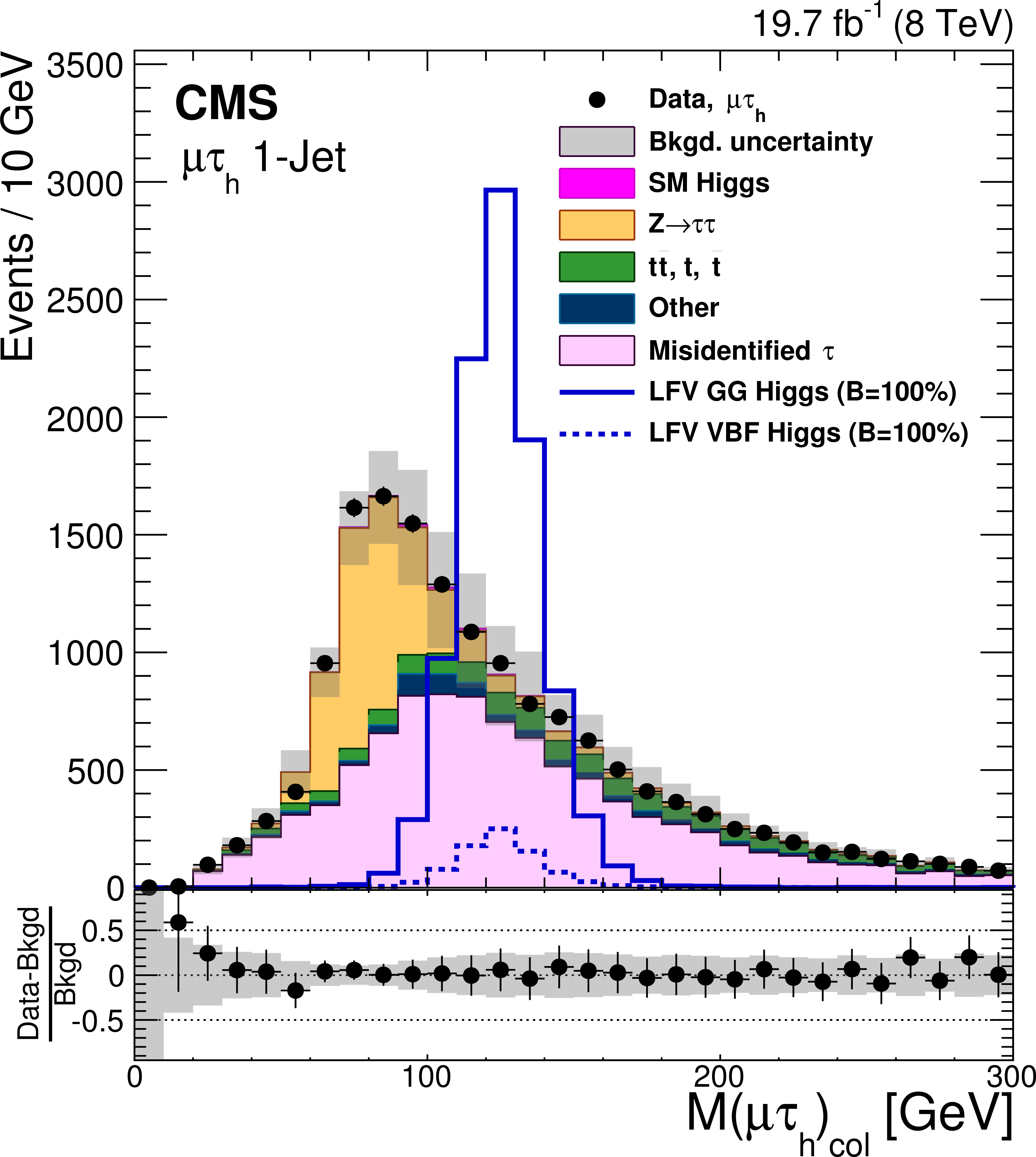
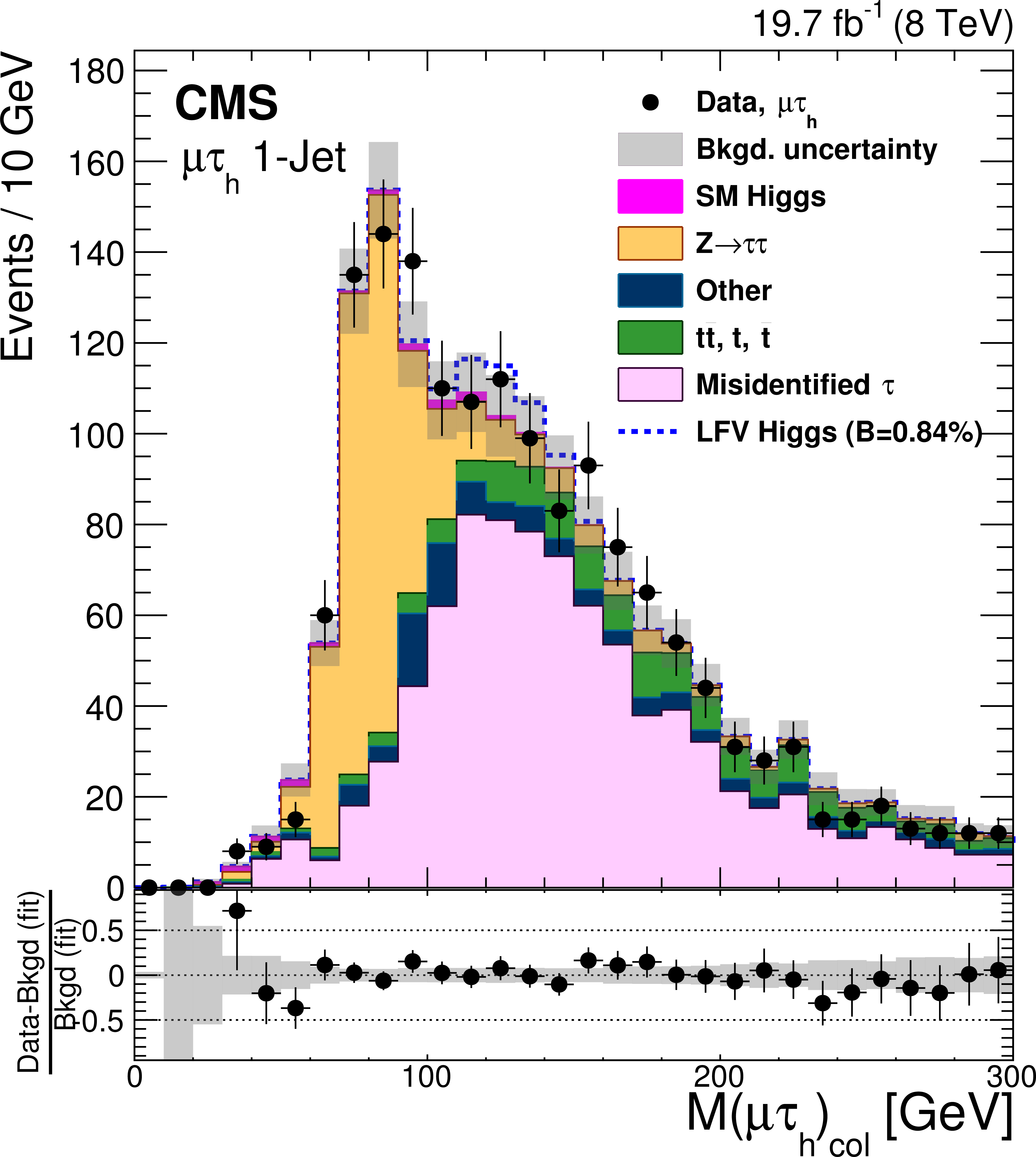
Figure 1-d:
Distributions of the collinear mass $M_\text {col}$ for signal ($\mathcal {B}( {\mathrm {H}} \to {{\mu }} {\tau })=$ 100% for clarity) and background after the loose selection requirements for the LFV $ {\mathrm {H}} \to {{\mu }} {\tau }$ candidates for the different channels and categories compared to data. The shaded grey bands indicate the total uncertainty. The bottom panel in each plot shows the fractional difference between the observed data and the total estimated background. a: $ {\mathrm {H}} \to {{\mu }} {\tau }_{ {\mathrm {e}}}$ 0-jet; b: $ {\mathrm {H}} \to {{\mu }} { {\tau }_\mathrm {h}} $ 0-jet; c: $ {\mathrm {H}} \to {{\mu }} {\tau }_{ {\mathrm {e}}}$ 1-jet; d: $ {\mathrm {H}} \to {{\mu }} { {\tau }_\mathrm {h}} $ 1-jet; e: $ {\mathrm {H}} \to {{\mu }} {\tau }_{ {\mathrm {e}}}$ 2-jet; f $ {\mathrm {H}} \to {{\mu }} { {\tau }_\mathrm {h}} $ 2-jet. |
png pdf |
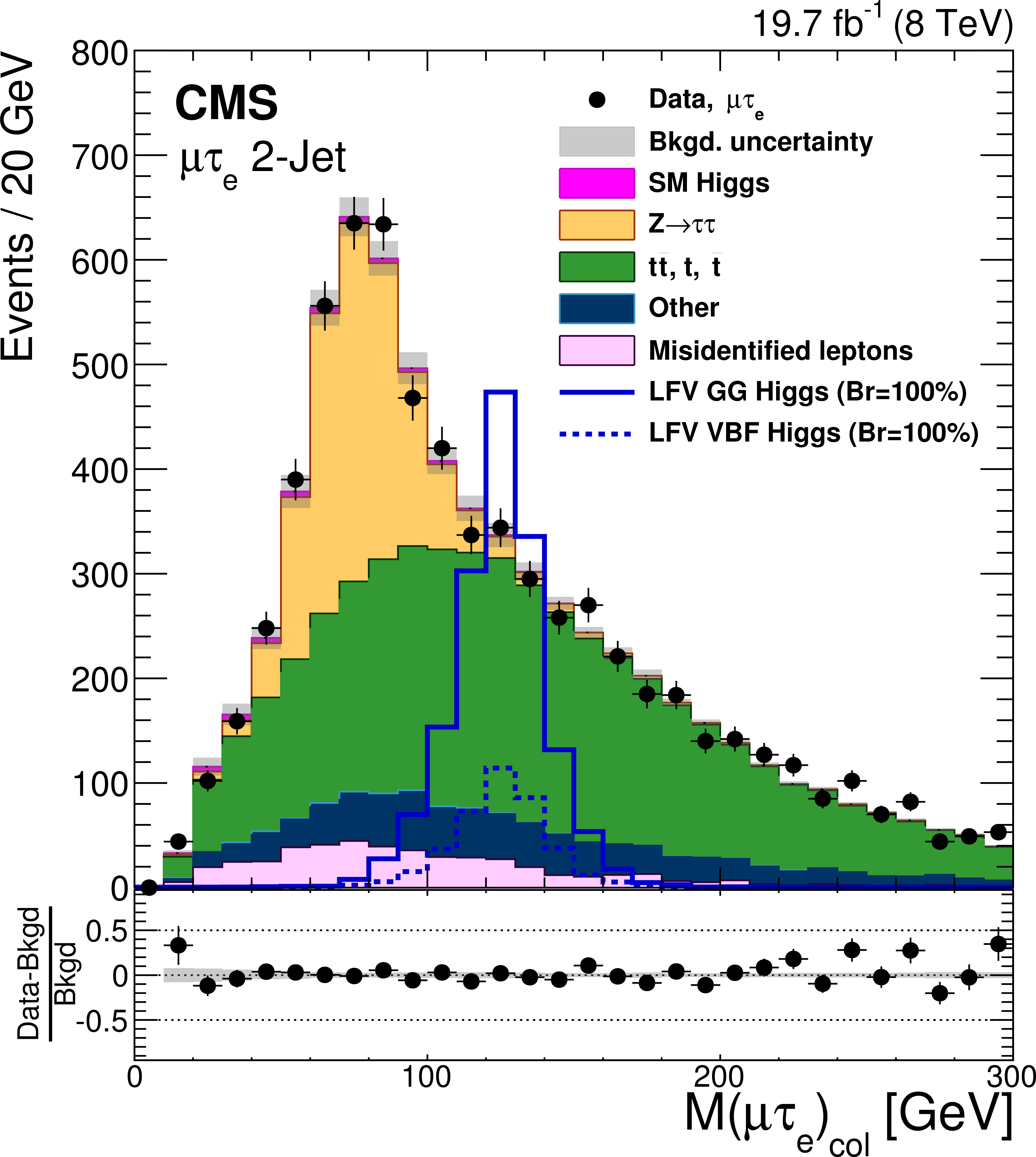
Figure 1-e:
Distributions of the collinear mass $M_\text {col}$ for signal ($\mathcal {B}( {\mathrm {H}} \to {{\mu }} {\tau })=$ 100% for clarity) and background after the loose selection requirements for the LFV $ {\mathrm {H}} \to {{\mu }} {\tau }$ candidates for the different channels and categories compared to data. The shaded grey bands indicate the total uncertainty. The bottom panel in each plot shows the fractional difference between the observed data and the total estimated background. a: $ {\mathrm {H}} \to {{\mu }} {\tau }_{ {\mathrm {e}}}$ 0-jet; b: $ {\mathrm {H}} \to {{\mu }} { {\tau }_\mathrm {h}} $ 0-jet; c: $ {\mathrm {H}} \to {{\mu }} {\tau }_{ {\mathrm {e}}}$ 1-jet; d: $ {\mathrm {H}} \to {{\mu }} { {\tau }_\mathrm {h}} $ 1-jet; e: $ {\mathrm {H}} \to {{\mu }} {\tau }_{ {\mathrm {e}}}$ 2-jet; f $ {\mathrm {H}} \to {{\mu }} { {\tau }_\mathrm {h}} $ 2-jet. |
png pdf |
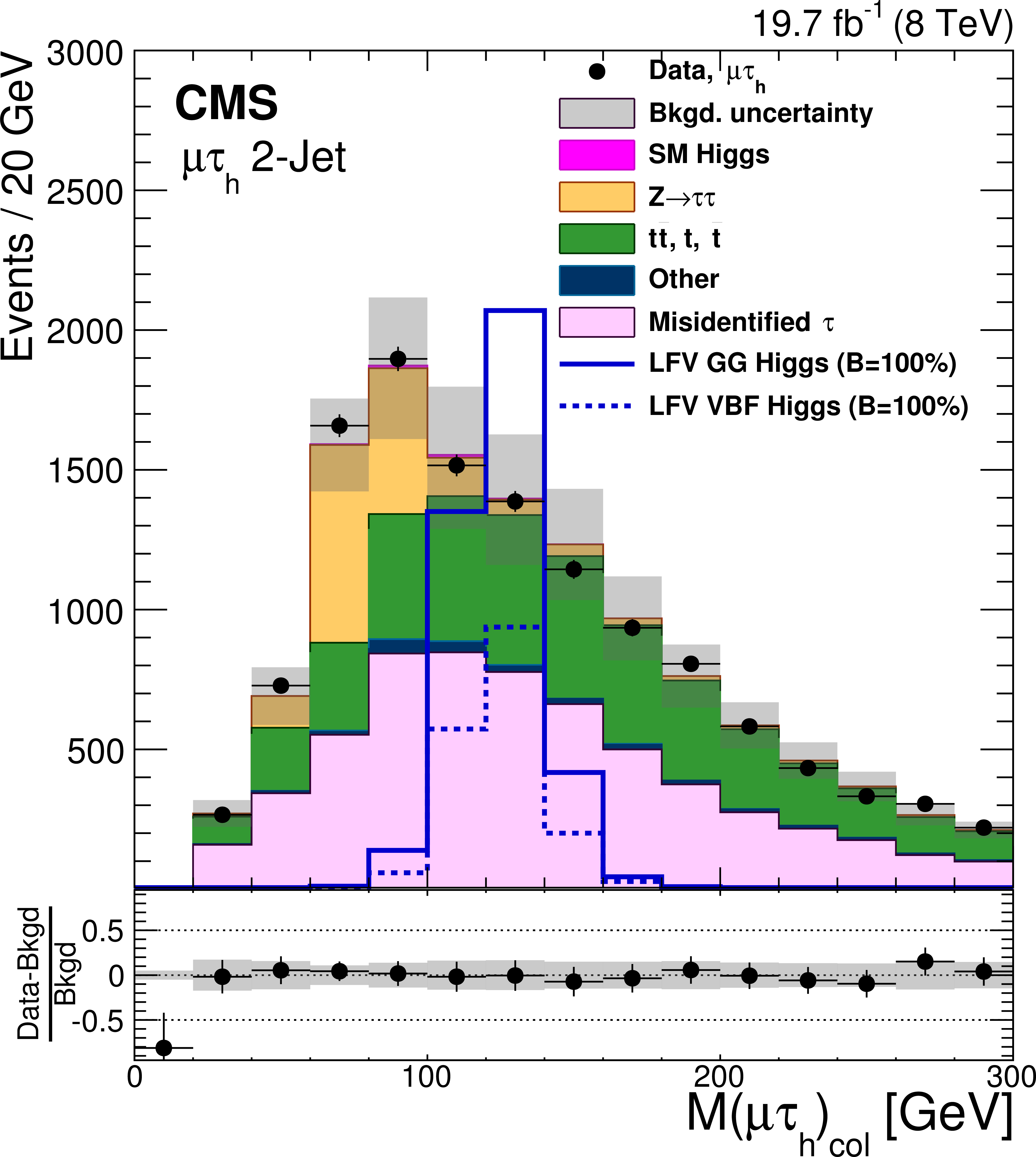
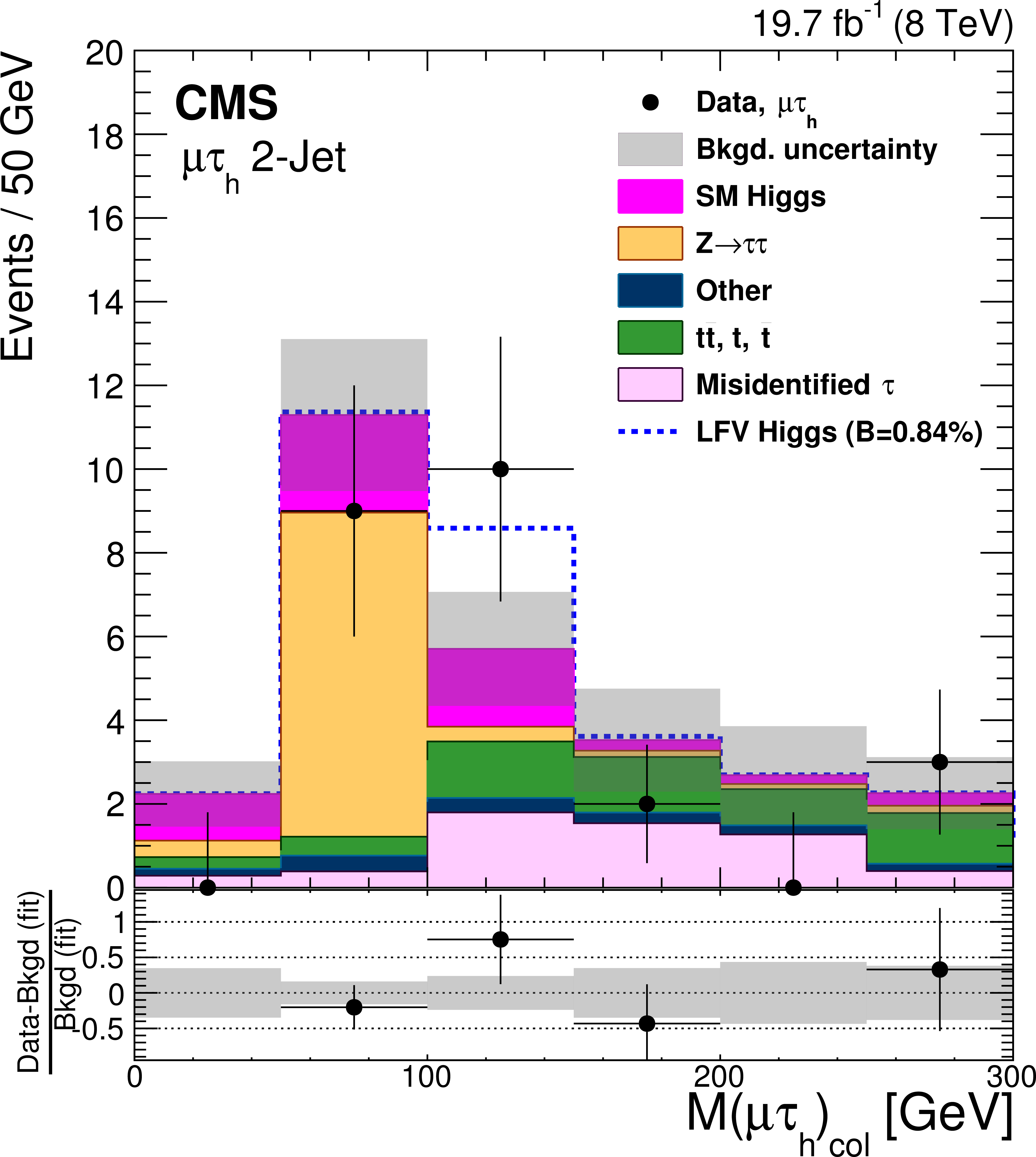
Figure 1-f:
Distributions of the collinear mass $M_\text {col}$ for signal ($\mathcal {B}( {\mathrm {H}} \to {{\mu }} {\tau })=$ 100% for clarity) and background after the loose selection requirements for the LFV $ {\mathrm {H}} \to {{\mu }} {\tau }$ candidates for the different channels and categories compared to data. The shaded grey bands indicate the total uncertainty. The bottom panel in each plot shows the fractional difference between the observed data and the total estimated background. a: $ {\mathrm {H}} \to {{\mu }} {\tau }_{ {\mathrm {e}}}$ 0-jet; b: $ {\mathrm {H}} \to {{\mu }} { {\tau }_\mathrm {h}} $ 0-jet; c: $ {\mathrm {H}} \to {{\mu }} {\tau }_{ {\mathrm {e}}}$ 1-jet; d: $ {\mathrm {H}} \to {{\mu }} { {\tau }_\mathrm {h}} $ 1-jet; e: $ {\mathrm {H}} \to {{\mu }} {\tau }_{ {\mathrm {e}}}$ 2-jet; f $ {\mathrm {H}} \to {{\mu }} { {\tau }_\mathrm {h}} $ 2-jet. |
png pdf |
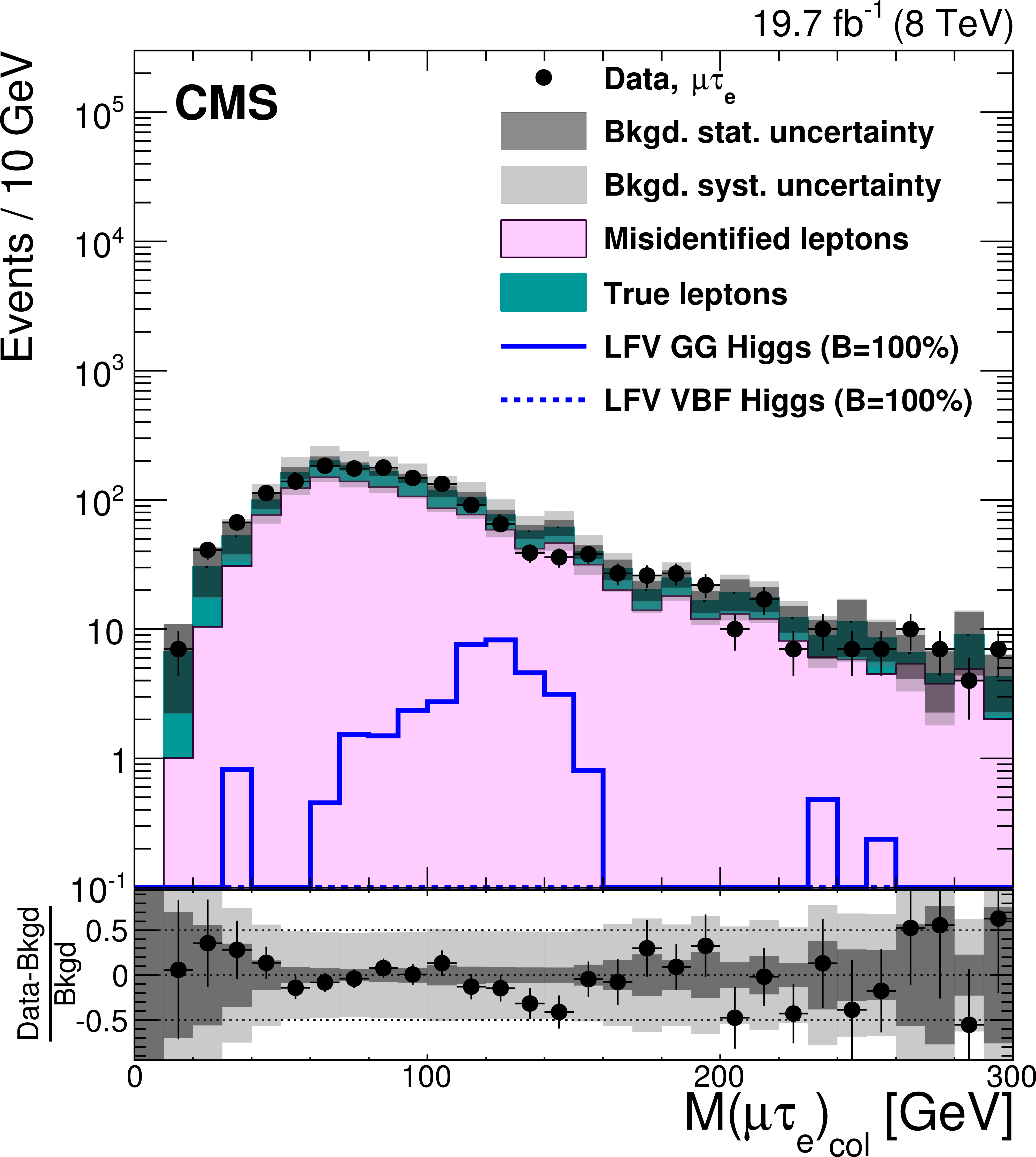
Figure 2-a:
Distributions of $M_\text {col}$ for region II compared to the estimate from scaling the region IV sample by the measured misidentification rates. The bottom panel in each plot shows the fractional difference between the observed data and the estimate. a: $ {\mathrm {H}} \to {{\mu }} {\tau }_{ {\mathrm {e}}}$. b: $ {\mathrm {H}} \to {{\mu }} { {\tau }_\mathrm {h}} $. |

png pdf |
Figure 2-b:
Distributions of $M_\text {col}$ for region II compared to the estimate from scaling the region IV sample by the measured misidentification rates. The bottom panel in each plot shows the fractional difference between the observed data and the estimate. a: $ {\mathrm {H}} \to {{\mu }} {\tau }_{ {\mathrm {e}}}$. b: $ {\mathrm {H}} \to {{\mu }} { {\tau }_\mathrm {h}} $. |
png pdf |
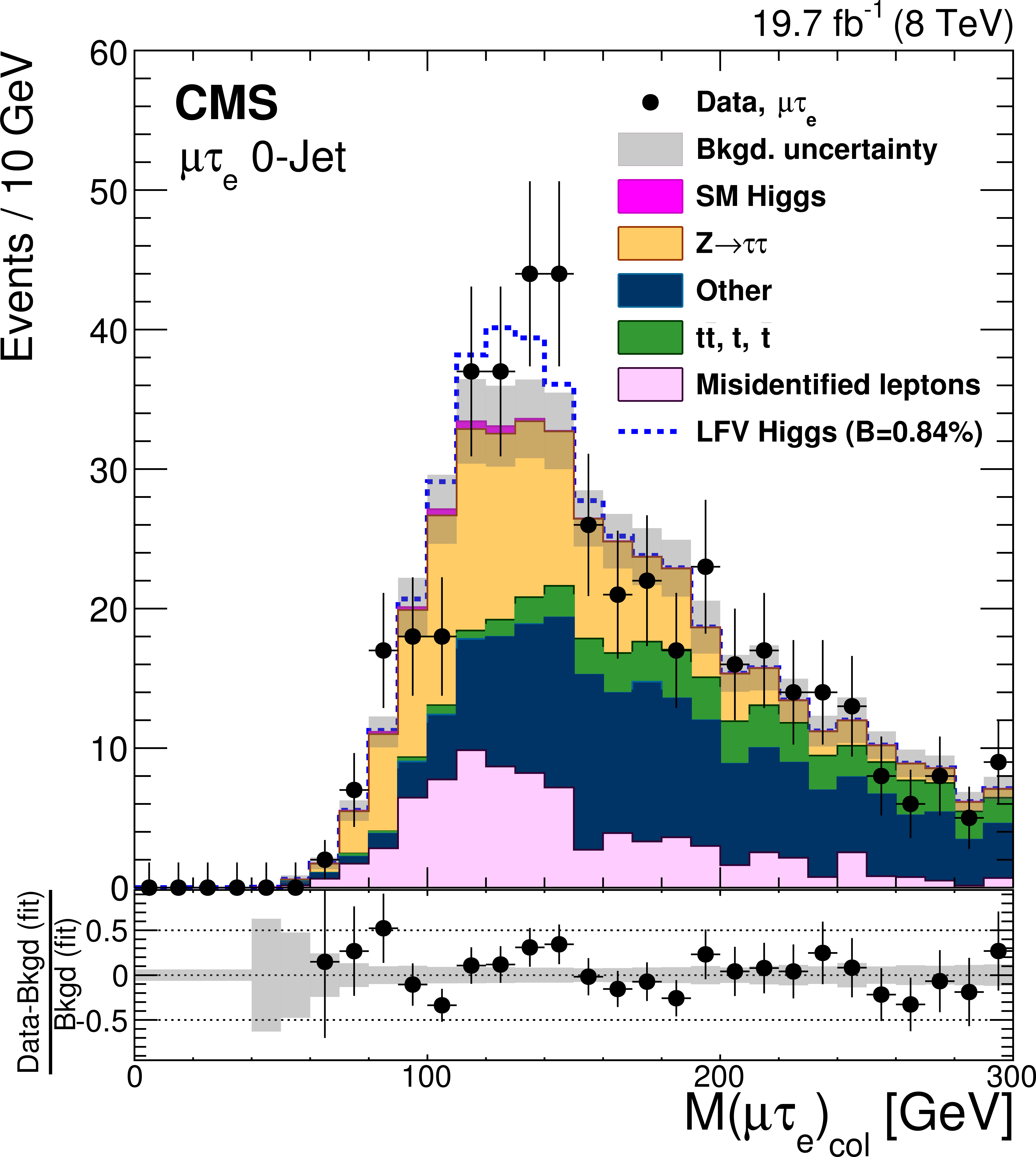
Figure 3-a:
Distributions of the collinear mass $M_\text {col}$ after fitting for signal and background for the LFV $ {\mathrm {H}} \to {{\mu }} {\tau }$ candidates in the different channels and categories compared to data. The bottom panel in each plot shows the fractional difference between the observed data and the fitted background. a: $ {\mathrm {H}} \to {{\mu }} {\tau }_{ {\mathrm {e}}}$ 0-jet; b: $ {\mathrm {H}} \to {{\mu }} { {\tau }_\mathrm {h}} $ 0-jet; c: $ {\mathrm {H}} \to {{\mu }} {\tau }_{ {\mathrm {e}}}$ 1-jet; d: $ {\mathrm {H}} \to {{\mu }} { {\tau }_\mathrm {h}} $ 1-jet; e: $ {\mathrm {H}} \to {{\mu }} {\tau }_{ {\mathrm {e}}}$ 2-jet; f: $ {\mathrm {H}} \to {{\mu }} { {\tau }_\mathrm {h}} $ 2-jet. |
png pdf |
Figure 3-b:
Distributions of the collinear mass $M_\text {col}$ after fitting for signal and background for the LFV $ {\mathrm {H}} \to {{\mu }} {\tau }$ candidates in the different channels and categories compared to data. The bottom panel in each plot shows the fractional difference between the observed data and the fitted background. a: $ {\mathrm {H}} \to {{\mu }} {\tau }_{ {\mathrm {e}}}$ 0-jet; b: $ {\mathrm {H}} \to {{\mu }} { {\tau }_\mathrm {h}} $ 0-jet; c: $ {\mathrm {H}} \to {{\mu }} {\tau }_{ {\mathrm {e}}}$ 1-jet; d: $ {\mathrm {H}} \to {{\mu }} { {\tau }_\mathrm {h}} $ 1-jet; e: $ {\mathrm {H}} \to {{\mu }} {\tau }_{ {\mathrm {e}}}$ 2-jet; f: $ {\mathrm {H}} \to {{\mu }} { {\tau }_\mathrm {h}} $ 2-jet. |
png pdf |
Figure 3-c:
Distributions of the collinear mass $M_\text {col}$ after fitting for signal and background for the LFV $ {\mathrm {H}} \to {{\mu }} {\tau }$ candidates in the different channels and categories compared to data. The bottom panel in each plot shows the fractional difference between the observed data and the fitted background. a: $ {\mathrm {H}} \to {{\mu }} {\tau }_{ {\mathrm {e}}}$ 0-jet; b: $ {\mathrm {H}} \to {{\mu }} { {\tau }_\mathrm {h}} $ 0-jet; c: $ {\mathrm {H}} \to {{\mu }} {\tau }_{ {\mathrm {e}}}$ 1-jet; d: $ {\mathrm {H}} \to {{\mu }} { {\tau }_\mathrm {h}} $ 1-jet; e: $ {\mathrm {H}} \to {{\mu }} {\tau }_{ {\mathrm {e}}}$ 2-jet; f: $ {\mathrm {H}} \to {{\mu }} { {\tau }_\mathrm {h}} $ 2-jet. |
png pdf |
Figure 3-d:
Distributions of the collinear mass $M_\text {col}$ after fitting for signal and background for the LFV $ {\mathrm {H}} \to {{\mu }} {\tau }$ candidates in the different channels and categories compared to data. The bottom panel in each plot shows the fractional difference between the observed data and the fitted background. a: $ {\mathrm {H}} \to {{\mu }} {\tau }_{ {\mathrm {e}}}$ 0-jet; b: $ {\mathrm {H}} \to {{\mu }} { {\tau }_\mathrm {h}} $ 0-jet; c: $ {\mathrm {H}} \to {{\mu }} {\tau }_{ {\mathrm {e}}}$ 1-jet; d: $ {\mathrm {H}} \to {{\mu }} { {\tau }_\mathrm {h}} $ 1-jet; e: $ {\mathrm {H}} \to {{\mu }} {\tau }_{ {\mathrm {e}}}$ 2-jet; f: $ {\mathrm {H}} \to {{\mu }} { {\tau }_\mathrm {h}} $ 2-jet. |

png pdf |
Figure 3-e:
Distributions of the collinear mass $M_\text {col}$ after fitting for signal and background for the LFV $ {\mathrm {H}} \to {{\mu }} {\tau }$ candidates in the different channels and categories compared to data. The bottom panel in each plot shows the fractional difference between the observed data and the fitted background. a: $ {\mathrm {H}} \to {{\mu }} {\tau }_{ {\mathrm {e}}}$ 0-jet; b: $ {\mathrm {H}} \to {{\mu }} { {\tau }_\mathrm {h}} $ 0-jet; c: $ {\mathrm {H}} \to {{\mu }} {\tau }_{ {\mathrm {e}}}$ 1-jet; d: $ {\mathrm {H}} \to {{\mu }} { {\tau }_\mathrm {h}} $ 1-jet; e: $ {\mathrm {H}} \to {{\mu }} {\tau }_{ {\mathrm {e}}}$ 2-jet; f: $ {\mathrm {H}} \to {{\mu }} { {\tau }_\mathrm {h}} $ 2-jet. |
png pdf |
Figure 3-f:
Distributions of the collinear mass $M_\text {col}$ after fitting for signal and background for the LFV $ {\mathrm {H}} \to {{\mu }} {\tau }$ candidates in the different channels and categories compared to data. The bottom panel in each plot shows the fractional difference between the observed data and the fitted background. a: $ {\mathrm {H}} \to {{\mu }} {\tau }_{ {\mathrm {e}}}$ 0-jet; b: $ {\mathrm {H}} \to {{\mu }} { {\tau }_\mathrm {h}} $ 0-jet; c: $ {\mathrm {H}} \to {{\mu }} {\tau }_{ {\mathrm {e}}}$ 1-jet; d: $ {\mathrm {H}} \to {{\mu }} { {\tau }_\mathrm {h}} $ 1-jet; e: $ {\mathrm {H}} \to {{\mu }} {\tau }_{ {\mathrm {e}}}$ 2-jet; f: $ {\mathrm {H}} \to {{\mu }} { {\tau }_\mathrm {h}} $ 2-jet. |
png pdf |
Figure 4-a:
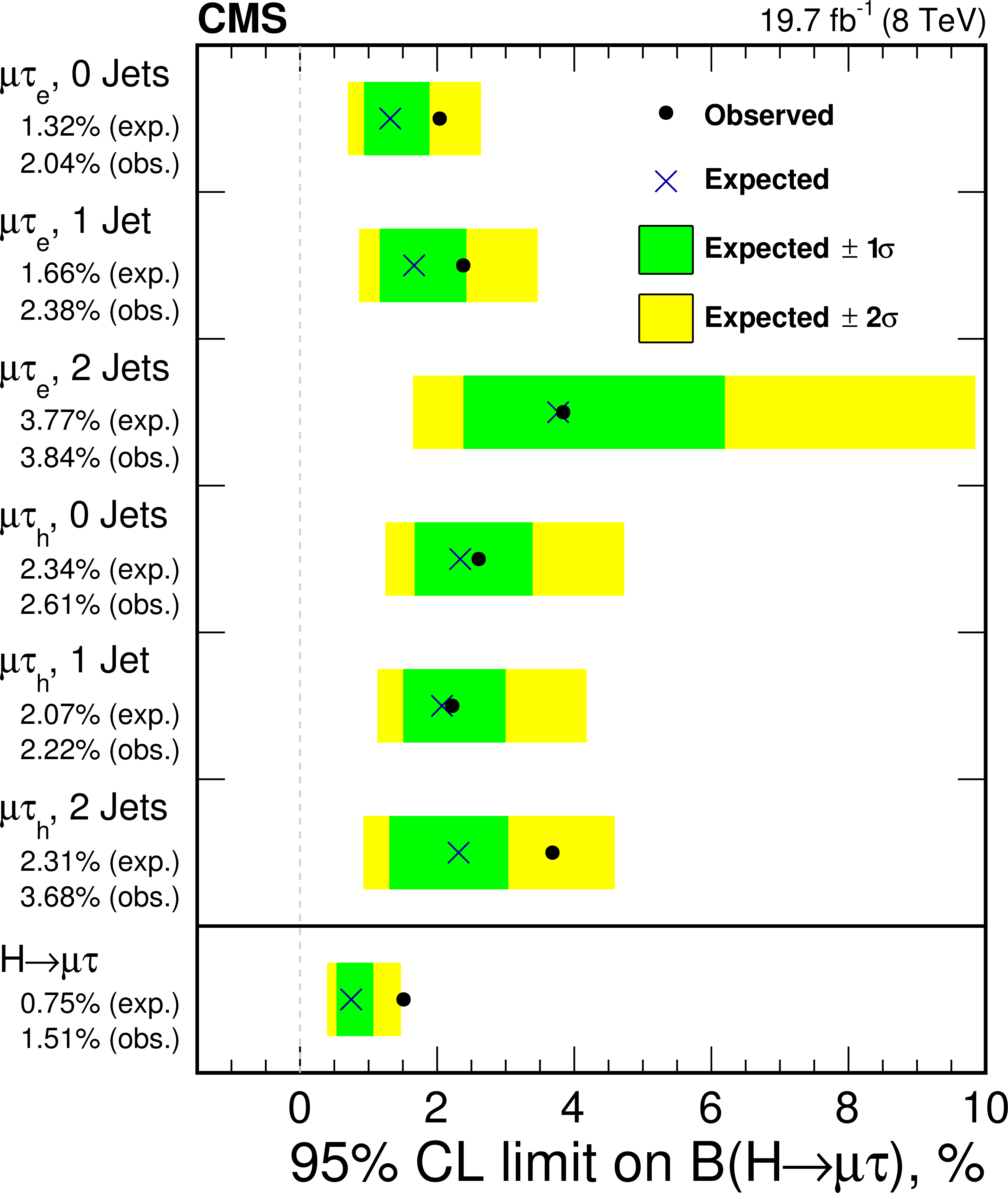
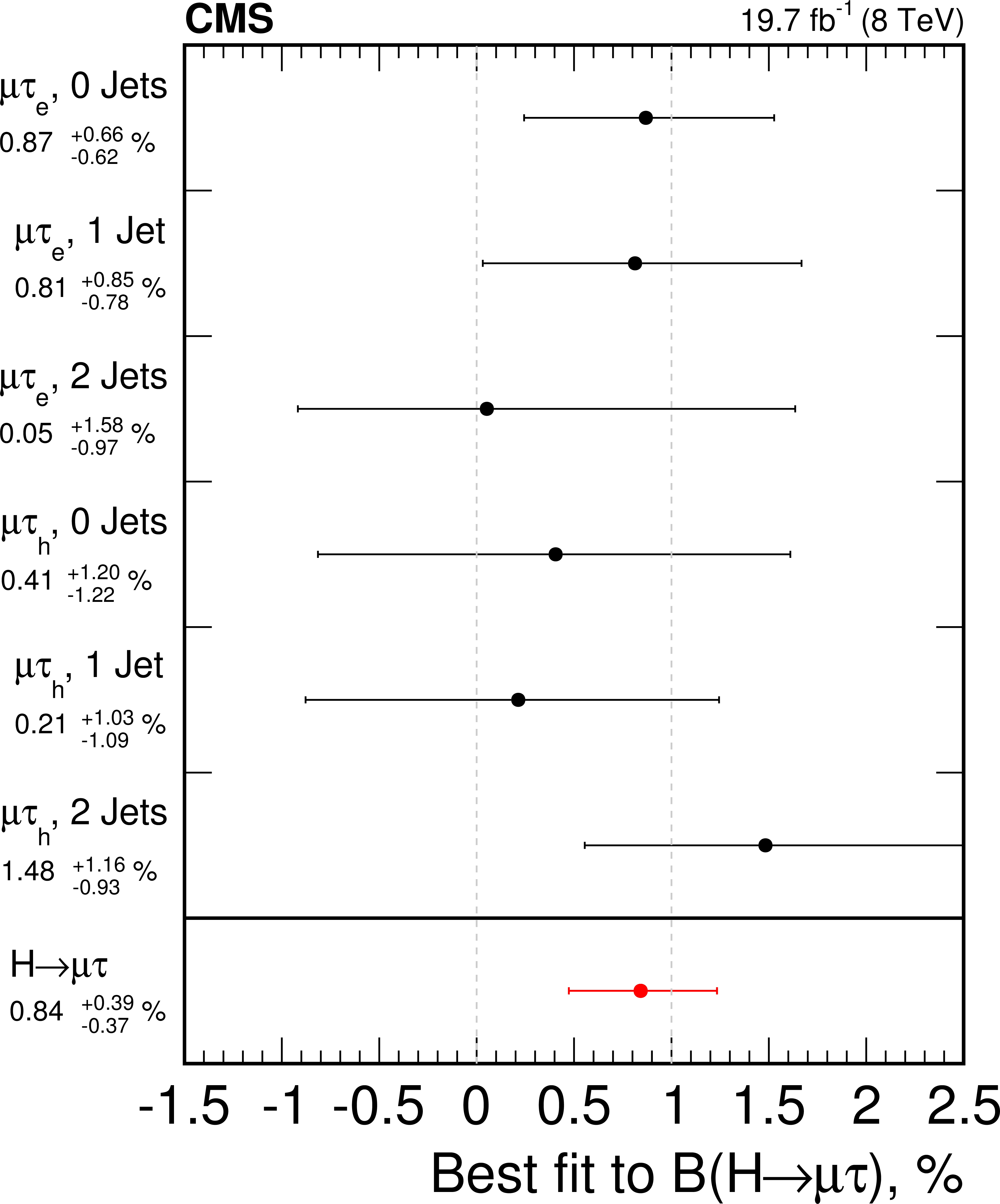
a: 95% CL Upper limits by category for the LFV $ {\mathrm {H}} \to {{\mu }} {\tau }$ decays. b: best fit branching fractions by category. |
png pdf |
Figure 4-b:
a: 95% CL Upper limits by category for the LFV $ {\mathrm {H}} \to {{\mu }} {\tau }$ decays. b: best fit branching fractions by category. |
png pdf |
Figure 5-a:
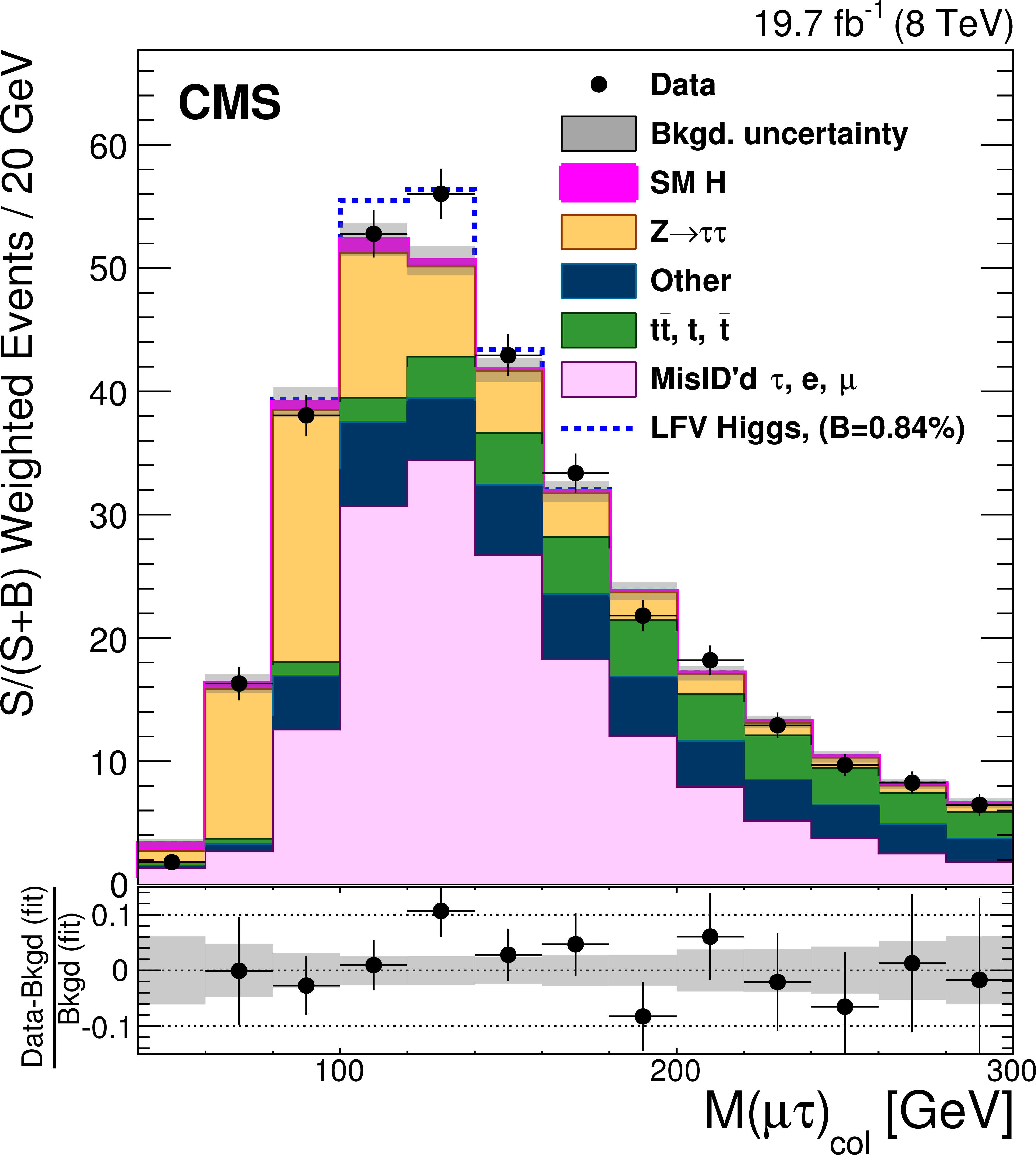
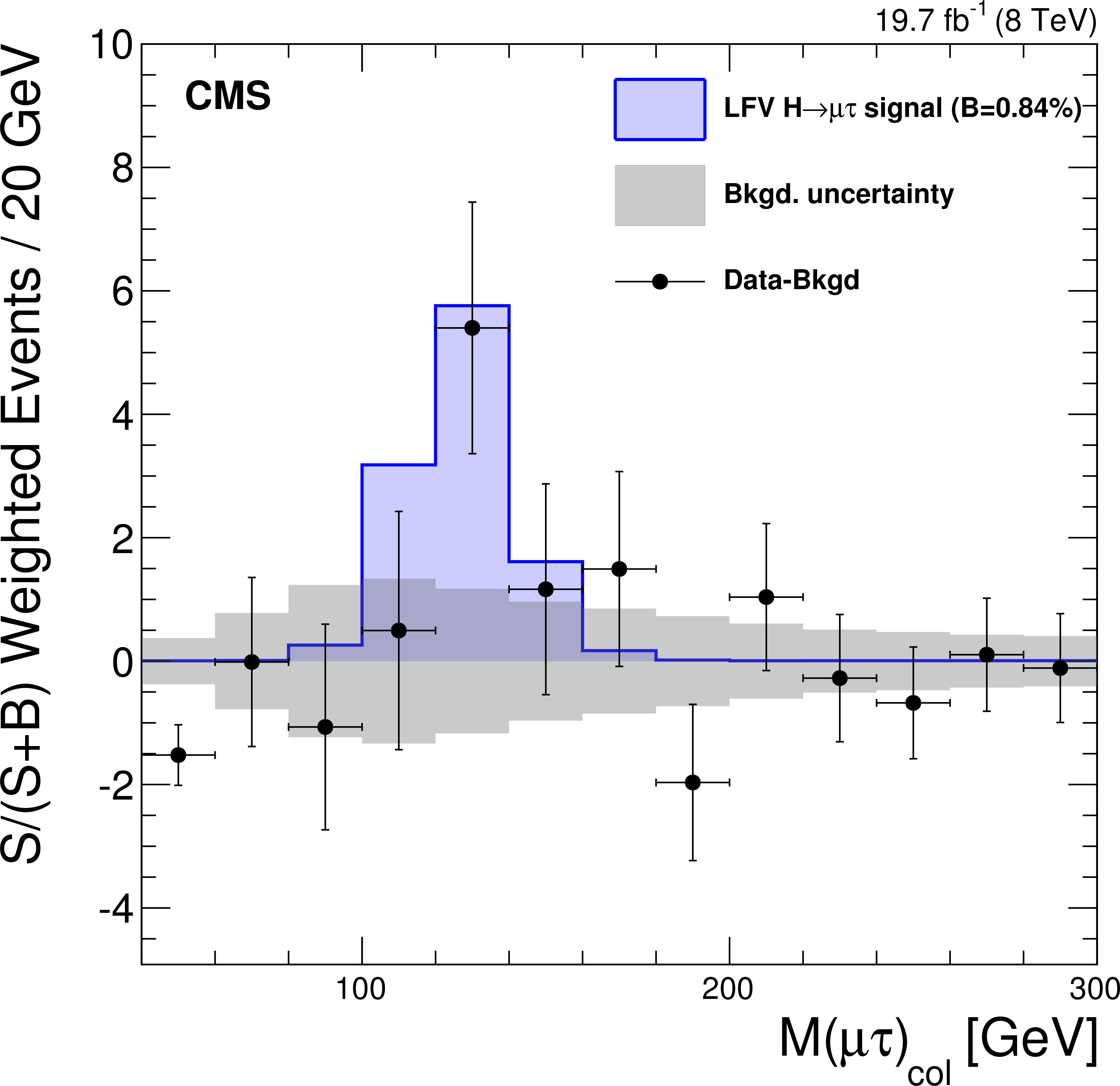
a: Distribution of $M_\text {col}$ for all categories combined, with each category weighted by significance ($\mathrm {S}/(\mathrm {S}+\mathrm {B})$). The significance is computed for the integral of the bins in the range 100 $< M_\text {col} <$ 150 GeV using $\mathcal {B}( {\mathrm {H}} \to {{\mu }} {\tau })=0.84%$. The MC Higgs signal shown is for $\mathcal {B}( {\mathrm {H}} \to {{\mu }} {\tau })=0.84%$. The bottom panel shows the fractional difference between the observed data and the fitted background. b: background subtracted $M_\text {col}$ distribution for all categories combined. |
png pdf |
Figure 5-b:
a: Distribution of $M_\text {col}$ for all categories combined, with each category weighted by significance ($\mathrm {S}/(\mathrm {S}+\mathrm {B})$). The significance is computed for the integral of the bins in the range 100 $< M_\text {col} <$ 150 GeV using $\mathcal {B}( {\mathrm {H}} \to {{\mu }} {\tau })=0.84%$. The MC Higgs signal shown is for $\mathcal {B}( {\mathrm {H}} \to {{\mu }} {\tau })=0.84%$. The bottom panel shows the fractional difference between the observed data and the fitted background. b: background subtracted $M_\text {col}$ distribution for all categories combined. |

png pdf |
Figure 6:
Constraints on the flavour-violating Yukawa couplings, $ {| Y_{ {{\mu }} {\tau }} | }$ and $ {| Y_{ {\tau } {{\mu }}} | }$. The black dashed lines are contours of $\mathcal {B}( {\mathrm {H}} \to {{\mu }} {\tau })$ for reference. The expected limit (red solid line) with one sigma (yellow) and two sigma (green) bands, and observed limit (black solid line) are derived from the limit on $\mathcal {B}( {\mathrm {H}} \to {{\mu }} {\tau })$ from the present analysis. The shaded regions are derived constraints from null searches for $ {\tau }\to 3 {{\mu }}$ (dark green) and $ {\tau }\to {{\mu }}\gamma $ (lighter green). The yellow line is the limit from a theoretical reinterpretation of an ATLAS $ {\mathrm {H}} \to {\tau } {\tau }$ search\cite {Harnik:2012pb}. The light blue region indicates the additional parameter space excluded by our result. The purple diagonal line is the theoretical naturalness limit $Y_{ij}Y_{ji} \leq m_im_j/v^2$. |
| Tables | |
png pdf |
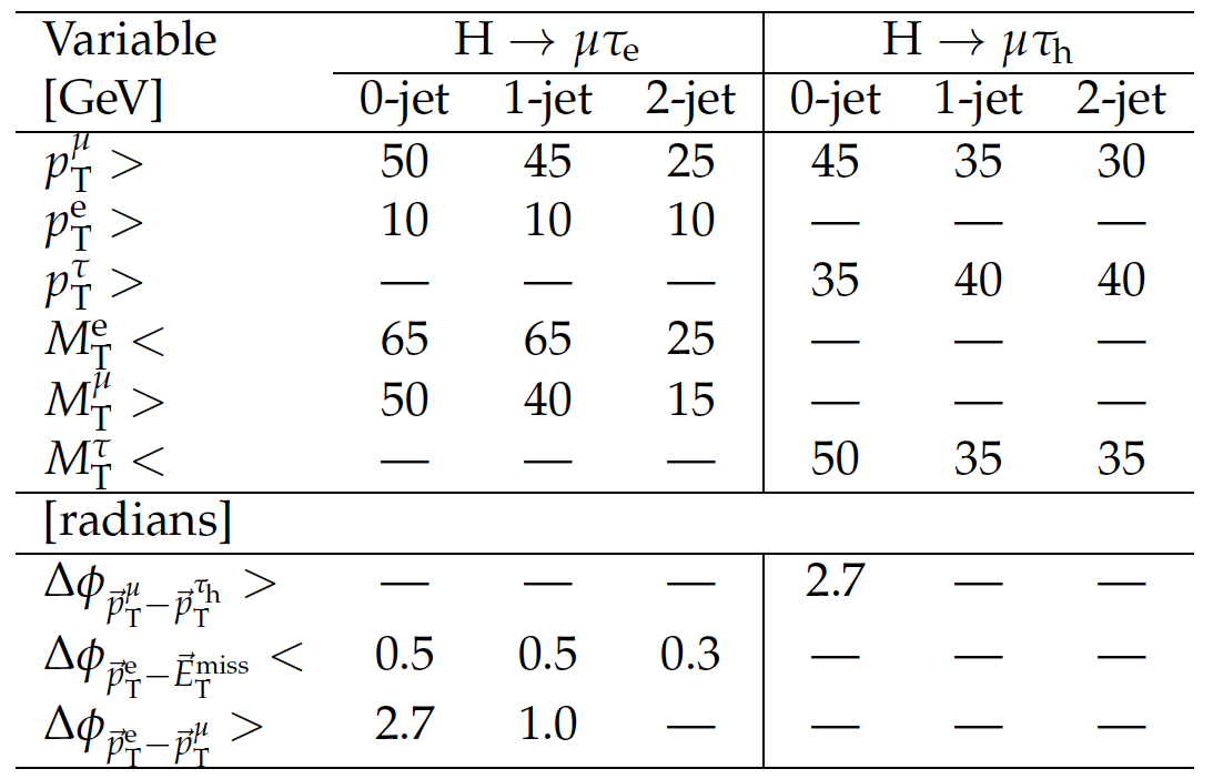
Table 1:
Selection criteria for the kinematic variables after the loose selection. |
png pdf |
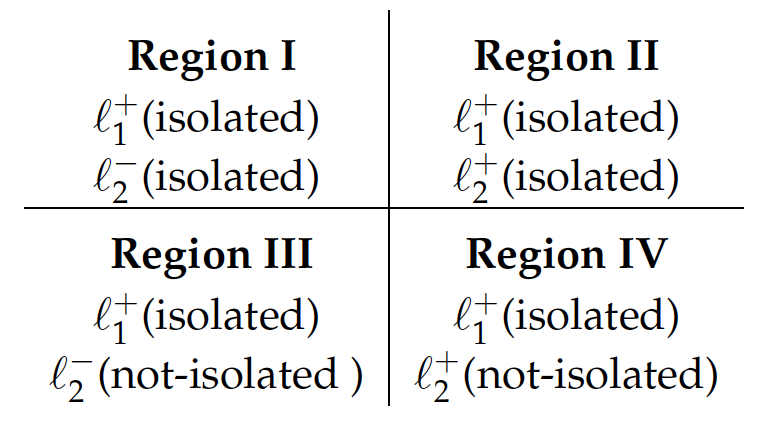
Table 2:
Schematic to illustrate the application of the method used to estimate the misidentified lepton ($\ell $) background. Samples are defined by the charge of the two leptons and by the isolation requirements on each. Charged conjugates are assumed. |
png pdf |
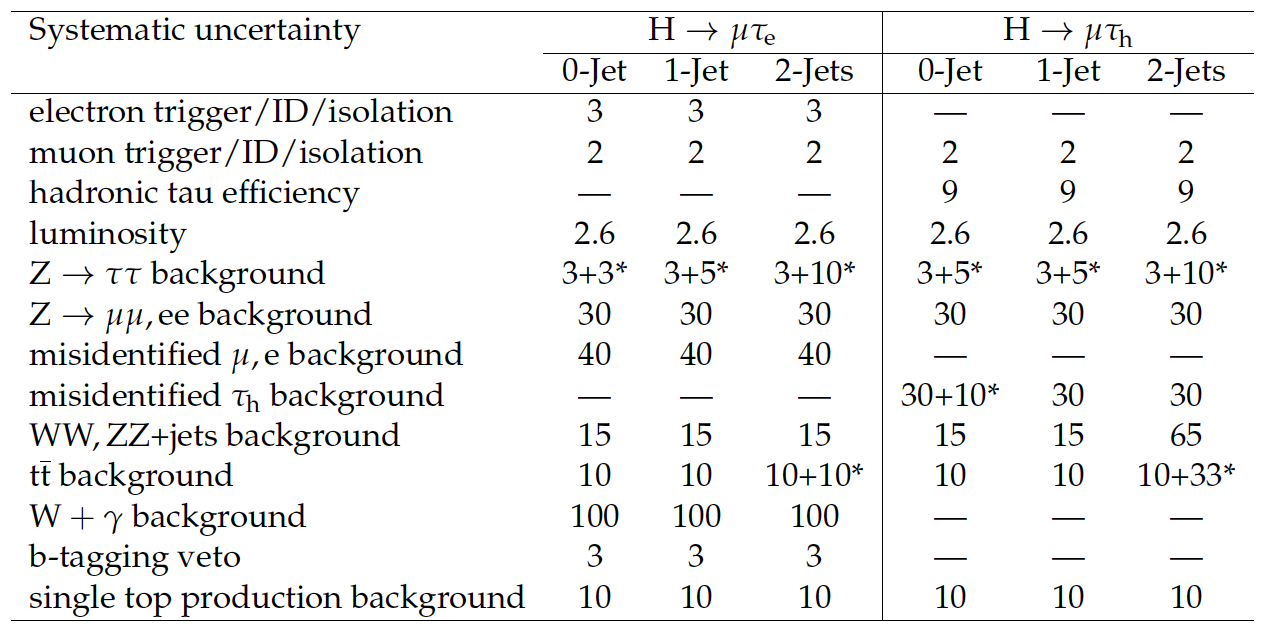
Table 3:
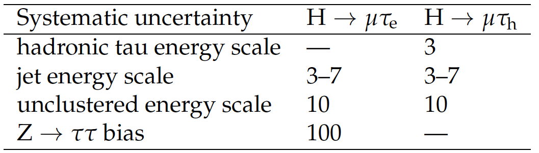
Systematic uncertainties in %. All uncertainties are treated as correlated between the categories, except where there are two numbers. In this case the number denoted with * is treated as uncorrelated between categories and the total uncertainty is the sum in quadrature of the two numbers. |
png pdf |
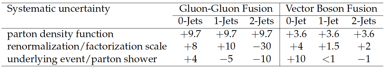
Table 4:
Theoretical uncertainties in % for Higgs boson production. Anticorrelations arise due to migration of events between the categories and are expressed as negative numbers. |
png pdf |
Table 5:
Systematic uncertainties in % for the shape of the signal and background templates. |
png pdf |
Table 6:
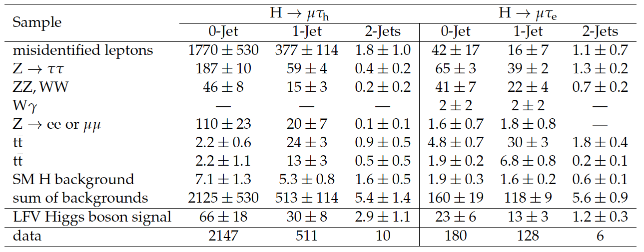
Event yields in the signal region, 100 $ < M_\text {col} < $ 150 GeV after fitting for signal and background. The expected contributions are normalized to an integrated luminosity of 19.7 fb$^{-1}$. The LFV Higgs boson signal is the expected yield for $B( {\mathrm {H}} \to \mu \tau ) = $ 0.84% with the SM Higgs boson cross section. |
png pdf |
Table 7:
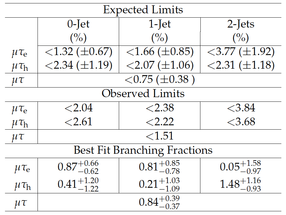
The expected upper limits, observed upper limits and best fit values for the branching fractions for different jet categories for the $ {\mathrm {H}} \to {{\mu }} {\tau }$ process. The one standard-deviation probability intervals around the expected limit are shown in parentheses. |
| Summary |
| The first direct search for lepton-flavour-violating decays of a Higgs boson to a $\mu \tau$ pair, based on the full 8 TeV data set collected by CMS in 2012 is presented. It improves upon previously published indirect limits [4, 26] by an order of magnitude. A slight excess of events with a significance of 2.4$\sigma$ is observed, corresponding to a $p$-value of 0.010. The best fit branching fraction is $ \cal{B} ( \mathrm{H} \to \mu \tau ) =$ (0.84 $\pm$ 0.39)%. A constraint of $ \cal{B} ( \mathrm{H} \to \mu \tau ) <$ 1.51% at 95% confidence level is set. The limit is used to constrain the Yukawa couplings, $ \sqrt{ | Y_{\mu\tau} |^2 + | Y_{\tau\mu} |^2 } < 3.6 \times 10^{-3}$. It improves the current bound by an order of magnitude. |
|
|
Compact Muon Solenoid LHC, CERN |
|

|

|

|

|

|