

Compact Muon Solenoid
LHC, CERN
| CMS-HIG-14-009 ; CERN-PH-EP-2014-288 | ||
| Precise determination of the mass of the Higgs boson and tests of compatibility of its couplings with the standard model predictions using proton collisions at 7 and 8 TeV | ||
| CMS Collaboration | ||
| 30 December 2014 | ||
| Eur. Phys. J. C 75 (2015) 212 | ||
|
Abstract:
Properties of the Higgs boson with mass near 125 GeV are measured in proton-proton collisions with the CMS experiment at the LHC. Comprehensive sets of production and decay measurements are combined. The decay channels include $ \gamma \gamma$, ZZ, WW, $ \tau \tau$, bb, and $ \mu \mu$ pairs. The data samples were collected in 2011 and 2012 and correspond to integrated luminosities of up to 5.1 fb$ ^{-1} $ at 7 TeV and up to 19.7 fb$ ^{-1} $ at 8 TeV. From the high-resolution $ \gamma \gamma $ and ZZ channels, the mass of the Higgs boson is determined to be $m_{\mathrm{H}}$ = 125.02 $ ^{+0.26}_{-0.27} $ (stat) $ ^{+0.14}_{-0.15}$ (syst) GeV. For this mass value, the event yields obtained in the different analyses tagging specific decay channels and production mechanisms are consistent with those expected for the standard model Higgs boson. The combined best-fit signal relative to the standard model expectation is 1.00 $\pm$ 0.09(stat) $ ^{+0.08}_{-0.07}$ (theo) $\pm$ 0.07(syst) at the measured mass. The couplings of the Higgs boson are probed for deviations in magnitude from the standard model predictions in multiple ways, including searches for invisible and undetected decays. No significant deviations are found. | ||
| Links: e-print arXiv:1412.8662 [hep-ex] (PDF) ; CDS record ; inSPIRE record ; Public twiki page ; CADI line (restricted) ; | ||
| Cover | |
png ; pdf |
Cover of European Physics Journal C, volume 75, number 5, May 2015. |
| Figures | |

png pdf |
Figure 1:
The 68% CL confidence regions for the signal strength $\sigma / \sigma _{\text {SM}}$ versus the mass of the boson $ {\mathrm {m}_{ {\mathrm {H}} }} $ for the ${ {\mathrm {H}} \to { {\gamma } {\gamma } } } $ and ${ { {\mathrm {H}} \to { {\mathrm {Z}} {\mathrm {Z}}} } \to 4\ell } $ final states, and their combination. The symbol $\sigma / \sigma _{\text {SM}}$ denotes the production cross section times the relevant branching fractions, relative to the SM expectation. In this combination, the relative signal strength for the two decay modes is set to the expectation for the SM Higgs boson. |
png pdf |
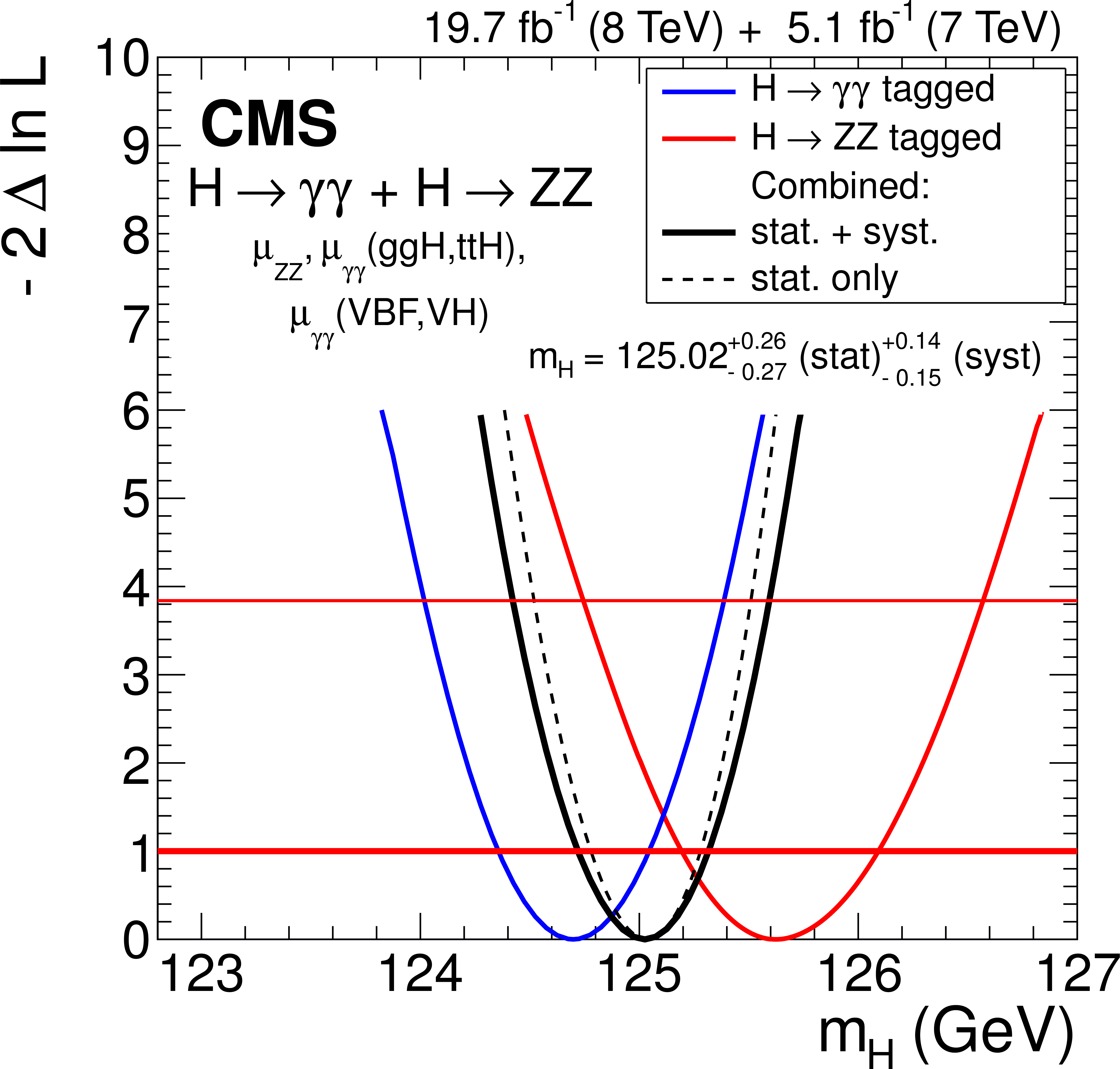
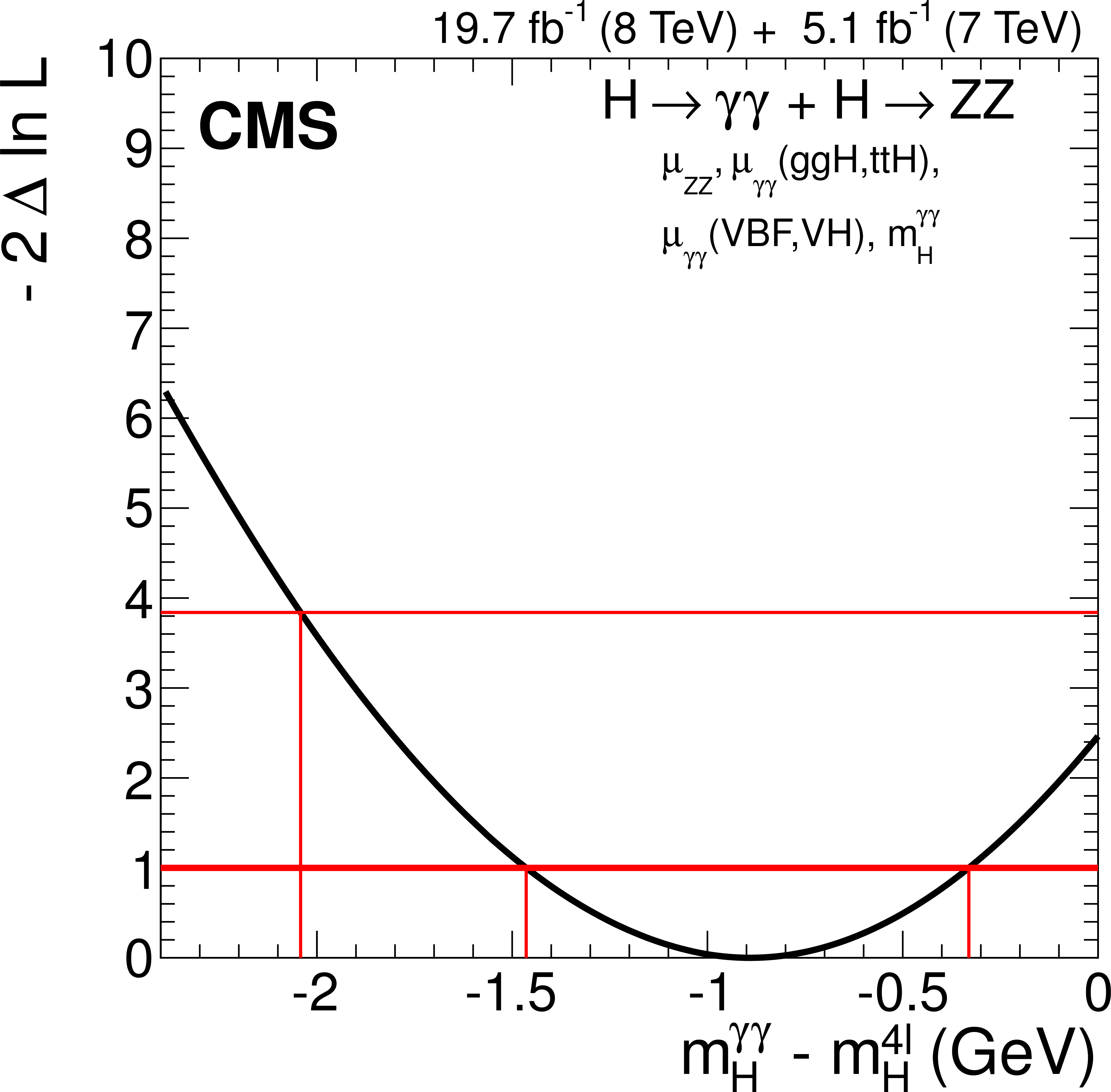
Figure 2-a:
(a) Scan of the test statistic $q( {m_\mathrm { {\mathrm {H}} }} )=-2 \Delta \ln\mathcal {L} $ versus the mass of the boson $ {m_\mathrm { {\mathrm {H}} }} $ for the ${ {\mathrm {H}} \to { {\gamma } {\gamma } } }$ and ${ { {\mathrm {H}} \to { {\mathrm {Z}} {\mathrm {Z}}} } \to 4\ell } $ final states separately and for their combination. Three independent signal strengths, $( { {\mathrm {g}} {\mathrm {g}} {\mathrm {H}} } , { {\mathrm {t}} {\mathrm {t}} {\mathrm {H}} } )\to { {\gamma } {\gamma } } $, $( {\mathrm {VBF}} , {\mathrm {V} {\mathrm {H}} } )\to { {\gamma } {\gamma } } $, and $\text {pp}\to { { {\mathrm {H}} \to { {\mathrm {Z}} {\mathrm {Z}}} } \to 4\ell } $, are profiled together with all other nuisance parameters. (b) Scan of the test statistic $q(m_{ {\mathrm {H}} }^{ { {\gamma } {\gamma } } } - m_{ {\mathrm {H}} }^{4\ell })$ versus the difference between two individual mass measurements for the same model of signal strengths used in the left panel. |
png pdf |
Figure 2-b:
(a) Scan of the test statistic $q( {m_\mathrm { {\mathrm {H}} }} )=-2 \Delta \ln\mathcal {L} $ versus the mass of the boson $ {m_\mathrm { {\mathrm {H}} }} $ for the ${ {\mathrm {H}} \to { {\gamma } {\gamma } } }$ and ${ { {\mathrm {H}} \to { {\mathrm {Z}} {\mathrm {Z}}} } \to 4\ell } $ final states separately and for their combination. Three independent signal strengths, $( { {\mathrm {g}} {\mathrm {g}} {\mathrm {H}} } , { {\mathrm {t}} {\mathrm {t}} {\mathrm {H}} } )\to { {\gamma } {\gamma } } $, $( {\mathrm {VBF}} , {\mathrm {V} {\mathrm {H}} } )\to { {\gamma } {\gamma } } $, and $\text {pp}\to { { {\mathrm {H}} \to { {\mathrm {Z}} {\mathrm {Z}}} } \to 4\ell } $, are profiled together with all other nuisance parameters. (b) Scan of the test statistic $q(m_{ {\mathrm {H}} }^{ { {\gamma } {\gamma } } } - m_{ {\mathrm {H}} }^{4\ell })$ versus the difference between two individual mass measurements for the same model of signal strengths used in the left panel. |
png pdf |
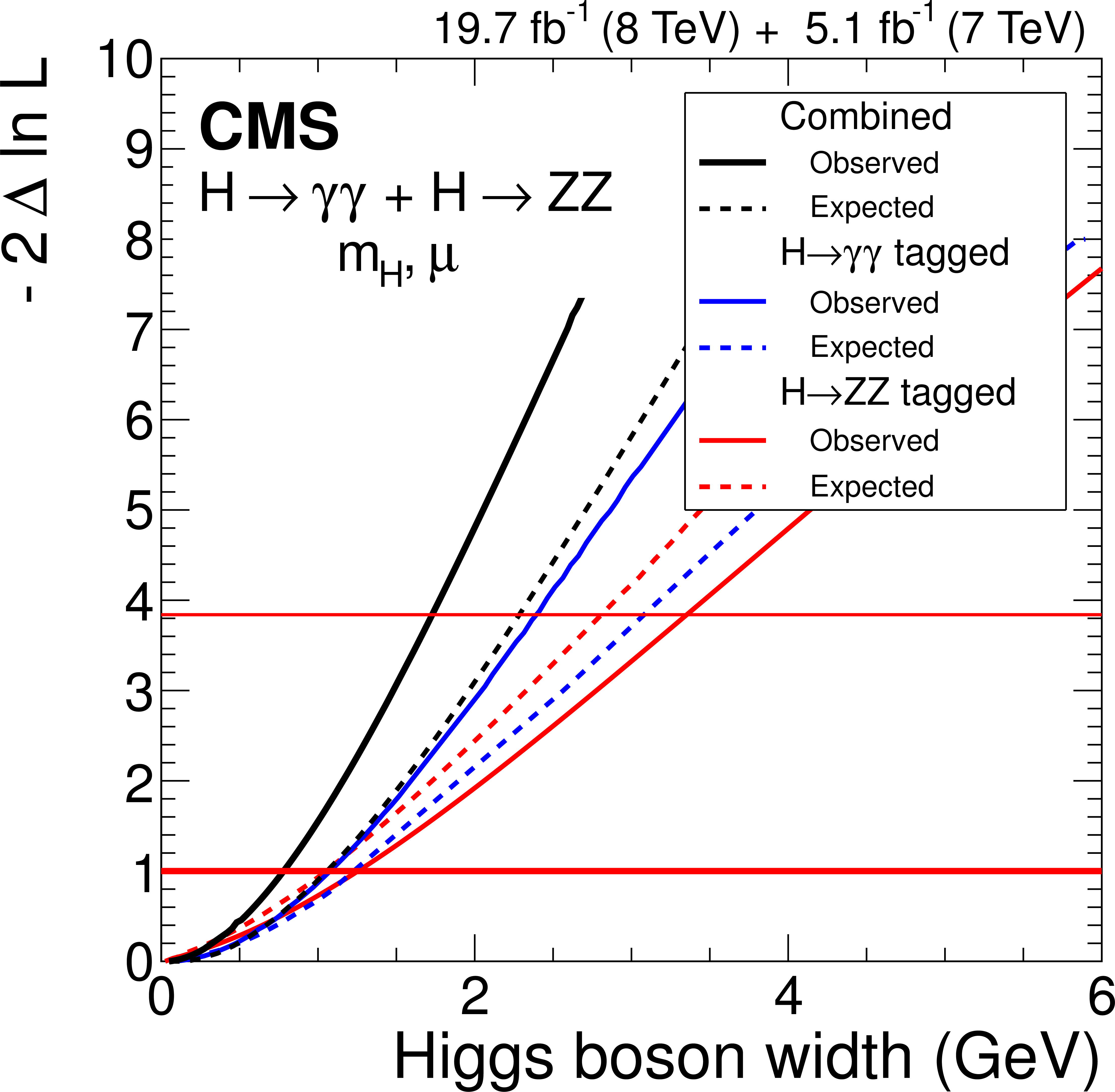
Figure 3:
Likelihood scan as a function of the width of the boson. The continuous (dashed) lines show the observed (expected) results for the ${ {\mathrm {H}} \to { {\gamma } {\gamma } } } $ analysis, the $ { { {\mathrm {H}} \to { {\mathrm {Z}} {\mathrm {Z}}} } \to 4\ell } $ analysis, and their combination. The data are consistent with $ {\Gamma _\mathrm {SM}} \sim$ 4 MeV and for the combination of the two channels the observed (expected) upper limit on the width at the 95% CL is 1.7 (2.3 ) GeV. |

png pdf |
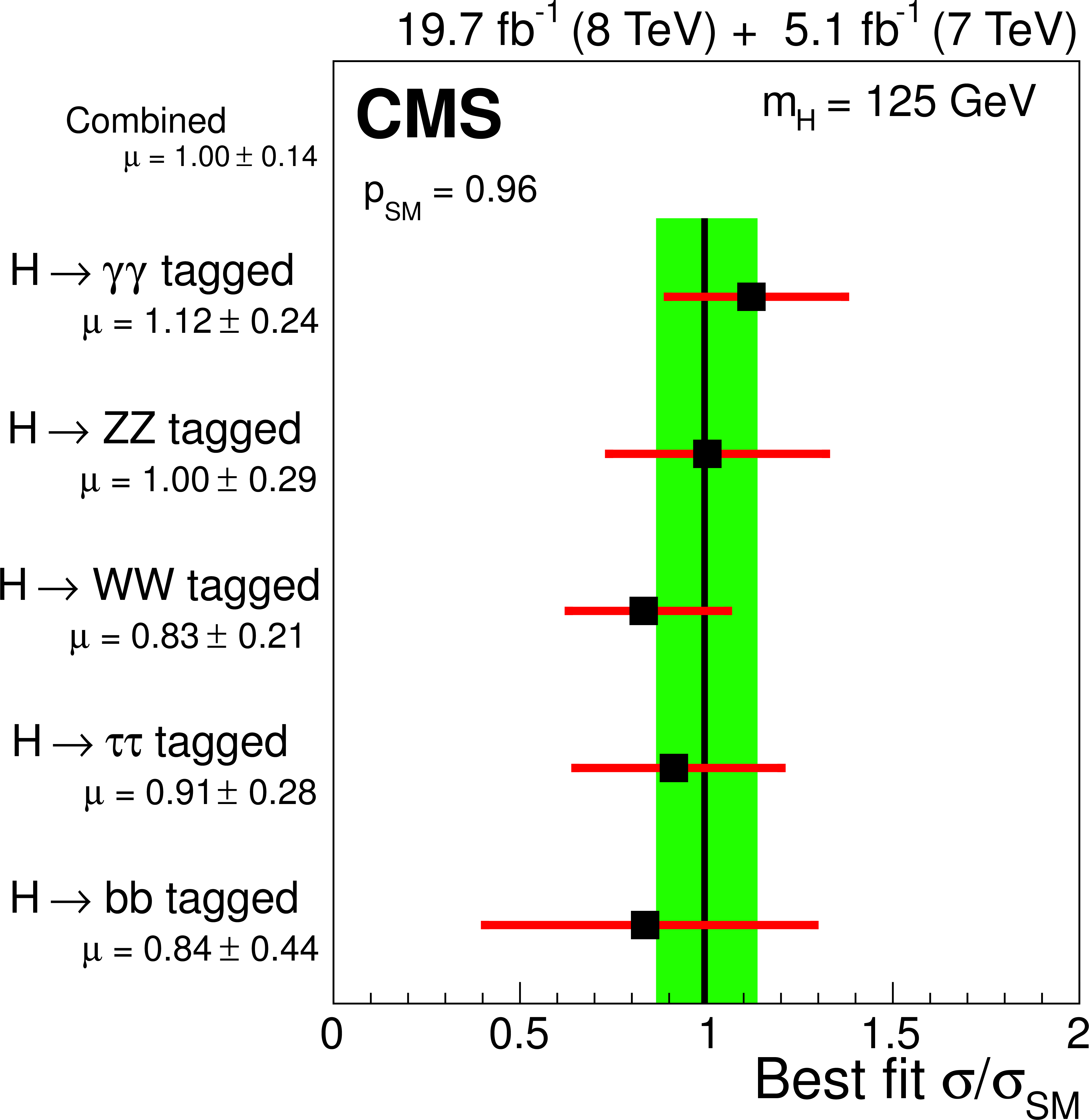
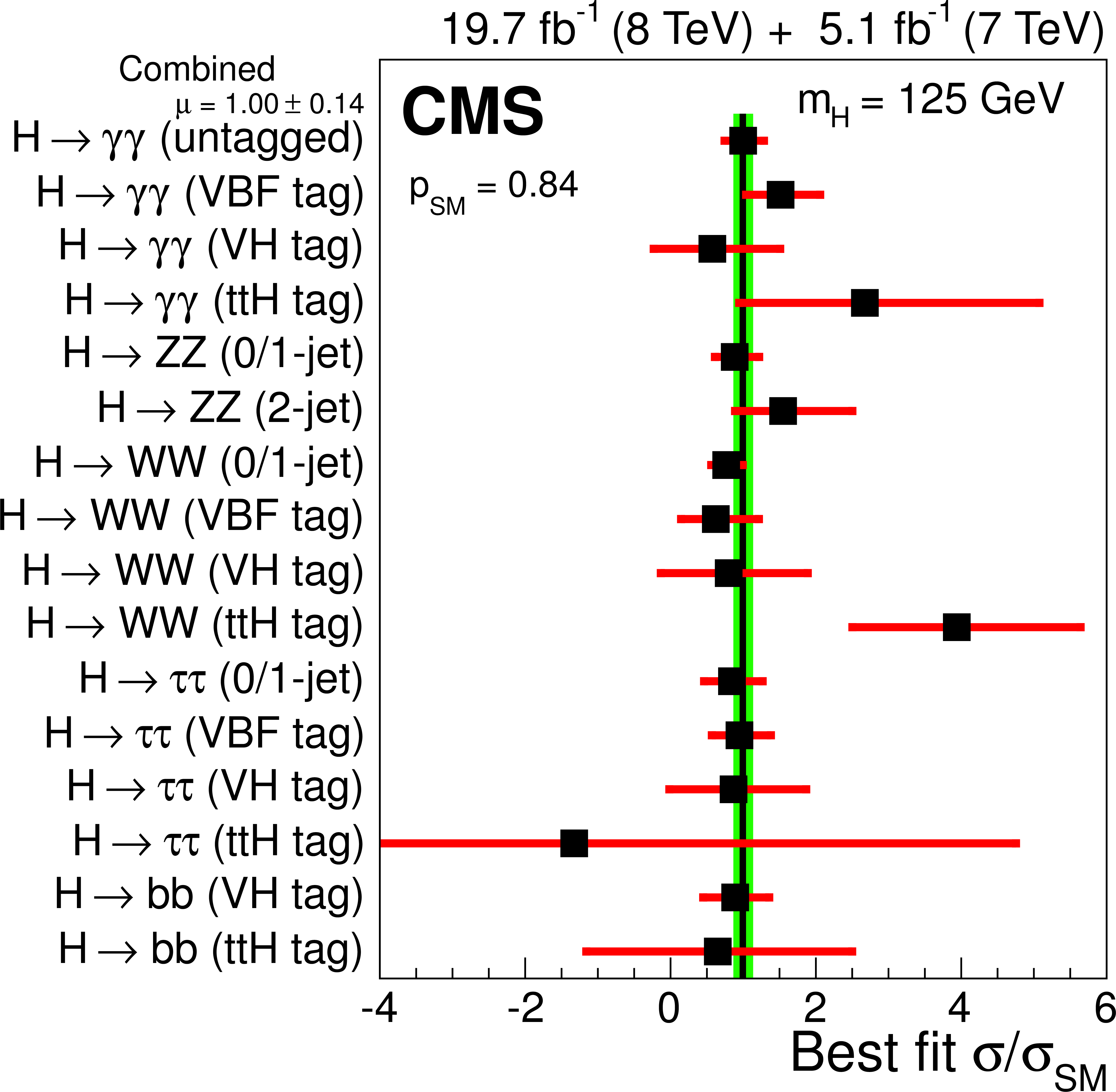
Figure 4-a:
Values of the best-fit $\sigma / \sigma _\text {SM}$ for the overall combined analysis (solid vertical line) and separate combinations grouped by production mode tag, predominant decay mode, or both. The $\sigma / \sigma _{\text {SM}}$ ratio denotes the production cross section times the relevant branching fractions, relative to the SM expectation. The vertical band shows the overall $\sigma / \sigma _\text {SM}$ uncertainty. The horizontal bars indicate the $\pm 1 $ standard deviation uncertainties in the best-fit $\sigma / \sigma _\text {SM}$ values for the individual combinations; these bars include both statistical and systematic uncertainties. (a) Combinations grouped by analysis tags targeting individual production mechanisms; the excess in the $ { {\mathrm {t}} {\mathrm {t}} {\mathrm {H}} } $-tagged combination is largely driven by the ${ {\mathrm {t}} {\mathrm {t}} {\mathrm {H}} } $-tagged ${ {\mathrm {H}} \to { {\gamma } {\gamma } } } $ and $ { {\mathrm {H}} \to { {\mathrm {W}} {\mathrm {W}}} } $ channels as can be seen in the bottom panel. (b) Combinations grouped by predominant decay mode. (c) Combinations grouped by predominant decay mode and additional tags targeting a particular production mechanism. |
png pdf |
Figure 4-b:
Values of the best-fit $\sigma / \sigma _\text {SM}$ for the overall combined analysis (solid vertical line) and separate combinations grouped by production mode tag, predominant decay mode, or both. The $\sigma / \sigma _{\text {SM}}$ ratio denotes the production cross section times the relevant branching fractions, relative to the SM expectation. The vertical band shows the overall $\sigma / \sigma _\text {SM}$ uncertainty. The horizontal bars indicate the $\pm 1 $ standard deviation uncertainties in the best-fit $\sigma / \sigma _\text {SM}$ values for the individual combinations; these bars include both statistical and systematic uncertainties. (a) Combinations grouped by analysis tags targeting individual production mechanisms; the excess in the $ { {\mathrm {t}} {\mathrm {t}} {\mathrm {H}} } $-tagged combination is largely driven by the ${ {\mathrm {t}} {\mathrm {t}} {\mathrm {H}} } $-tagged ${ {\mathrm {H}} \to { {\gamma } {\gamma } } } $ and $ { {\mathrm {H}} \to { {\mathrm {W}} {\mathrm {W}}} } $ channels as can be seen in the bottom panel. (b) Combinations grouped by predominant decay mode. (c) Combinations grouped by predominant decay mode and additional tags targeting a particular production mechanism. |
png pdf |
Figure 4-c:
Values of the best-fit $\sigma / \sigma _\text {SM}$ for the overall combined analysis (solid vertical line) and separate combinations grouped by production mode tag, predominant decay mode, or both. The $\sigma / \sigma _{\text {SM}}$ ratio denotes the production cross section times the relevant branching fractions, relative to the SM expectation. The vertical band shows the overall $\sigma / \sigma _\text {SM}$ uncertainty. The horizontal bars indicate the $\pm 1 $ standard deviation uncertainties in the best-fit $\sigma / \sigma _\text {SM}$ values for the individual combinations; these bars include both statistical and systematic uncertainties. (a) Combinations grouped by analysis tags targeting individual production mechanisms; the excess in the $ { {\mathrm {t}} {\mathrm {t}} {\mathrm {H}} } $-tagged combination is largely driven by the ${ {\mathrm {t}} {\mathrm {t}} {\mathrm {H}} } $-tagged ${ {\mathrm {H}} \to { {\gamma } {\gamma } } } $ and $ { {\mathrm {H}} \to { {\mathrm {W}} {\mathrm {W}}} } $ channels as can be seen in the bottom panel. (b) Combinations grouped by predominant decay mode. (c) Combinations grouped by predominant decay mode and additional tags targeting a particular production mechanism. |

png pdf |
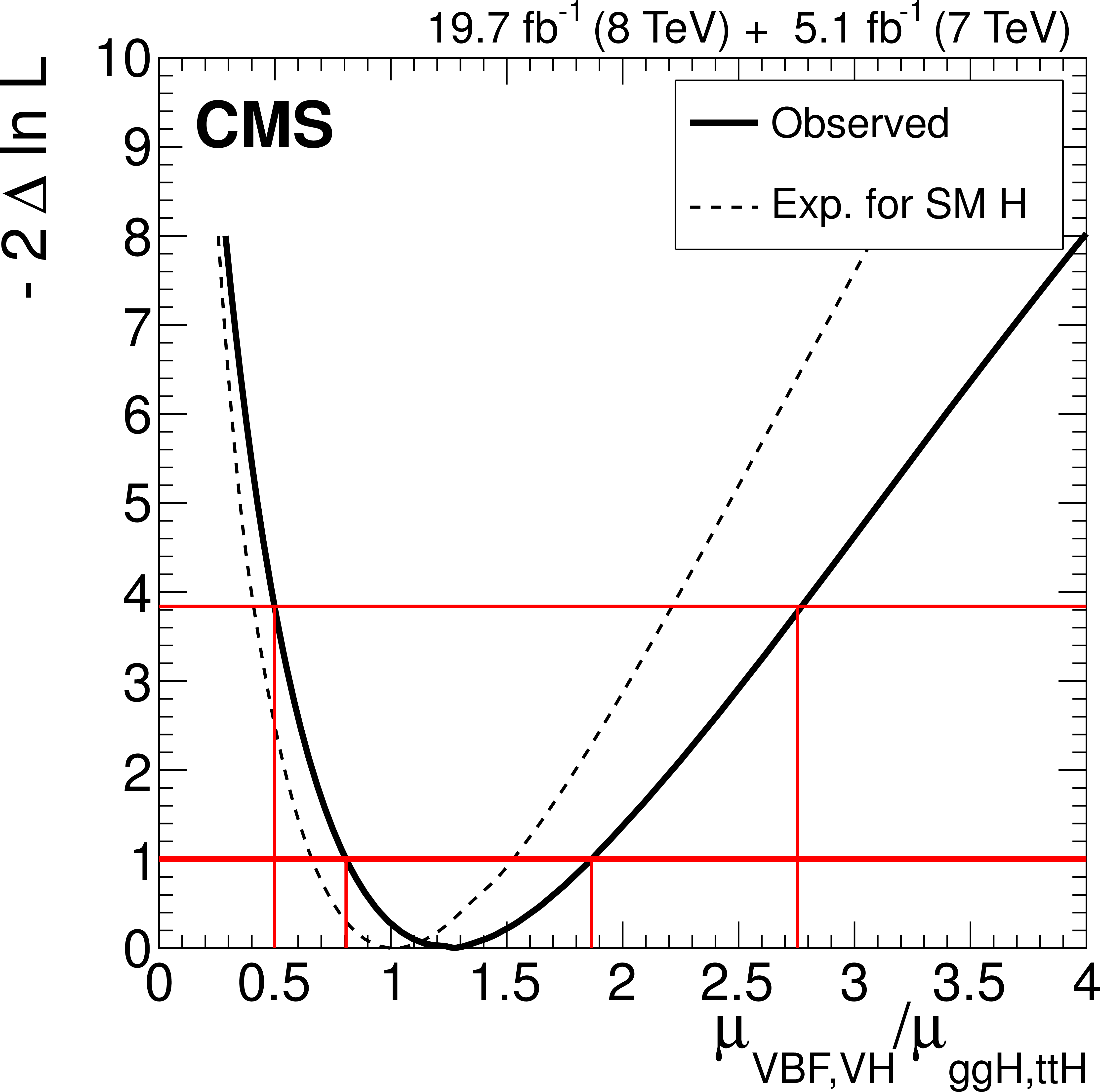
Figure 5-a:
(a) The 68% CL confidence regions (bounded by the solid curves) for the signal strength of the ggH and ttH and of the VBF and VH production mechanisms, $ {\mu _{ { {\mathrm {g}} {\mathrm {g}} {\mathrm {H}} } , { {\mathrm {t}} {\mathrm {t}} {\mathrm {H}} } }} $ and ${\mu _{ {\mathrm {VBF}} , {\mathrm {V} {\mathrm {H}} } }} $, respectively. The crosses indicate the best-fit values obtained in each group of predominant decay modes: $ { {\gamma } {\gamma } } $, ${ {\mathrm {Z}} {\mathrm {Z}}} $, $ { {\mathrm {W}} {\mathrm {W}}} $, ${ {\tau } {\tau } } $, and ${ {\mathrm {b}} {\mathrm {b}} } $. The diamond at $(1,1)$ indicates the expected values for the SM Higgs boson. (b) Likelihood scan versus the ratio $ { {\mu _{ {\mathrm {VBF}} , {\mathrm {V} {\mathrm {H}} } }} / {\mu _{ { {\mathrm {g}} {\mathrm {g}} {\mathrm {H}} } , { {\mathrm {t}} {\mathrm {t}} {\mathrm {H}} } }} } $, combined for all channels. The fit for ${ {\mu _{ {\mathrm {VBF}} , {\mathrm {V} {\mathrm {H}} } }} / {\mu _{ { {\mathrm {g}} {\mathrm {g}} {\mathrm {H}} } , { {\mathrm {t}} {\mathrm {t}} {\mathrm {H}} } }} } $ is performed while profiling the five $ {\mu _{ { {\mathrm {g}} {\mathrm {g}} {\mathrm {H}} } , { {\mathrm {t}} {\mathrm {t}} {\mathrm {H}} } }} $ parameters, one per visible decay mode, as shown in Table 4. The solid curve represents the observed result in data while the dashed curve indicates the expected median result in the presence of the SM Higgs boson. Crossings with the horizontal thick and thin lines denote the 68% CL and 95% CL confidence intervals, respectively. |
png pdf |
Figure 5-b:
(a) The 68% CL confidence regions (bounded by the solid curves) for the signal strength of the ggH and ttH and of the VBF and VH production mechanisms, $ {\mu _{ { {\mathrm {g}} {\mathrm {g}} {\mathrm {H}} } , { {\mathrm {t}} {\mathrm {t}} {\mathrm {H}} } }} $ and ${\mu _{ {\mathrm {VBF}} , {\mathrm {V} {\mathrm {H}} } }} $, respectively. The crosses indicate the best-fit values obtained in each group of predominant decay modes: $ { {\gamma } {\gamma } } $, ${ {\mathrm {Z}} {\mathrm {Z}}} $, $ { {\mathrm {W}} {\mathrm {W}}} $, ${ {\tau } {\tau } } $, and ${ {\mathrm {b}} {\mathrm {b}} } $. The diamond at $(1,1)$ indicates the expected values for the SM Higgs boson. (b) Likelihood scan versus the ratio $ { {\mu _{ {\mathrm {VBF}} , {\mathrm {V} {\mathrm {H}} } }} / {\mu _{ { {\mathrm {g}} {\mathrm {g}} {\mathrm {H}} } , { {\mathrm {t}} {\mathrm {t}} {\mathrm {H}} } }} } $, combined for all channels. The fit for ${ {\mu _{ {\mathrm {VBF}} , {\mathrm {V} {\mathrm {H}} } }} / {\mu _{ { {\mathrm {g}} {\mathrm {g}} {\mathrm {H}} } , { {\mathrm {t}} {\mathrm {t}} {\mathrm {H}} } }} } $ is performed while profiling the five $ {\mu _{ { {\mathrm {g}} {\mathrm {g}} {\mathrm {H}} } , { {\mathrm {t}} {\mathrm {t}} {\mathrm {H}} } }} $ parameters, one per visible decay mode, as shown in Table 4. The solid curve represents the observed result in data while the dashed curve indicates the expected median result in the presence of the SM Higgs boson. Crossings with the horizontal thick and thin lines denote the 68% CL and 95% CL confidence intervals, respectively. |
png pdf |
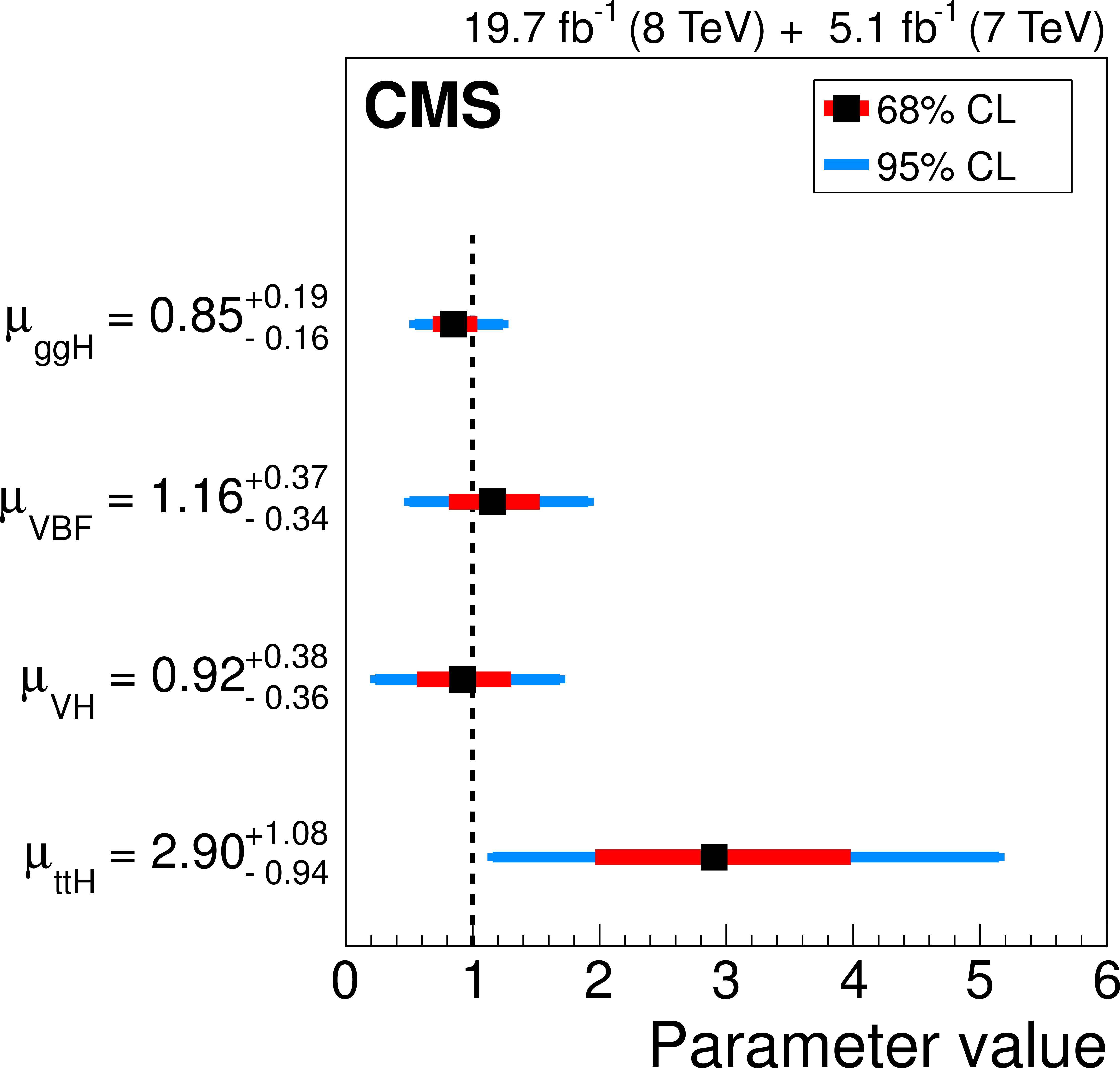
Figure 6:
Likelihood scan results for $ {\mu _{ { {\mathrm {g}} {\mathrm {g}} {\mathrm {H}} } }} , {\mu _{ {\mathrm {VBF}} }} $, $ {\mu _{ {\mathrm {V} {\mathrm {H}} } }} $, and $ {\mu _{ { {\mathrm {t}} {\mathrm {t}} {\mathrm {H}} } }} $. The inner bars represent the 68% CL confidence intervals while the outer bars represent the 95% CL confidence intervals. When scanning each individual parameter, the three other parameters are profiled. The SM values of the relative branching fractions are assumed for the different decay modes. |
png pdf |
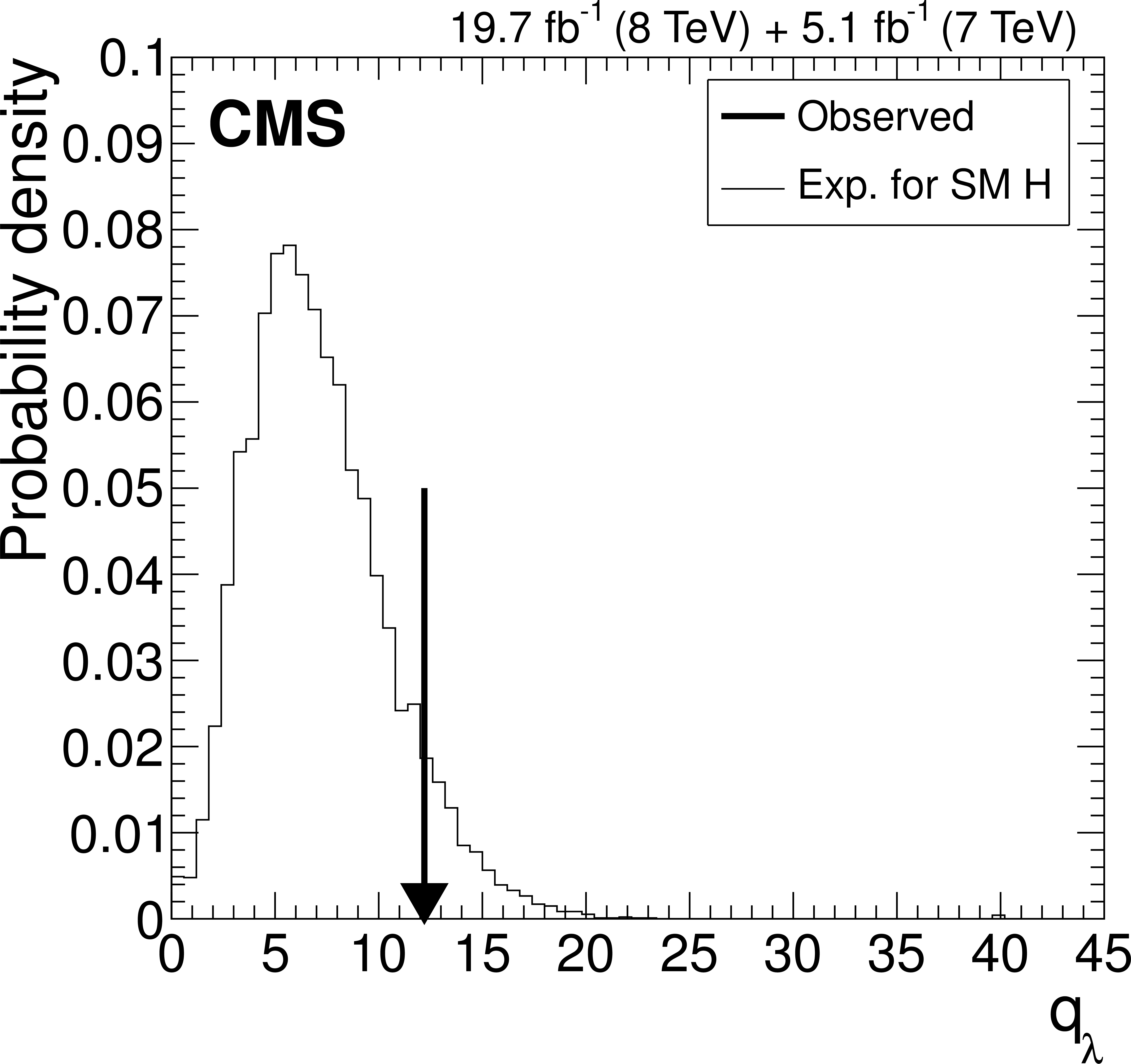
Figure 7:
Distribution of the profile likelihood ratio $q_\lambda $ between different assumptions for the structure of the matrix of signal strengths for the production processes and decay modes both for pseudo-data samples generated under the SM hypothesis and the value observed in data. The likelihood in the numerator is that for the data under a model of a general rank 1 matrix, expected if the observations are due to a single particle and of which the SM is a particular case. The likelihood in the denominator is that for the data under a ``saturated model'' with as many parameters as there are matrix elements. The arrow represents the observed value in data, $q_\lambda ^\text {obs}$. Under the SM hypothesis, the probability to find a value of $q_\lambda \geq q_\lambda ^\text {obs}$ is (7.9 $\pm$ 0.3)%, where the uncertainty reflects only the finite number of pseudo-data samples generated. |

png pdf |
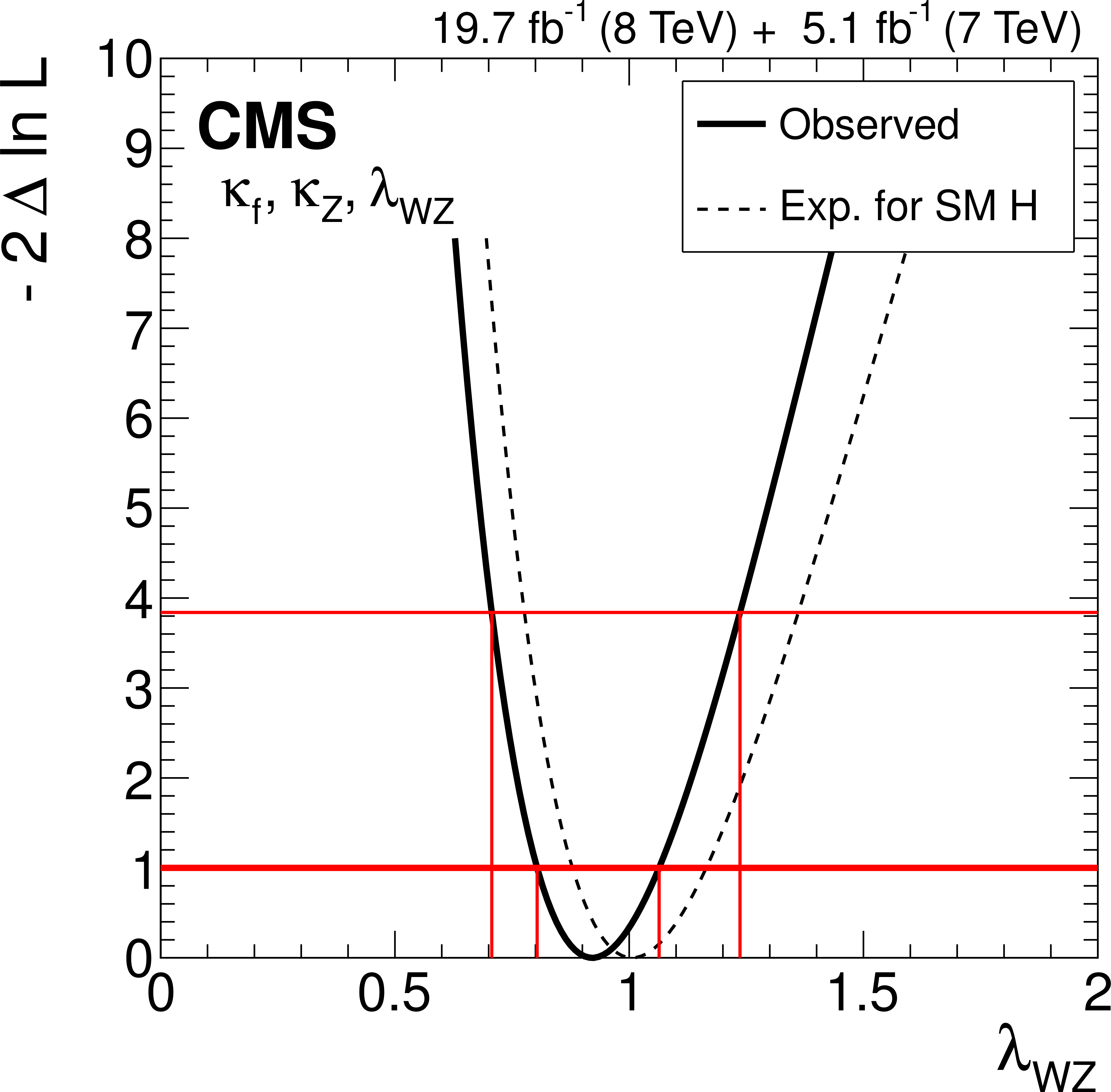
Figure 8-a:
Likelihood scans versus $ {\lambda _{\mathrm { {\mathrm {W}} {\mathrm {Z}}}}} $, the ratio of the coupling scaling factors to $ {\mathrm {W}}$ and $ {\mathrm {Z}}$ bosons: (left) from untagged $\text {pp} \to { {\mathrm {H}} \to { {\mathrm {W}} {\mathrm {W}}} } $ and $\text {pp} \to { {\mathrm {H}} \to { {\mathrm {Z}} {\mathrm {Z}}} } $ searches, assuming the SM couplings to fermions, $ {\kappa _{\mathrm {f}}} =1$; (right) from the combination of all channels, profiling the coupling to fermions. The solid curve represents the observation in data. The dashed curve indicates the expected median result in the presence of the SM Higgs boson. Crossings with the horizontal thick and thin lines denote the 68% CL and 95% CL confidence intervals, respectively. |
png pdf |
Figure 8-b:
Likelihood scans versus $ {\lambda _{\mathrm { {\mathrm {W}} {\mathrm {Z}}}}} $, the ratio of the coupling scaling factors to $ {\mathrm {W}}$ and $ {\mathrm {Z}}$ bosons: (left) from untagged $\text {pp} \to { {\mathrm {H}} \to { {\mathrm {W}} {\mathrm {W}}} } $ and $\text {pp} \to { {\mathrm {H}} \to { {\mathrm {Z}} {\mathrm {Z}}} } $ searches, assuming the SM couplings to fermions, $ {\kappa _{\mathrm {f}}} =1$; (right) from the combination of all channels, profiling the coupling to fermions. The solid curve represents the observation in data. The dashed curve indicates the expected median result in the presence of the SM Higgs boson. Crossings with the horizontal thick and thin lines denote the 68% CL and 95% CL confidence intervals, respectively. |
png pdf |
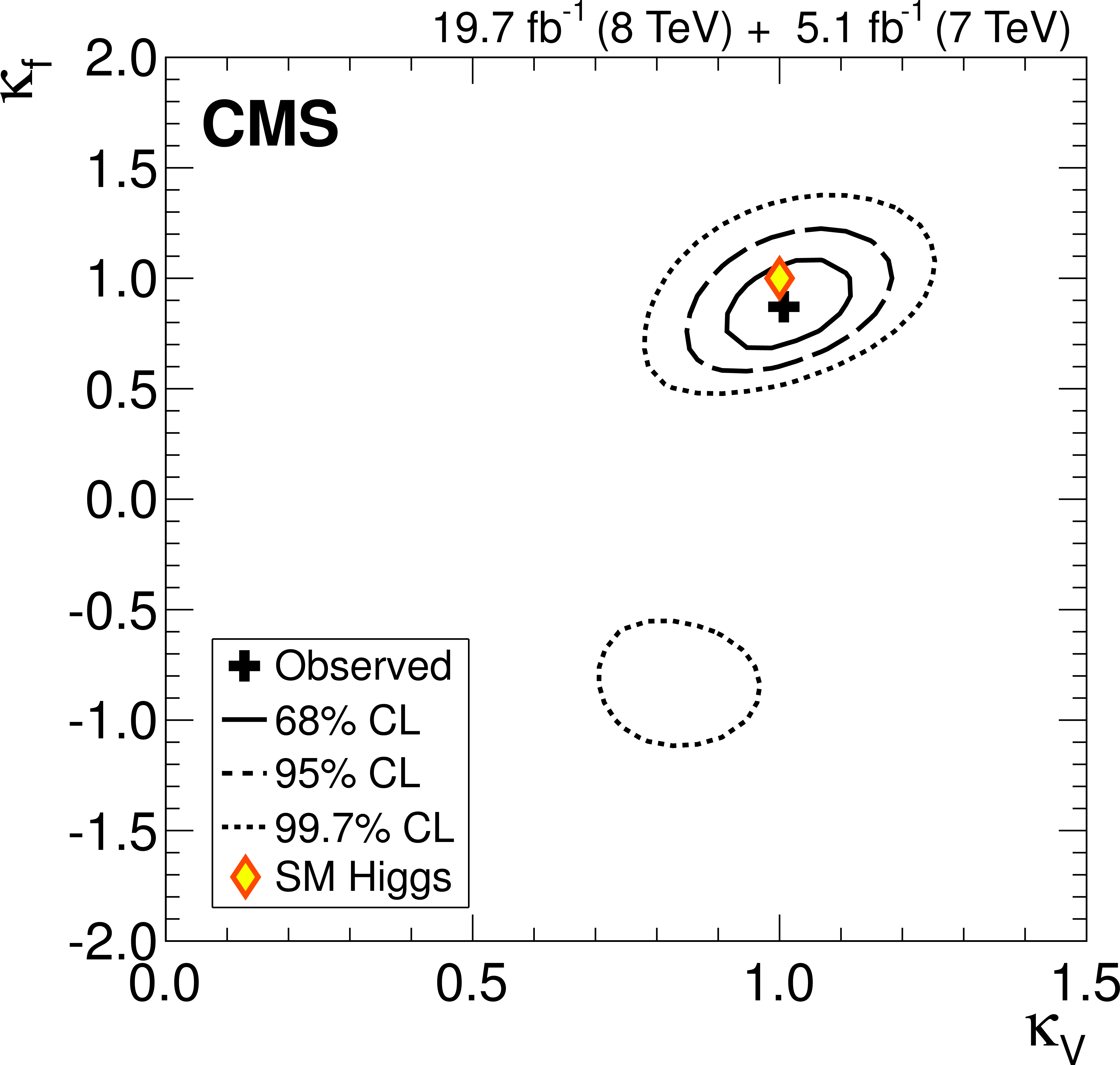
Figure 9-a:
Results of 2D likelihood scans for the $ {\kappa _{\mathrm {V}}} $ and $ {\kappa _{\mathrm {f}}} $ parameters. The cross indicates the best-fit values. The solid, dashed, and dotted contours show the 68%, 95%, and 99.7% CL confidence regions, respectively. The diamond shows the SM point $( {\kappa _{\mathrm {V}}} , {\kappa _{\mathrm {f}}} )=(1,1)$. The left plot shows the likelihood scan in two quadrants, $(+,+)$ and $(+,-)$. The right plot shows the likelihood scan constrained to the $(+,+)$ quadrant. |
png pdf |
Figure 9-b:
Results of 2D likelihood scans for the $ {\kappa _{\mathrm {V}}} $ and $ {\kappa _{\mathrm {f}}} $ parameters. The cross indicates the best-fit values. The solid, dashed, and dotted contours show the 68%, 95%, and 99.7% CL confidence regions, respectively. The diamond shows the SM point $( {\kappa _{\mathrm {V}}} , {\kappa _{\mathrm {f}}} )=(1,1)$. The left plot shows the likelihood scan in two quadrants, $(+,+)$ and $(+,-)$. The right plot shows the likelihood scan constrained to the $(+,+)$ quadrant. |

png pdf |
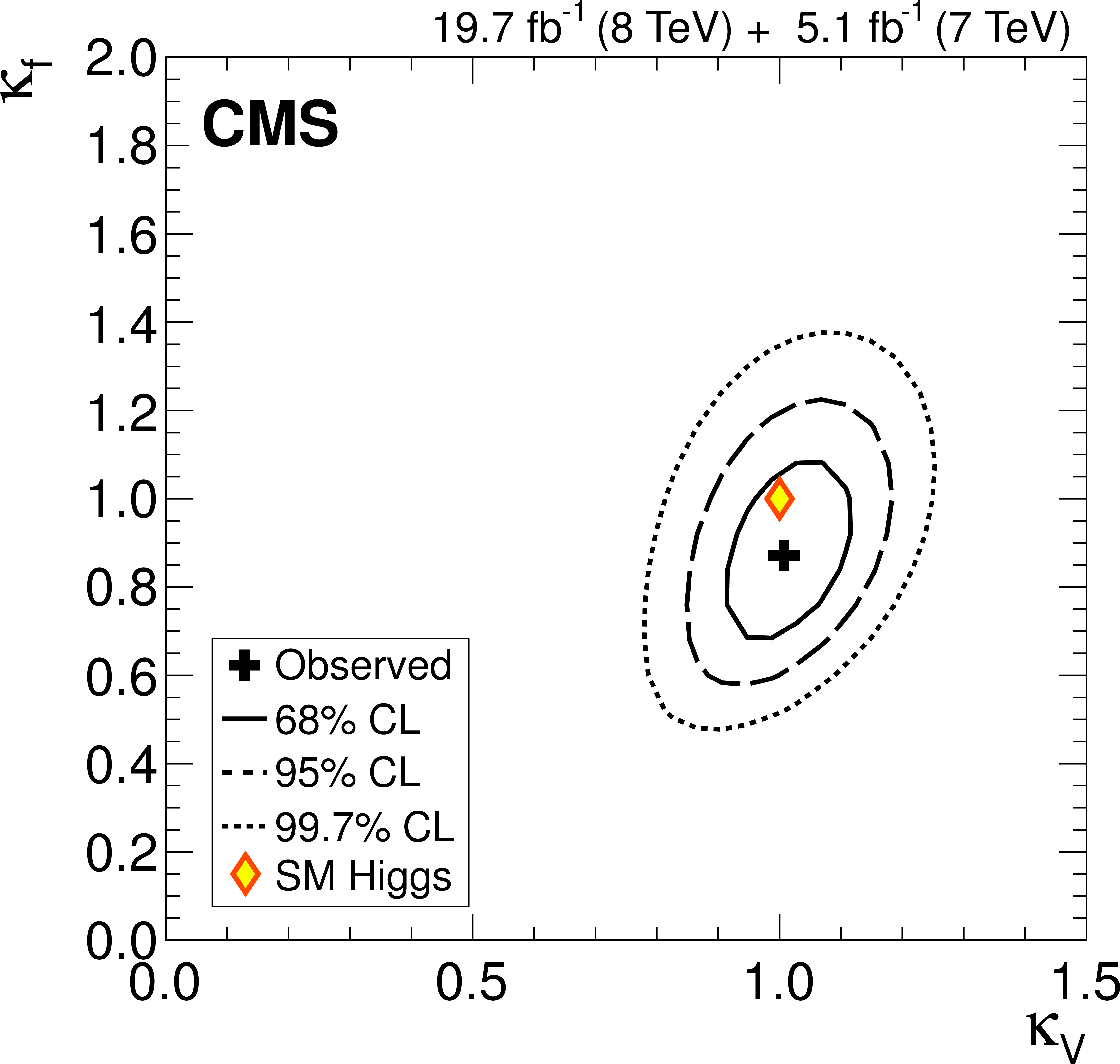
Figure 10-a:
The 68% CL confidence regions for individual channels (coloured swaths) and for the overall combination (thick curve) for the $ {\kappa _{\mathrm {V}}} $ and $ {\kappa _{\mathrm {f}}} $ parameters. The cross indicates the global best-fit values. The dashed contour bounds the 95% CL confidence region for the combination. The diamond represents the SM expectation, $( {\kappa _{\mathrm {V}}} , {\kappa _{\mathrm {f}}} )=(1,1)$. The left plot shows the likelihood scan in two quadrants $(+,+)$ and $(+,-)$, the right plot shows the positive quadrant only. |
png pdf |
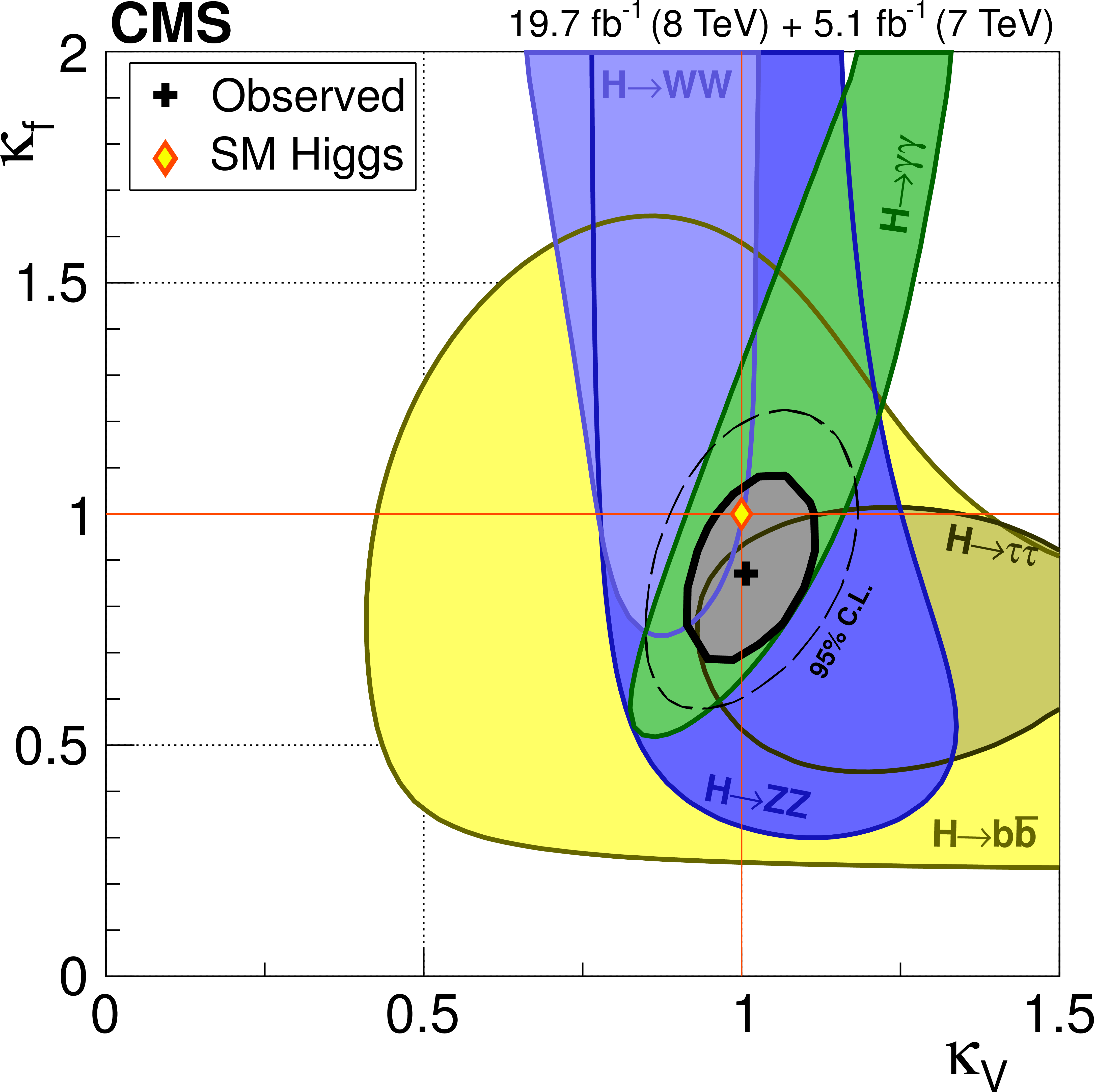
Figure 10-b:
The 68% CL confidence regions for individual channels (coloured swaths) and for the overall combination (thick curve) for the $ {\kappa _{\mathrm {V}}} $ and $ {\kappa _{\mathrm {f}}} $ parameters. The cross indicates the global best-fit values. The dashed contour bounds the 95% CL confidence region for the combination. The diamond represents the SM expectation, $( {\kappa _{\mathrm {V}}} , {\kappa _{\mathrm {f}}} )=(1,1)$. The left plot shows the likelihood scan in two quadrants $(+,+)$ and $(+,-)$, the right plot shows the positive quadrant only. |

png pdf |
Figure 11-a:
(a) Likelihood scan versus ratio of couplings to down/up fermions, $ {\lambda _{\mathrm { {\mathrm {d}} {\mathrm {u}} }}} $, with the two other free coupling modifiers, $ {\kappa _{\mathrm {V}}} and {\kappa _{ {\mathrm {u}} }} $, profiled together with all other nuisance parameters. (b) Likelihood scan versus ratio of couplings to leptons and quarks, $ {\lambda _{\mathrm {\ell {\mathrm {q}} }}} $, with the two other free coupling modifiers, $ {\kappa _{\mathrm {V}}} $ and $ {\kappa _{ {\mathrm {q}} }} $, profiled together with all other nuisance parameters. |

png pdf |
Figure 11-b:
(a) Likelihood scan versus ratio of couplings to down/up fermions, $ {\lambda _{\mathrm { {\mathrm {d}} {\mathrm {u}} }}} $, with the two other free coupling modifiers, $ {\kappa _{\mathrm {V}}} and {\kappa _{ {\mathrm {u}} }} $, profiled together with all other nuisance parameters. (b) Likelihood scan versus ratio of couplings to leptons and quarks, $ {\lambda _{\mathrm {\ell {\mathrm {q}} }}} $, with the two other free coupling modifiers, $ {\kappa _{\mathrm {V}}} $ and $ {\kappa _{ {\mathrm {q}} }} $, profiled together with all other nuisance parameters. |

png pdf |
Figure 12-a:
(a) Results of likelihood scans for a model where the gluon and photon loop-induced interactions with the Higgs boson are resolved in terms of the couplings of other SM particles. The inner bars represent the 68% CL confidence intervals while the outer bars represent the 95% CL confidence intervals. When performing the scan for one parameter, the other parameters in the model are profiled. (b) The 2D likelihood scan for the $M$ and $\epsilon $ parameters of the model detailed in the text. The cross indicates the best-fit values. The solid, dashed, and dotted contours show the 68%, 95%, and 99.7% CL confidence regions, respectively. The diamond represents the SM expectation, $(M, \epsilon )=(v,0)$, where $v$ is the SM Higgs vacuum expectation value, $v $= 246.22 GeV. |
png pdf |
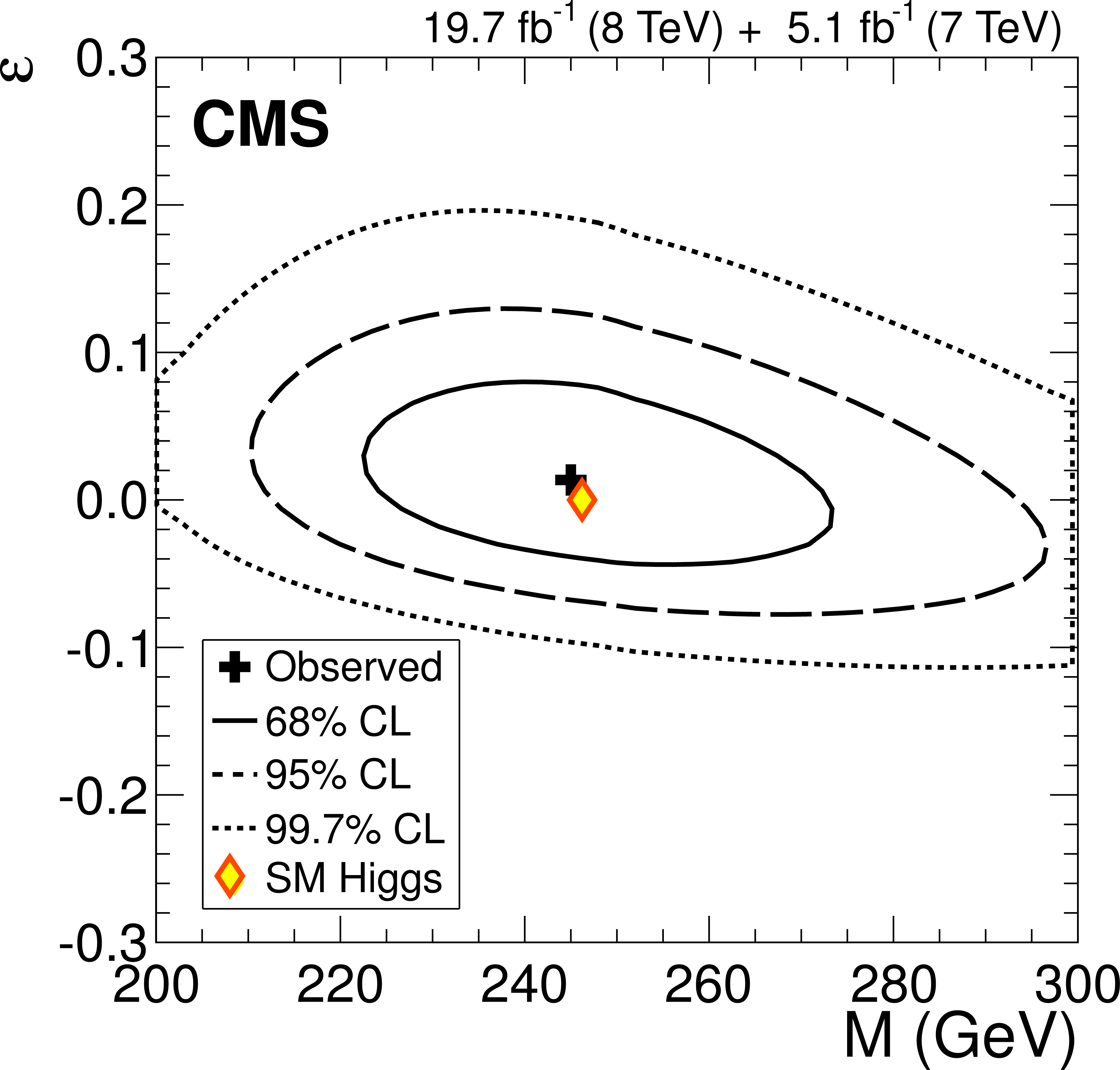
Figure 12-b:
(a) Results of likelihood scans for a model where the gluon and photon loop-induced interactions with the Higgs boson are resolved in terms of the couplings of other SM particles. The inner bars represent the 68% CL confidence intervals while the outer bars represent the 95% CL confidence intervals. When performing the scan for one parameter, the other parameters in the model are profiled. (b) The 2D likelihood scan for the $M$ and $\epsilon $ parameters of the model detailed in the text. The cross indicates the best-fit values. The solid, dashed, and dotted contours show the 68%, 95%, and 99.7% CL confidence regions, respectively. The diamond represents the SM expectation, $(M, \epsilon )=(v,0)$, where $v$ is the SM Higgs vacuum expectation value, $v $= 246.22 GeV. |
png pdf |
Figure 13:
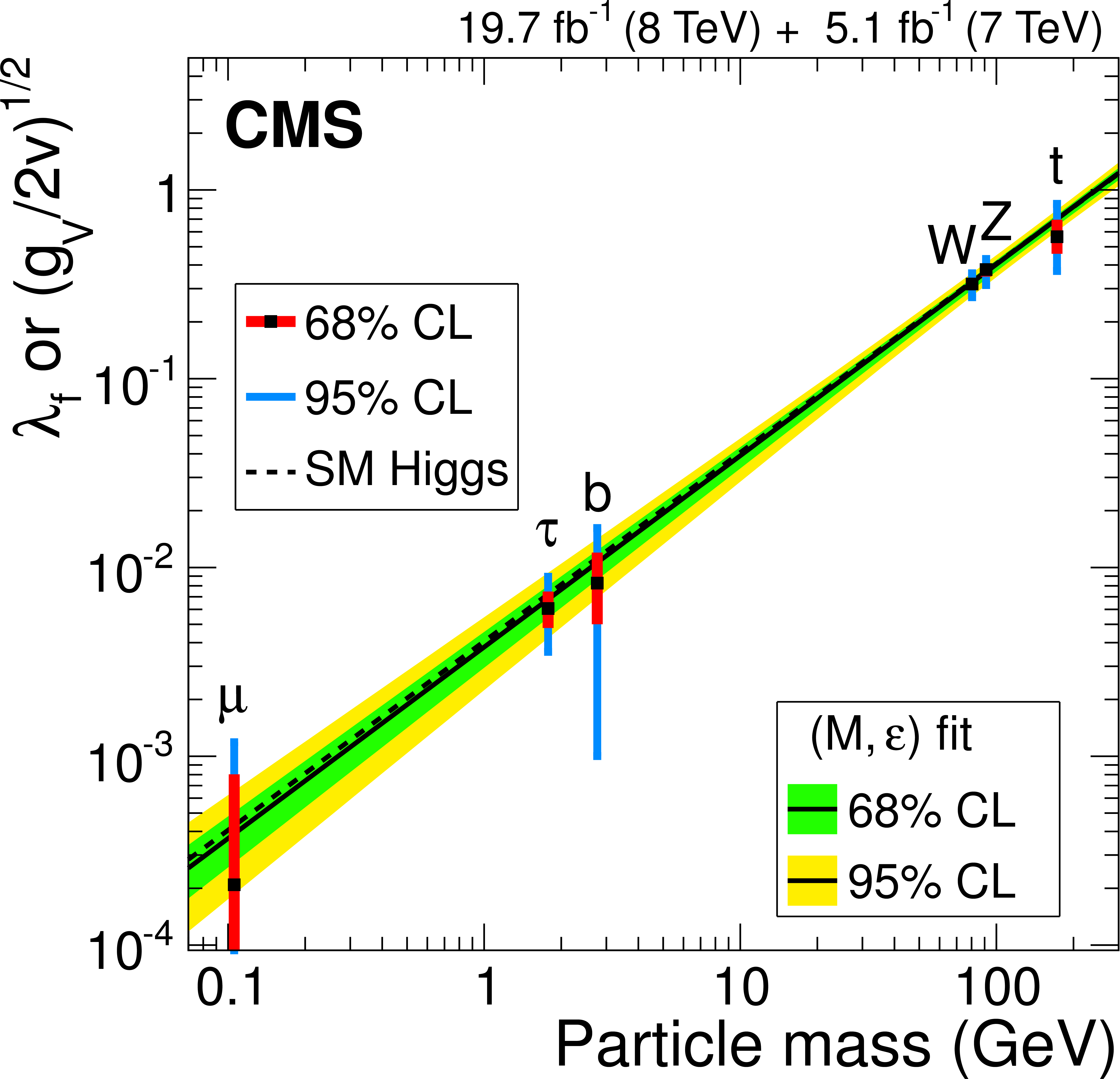
Graphical representation of the results obtained for the models considered in Fig.12. The dashed line corresponds to the SM expectation. The points from the fit in Fig.12-a are placed at particle mass values chosen as explained in the text. The ordinates are different for fermions and massive vector bosons to take into account the expected SM scaling of the coupling with mass, depending on the type of particle. The result of the $(M,\epsilon )$ fit from Fig.12-b is shown as the continuous line while the inner and outer bands represent the 68% and 95% CL confidence regions. |
png pdf |
Figure 14:
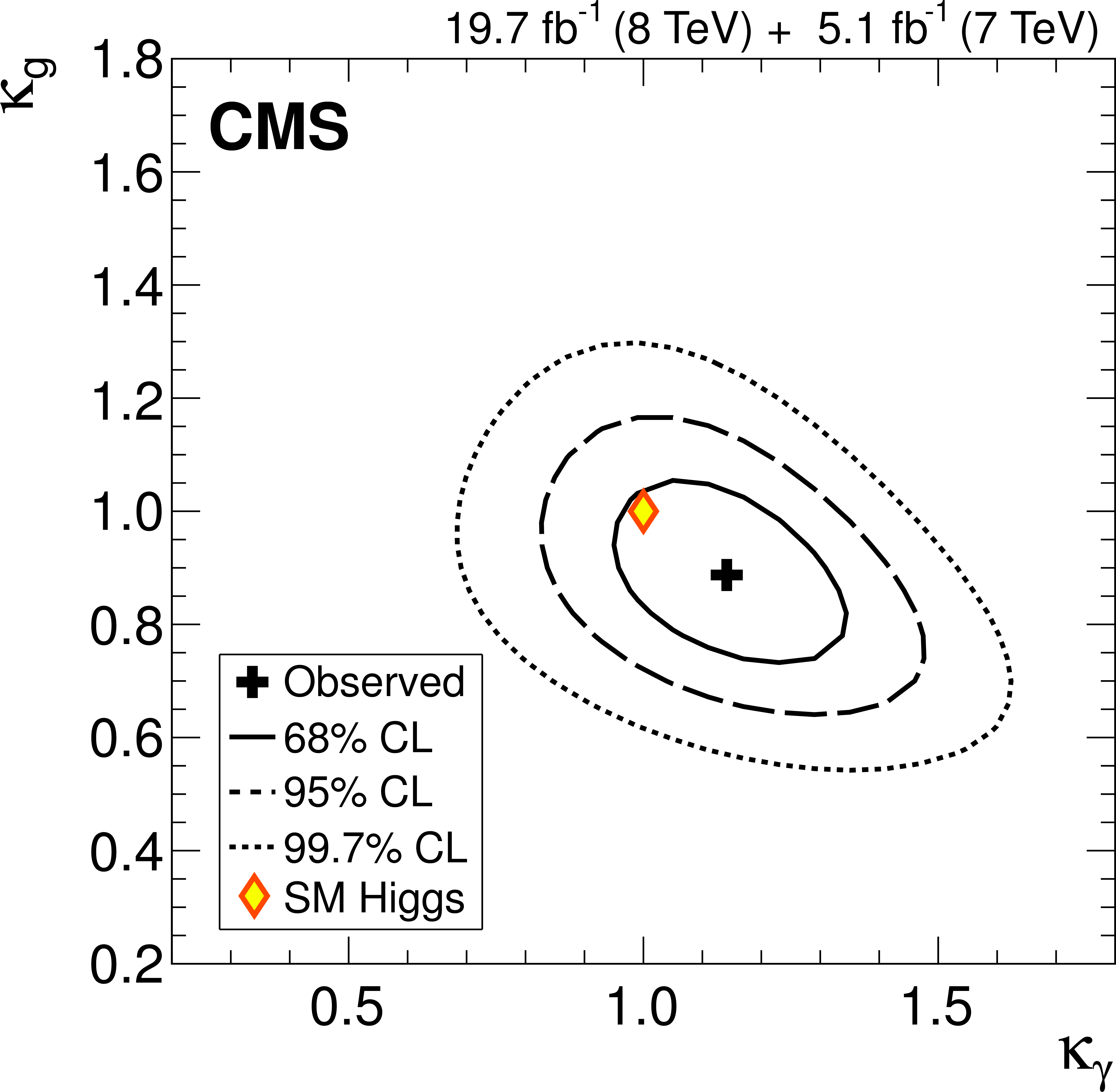
The 2D likelihood scan for the $ {\kappa _{\mathrm { {\mathrm {g}} }}} $ and $ {\kappa _{ {\gamma } }} $ parameters, assuming that $\Gamma _{\mathrm {BSM}}=0$. The cross indicates the best-fit values. The solid, dashed, and dotted contours show the 68%, 95%, and 99.7% CL confidence regions, respectively. The diamond represents the SM expectation, $( {\kappa _{ {\gamma } }} , {\kappa _{\mathrm { {\mathrm {g}} }}} )=(1,1)$. The partial widths associated with the tree-level production processes and decay modes are assumed to be unaltered ($\kappa = 1$). |
png pdf |
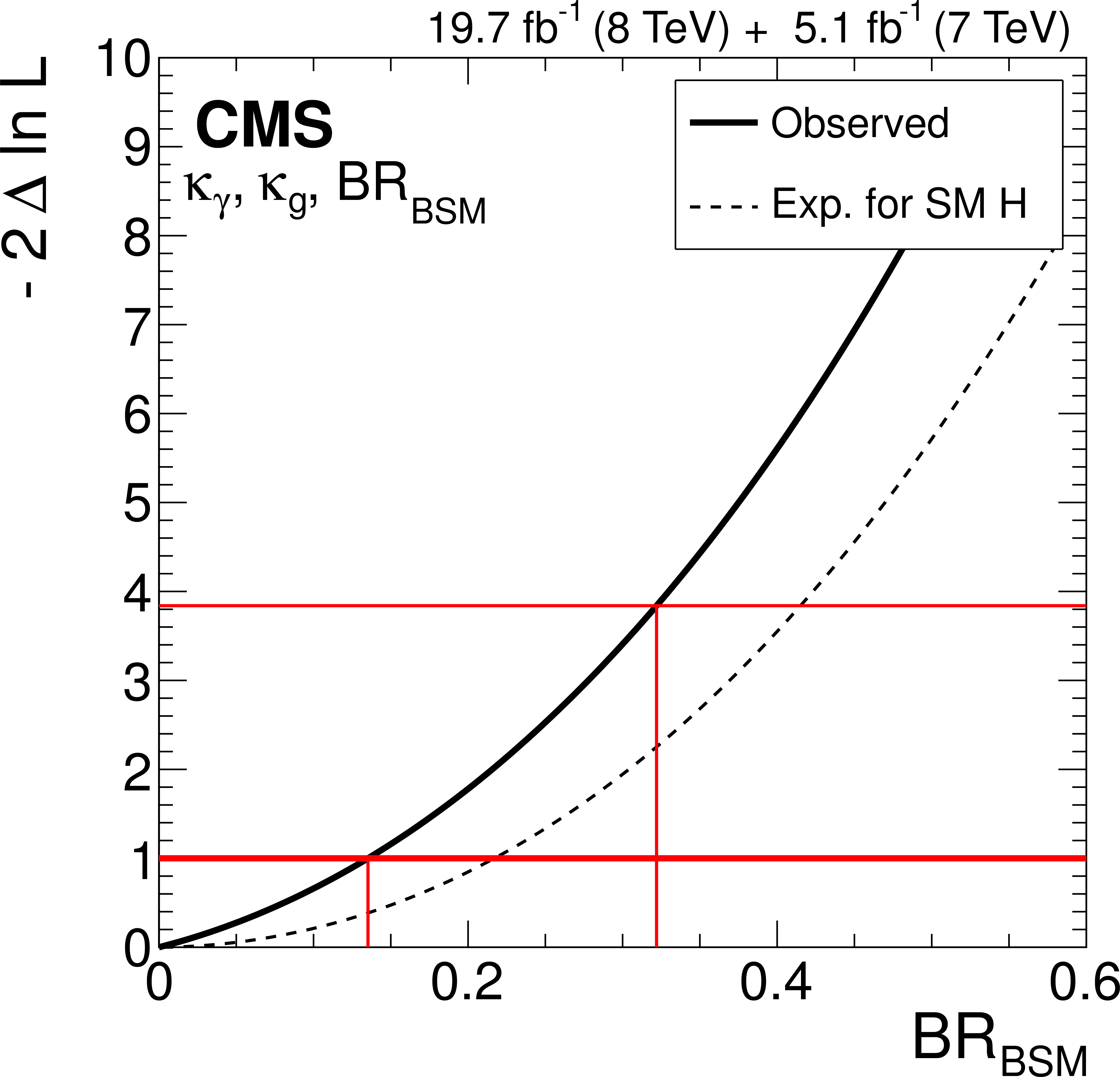
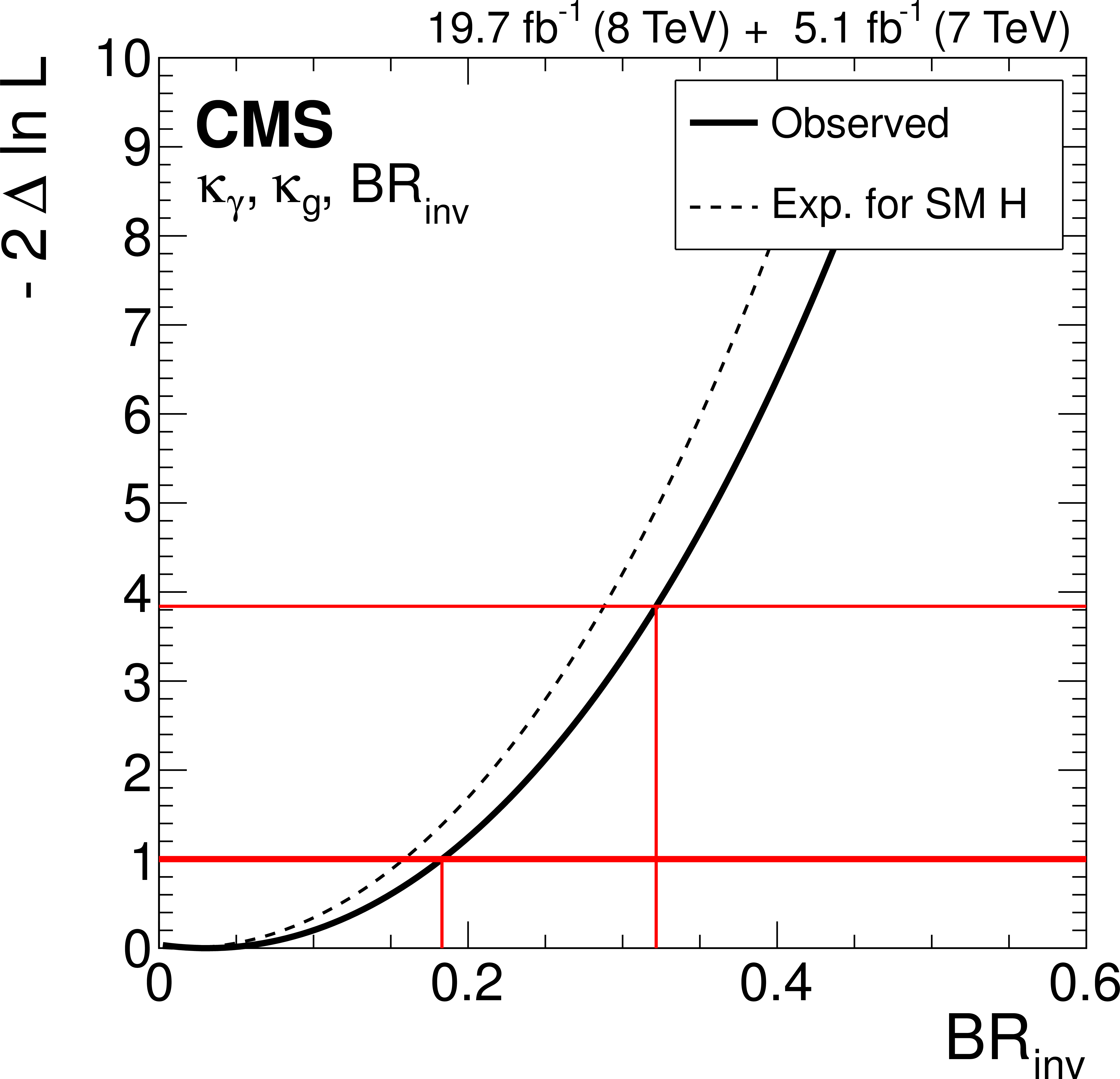
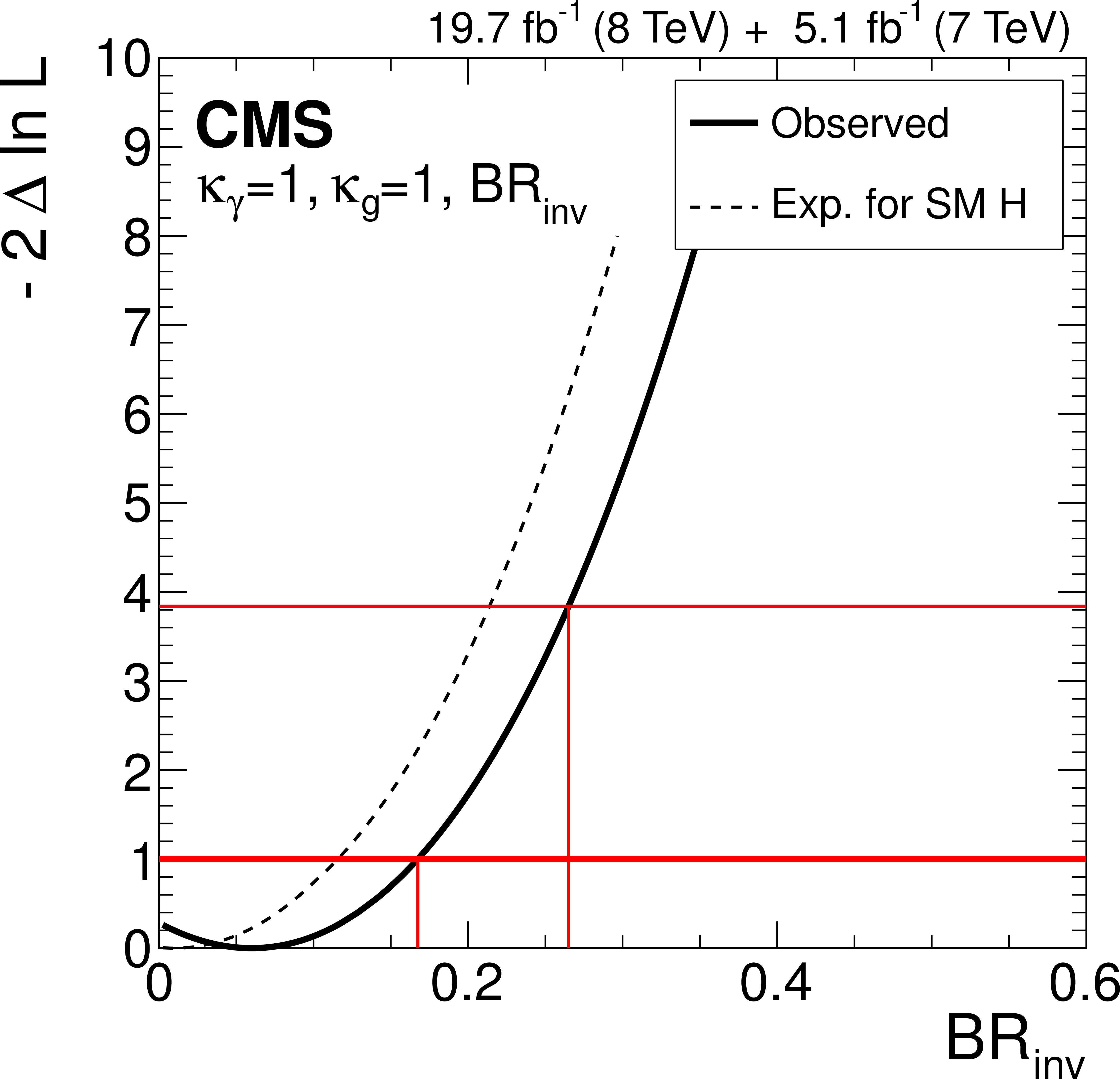
Figure 15-a:
(a) The likelihood scan versus $ {\mathrm {BR_{BSM}}} =\Gamma _{\mathrm {BSM}}/\Gamma _{\text {tot}}$. The solid curve represents the observation and the dashed curve indicates the expected median result in the presence of the SM Higgs boson. The partial widths associated with the tree-level production processes and decay modes are assumed to be as expected in the SM. (b) Result when also combining with data from the $ { {\mathrm {H}} (\mathrm {inv})} $ searches, thus assuming that $ {\mathrm {BR_{BSM}}} = {\mathrm {BR_{inv}}} $, i.e. that there are no undetected decays, $ {\mathrm {BR}_\text {undet}} $ = 0. (c) Result when further assuming that $ {\kappa _{\mathrm { {\mathrm {g}} }}} = {\kappa _{ {\gamma } }} $ = 1 and combining with the data from the $ { {\mathrm {H}} (\mathrm {inv})} $ searches. |
png pdf |
Figure 15-b:
(a) The likelihood scan versus $ {\mathrm {BR_{BSM}}} =\Gamma _{\mathrm {BSM}}/\Gamma _{\text {tot}}$. The solid curve represents the observation and the dashed curve indicates the expected median result in the presence of the SM Higgs boson. The partial widths associated with the tree-level production processes and decay modes are assumed to be as expected in the SM. (b) Result when also combining with data from the $ { {\mathrm {H}} (\mathrm {inv})} $ searches, thus assuming that $ {\mathrm {BR_{BSM}}} = {\mathrm {BR_{inv}}} $, i.e. that there are no undetected decays, $ {\mathrm {BR}_\text {undet}} $ = 0. (c) Result when further assuming that $ {\kappa _{\mathrm { {\mathrm {g}} }}} = {\kappa _{ {\gamma } }} $ = 1 and combining with the data from the $ { {\mathrm {H}} (\mathrm {inv})} $ searches. |
png pdf |
Figure 15-c:
(a) The likelihood scan versus $ {\mathrm {BR_{BSM}}} =\Gamma _{\mathrm {BSM}}/\Gamma _{\text {tot}}$. The solid curve represents the observation and the dashed curve indicates the expected median result in the presence of the SM Higgs boson. The partial widths associated with the tree-level production processes and decay modes are assumed to be as expected in the SM. (b) Result when also combining with data from the $ { {\mathrm {H}} (\mathrm {inv})} $ searches, thus assuming that $ {\mathrm {BR_{BSM}}} = {\mathrm {BR_{inv}}} $, i.e. that there are no undetected decays, $ {\mathrm {BR}_\text {undet}} $ = 0. (c) Result when further assuming that $ {\kappa _{\mathrm { {\mathrm {g}} }}} = {\kappa _{ {\gamma } }} $ = 1 and combining with the data from the $ { {\mathrm {H}} (\mathrm {inv})} $ searches. |
png pdf |
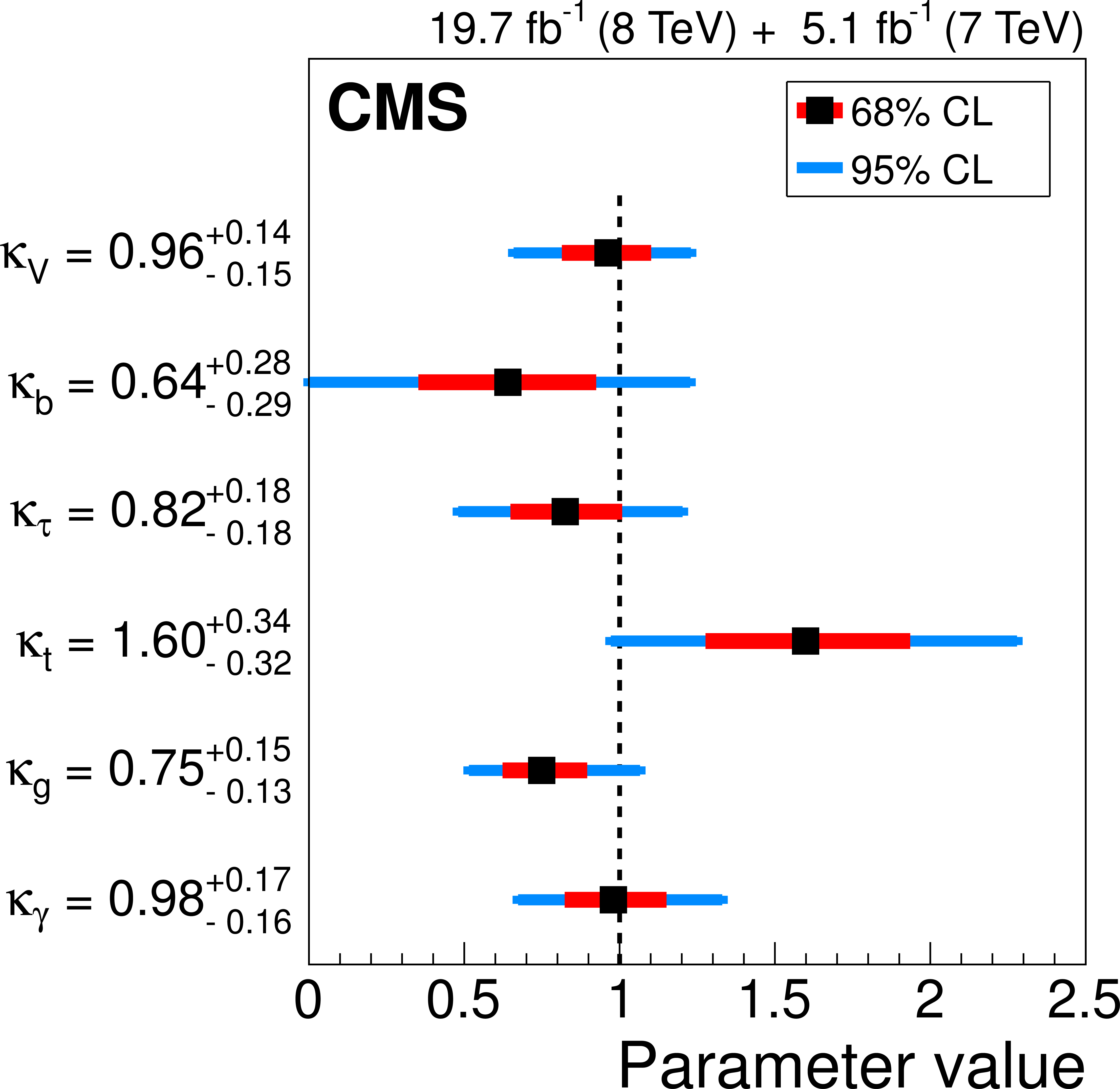
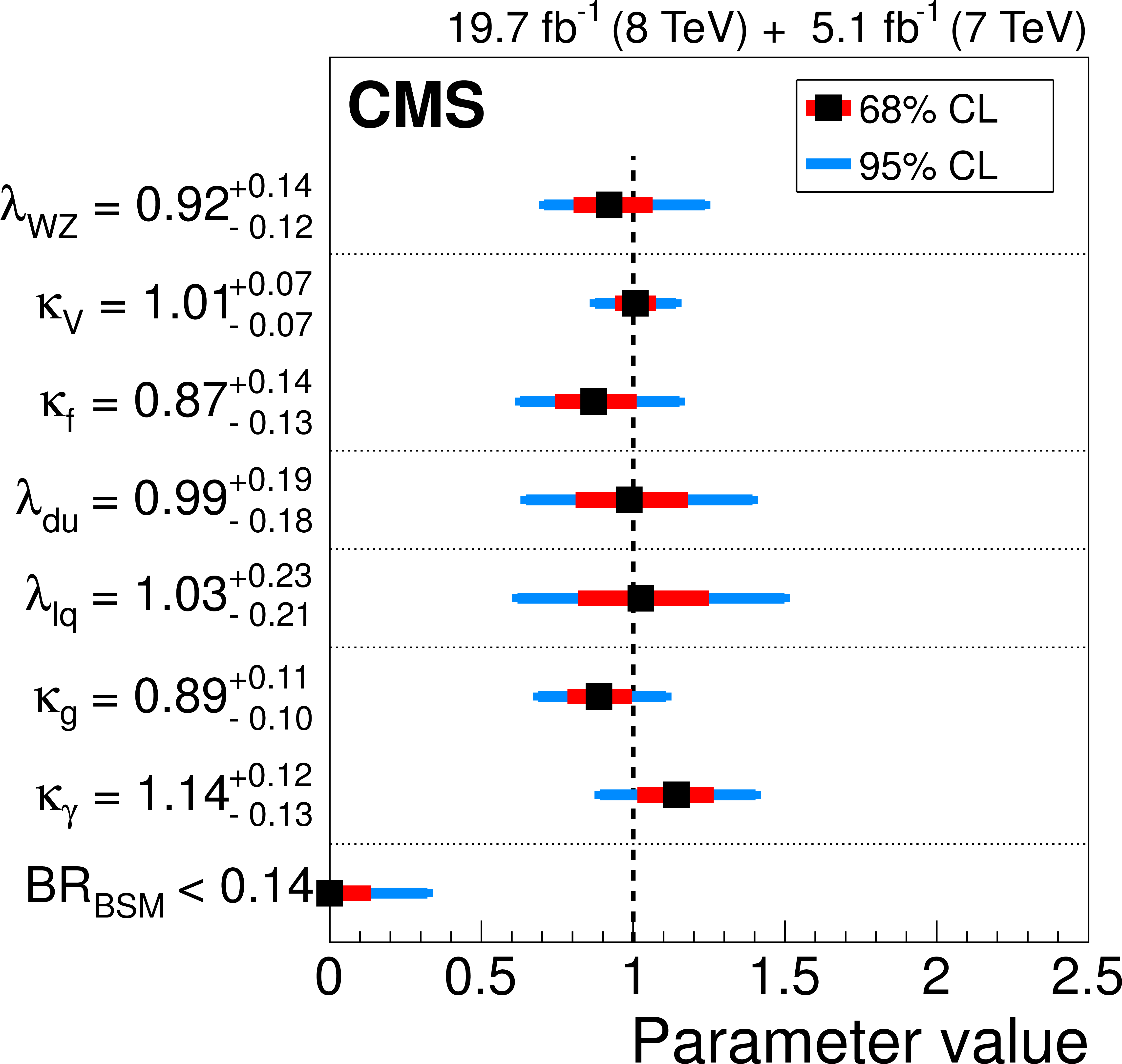
Figure 16:
Likelihood scans for parameters in a model with coupling scaling factors for the SM particles, one coupling at a time while profiling the remaining five together with all other nuisance parameters; from top to bottom: $ {\kappa _{\mathrm {V}}} $ (W and Z bosons), $ {\kappa _{ {\mathrm {b}}}} $ (bottom quarks), $ {\kappa _{ {\tau } }} $ (tau leptons), $ {\kappa _{ {\mathrm {t}}}} $ (top quarks), $ {\kappa _{\mathrm { {\mathrm {g}} }}} $ (gluons; effective coupling), and $ {\kappa _{ {\gamma } }} $ (photons; effective coupling). The inner bars represent the 68% CL confidence intervals while the outer bars represent the 95% CL confidence intervals. |
png pdf |
Figure 17:
Likelihood scans for parameters in a model without assumptions on the total width and with six coupling modifier ratios, one parameter at a time while profiling the remaining six together with all other nuisance parameters; from top to bottom: $ {\kappa _{ {\mathrm {g}} {\mathrm {Z}}}} $ ($= {\kappa _{\mathrm { {\mathrm {g}} }}} {\kappa _{\mathrm { {\mathrm {Z}}}}} / {\kappa _{ {\mathrm {H}} }} $), $ {\lambda _{\mathrm { {\mathrm {W}} {\mathrm {Z}}}}} $ ($= {\kappa _{\mathrm { {\mathrm {W}}}}} / {\kappa _{\mathrm { {\mathrm {Z}}}}} $), $ {\lambda _{ {\mathrm {Z}} {\mathrm {g}} }} $ ($= {\kappa _{\mathrm { {\mathrm {Z}}}}} / {\kappa _{\mathrm { {\mathrm {g}} }}} $), $ {\lambda _{ {\mathrm {b}} {\mathrm {Z}}}} $ ($= {\kappa _{ {\mathrm {b}}}} / {\kappa _{\mathrm { {\mathrm {Z}}}}} $), $ {\lambda _{ {\gamma } {\mathrm {Z}}}} $ ($= {\kappa _{ {\gamma } }} / {\kappa _{\mathrm { {\mathrm {Z}}}}} $), $ {\lambda _{ {\tau } {\mathrm {Z}}}} $ ($= {\kappa _{ {\tau } }} / {\kappa _{\mathrm { {\mathrm {Z}}}}} $), and $ {\lambda _{ {\mathrm {t}} {\mathrm {g}}}} $ ($= {\kappa _{ {\mathrm {t}}}} / {\kappa _{\mathrm { {\mathrm {g}} }}} $). The inner bars represent the 68% CL confidence intervals while the outer bars represent the 95% CL confidence intervals. |
png pdf |
Figure 18-a:
(a) Likelihood scan versus $ {\mathrm {BR_{BSM}}} =\Gamma _{\mathrm {BSM}}/\Gamma _{\text {tot}}$. The solid curve represents the observation in data and the dashed curve indicates the expected median result in the presence of the SM Higgs boson. The modifiers for both the tree-level and loop-induced couplings are profiled, but the couplings to the electroweak bosons are assumed to be bounded by the SM expectation ($ {\kappa _{\mathrm {V}}} \le 1$). (b) Result when also combining with data from the $ { {\mathrm {H}} (\mathrm {inv})} $ searches, thus assuming that $ {\mathrm {BR_{BSM}}} = {\mathrm {BR_{inv}}} $, i.e. $ {\mathrm {BR}_\text {undet}} =0$. |
png pdf |
Figure 18-b:
(a) Likelihood scan versus $ {\mathrm {BR_{BSM}}} =\Gamma _{\mathrm {BSM}}/\Gamma _{\text {tot}}$. The solid curve represents the observation in data and the dashed curve indicates the expected median result in the presence of the SM Higgs boson. The modifiers for both the tree-level and loop-induced couplings are profiled, but the couplings to the electroweak bosons are assumed to be bounded by the SM expectation ($ {\kappa _{\mathrm {V}}} \le 1$). (b) Result when also combining with data from the $ { {\mathrm {H}} (\mathrm {inv})} $ searches, thus assuming that $ {\mathrm {BR_{BSM}}} = {\mathrm {BR_{inv}}} $, i.e. $ {\mathrm {BR}_\text {undet}} =0$. |
png pdf |
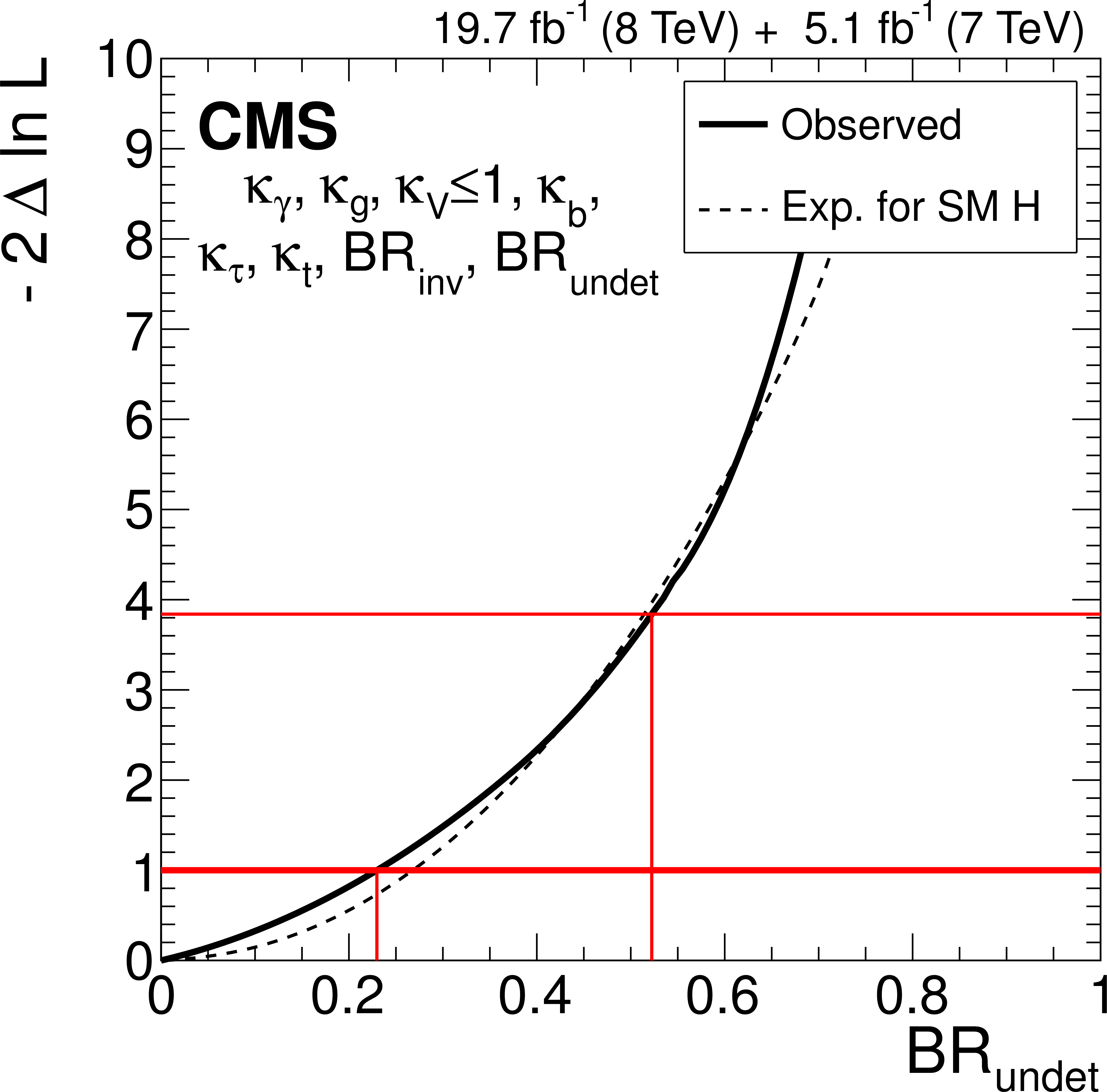
Figure 19-a:
(a) The 2D likelihood scan for the $ {\mathrm {BR_{inv}}} $ and $ {\mathrm {BR}_\text {undet}} $ parameters for a combined analysis of the $ { {\mathrm {H}} (\mathrm {inv})} $ search data and visible decay channels. The cross indicates the best-fit values. The solid, dashed, and dotted contours show the 68%, 95%, and 99.7% CL confidence regions, respectively. The diamond represents the SM expectation, $( {\mathrm {BR_{inv}}} , {\mathrm {BR}_\text {undet}} )=(0,0)$. (b) The likelihood scan versus $ {\mathrm {BR}_\text {undet}} $. The solid curve represents the observation in data and the dashed curve indicates the expected median result in the presence of the SM Higgs boson. $ {\mathrm {BR_{inv}}} $ is constrained by the data from the $ { {\mathrm {H}} (\mathrm {inv})} $ searches and modifiers for both the tree-level and loop-induced couplings are profiled, but the couplings to the electroweak bosons are assumed to be bounded by the SM expectation ($ {\kappa _{\mathrm {V}}} \le 1$). |
png pdf |
Figure 19-b:
(a) The 2D likelihood scan for the $ {\mathrm {BR_{inv}}} $ and $ {\mathrm {BR}_\text {undet}} $ parameters for a combined analysis of the $ { {\mathrm {H}} (\mathrm {inv})} $ search data and visible decay channels. The cross indicates the best-fit values. The solid, dashed, and dotted contours show the 68%, 95%, and 99.7% CL confidence regions, respectively. The diamond represents the SM expectation, $( {\mathrm {BR_{inv}}} , {\mathrm {BR}_\text {undet}} )=(0,0)$. (b) The likelihood scan versus $ {\mathrm {BR}_\text {undet}} $. The solid curve represents the observation in data and the dashed curve indicates the expected median result in the presence of the SM Higgs boson. $ {\mathrm {BR_{inv}}} $ is constrained by the data from the $ { {\mathrm {H}} (\mathrm {inv})} $ searches and modifiers for both the tree-level and loop-induced couplings are profiled, but the couplings to the electroweak bosons are assumed to be bounded by the SM expectation ($ {\kappa _{\mathrm {V}}} \le 1$). |
png pdf |
Figure 20:
Summary plot of likelihood scan results for the different parameters of interest in benchmark models from Ref. separated by dotted lines. The $ {\mathrm {BR_{BSM}}} $ value at the bottom is obtained for the model with three parameters $( {\kappa _{\mathrm { {\mathrm {g}} }}} , {\kappa _{ {\gamma } }} , {\mathrm {BR_{BSM}}} )$. The inner bars represent the 68% CL confidence intervals while the outer bars represent the 95% CL confidence intervals. |
| Tables | |
png pdf |
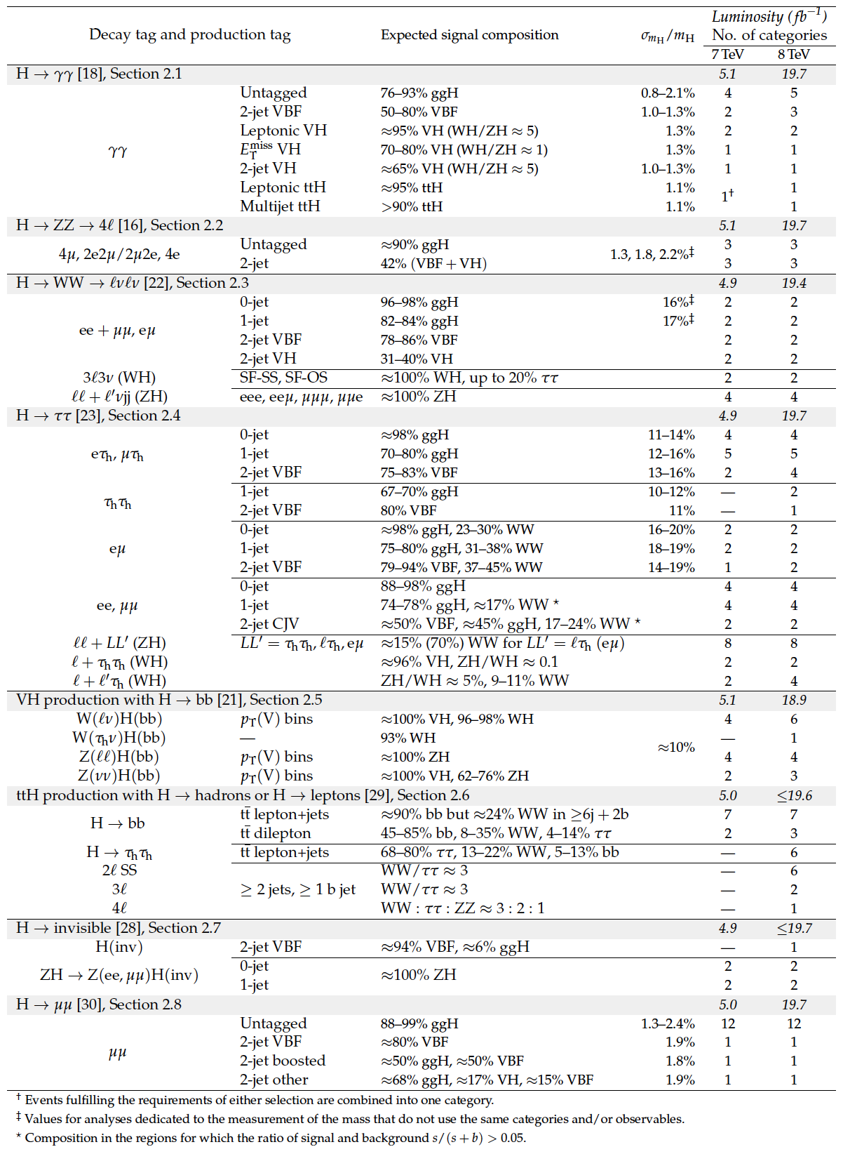
Table 1:
Summary of the channels in the analyses included in this combination. The first and second columns indicate which decay mode and production mechanism is targeted by an analysis. Notes on the expected composition of the signal are given in the third column. Where available, the fourth column specifies the expected relative mass resolution for the SM Higgs boson. Finally, the last columns provide the number of event categories and the integrated luminosity for the 7 and 8 TeV data sets. The notation is explained in the text. |
png pdf |
Table 2:
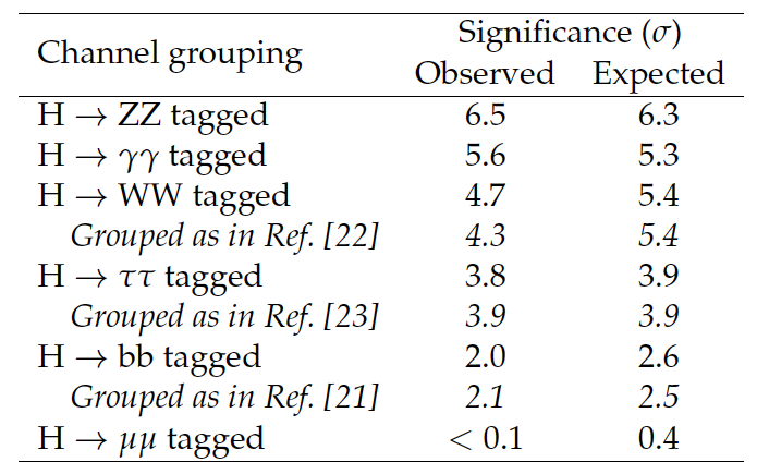
The observed and median expected significances of the excesses for each decay mode group, assuming $ {m_\mathrm { {\mathrm {H}} }} = $ 125.0 GeV. The channels are grouped by decay mode tag as described in the text; when there is a difference in the channels included with respect to the published results for the individual channels, the result for the grouping used in those publications is also given. |
png pdf |
Table 3:
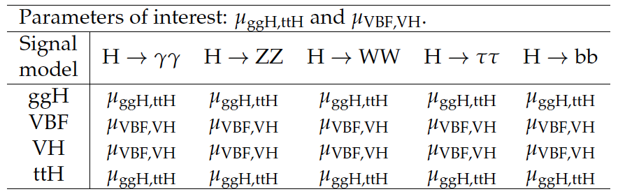
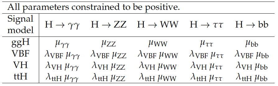
Parameterization used to scale the expected SM Higgs boson yields from the different production modes when obtaining the results presented in Table 5 and Fig.5(a). The signal strength modifiers $ {\mu _{ { {\mathrm {g}} {\mathrm {g}} {\mathrm {H}} } , { {\mathrm {t}} {\mathrm {t}} {\mathrm {H}} } }} $ and $ {\mu _{ {\mathrm {VBF}} , {\mathrm {V} {\mathrm {H}} } }} $, common to all decay modes, are associated with the $ { {\mathrm {g}} {\mathrm {g}} {\mathrm {H}} } $ and ${ {\mathrm {t}} {\mathrm {t}} {\mathrm {H}} } $ and with the $ {\mathrm {VBF}} $ and $ {\mathrm {V} {\mathrm {H}} } $ production mechanisms, respectively. |
png pdf |
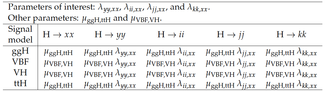
Table 4:
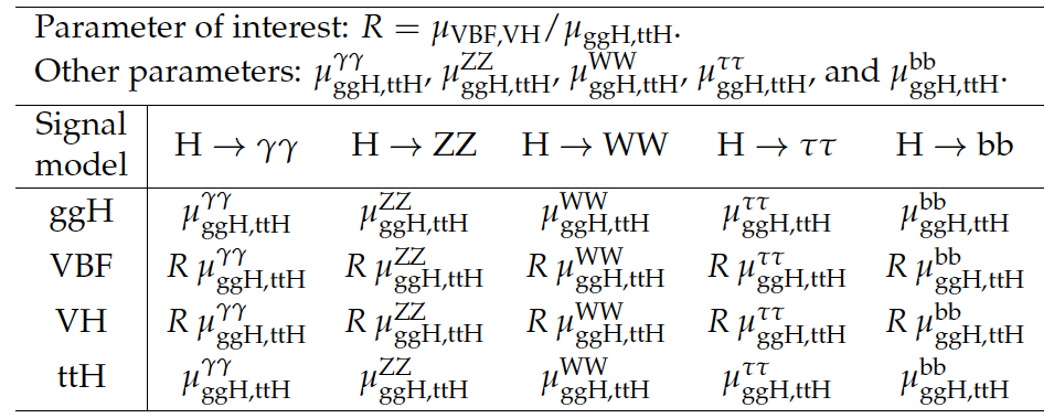
Parameterization used to scale the expected SM Higgs boson yields for the different production processes and decay modes when obtaining the $ { {\mu _{ {\mathrm {VBF}} , {\mathrm {V} {\mathrm {H}} } }} / {\mu _{ { {\mathrm {g}} {\mathrm {g}} {\mathrm {H}} } , { {\mathrm {t}} {\mathrm {t}} {\mathrm {H}} } }} } $ results presented in Table 5 and Fig.5(b). |
png pdf |
Table 5:
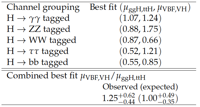
The best-fit values for the signal strength of the $ {\mathrm {VBF}} $ and $ {\mathrm {V} {\mathrm {H}} } $ and of the ${ {\mathrm {g}} {\mathrm {g}} {\mathrm {H}} } $ and $ { {\mathrm {t}} {\mathrm {t}} {\mathrm {H}} } $ production mechanisms, $ {\mu _{ {\mathrm {VBF}} , {\mathrm {V} {\mathrm {H}} } }} $ and $ {\mu _{ { {\mathrm {g}} {\mathrm {g}} {\mathrm {H}} } , { {\mathrm {t}} {\mathrm {t}} {\mathrm {H}} } }} $, respectively, for $ {m_\mathrm { {\mathrm {H}} }} = $ 125.0 GeV. The channels are grouped by decay mode tag as described in the text. The observed and median expected results for the ratio of $ {\mu _{ {\mathrm {VBF}} , {\mathrm {V} {\mathrm {H}} } }} $ to $ {\mu _{ { {\mathrm {g}} {\mathrm {g}} {\mathrm {H}} } , { {\mathrm {t}} {\mathrm {t}} {\mathrm {H}} } }} $ together with their uncertainties are also given for the full combination. In the full combination, $ { {\mu _{ {\mathrm {VBF}} , {\mathrm {V} {\mathrm {H}} } }} / {\mu _{ { {\mathrm {g}} {\mathrm {g}} {\mathrm {H}} } , { {\mathrm {t}} {\mathrm {t}} {\mathrm {H}} } }} } $ is determined while profiling the five $ {\mu _{ { {\mathrm {g}} {\mathrm {g}} {\mathrm {H}} } , { {\mathrm {t}} {\mathrm {t}} {\mathrm {H}} } }} $ parameters, one per decay mode, as shown in Table 4. |
png pdf |
Table 6:
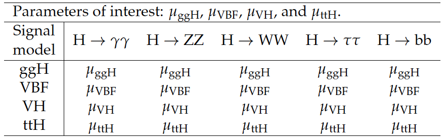
Parameterization used to scale the expected SM Higgs boson yields of the different production and decay modes when obtaining the results presented in Fig.6. |
png pdf |
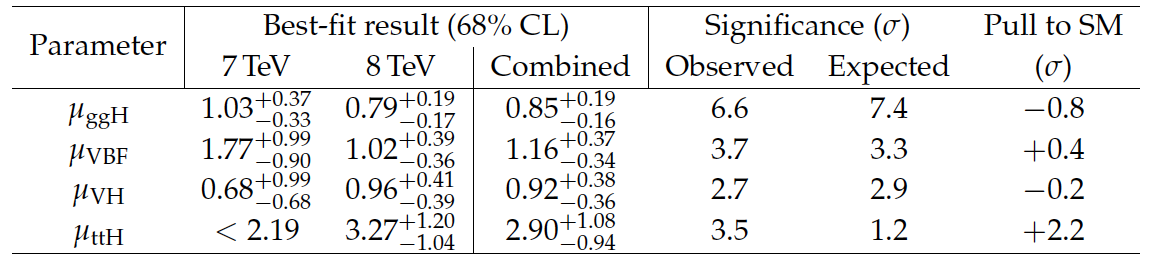
Table 7:
The best-fit results for independent signal strengths scaling the $ { {\mathrm {g}} {\mathrm {g}} {\mathrm {H}} } $, ${\mathrm {VBF}} $, $ {\mathrm {V} {\mathrm {H}} } $, and $ { {\mathrm {t}} {\mathrm {t}} {\mathrm {H}} } $ production processes; the expected and observed significances with respect to the background-only hypothesis, $\mu _{i}=0$; and the pull of the observation with respect to the SM hypothesis, $\mu _{i}=1$. The best-fit results are also provided separately for the 7 TeV and 8 TeV data sets, for which the predicted cross sections differ. These results assume that the relative values of the branching fractions are those predicted for the SM Higgs boson. |
png pdf |
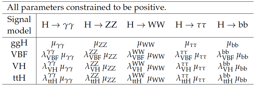
Table 8:
Parameterization used to scale the expected SM Higgs boson yields of the different production and decay modes when obtaining the results presented in Table 9. The $ {\mu _{ { {\mathrm {g}} {\mathrm {g}} {\mathrm {H}} } , { {\mathrm {t}} {\mathrm {t}} {\mathrm {H}} } }} $ and $ {\mu _{ {\mathrm {VBF}} , {\mathrm {V} {\mathrm {H}} } }} $ parameters are introduced to reduce the dependency of the results on the SM expectation. |
png pdf |
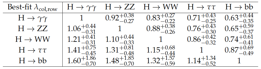
Table 9:
The best-fit results and 68\%CL confidence intervals for signal strength ratios of the decay mode in each column and the decay mode in each row, as modelled by the parameterization in Table 8. When the likelihood of the data is scanned as a function of each individual parameter, the three other parameters in the same row, as well the production cross sections modifiers $ {\mu _{ { {\mathrm {g}} {\mathrm {g}} {\mathrm {H}} } , { {\mathrm {t}} {\mathrm {t}} {\mathrm {H}} } }} $ and $ {\mu _{ {\mathrm {VBF}} , {\mathrm {V} {\mathrm {H}} } }} $, are profiled. Since each row corresponds to an independent fit to data, the relation $\lambda _{yy,xx}=1/\lambda _{xx,yy}$ is only approximately satisfied. |
png pdf |
Table 10:
A completely general signal parameterization used to scale the expected yields of the $5\times 4$ different production and decay modes. The particular choice of parameters is such that the single-particle parameterization shown in Table 11 is a nested model, i.e. it can be obtained by assuming $\lambda _{i}^{j}=\lambda _{i}$, where $i$ runs through the production processes except $ { {\mathrm {g}} {\mathrm {g}} {\mathrm {H}} } $ and $j$ runs through the decay modes. The expectation for the SM Higgs boson is $\lambda _{i}^{j}=\mu _{j}=1$. This parameterization is used in the denominator of the test statistic defined in Eq.6. |
png pdf |
Table 11:
A general single-state parameterization used to scale the expected yields of the different production and decay modes. For this parameterization the matrix has rank${( {\mathcal {M}} )} =$ 1 by definition. It can be seen that this parameterization is nested in the general one presented in Table 10, and can be obtained by setting $\lambda _{i}^{j}=\lambda _{i}$, where $i$ runs through the production processes except $ { {\mathrm {g}} {\mathrm {g}} {\mathrm {H}} } $ and $j$ runs through the decay modes. The expectation for the SM Higgs boson is $\lambda _{i}=\mu _{j}=1$. This parameterization is used in the numerator of the test statistic defined in Eq.6. |

png pdf |
Table 12:
Tests of the compatibility of the data with the SM Higgs boson couplings. The best-fit values and 68% and 95%CL confidence intervals are given for the evaluated scaling factors $\kappa _{i}$ or ratios $\lambda _{ij}=\kappa _{i}/\kappa _{j}$. The different compatibility tests discussed in the text are separated by horizontal lines. When one of the parameters in a group is evaluated, others are treated as nuisance parameters. |
| Summary |
| Properties of the Higgs boson with mass near 125 GeV are measured in proton-proton collisions with the CMS experiment at the LHC. Comprehensive sets of production and decay measurements are combined. The decay channels include $\gamma\gamma$, ZZ, WW, $\tau\tau$, bb, and $\mu\mu$ pairs. The data samples were collected in 2011 and 2012 and correspond to integrated luminosities of up to 5.1 fb$^{-1}$ at 7 TeV and up to 19.7 fb$^{-1}$ at 8 TeV. From the high-resolution $\gamma\gamma$ and ZZ channels, the mass of the Higgs boson is determined to be 125.02 $^{+0.26}_{-0.27}$ (stat) $^{+0.14}_{-0.15}$ (syst) GeV. For this mass value, the event yields obtained in the different analyses tagging specific decay channels and production mechanisms are consistent with those expected for the standard model Higgs boson. The combined best-fit signal relative to the standard model expectation is 1.00 $\pm$ 0.09 (stat) $^{+0.08}_{-0.07}$ (theo) $\pm$ 0.07 (syst) at the measured mass. The couplings of the Higgs boson are probed for deviations in magnitude from the standard model predictions in multiple ways, including searches for invisible and undetected decays. No significant deviations are found. |
|
|
Compact Muon Solenoid LHC, CERN |
|

|

|

|

|

|