

Compact Muon Solenoid
LHC, CERN
| CMS-HIG-14-019 ; CERN-PH-EP-2015-264 | ||
| Search for a very light NMSSM Higgs boson produced in decays of the 125 GeV scalar boson and decaying into $\tau$ leptons in pp collisions at $\sqrt{s} =$ 8 TeV | ||
| CMS Collaboration | ||
| 22 October 2015 | ||
| J. High Energy Phys. 01 (2016) 079 | ||
| Abstract: A search for a very light Higgs boson decaying into a pair of $\tau$ leptons is presented within the framework of the next-to-minimal supersymmetric standard model. This search is based on a data set corresponding to an integrated luminosity of 19.7 fb$^{-1}$ of proton-proton collisions collected by the CMS experiment at a centre-of-mass energy of 8 TeV. The signal is defined by the production of either of the two lightest scalars, $\mathrm{ h_1 }$ or $\mathrm{ h_2 }$, via gluon-gluon fusion and subsequent decay into a pair of the lightest Higgs bosons, $\mathrm{ a_1 }$ or $\mathrm{ h_1 }$. The $\mathrm{ h_1 }$ or $\mathrm{ h_2 }$ boson is identified with the observed state at a mass of 125 GeV. The analysis searches for decays of the $\mathrm{ a_1 }\ (\mathrm{ h_1 })$ states into pairs of $\tau$ leptons and covers a mass range for the $\mathrm{ a_1 }\ (\mathrm{ h_1 })$ boson of 4 to 8 GeV. The search reveals no significant excess in data above standard model background expectations, and an upper limit is set on the signal production cross section times branching fraction as a function of the $\mathrm{ a_1 }\ (\mathrm{ h_1 })$ boson mass. The 95% confidence level limit ranges from 4.5 pb at $m_{\mathrm{ a_1 }}\ (m_{\mathrm{ h_1 }})=$ 8 GeV to 10.3 pb at $m_{\mathrm{ a_1 }}\ (m_{\mathrm{ h_1 }}) = $ 5 GeV. | ||
| Links: e-print arXiv:1510.06534 [hep-ex] (PDF) ; CDS record ; inSPIRE record ; CADI line (restricted) ; | ||
| Figures | |
png pdf |
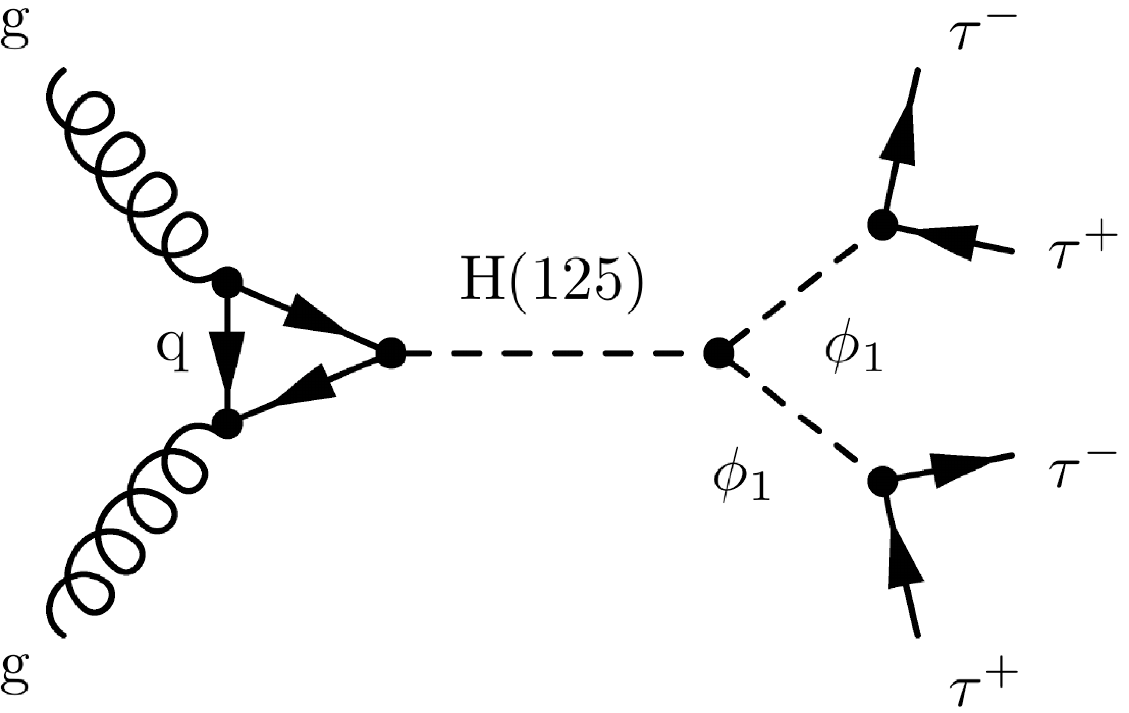
Figure 1-a:
a: Feynman diagram for the signal process. b: Illustration of the signal topology. The label ``$ {{\mu }}^\mp /\mathrm {e}^\mp /h^\mp $'' denotes a muon, electron, or charged-hadron track. |
png pdf |
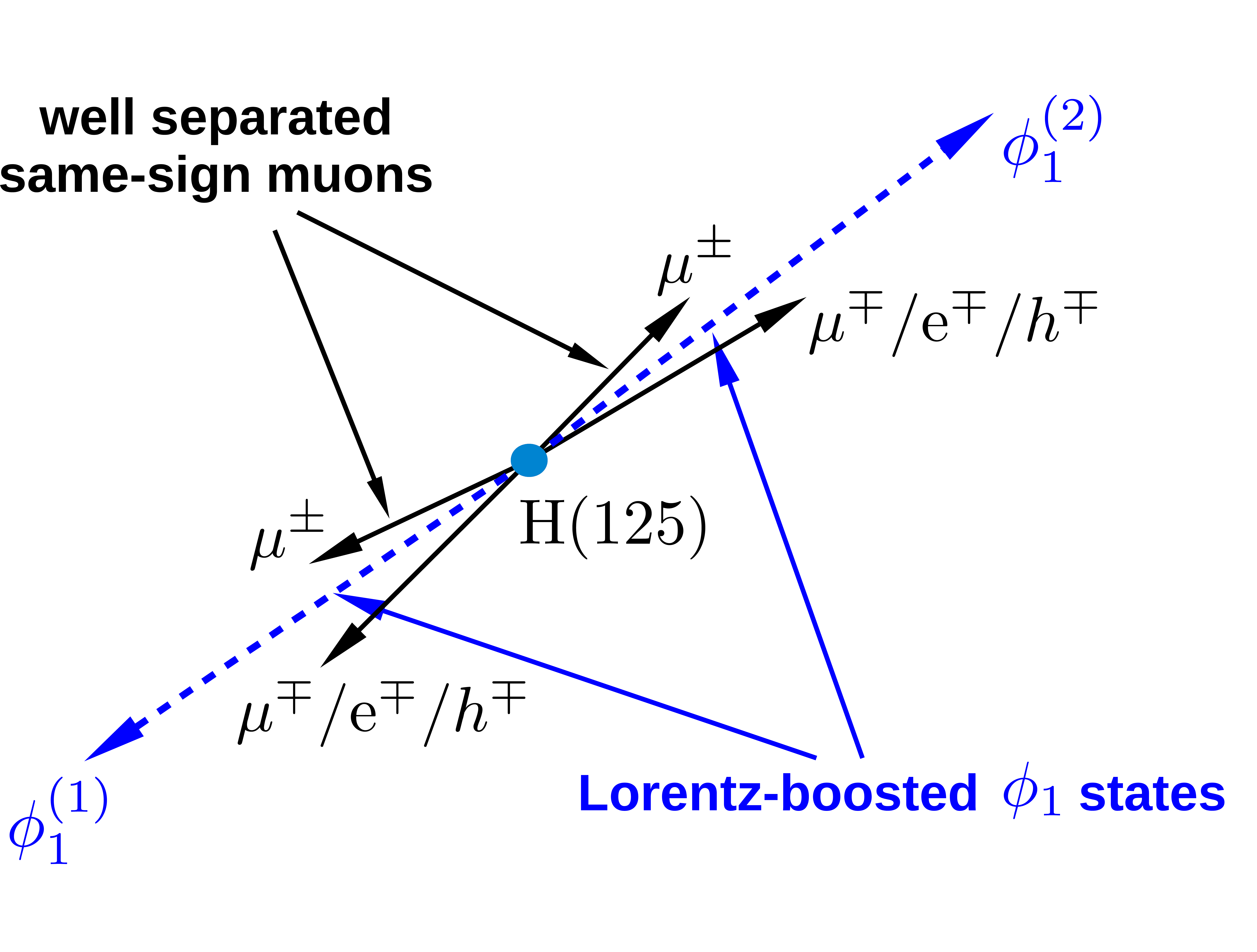
Figure 1-b:
a: Feynman diagram for the signal process. b: Illustration of the signal topology. The label ``$ {{\mu }}^\mp /\mathrm {e}^\mp /h^\mp $'' denotes a muon, electron, or charged-hadron track. |
png pdf |
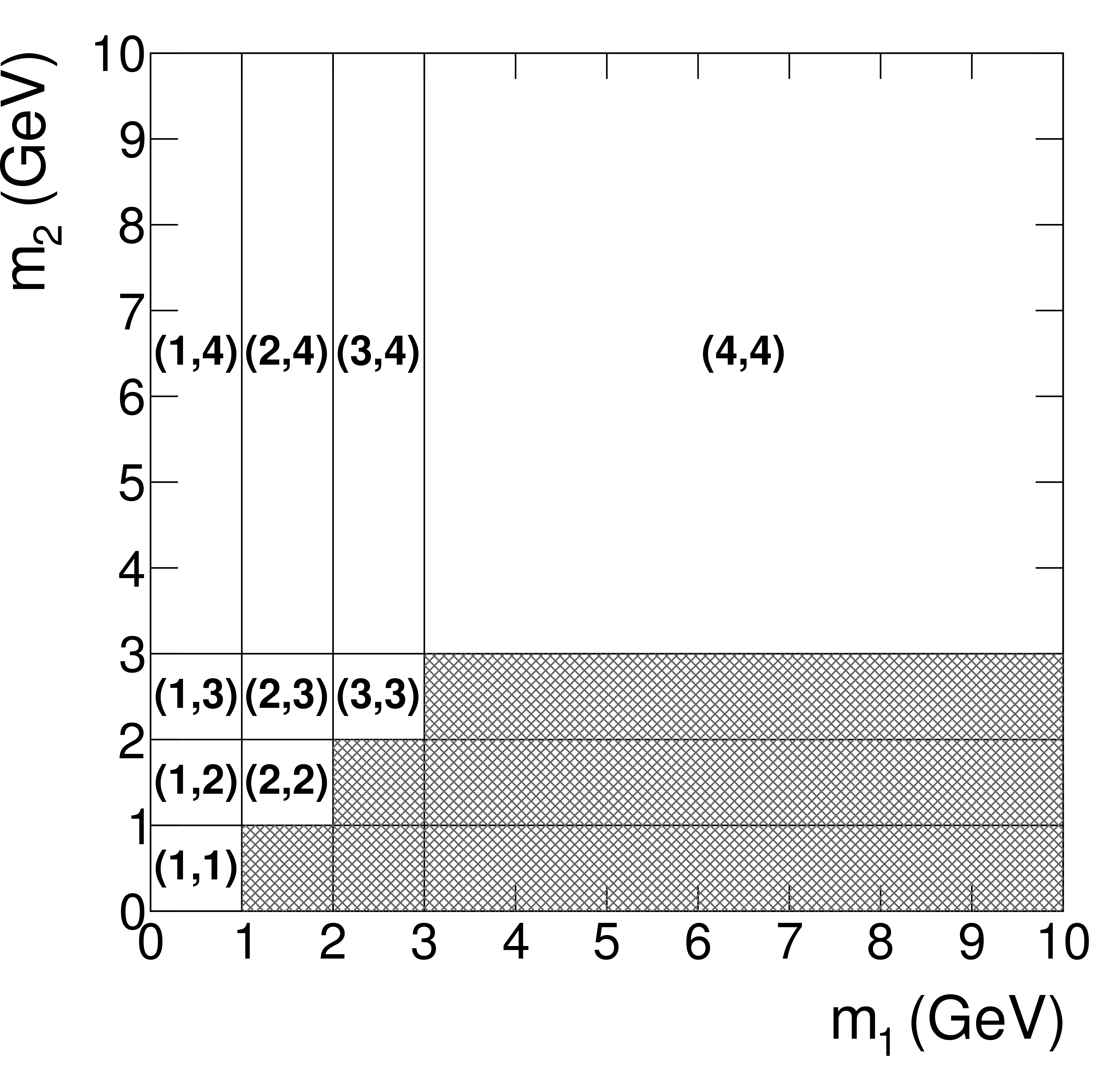
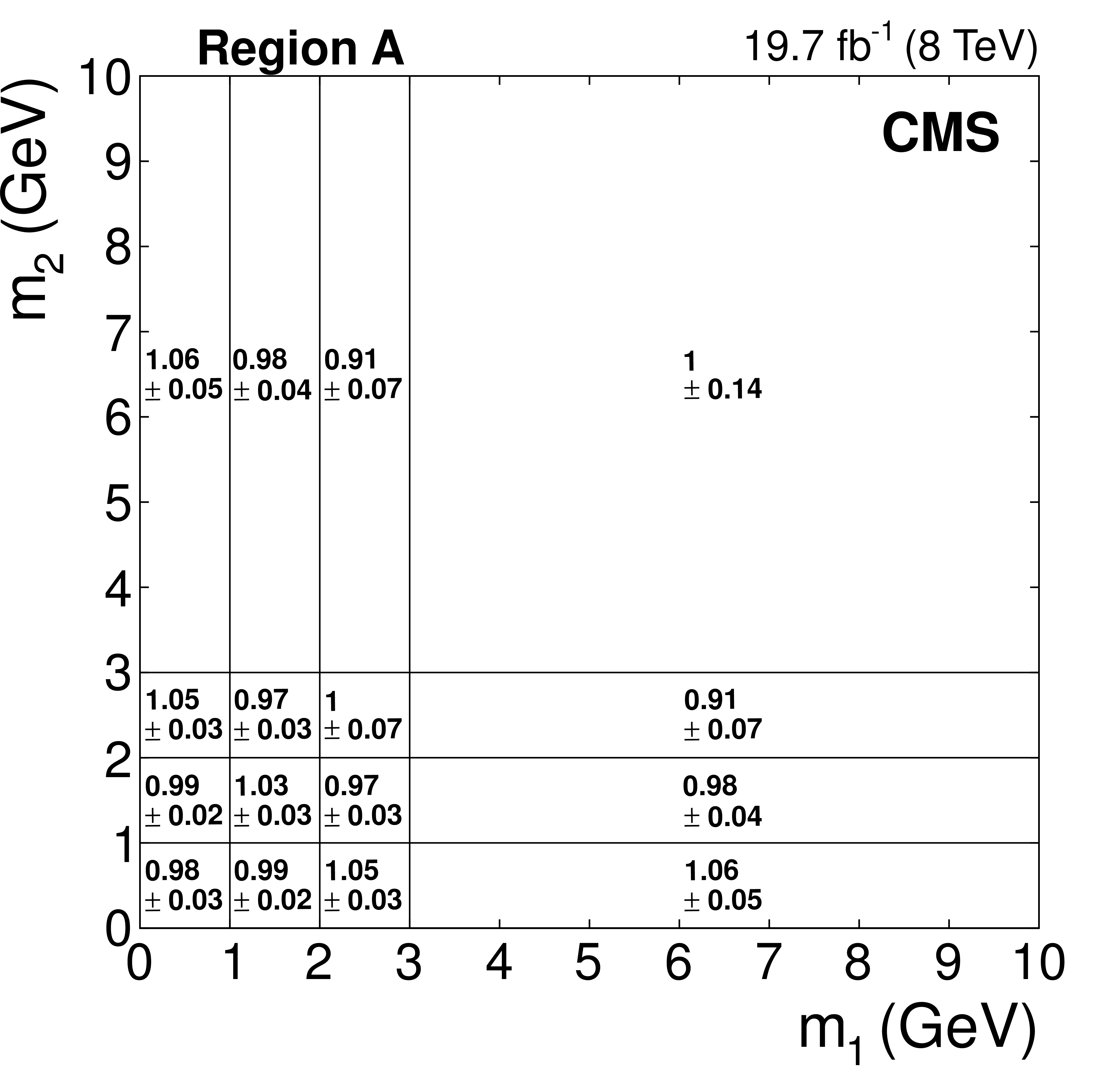
Figure 2:
Binning of the two-dimensional ($m_1,m_2$) distribution. The hatched bins are excluded from the statistical analysis, as detailed in the text. |
png pdf |
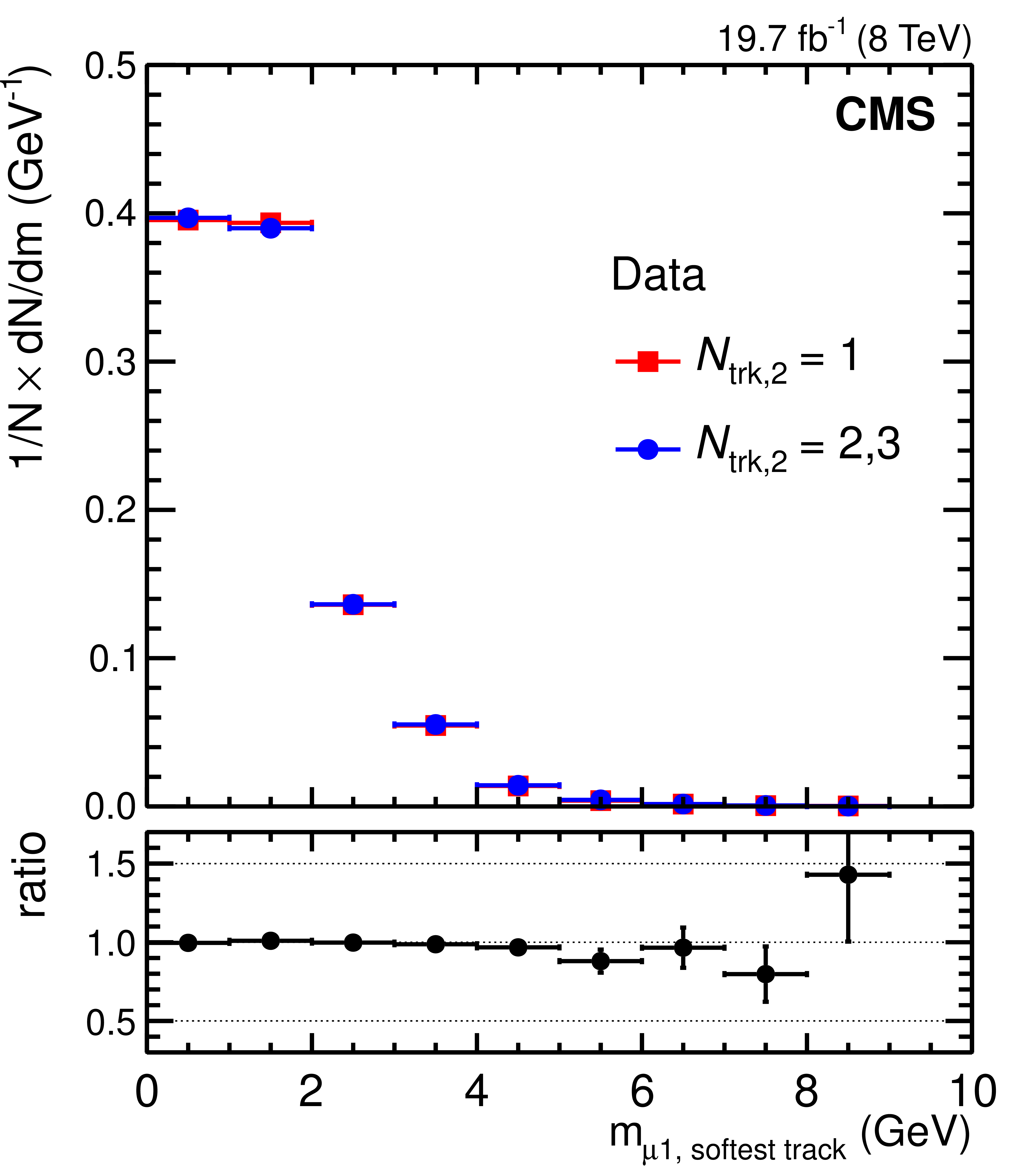
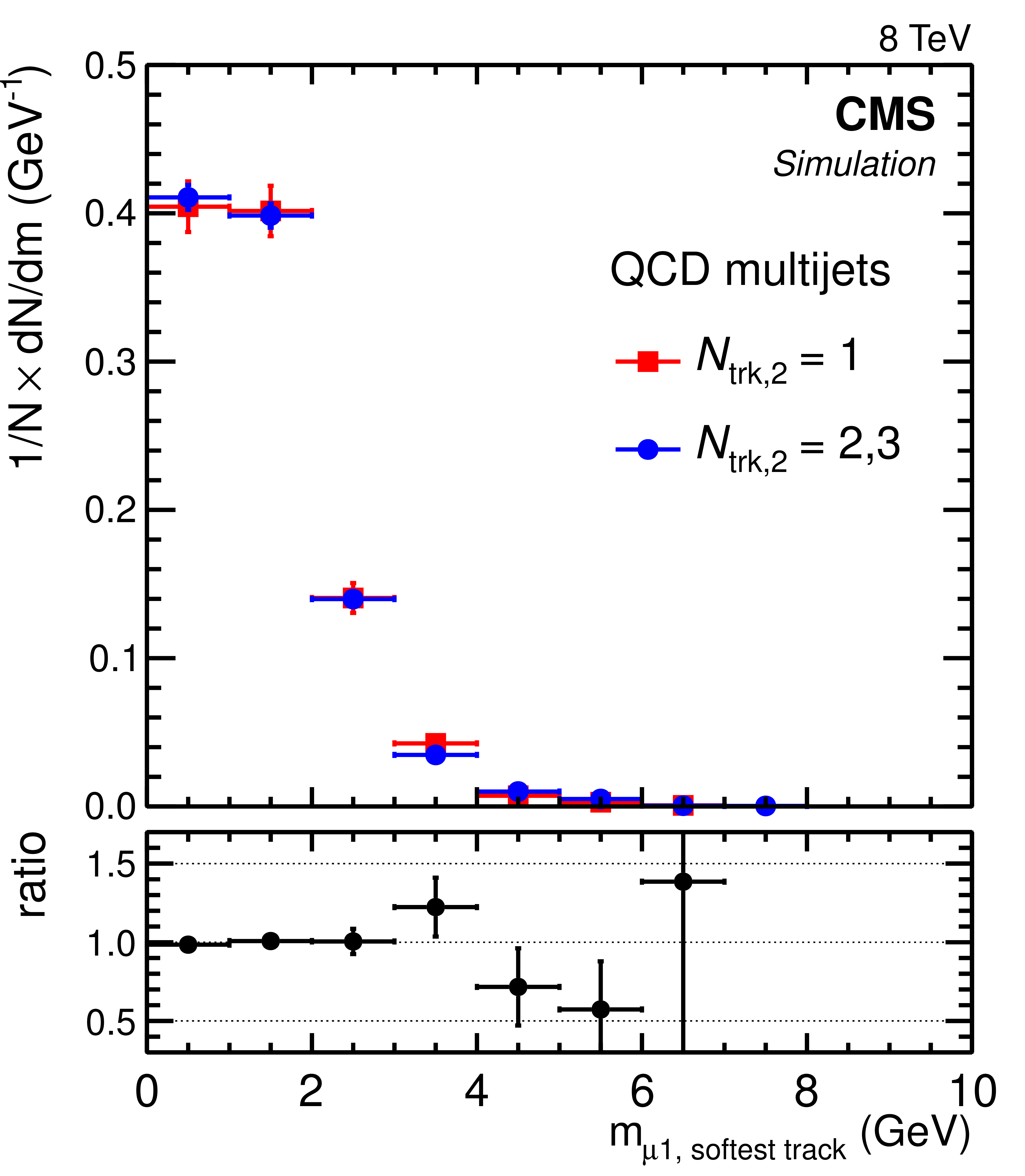
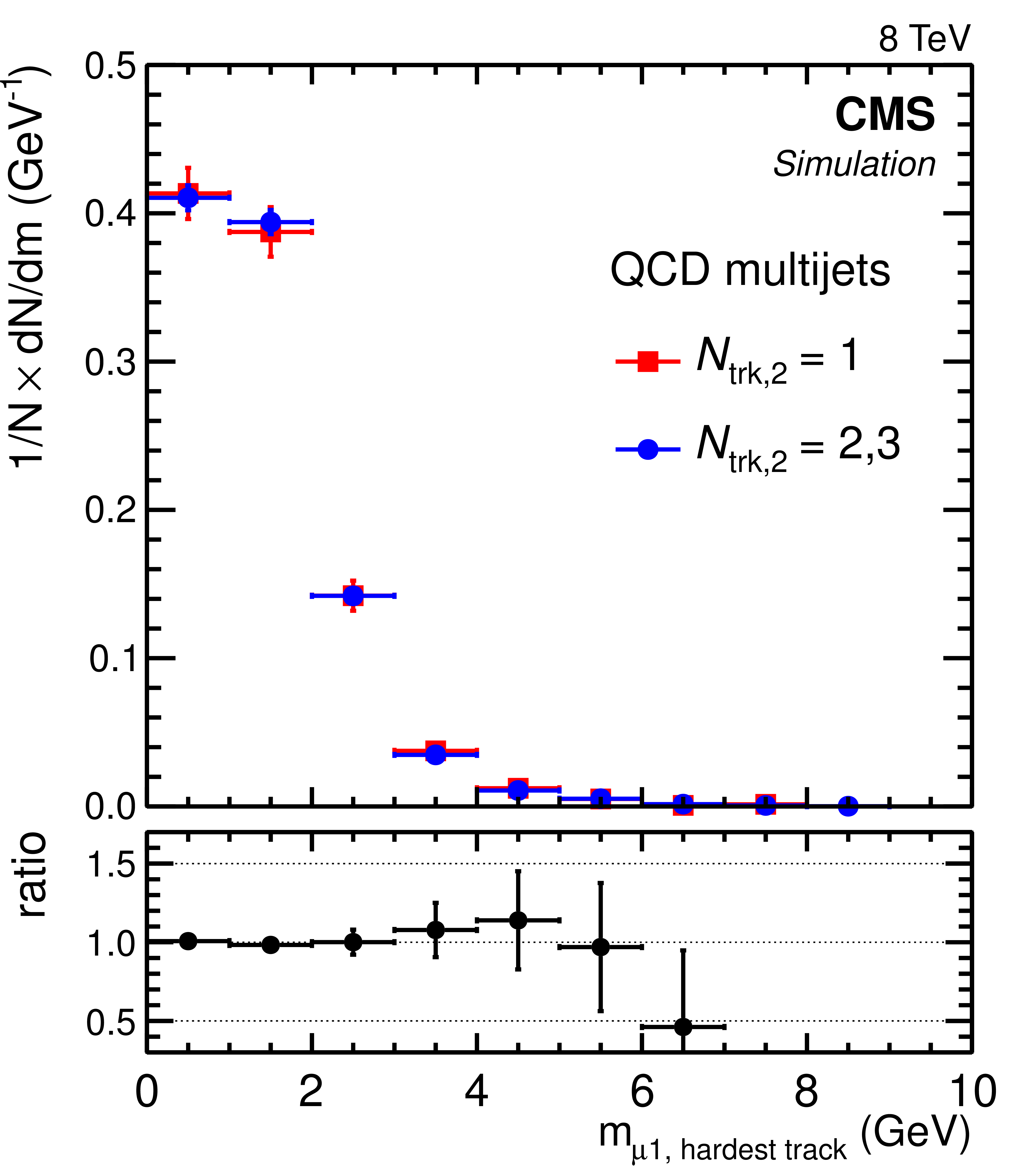
Figure 3-a:
Normalized invariant mass distributions of the first muon and the softest (a,c plots) or hardest (b,d plots) accompanying track for different isolation requirements imposed on the second muon: when the second muon has only one accompanying track ($N_\mathrm {trk,2}=1$; squares); or when the second muon has two or three accompanying tracks ($N_\mathrm {trk,2}=2,3$; circles). The upper plots show distributions obtained from data. The lower plots show distributions obtained from the sample of QCD multijet events generated with PYTHIA. Lower panels in each plot show the ratio of the $N_\mathrm {trk,2}=1$ distribution to the $N_\mathrm {trk,2}=2,3$ distribution. |

png pdf |
Figure 3-b:
Normalized invariant mass distributions of the first muon and the softest (a,c plots) or hardest (b,d plots) accompanying track for different isolation requirements imposed on the second muon: when the second muon has only one accompanying track ($N_\mathrm {trk,2}=1$; squares); or when the second muon has two or three accompanying tracks ($N_\mathrm {trk,2}=2,3$; circles). The upper plots show distributions obtained from data. The lower plots show distributions obtained from the sample of QCD multijet events generated with PYTHIA. Lower panels in each plot show the ratio of the $N_\mathrm {trk,2}=1$ distribution to the $N_\mathrm {trk,2}=2,3$ distribution. |
png pdf |
Figure 3-c:
Normalized invariant mass distributions of the first muon and the softest (a,c plots) or hardest (b,d plots) accompanying track for different isolation requirements imposed on the second muon: when the second muon has only one accompanying track ($N_\mathrm {trk,2}=1$; squares); or when the second muon has two or three accompanying tracks ($N_\mathrm {trk,2}=2,3$; circles). The upper plots show distributions obtained from data. The lower plots show distributions obtained from the sample of QCD multijet events generated with PYTHIA. Lower panels in each plot show the ratio of the $N_\mathrm {trk,2}=1$ distribution to the $N_\mathrm {trk,2}=2,3$ distribution. |
png pdf |
Figure 3-d:
Normalized invariant mass distributions of the first muon and the softest (a,c plots) or hardest (b,d plots) accompanying track for different isolation requirements imposed on the second muon: when the second muon has only one accompanying track ($N_\mathrm {trk,2}=1$; squares); or when the second muon has two or three accompanying tracks ($N_\mathrm {trk,2}=2,3$; circles). The upper plots show distributions obtained from data. The lower plots show distributions obtained from the sample of QCD multijet events generated with PYTHIA. Lower panels in each plot show the ratio of the $N_\mathrm {trk,2}=1$ distribution to the $N_\mathrm {trk,2}=2,3$ distribution. |
png pdf |
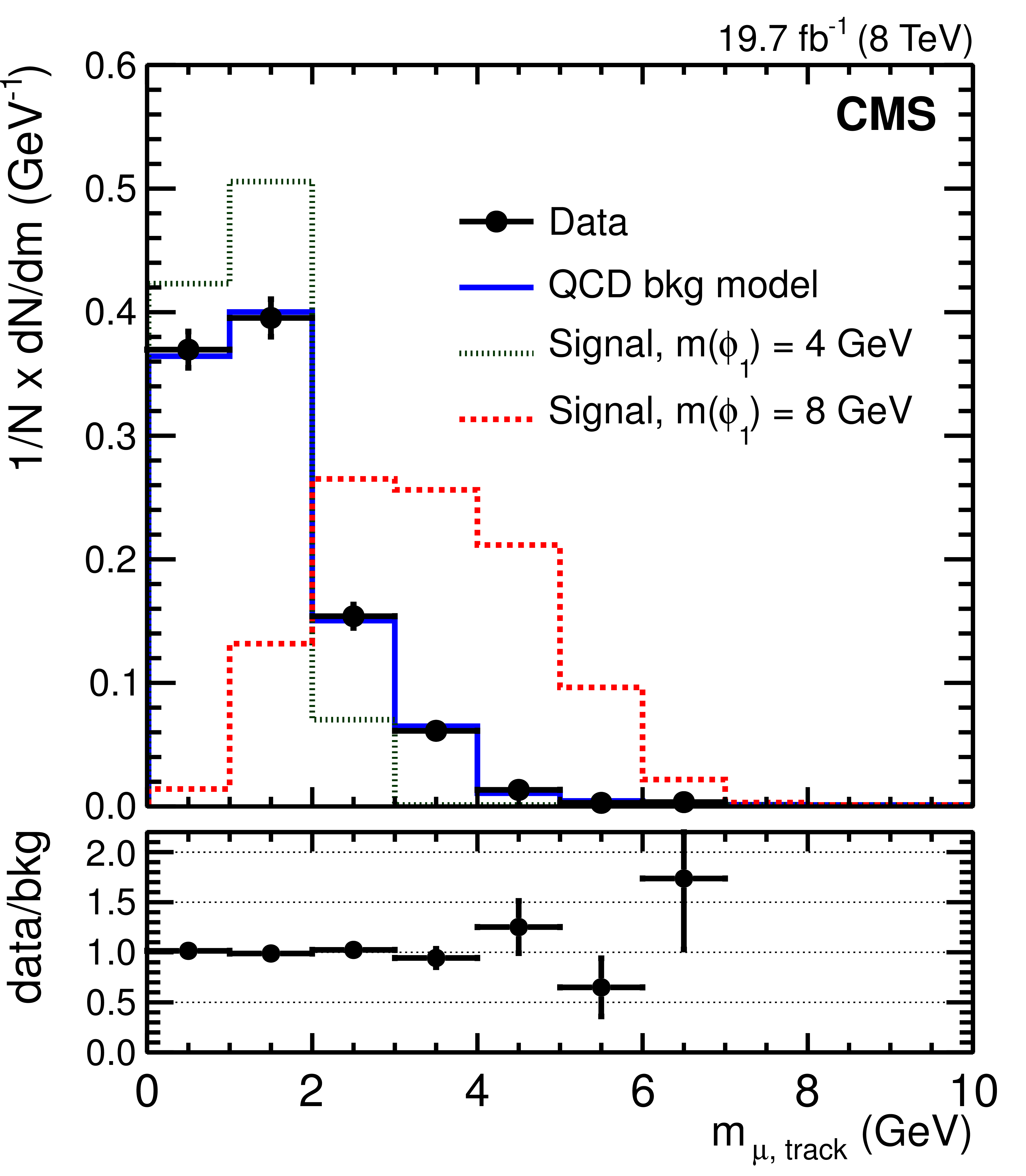
Figure 4:
Normalized invariant mass distribution of the muon-track system for events passing the signal selection. Data are represented by points. The QCD multijet background model is derived from the control region {\bf {N$_{23}$}}. Also shown are the normalized distributions from signal simulations for two mass hypotheses, $m_{\phi _1}=$ 4 GeV (dotted histogram) and 8 GeV (dashed histogram). Each event contributes two entries to the distribution, corresponding to the two muon-track systems passing the selection requirements. The lower panel shows the ratio of the distribution observed in data to the distribution, describing the background model. |
png pdf |
Figure 5:
The ($m_1,m_2$) correlation coefficients $C(i,j)$ along with their statistical uncertainties, derived from data in the control region {\bf {A}}. |
png pdf |
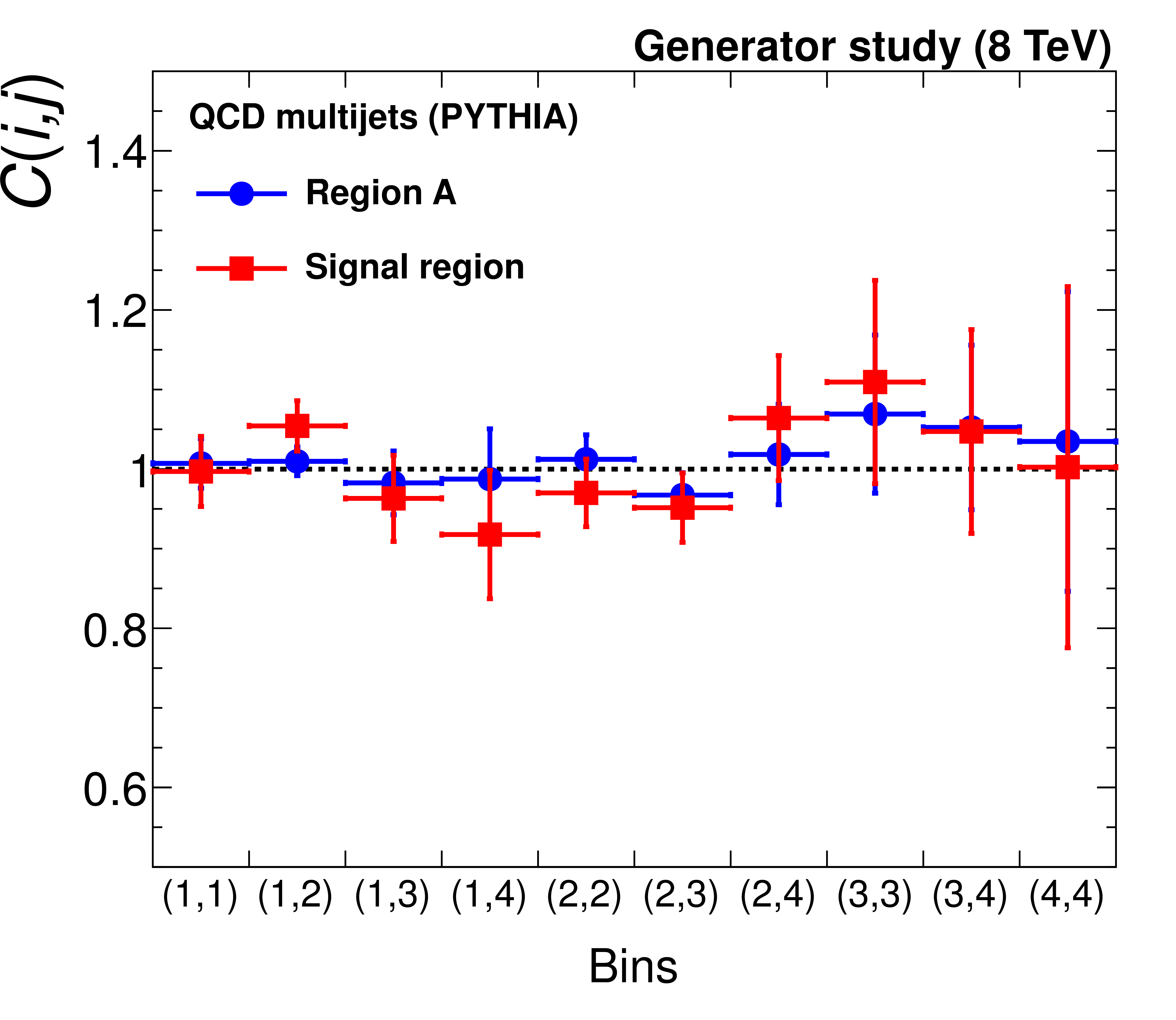
Figure 6:
The ($m_1,m_2$) correlation coefficients $C(i,j)$ determined in the control region {\bf {A}} (circles) and in the signal region (squares) from the MC study carried out at generator level with the exclusive MC sample of QCD multijet events resulting from $ {\mathrm {g}} {\mathrm {g}} ( {\mathrm {q}} {\mathrm {\overline {q}}}) \to { {\mathrm {b}} {\overline {\mathrm {b}}} } $ production mechanisms. The bin notation follows the definition presented in Fig. {fig:binning}. The vertical bars include both statistical and systematic uncertainties. |
png pdf |
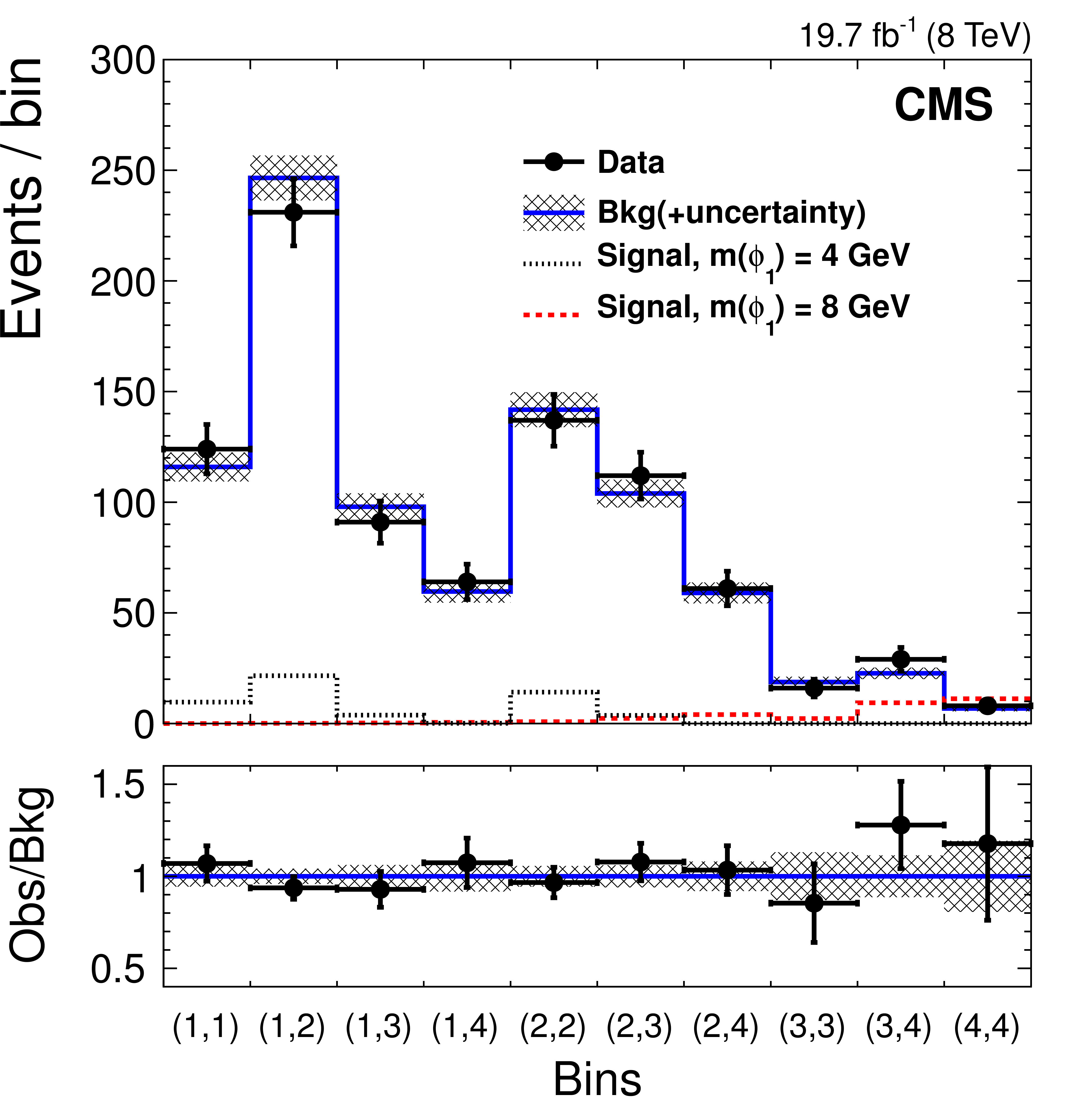
Figure 7-a:
The two-dimensional ($m_1,m_2$) distribution unrolled into a one-dimensional array of analysis bins. In the (a) plot, data (points) are compared with the background prediction (solid histogram) after applying the maximum-likelihood fit under the background-only hypothesis and with the signal expectation for two mass hypotheses, $m_{\phi _{1}}=$ 4 and 8 GeV (dotted and dashed histograms, respectively). The signal distributions are obtained from simulation and normalized to a value of the cross section times branching fraction of 5 pb. In the right plot, data (points) are compared with the background prediction (solid histogram) and the background+signal prediction for $m_{\phi _{1}}=$ 8 GeV (dashed histogram) after applying the maximum-likelihood fit under the signal+background hypothesis. The bin notation follows the definition presented in Fig.2. |
png pdf |
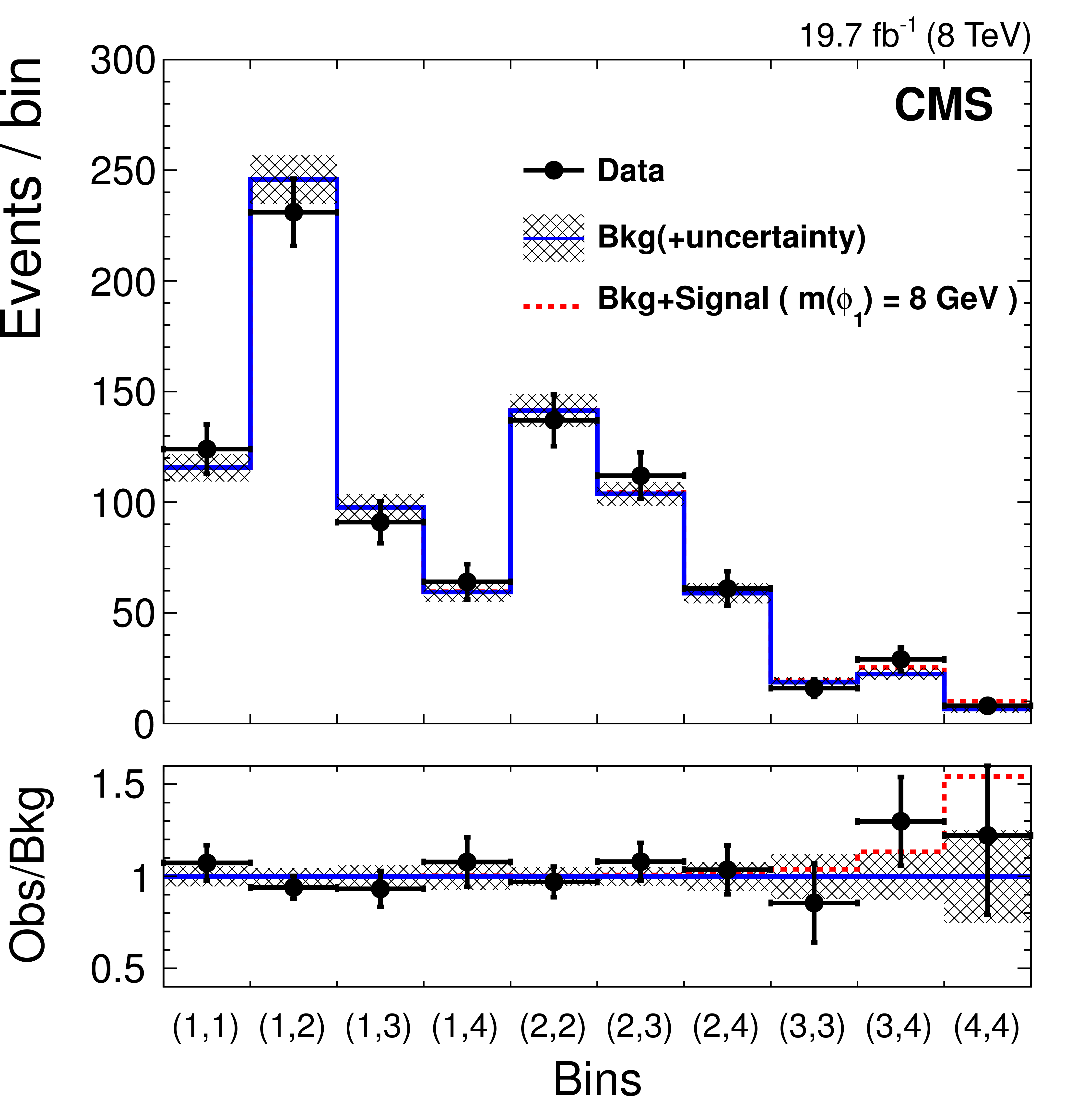
Figure 7-b:
The two-dimensional ($m_1,m_2$) distribution unrolled into a one-dimensional array of analysis bins. In the (a) plot, data (points) are compared with the background prediction (solid histogram) after applying the maximum-likelihood fit under the background-only hypothesis and with the signal expectation for two mass hypotheses, $m_{\phi _{1}}=$ 4 and 8 GeV (dotted and dashed histograms, respectively). The signal distributions are obtained from simulation and normalized to a value of the cross section times branching fraction of 5 pb. In the right plot, data (points) are compared with the background prediction (solid histogram) and the background+signal prediction for $m_{\phi _{1}}=$ 8 GeV (dashed histogram) after applying the maximum-likelihood fit under the signal+background hypothesis. The bin notation follows the definition presented in Fig.2. |

png pdf |
Figure 8:
The observed and expected upper limits on $ {(\sigma \mathcal {B})_\text {sig}}$ in pb at 95% CL, as a function of $m_{\phi _1}$. The expected limit is obtained under the background-only hypothesis. The bands show the expected ${\pm} 1\sigma $ and ${\pm} 2\sigma $ probability intervals around the expected limit. |
| Tables | |

png pdf |
Table 1:
The number of observed events, expected background and signal yields, and signal acceptances after final selection. The computed signal acceptances include the branching fraction factor $\mathcal {B}^{2}(\phi _{1} \to {\tau }_ {{\mu }} {\tau }_\text {one-prong})/2$. The electroweak background contribution includes the Drell--Yan process, $ {\mathrm {W}}+\mathrm {jets}$ production, and diboson production of WW, WZ, and ZZ. The numbers of signal events are reported for the benchmark value of the signal production cross section times branching fraction of 5 pb. The expected background and signal yields and signal acceptances are obtained from simulation. The quoted uncertainties in predictions from simulation include only statistical uncertainties related to the size of MC samples. |
png pdf |
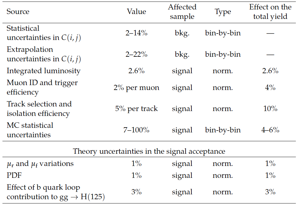
Table 2:
Systematic uncertainties and their effect on the estimates of the QCD multijet background and signal. The effect of the uncertainties in $C(i,j)$ on the total background yield is absorbed by the overall background normalization, which is allowed to vary freely in the fit. |
png pdf |
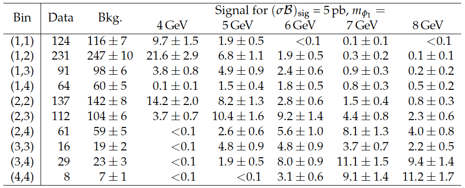
Table 3:
The number of observed data events, the predicted background yields, and the expected signal yields, for different masses of the $\phi _1$ boson in individual bins of the ($m_1,m_2$) distribution. The background yields and uncertainties are obtained from the maximum-likelihood fit under the background-only hypothesis. The signal yields are obtained from simulation and normalized to a signal cross section times branching fraction of 5 pb. The uncertainties in the signal yields include systematic and MC statistical uncertainties. The bin notation follows the definition presented in Fig.2. |

png pdf |
Table 4:
The observed upper limit on $ {(\sigma \mathcal {B})_\text {sig}}$ at 95% CL, together with the expected limit obtained in the background-only hypothesis, as a function of $m_{\phi _1}$. Also shown are ${\pm}1\sigma $ and ${\pm}2\sigma $ probability intervals around the expected limit. |
| Summary |
| A search for a very light NMSSM Higgs boson $\mathrm{ a_1 }$ or $\mathrm{ h_1 }$, produced in decays of the observed boson with a mass near 125 GeV, $\mathrm{ H(125) }$, is performed on a pp collision data set corresponding to an integrated luminosity of 19.7 fb$^{-1}$, collected at a centre-of-mass energy of 8 TeV. The analysis searches for the production of an $\mathrm{ H(125) }$ boson via gluon-gluon fusion, and its decay into a pair of $\mathrm{ a_1 }$ $(\mathrm{ h_1 })$ states, each of which decays into a pair of $\tau$ leptons. The search covers a mass range of the $\mathrm{ a_1 }$ $(\mathrm{ h_1 })$ boson of 4 to 8 GeV. No significant excess above background expectations is found in data, and upper limits at 95% CL are set on the signal production cross section times branching fraction,$(\sigma \mathcal{B})_\text{sig} \equiv \sigma (\mathrm{gg} \to \mathrm{ H(125) }) \, \mathcal{B} (\mathrm{ H(125) } \to \phi_1 \phi_1) \, \mathcal{B}^{2} (\phi_1 \to \tau\tau)$,where $\phi_1$ is either the $\mathrm{ a_1 }$ or $\mathrm{ h_1 }$ boson. The observed upper limit at 95% CL on $(\sigma \mathcal{B})_\text{sig}$ ranges from 4.5 pb at $m_{\phi_1}= $ 8 GeV to 10.3 pb at $m_{\phi_1} =$ 5 GeV. |
|
|
Compact Muon Solenoid LHC, CERN |
|

|

|

|

|

|