

Compact Muon Solenoid
LHC, CERN
| CMS-HIG-14-023 ; CERN-PH-EP-2015-221 | ||
| Search for a charged Higgs boson in pp collisions at $\sqrt{s} =$ 8 TeV | ||
| CMS Collaboration | ||
| 31 August 2015 | ||
| J. High Energy Phys. 11 (2015) 018 | ||
| Abstract: A search for a charged Higgs boson is performed with a data sample corresponding to an integrated luminosity of 19.7 $\pm$ 0.5 fb$^{-1}$ collected with the CMS detector in proton-proton collisions at $\sqrt{s} =$ 8 TeV. The charged Higgs boson is searched for in top quark decays for $ m_{\mathrm{H}^\pm} < m_{\mathrm t} - m_{\mathrm b}$, and in the direct production ${\rm pp \rightarrow t (b) H^\pm}$ for $m_{\mathrm H^\pm} > m_{\mathrm t} - m_{\mathrm b}$. The ${\mathrm H^\pm\rightarrow \tau^\pm\nu_\tau}$ and ${\rm H^\pm\rightarrow t b}$ decay modes in the final states $\tau_{\rm h}$+jets, $\mu\tau_{\rm h}$, $\ell$+jets, and $\ell\ell$' ($\ell =$ e, $\mu$) are considered in the search. No signal is observed and 95% confidence level upper limits are set on the charged Higgs boson production. A model-independent upper limit on the product branching fraction $\mathcal{B}({\rm t\rightarrow H^\pm b}) \, \mathcal{B}({\mathrm H^\pm \rightarrow \tau^\pm \nu_\tau})= $ 1.2-0.15% is obtained in the mass range $m_{\mathrm H^\pm} =$ 80-160 GeV, while the upper limit on the cross section times branching fraction $\sigma({\rm pp \rightarrow t (b) H^\pm}) \, \mathcal{B} ({\mathrm H^\pm \rightarrow \tau^\pm \nu_\tau})=$ 0.38-0.025 pb is set in the mass range $m_{\mathrm H^+} =$ 180-600 GeV. Here, cross section $\sigma({\rm pp} \to {\rm t(b)H}^{\pm})$ stands for the sum $\sigma({\rm pp} \to \overline{\rm t}({\rm b}){\rm H}^{+}) + \sigma({\rm pp} \to {\rm t}(\overline{\rm b}){\rm H}^{-})$. Assuming $\mathcal{B}({\rm H}^\pm \rightarrow {\rm t b})=$ 1, an upper limit on $\sigma ({\rm pp} \rightarrow {\rm t} ({\rm b}) {\rm H}^\pm)$ of 2.0-0.13 pb is set for $m_{\mathrm H^\pm} =$ 180-600 GeV. The combination of all considered decay modes and final states is used to set exclusion limits in the $m_{\mathrm H^\pm}$-$\tan\beta$ parameter space in different MSSM benchmark scenarios. | ||
| Links: e-print arXiv:1508.07774 [hep-ex] (PDF) ; CDS record ; inSPIRE record ; CADI line (restricted) ; | ||
| Figures | |
png pdf |
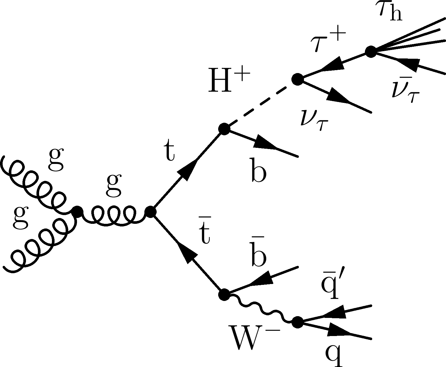
Figure 1-a:
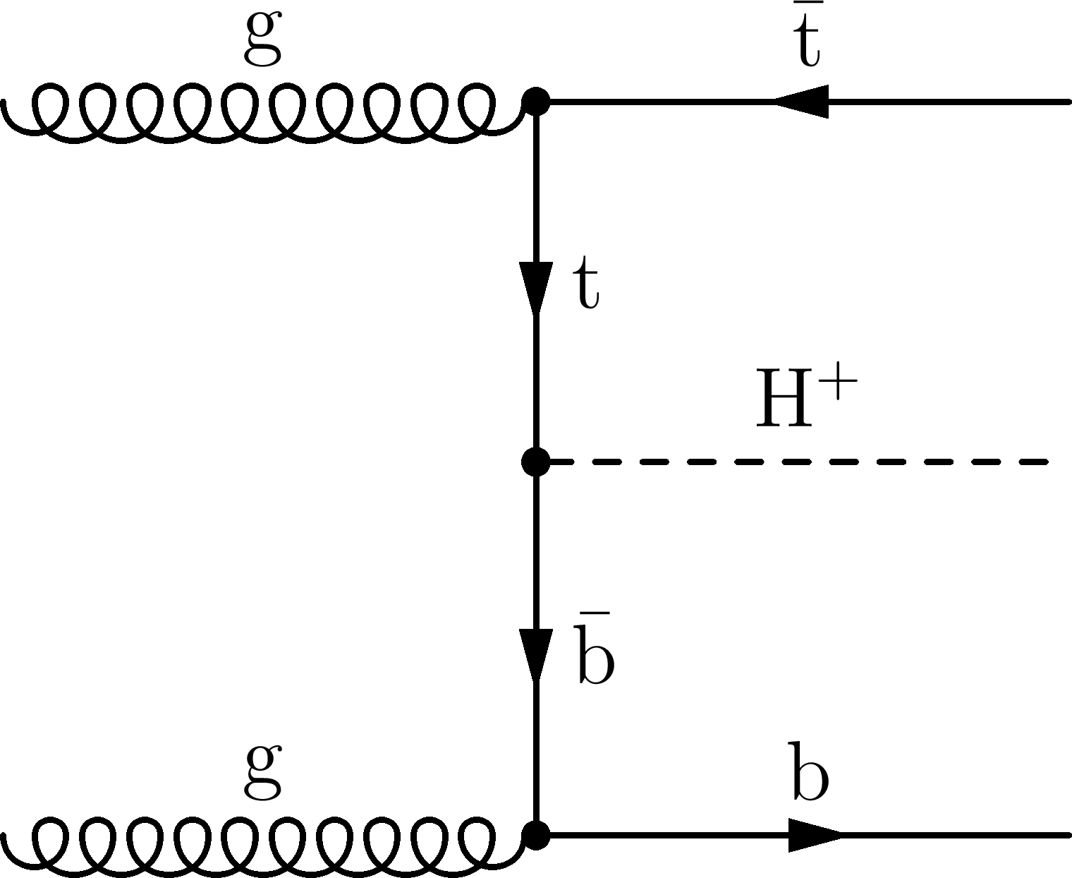
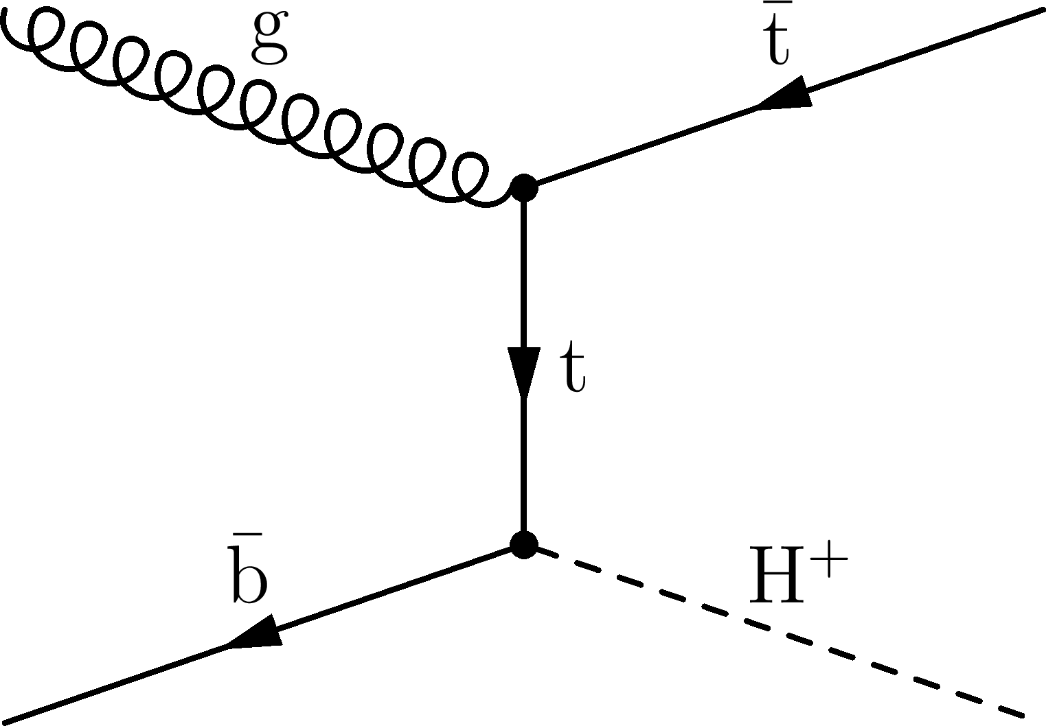
(a) A representative diagram for the production mode of the light charged Higgs boson through $ {\mathrm {t}\overline {\mathrm {t}}} $ production with a subsequent decay to the $ { { {\tau }_{\mathrm {h}}} }$+jets final state. (c,d) Representative diagrams for the direct production of the charged Higgs boson in the four-flavour scheme and five-flavour scheme, respectively. |
png pdf |
Figure 1-b:
(a) A representative diagram for the production mode of the light charged Higgs boson through $ {\mathrm {t}\overline {\mathrm {t}}} $ production with a subsequent decay to the $ { { {\tau }_{\mathrm {h}}} }$+jets final state. (c,d) Representative diagrams for the direct production of the charged Higgs boson in the four-flavour scheme and five-flavour scheme, respectively. |
png pdf |
Figure 1-c:
(a) A representative diagram for the production mode of the light charged Higgs boson through $ {\mathrm {t}\overline {\mathrm {t}}} $ production with a subsequent decay to the $ { { {\tau }_{\mathrm {h}}} }$+jets final state. (c,d) Representative diagrams for the direct production of the charged Higgs boson in the four-flavour scheme and five-flavour scheme, respectively. |

png pdf |
Figure 2:
The event yield in the $ { { {\tau }_{\mathrm {h}}} }$+jets final state after each selection step. For illustrative purposes, the expected signal yields are shown for $ {m_{ {\mathrm {H}} ^+}} =$ 120 GeV normalized to $ { {\mathcal {B}( { {\mathrm {t}}\to {\mathrm {H}} ^{+} {\mathrm {b}}} )} \, {\mathcal {B}( { {\mathrm {H}} ^{+}\to {\tau }^{+} {\nu _{\tau }}} )} } =$ 0.01 and for $ {m_{ {\mathrm {H}} ^+}} = $ 300 GeV normalized to $ { {\sigma ({ {\mathrm {p}} {\mathrm {p}}\to {\overline {\mathrm {t}}}( {\mathrm {b}}) {\mathrm {H}} ^{+}})} \, {\mathcal {B}( { {\mathrm {H}} ^{+}\to {\tau }^{+} {\nu _{\tau }}} )} } =$ 1 pb, which are typical values for the sensitivity of this analysis. The bottom panel shows the ratio of data over the sum of expected backgrounds and its uncertainties. The cross-hatched (light grey) area in the upper (lower) part of the figure represents the statistical uncertainty, while the collinear-hatched (dark grey) area gives the total uncertainty in the background expectation. |
png pdf |
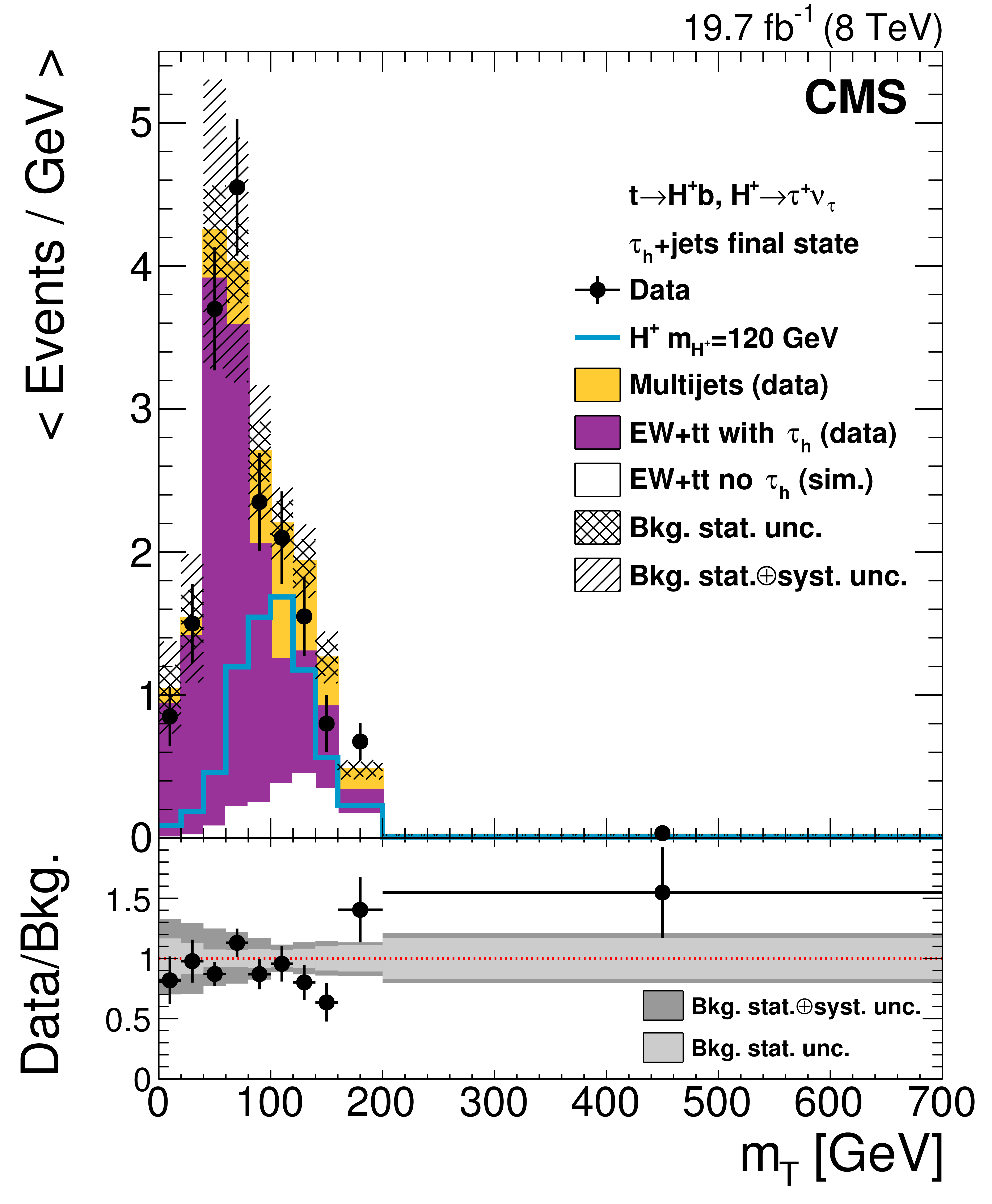
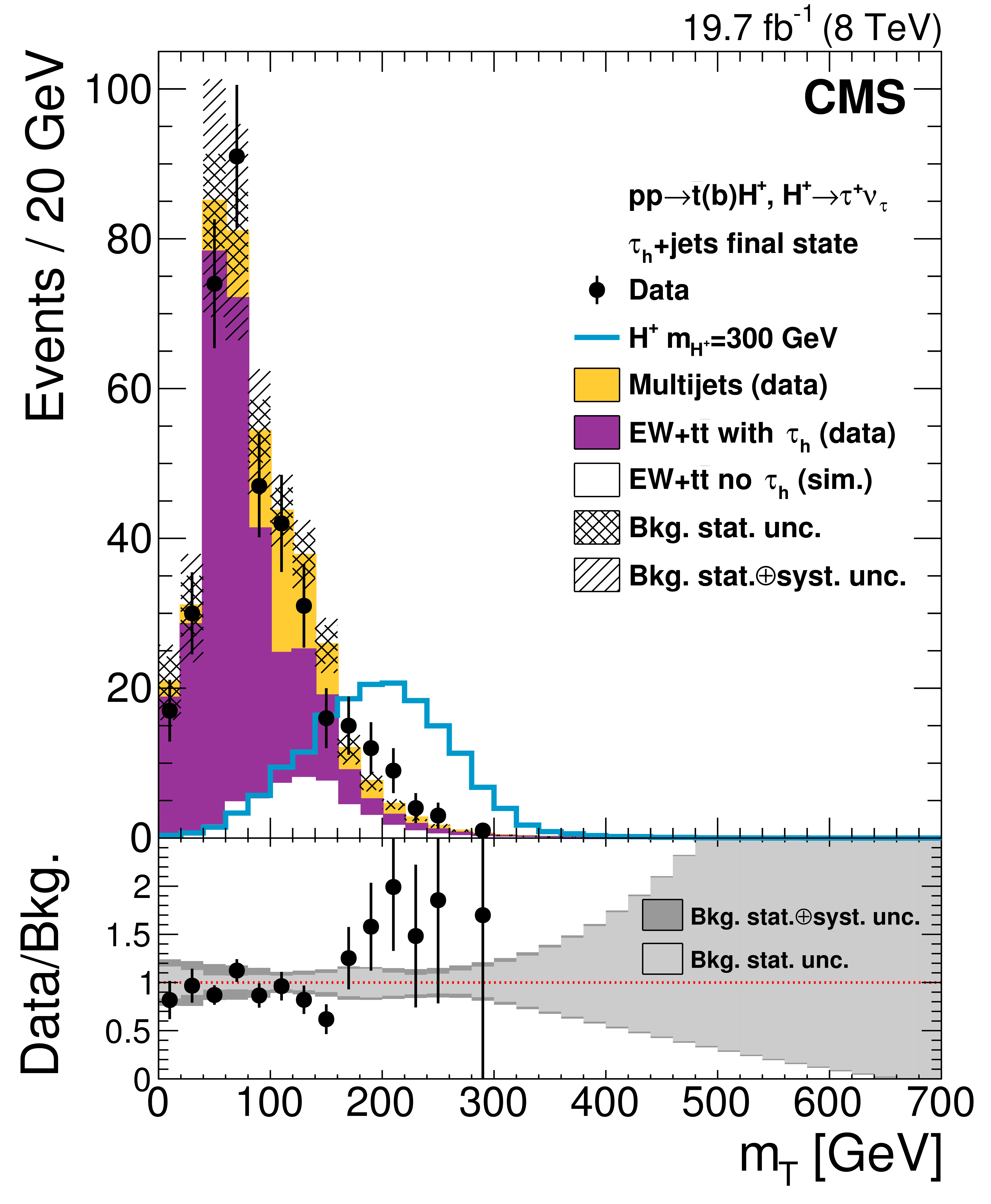
Figure 3-a:
The transverse mass ($ {m_\mathrm {T}} $) distributions in the $ { { {\tau }_{\mathrm {h}}} }$+jets final state for the $ {\mathrm {H}} ^+$ mass hypotheses of (a) 80--160 GeV and (b) 180--600 GeV. The event selection is the same in both (a) and (b), but in (b) the background expectation is replaced for $ {m_\mathrm {T}} >$ 160 GeV by a fit of the falling part of the $ {m_\mathrm {T}} $ distribution. Since a variable bin width is used in (a) the event yield in each bin has been divided by the bin width. For illustrative purposes, the expected signal yields are shown for (a) $ {m_{ {\mathrm {H}} ^+}} = $ 120 GeV normalized to $ { {\mathcal {B}( { {\mathrm {t}}\to {\mathrm {H}} ^{+} {\mathrm {b}}} )} \, {\mathcal {B}( { {\mathrm {H}} ^{+}\to {\tau }^{+} {\nu _{\tau }}} )} } =$ 0.01 and for (b) $ {m_{ {\mathrm {H}} ^+}} = 300$ GeV normalized to $ { {\sigma ({ {\mathrm {p}} {\mathrm {p}}\to {\overline {\mathrm {t}}}( {\mathrm {b}}) {\mathrm {H}} ^{+}})} \times {\mathcal {B}( { {\mathrm {H}} ^{+}\to {\tau }^{+} {\nu _{\tau }}} )} } = 1$ pb, which are typical values for the sensitivity of this analysis. The bottom panel shows the ratio of data over the sum of expected backgrounds along with the uncertainties. The cross-hatched (light grey) area in the upper (lower) part of the figure represents the statistical uncertainty, while the collinear-hatched (dark grey) area gives the total uncertainty in the background expectation. |
png pdf |
Figure 3-b:
The transverse mass ($ {m_\mathrm {T}} $) distributions in the $ { { {\tau }_{\mathrm {h}}} }$+jets final state for the $ {\mathrm {H}} ^+$ mass hypotheses of (a) 80--160 GeV and (b) 180--600 GeV. The event selection is the same in both (a) and (b), but in (b) the background expectation is replaced for $ {m_\mathrm {T}} >$ 160 GeV by a fit of the falling part of the $ {m_\mathrm {T}} $ distribution. Since a variable bin width is used in (a) the event yield in each bin has been divided by the bin width. For illustrative purposes, the expected signal yields are shown for (a) $ {m_{ {\mathrm {H}} ^+}} = $ 120 GeV normalized to $ { {\mathcal {B}( { {\mathrm {t}}\to {\mathrm {H}} ^{+} {\mathrm {b}}} )} \, {\mathcal {B}( { {\mathrm {H}} ^{+}\to {\tau }^{+} {\nu _{\tau }}} )} } =$ 0.01 and for (b) $ {m_{ {\mathrm {H}} ^+}} = 300$ GeV normalized to $ { {\sigma ({ {\mathrm {p}} {\mathrm {p}}\to {\overline {\mathrm {t}}}( {\mathrm {b}}) {\mathrm {H}} ^{+}})} \times {\mathcal {B}( { {\mathrm {H}} ^{+}\to {\tau }^{+} {\nu _{\tau }}} )} } = 1$ pb, which are typical values for the sensitivity of this analysis. The bottom panel shows the ratio of data over the sum of expected backgrounds along with the uncertainties. The cross-hatched (light grey) area in the upper (lower) part of the figure represents the statistical uncertainty, while the collinear-hatched (dark grey) area gives the total uncertainty in the background expectation. |
png pdf |
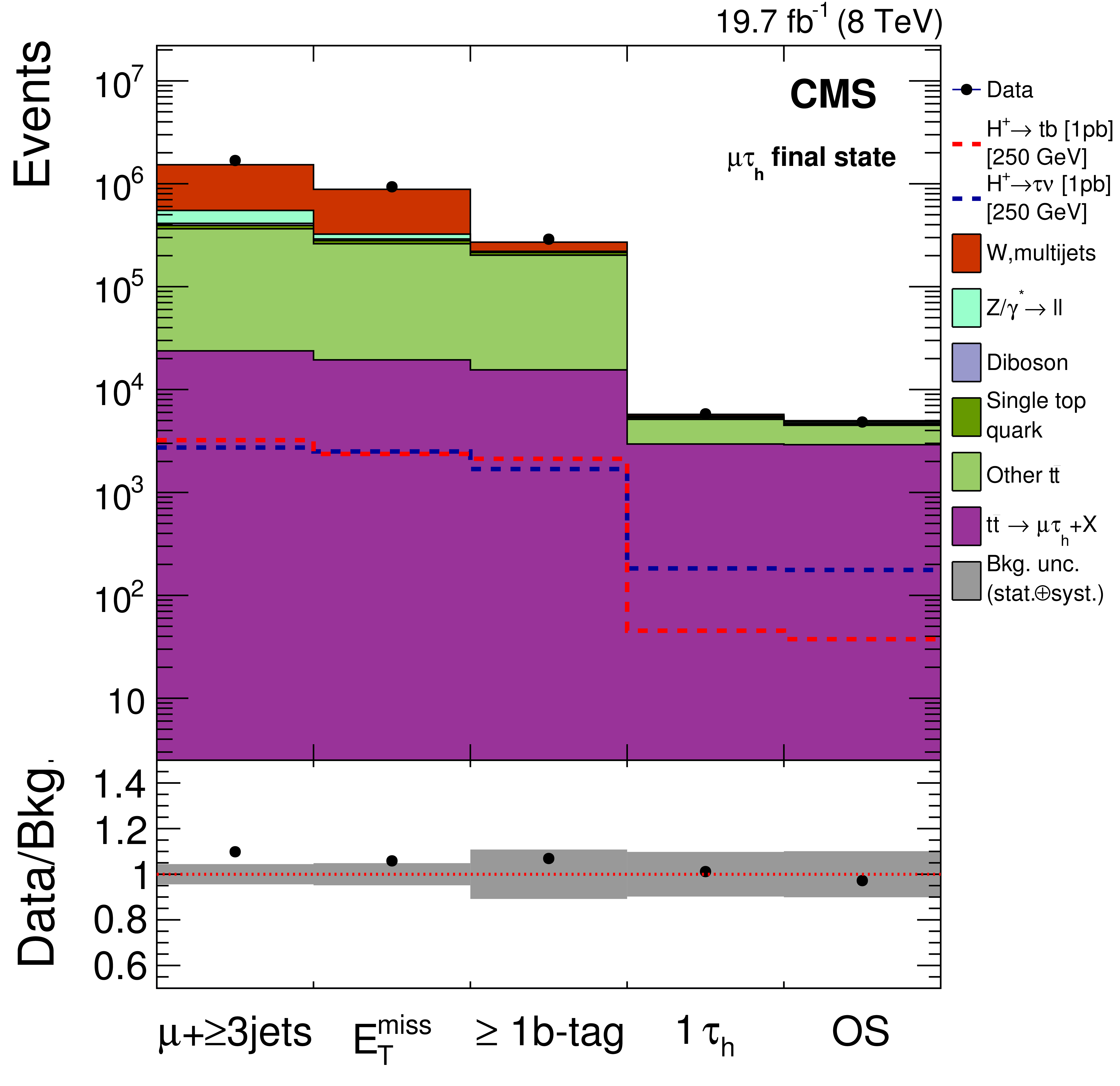
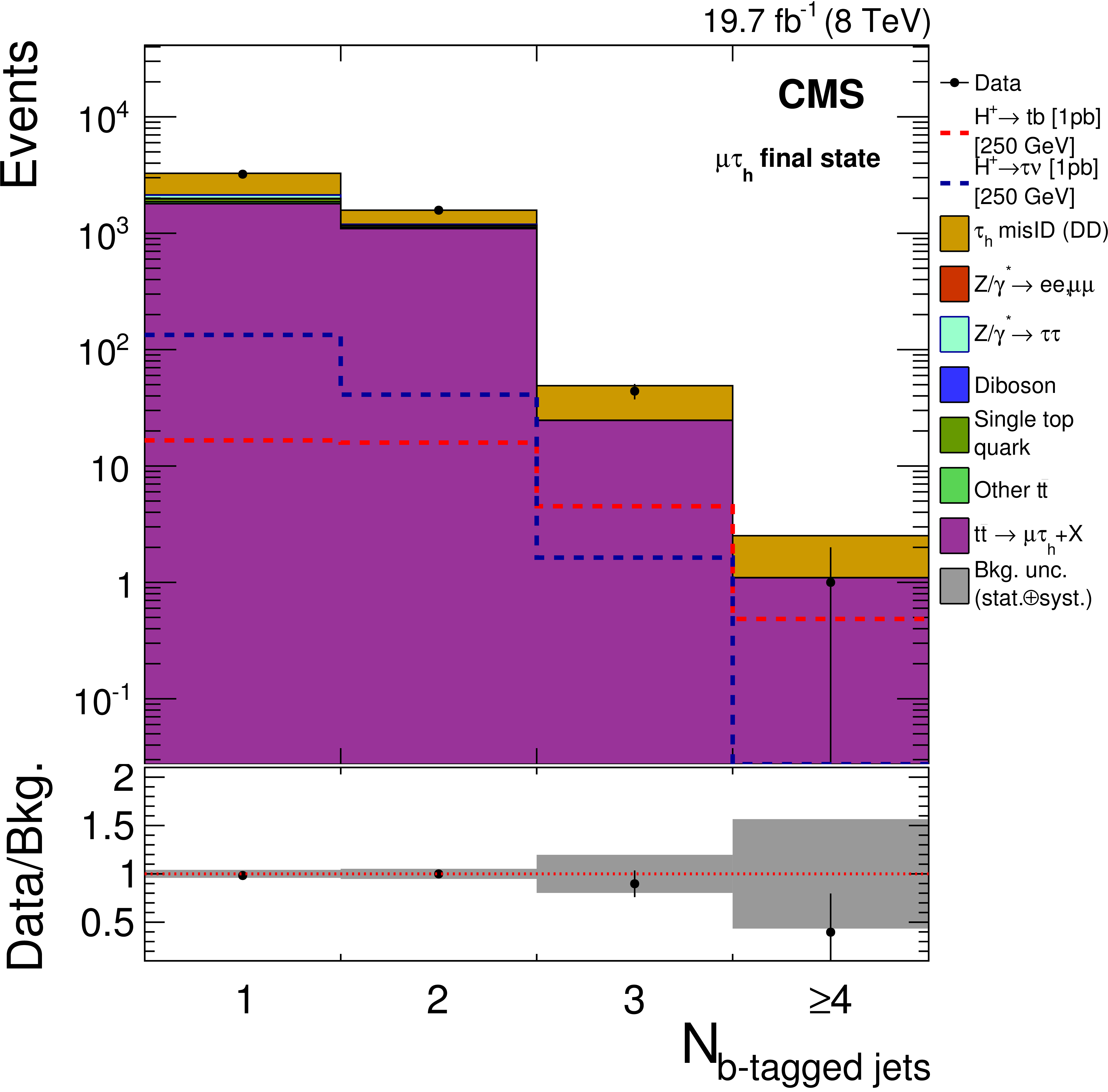
Figure 4-a:
(a) event yields after each selection step, where OS indicates the requirement to have opposite electric charges for the $ {\tau }_\mathrm {h}$ and the $ {{\mu }}$. The backgrounds are estimated from simulation and normalized to the SM prediction. (b) the b-tagged jet multiplicity distribution after the full event selection. As opposed to (a), the ``misidentified $ { {\tau }_{\mathrm {h}}} $'' component is estimated using the data-driven method and labeled ``$ { {\tau }_{\mathrm {h}}} $ misID (DD)``, while the remaining background contributions are from simulation normalized to the SM predicted values. For both distributions, the expected event yield in the presence of the $ { {\mathrm {H}} ^{+}\to {\mathrm {t}} {\overline {\mathrm {b}}}} $ and $ { {\mathrm {H}} ^{+}\to {\tau }^{+} {\nu _{\tau }}} $ decays is shown as dashed lines for $ {m_{ {\mathrm {H}} ^+}} =$ 250 GeV. For illustrative purposes, the number of signal events is normalized, assuming a 100% branching fraction for each decay mode, to a cross section of 1 pb, which is typical of the cross section sensitivity of this analysis. $\mathcal {B}( {\mathrm {H}} ^{+}\to {\mathrm {t}} {\overline {\mathrm {b}}})=$ 1 and $\mathcal {B}( {\mathrm {H}} ^{+}\to {\tau }^{+} {\nu _{\tau }})=$ 1, respectively. The bottom panel shows the ratio of data over the sum of the SM backgrounds; the shaded grey area shows the statistical and systematic uncertainties added in quadrature. |
png pdf |
Figure 4-b:
(a) event yields after each selection step, where OS indicates the requirement to have opposite electric charges for the $ {\tau }_\mathrm {h}$ and the $ {{\mu }}$. The backgrounds are estimated from simulation and normalized to the SM prediction. (b) the b-tagged jet multiplicity distribution after the full event selection. As opposed to (a), the ``misidentified $ { {\tau }_{\mathrm {h}}} $'' component is estimated using the data-driven method and labeled ``$ { {\tau }_{\mathrm {h}}} $ misID (DD)``, while the remaining background contributions are from simulation normalized to the SM predicted values. For both distributions, the expected event yield in the presence of the $ { {\mathrm {H}} ^{+}\to {\mathrm {t}} {\overline {\mathrm {b}}}} $ and $ { {\mathrm {H}} ^{+}\to {\tau }^{+} {\nu _{\tau }}} $ decays is shown as dashed lines for $ {m_{ {\mathrm {H}} ^+}} =$ 250 GeV. For illustrative purposes, the number of signal events is normalized, assuming a 100% branching fraction for each decay mode, to a cross section of 1 pb, which is typical of the cross section sensitivity of this analysis. $\mathcal {B}( {\mathrm {H}} ^{+}\to {\mathrm {t}} {\overline {\mathrm {b}}})=$ 1 and $\mathcal {B}( {\mathrm {H}} ^{+}\to {\tau }^{+} {\nu _{\tau }})=$ 1, respectively. The bottom panel shows the ratio of data over the sum of the SM backgrounds; the shaded grey area shows the statistical and systematic uncertainties added in quadrature. |
png pdf |
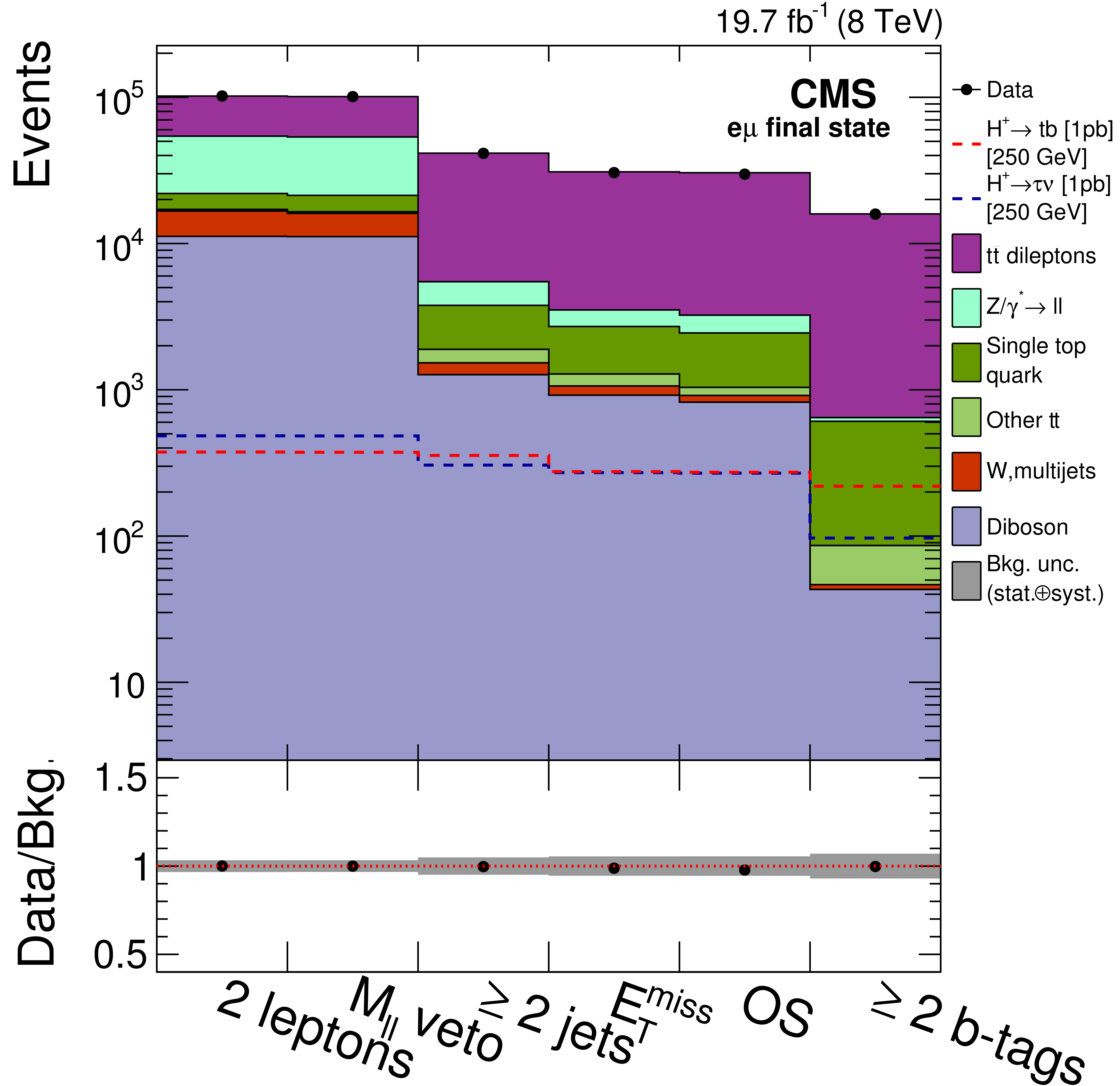
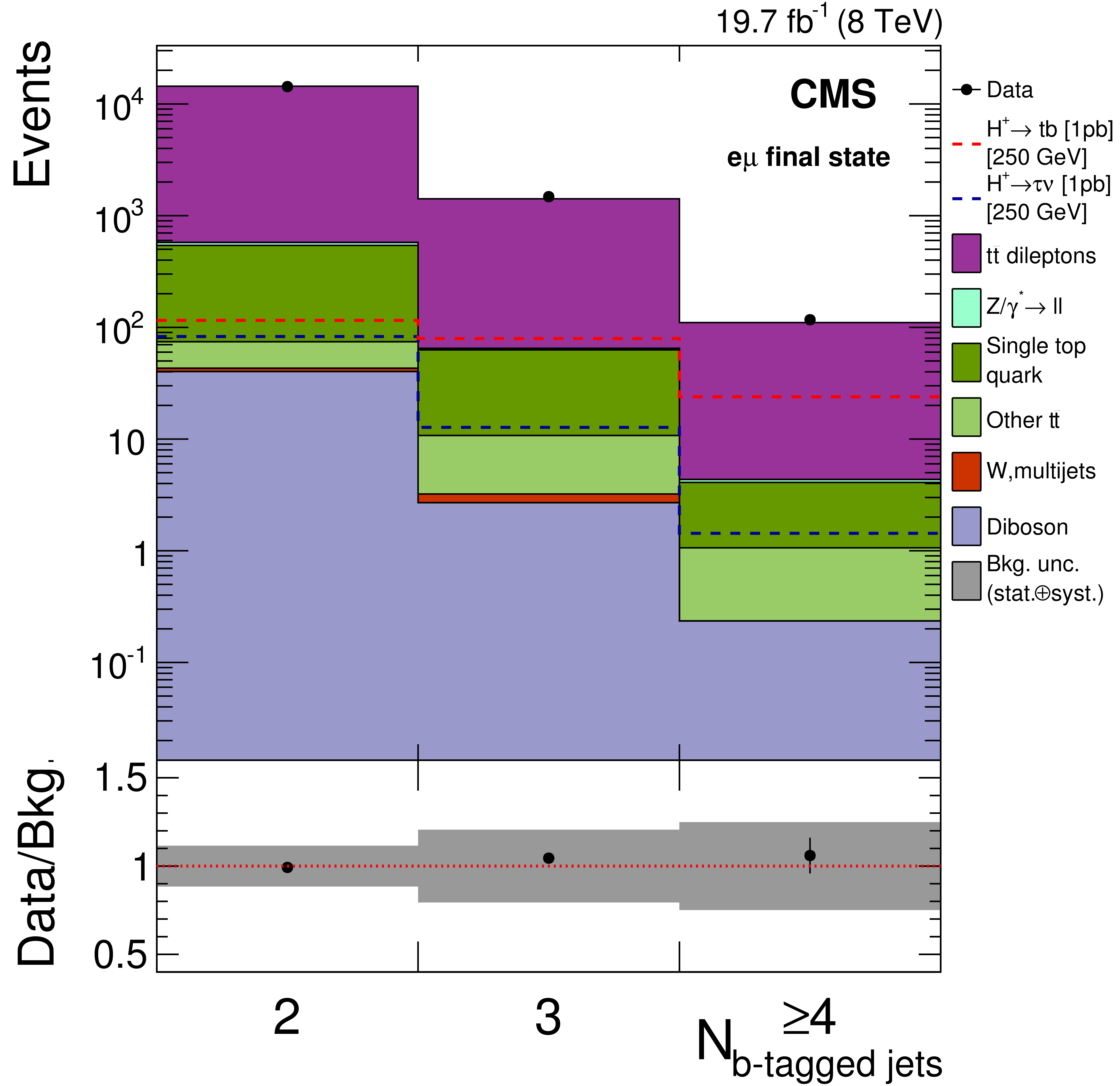
Figure 5-a:
(a) the event yields at different selection steps and (b) the b-tagged jet multiplicity after the full event selection for the $ {\mathrm {e}} {{\mu }}$ final state. For illustrative purposes, the number of signal events is normalized, assuming a 100% branching fraction for each decay mode, to a cross section of 1 pb, which is typical of the cross section sensitivity of this analysis. The bottom panel shows the ratio of data over the sum of the SM backgrounds; the shaded area shows the statistical and systematic uncertainties added in quadrature. |
png pdf |
Figure 5-b:
(a) the event yields at different selection steps and (b) the b-tagged jet multiplicity after the full event selection for the $ {\mathrm {e}} {{\mu }}$ final state. For illustrative purposes, the number of signal events is normalized, assuming a 100% branching fraction for each decay mode, to a cross section of 1 pb, which is typical of the cross section sensitivity of this analysis. The bottom panel shows the ratio of data over the sum of the SM backgrounds; the shaded area shows the statistical and systematic uncertainties added in quadrature. |
png pdf |
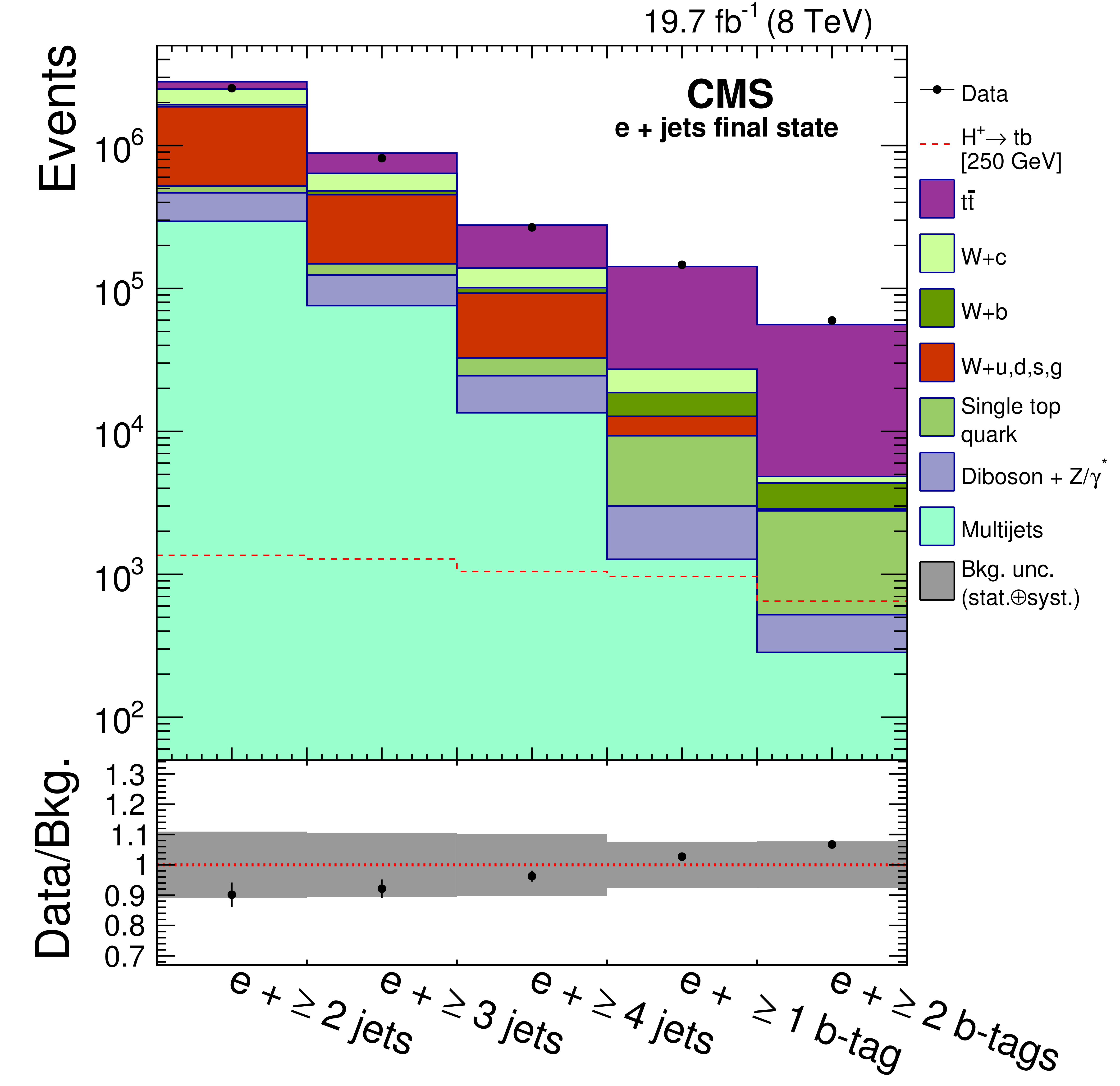
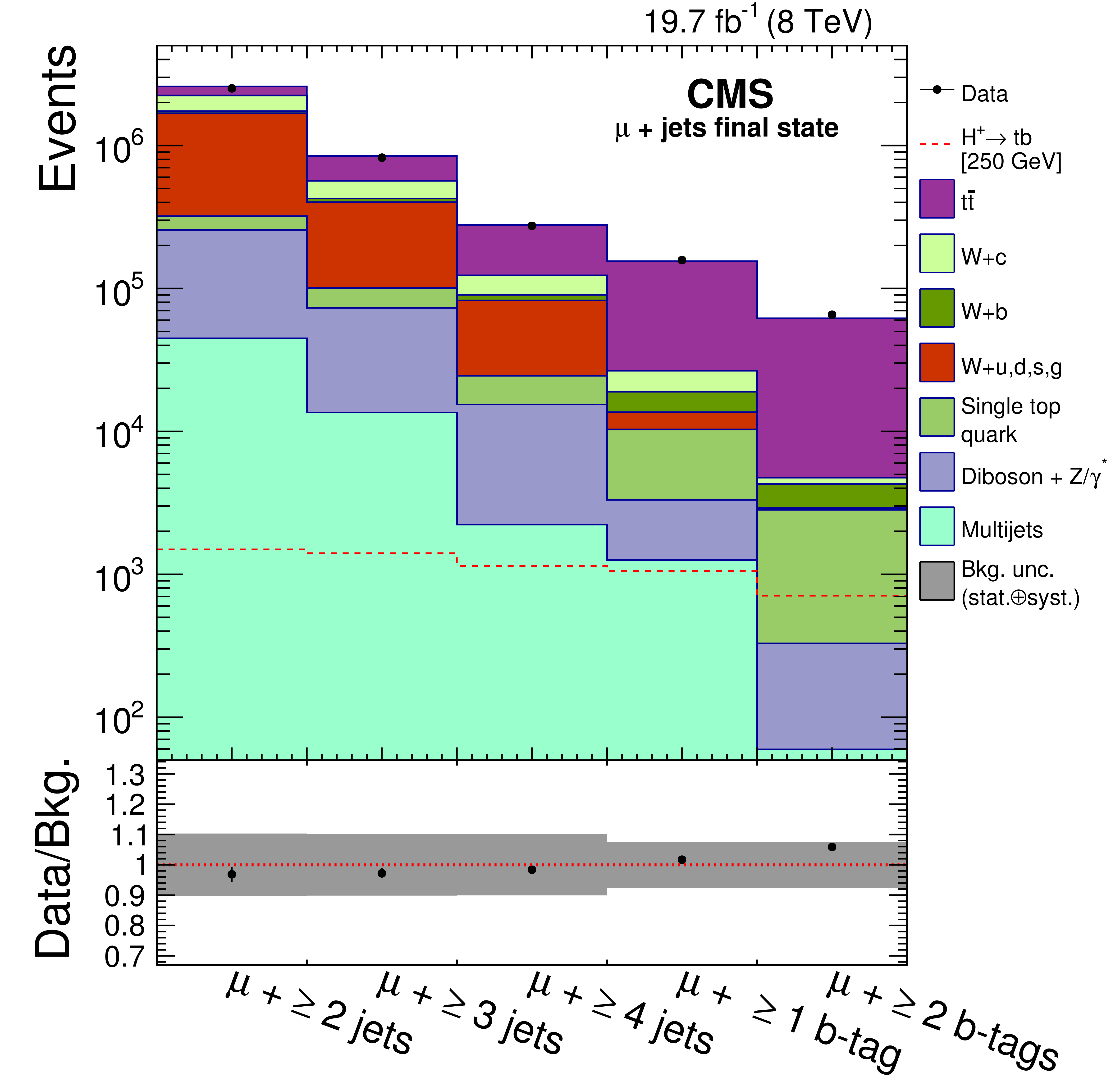
Figure 6-a:
Event yields after different selection cuts for both the (a) $ {\mathrm {e}}$+jets and (b) $ {{\mu }}$+jets final state. Expectations for the charged Higgs boson for $ {m_{ {\mathrm {H}} ^+}} =$ 250 GeV, for the ${ {\mathrm {H}} ^{+}\to {\mathrm {t}} {\overline {\mathrm {b}}}} $ decays, are also shown. For illustrative purposes, the signal is normalized, assuming $ {\mathcal {B}( { {\mathrm {t}}\to {\mathrm {H}} ^{+} {\mathrm {b}}} )} =$ 1, to a cross section of 1 pb, which is typical of the cross section sensitivity of this analysis. The bottom panel shows the ratio of data over the sum of the SM backgrounds with the total uncertainties. |
png pdf |
Figure 6-b:
Event yields after different selection cuts for both the (a) $ {\mathrm {e}}$+jets and (b) $ {{\mu }}$+jets final state. Expectations for the charged Higgs boson for $ {m_{ {\mathrm {H}} ^+}} =$ 250 GeV, for the ${ {\mathrm {H}} ^{+}\to {\mathrm {t}} {\overline {\mathrm {b}}}} $ decays, are also shown. For illustrative purposes, the signal is normalized, assuming $ {\mathcal {B}( { {\mathrm {t}}\to {\mathrm {H}} ^{+} {\mathrm {b}}} )} =$ 1, to a cross section of 1 pb, which is typical of the cross section sensitivity of this analysis. The bottom panel shows the ratio of data over the sum of the SM backgrounds with the total uncertainties. |
png pdf |
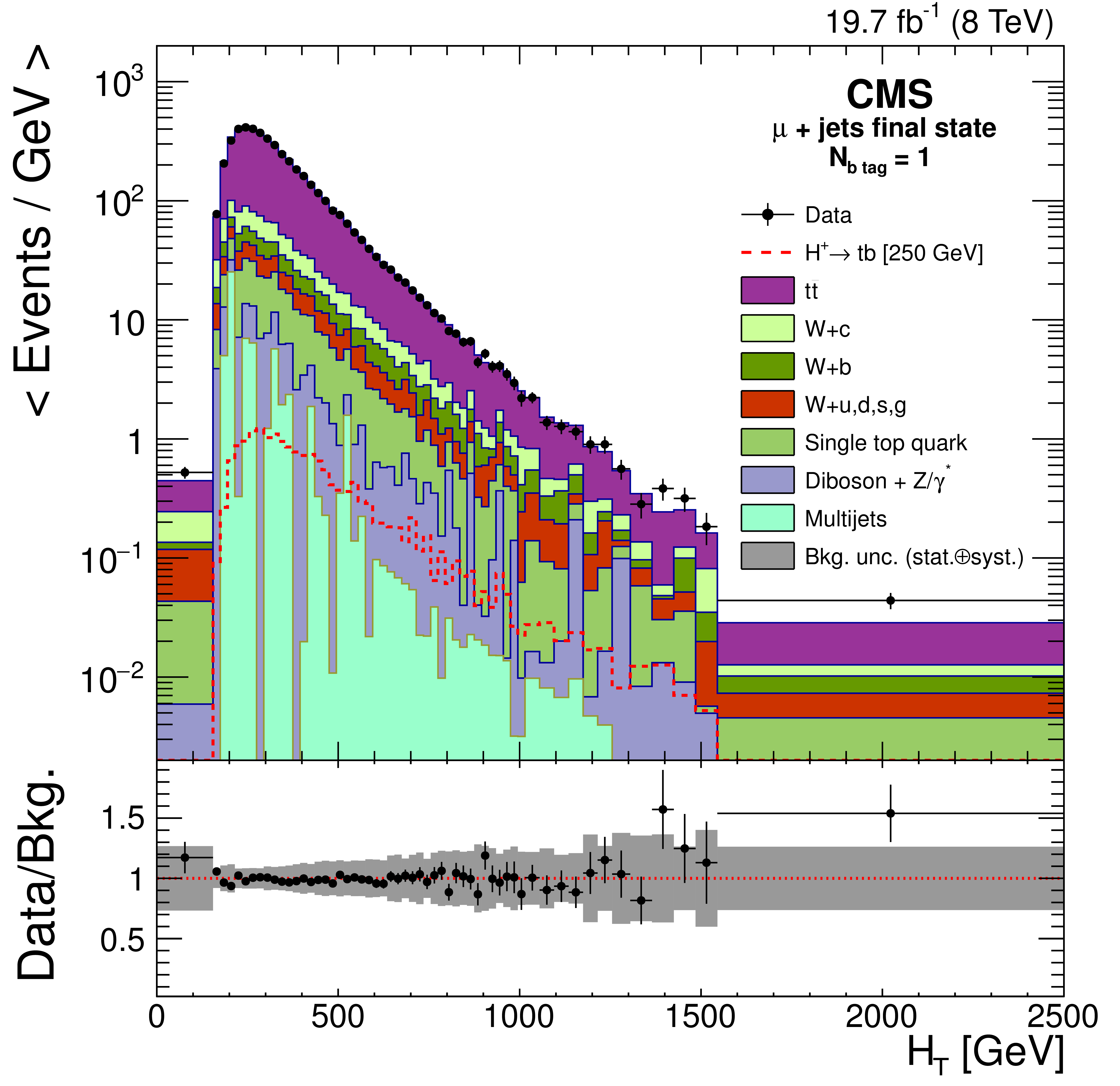
Figure 7-a:
The $ {H_{\mathrm {T}}} $ distributions observed in data and predicted for signal and background in the $ {{\mu }}$+jets channel with (a) $N_\mathrm {btag}=$ 1 and (b) $N_\mathrm {btag}\geq$ 2. Normalizations for ${\mathrm {t}\overline {\mathrm {t}}} $, Wc, Wb, and W+light-flavour jets are derived from data. Normalizations for other backgrounds are based on simulation. Expectations for the charged Higgs boson for $ {m_{ {\mathrm {H}} ^+}} =$ 250 GeV, for the $ { {\mathrm {H}} ^{+}\to {\mathrm {t}} {\overline {\mathrm {b}}}} $ decays, are also shown. For illustrative purposes, the signal is normalized, assuming $ {\mathcal {B}( { {\mathrm {t}}\to {\mathrm {H}} ^{+} {\mathrm {b}}} )} =$ 1, to a cross section of 1 pb, which is typical of the cross section sensitivity of this analysis. The bottom panel shows the ratio of data and the sum of the SM backgrounds with the total uncertainties. Bin contents are normalized to the bin width. |

png pdf |
Figure 7-b:
The $ {H_{\mathrm {T}}} $ distributions observed in data and predicted for signal and background in the $ {{\mu }}$+jets channel with (a) $N_\mathrm {btag}=$ 1 and (b) $N_\mathrm {btag}\geq$ 2. Normalizations for ${\mathrm {t}\overline {\mathrm {t}}} $, Wc, Wb, and W+light-flavour jets are derived from data. Normalizations for other backgrounds are based on simulation. Expectations for the charged Higgs boson for $ {m_{ {\mathrm {H}} ^+}} =$ 250 GeV, for the $ { {\mathrm {H}} ^{+}\to {\mathrm {t}} {\overline {\mathrm {b}}}} $ decays, are also shown. For illustrative purposes, the signal is normalized, assuming $ {\mathcal {B}( { {\mathrm {t}}\to {\mathrm {H}} ^{+} {\mathrm {b}}} )} =$ 1, to a cross section of 1 pb, which is typical of the cross section sensitivity of this analysis. The bottom panel shows the ratio of data and the sum of the SM backgrounds with the total uncertainties. Bin contents are normalized to the bin width. |
png pdf |
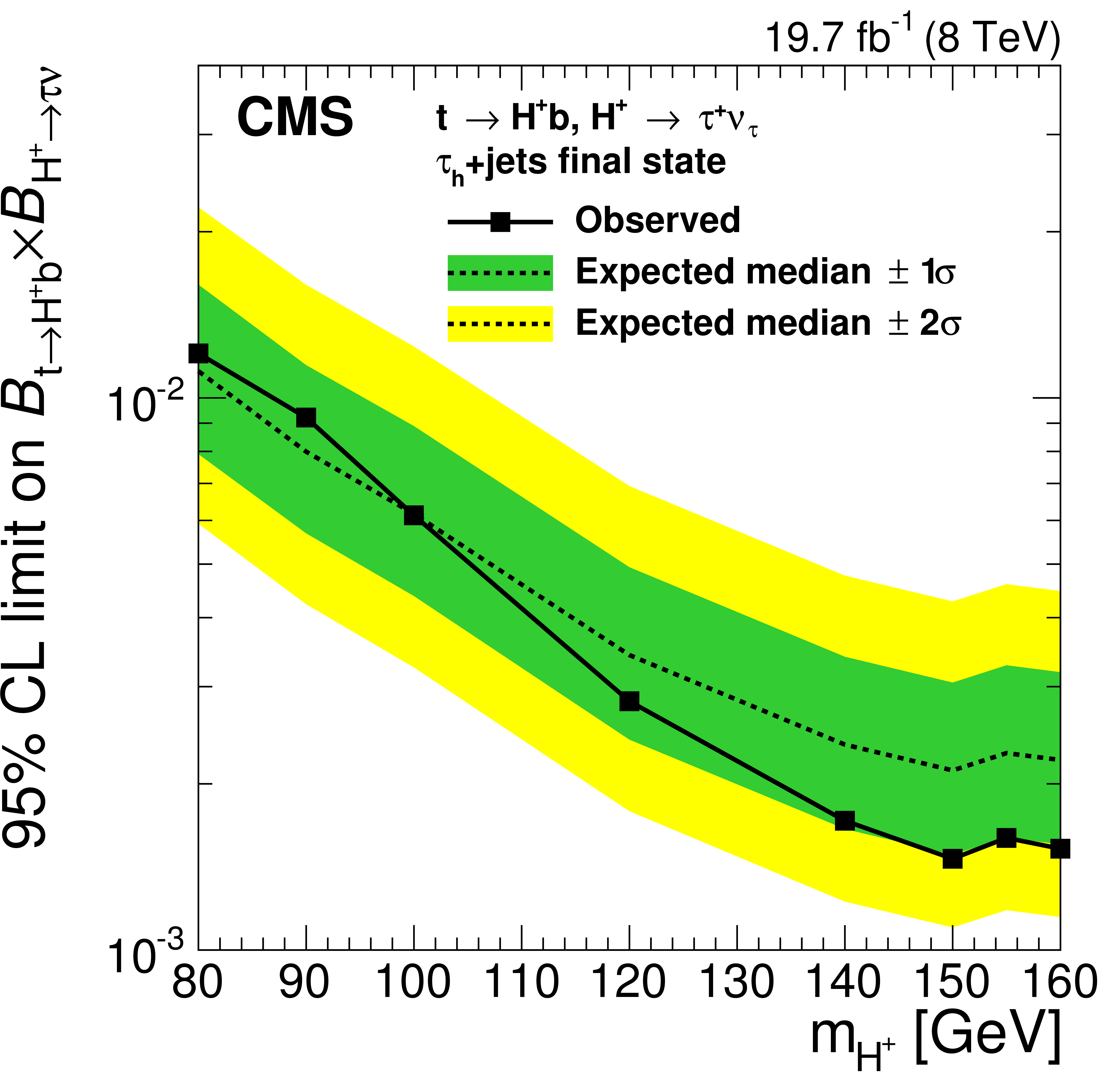
Figure 8-a:
Expected and observed 95% CL model-independent upper limits on (a) $ { {\mathcal {B}( { {\mathrm {t}}\to {\mathrm {H}} ^{+} {\mathrm {b}}} )} \, {\mathcal {B}( { {\mathrm {H}} ^{+}\to {\tau }^{+} {\nu _{\tau }}} )} } $ with $ {m_{ {\mathrm {H}} ^+}} =$ 80-160 GeV, and (b) on $ { {\sigma ({ {\mathrm {p}} {\mathrm {p}}\to {\overline {\mathrm {t}}}( {\mathrm {b}}) {\mathrm {H}} ^{+}})} \, {\mathcal {B}( { {\mathrm {H}} ^{+}\to {\tau }^{+} {\nu _{\tau }}} )} } $ with $ {m_{ {\mathrm {H}} ^+}} =$ 180-600 GeV for the $ { {\mathrm {H}} ^{+}\to {\tau }^{+} {\nu _{\tau }}} $ search in the $ { { {\tau }_{\mathrm {h}}} }$+jets final state. The regions above the solid lines are excluded. |

png pdf |
Figure 8-b:
Expected and observed 95% CL model-independent upper limits on (a) $ { {\mathcal {B}( { {\mathrm {t}}\to {\mathrm {H}} ^{+} {\mathrm {b}}} )} \, {\mathcal {B}( { {\mathrm {H}} ^{+}\to {\tau }^{+} {\nu _{\tau }}} )} } $ with $ {m_{ {\mathrm {H}} ^+}} =$ 80-160 GeV, and (b) on $ { {\sigma ({ {\mathrm {p}} {\mathrm {p}}\to {\overline {\mathrm {t}}}( {\mathrm {b}}) {\mathrm {H}} ^{+}})} \, {\mathcal {B}( { {\mathrm {H}} ^{+}\to {\tau }^{+} {\nu _{\tau }}} )} } $ with $ {m_{ {\mathrm {H}} ^+}} =$ 180-600 GeV for the $ { {\mathrm {H}} ^{+}\to {\tau }^{+} {\nu _{\tau }}} $ search in the $ { { {\tau }_{\mathrm {h}}} }$+jets final state. The regions above the solid lines are excluded. |
png pdf |
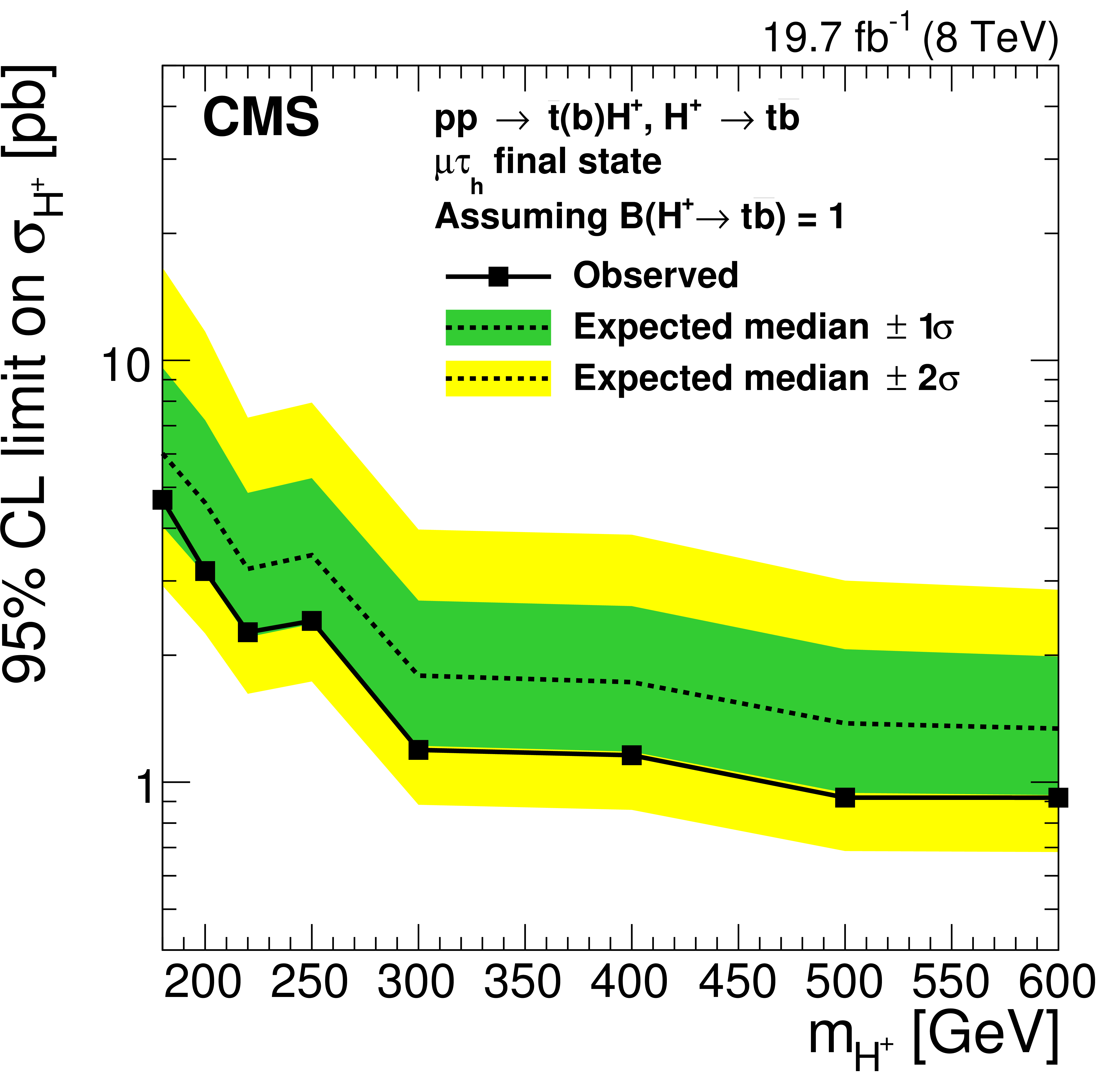
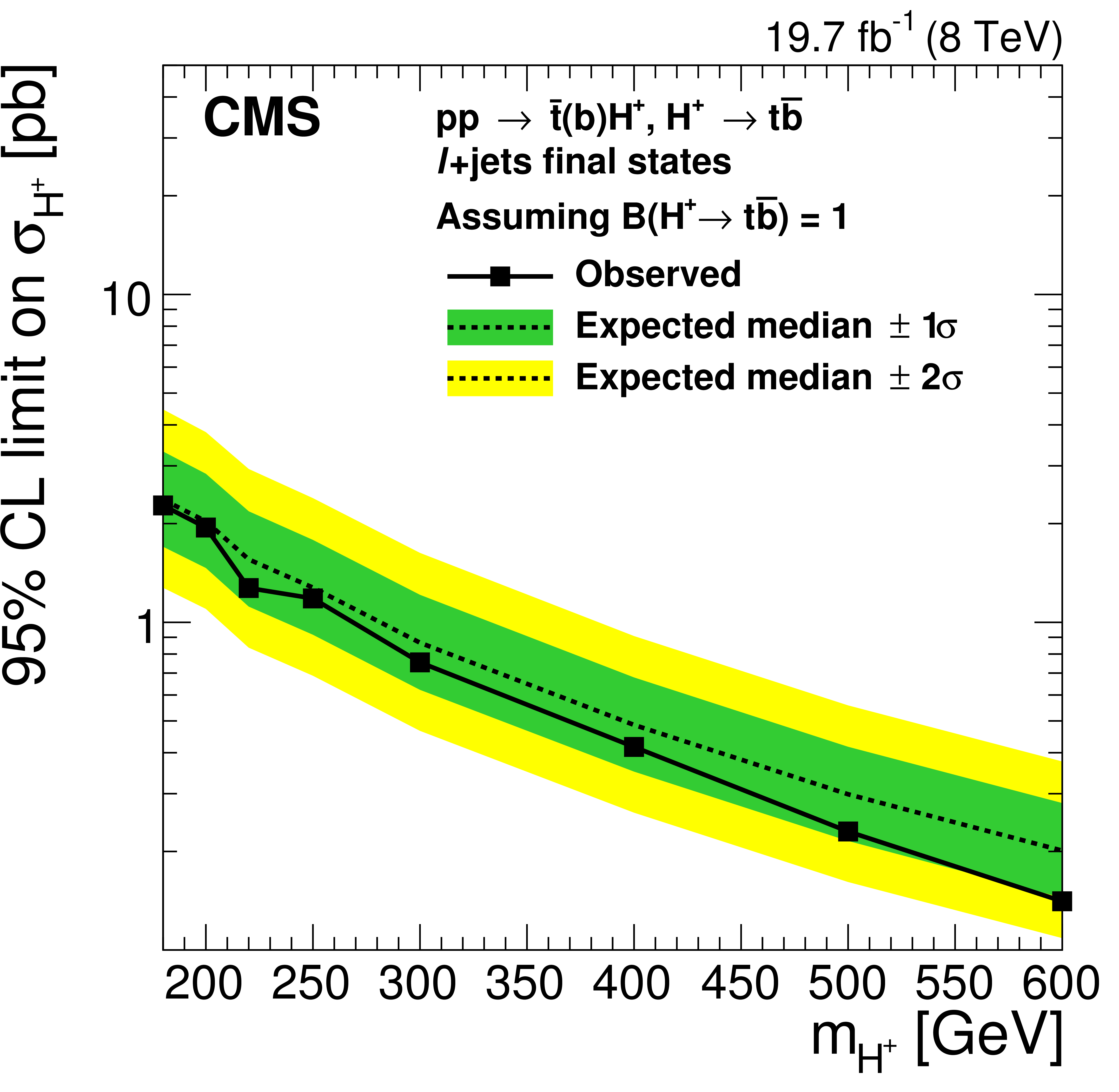
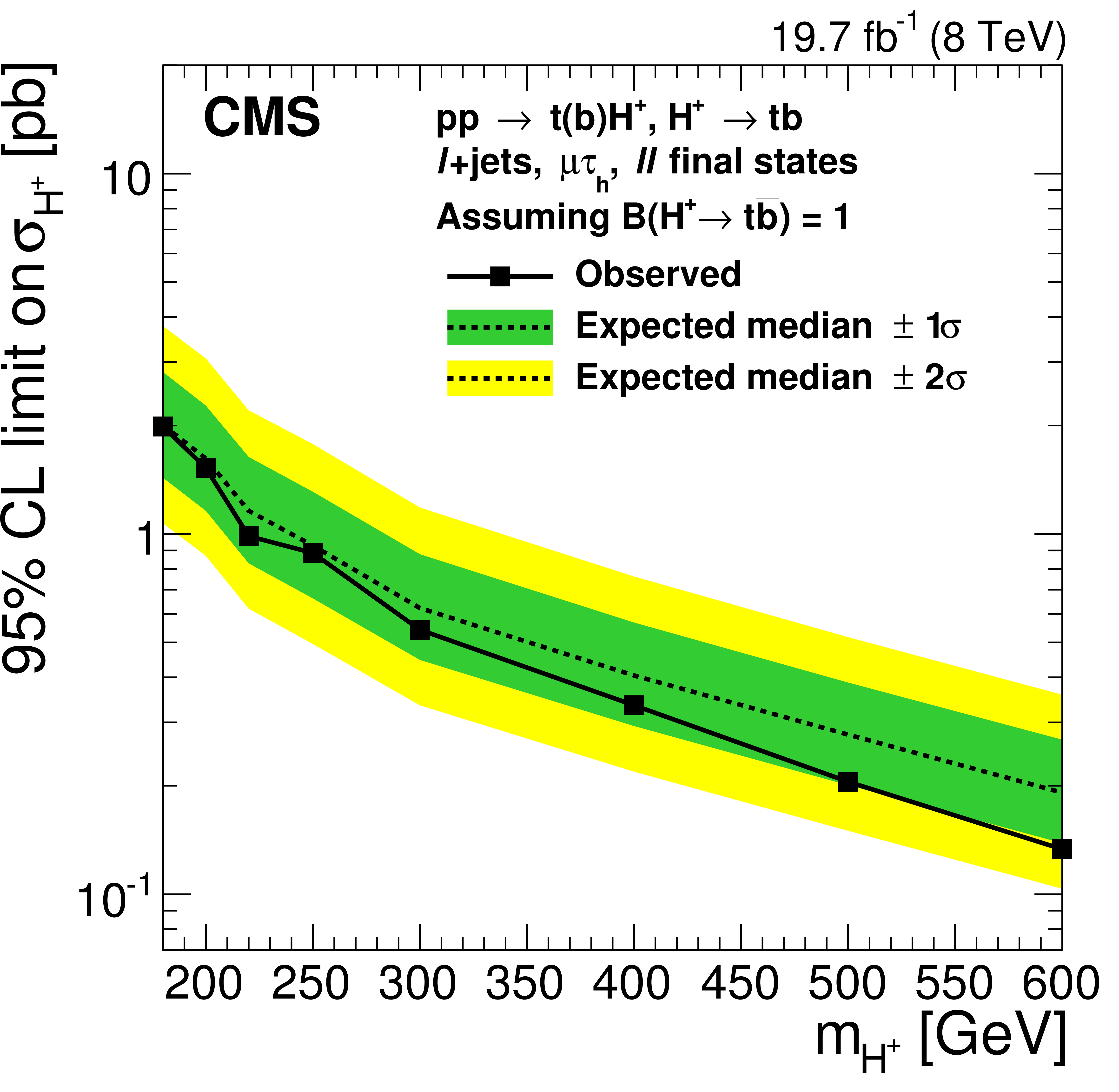
Figure 9-a:
Expected and observed 95% CL upper limits on $ {\sigma ({ {\mathrm {p}} {\mathrm {p}}\to {\overline {\mathrm {t}}}( {\mathrm {b}}) {\mathrm {H}} ^{+}})} $ for the $ { {{\mu }} { {\tau }_{\mathrm {h}}} } $ (a), ${\ell }$+jets (b), and $\ell \ell '$ final states (c) assuming $ {\mathcal {B}( { {\mathrm {H}} ^{+}\to {\mathrm {t}} {\overline {\mathrm {b}}}} )} =$ 1. The regions above the solid lines are excluded. |
png pdf |
Figure 9-b:
Expected and observed 95% CL upper limits on $ {\sigma ({ {\mathrm {p}} {\mathrm {p}}\to {\overline {\mathrm {t}}}( {\mathrm {b}}) {\mathrm {H}} ^{+}})} $ for the $ { {{\mu }} { {\tau }_{\mathrm {h}}} } $ (a), ${\ell }$+jets (b), and $\ell \ell '$ final states (c) assuming $ {\mathcal {B}( { {\mathrm {H}} ^{+}\to {\mathrm {t}} {\overline {\mathrm {b}}}} )} =$ 1. The regions above the solid lines are excluded. |

png pdf |
Figure 9-c:
Expected and observed 95% CL upper limits on $ {\sigma ({ {\mathrm {p}} {\mathrm {p}}\to {\overline {\mathrm {t}}}( {\mathrm {b}}) {\mathrm {H}} ^{+}})} $ for the $ { {{\mu }} { {\tau }_{\mathrm {h}}} } $ (a), ${\ell }$+jets (b), and $\ell \ell '$ final states (c) assuming $ {\mathcal {B}( { {\mathrm {H}} ^{+}\to {\mathrm {t}} {\overline {\mathrm {b}}}} )} =$ 1. The regions above the solid lines are excluded. |
png pdf |
Figure 10:
Expected and observed 95% CL upper limits on $ {\sigma ({ {\mathrm {p}} {\mathrm {p}}\to {\overline {\mathrm {t}}}( {\mathrm {b}}) {\mathrm {H}} ^{+}})} $ for the combination of the $ { {{\mu }} { {\tau }_{\mathrm {h}}} } $, $ {\ell }$+jets, and $\ell \ell '$ final states assuming $ {\mathcal {B}( { {\mathrm {H}} ^{+}\to {\mathrm {t}} {\overline {\mathrm {b}}}} )} =$ 1. The region above the solid line is excluded. |
png pdf |
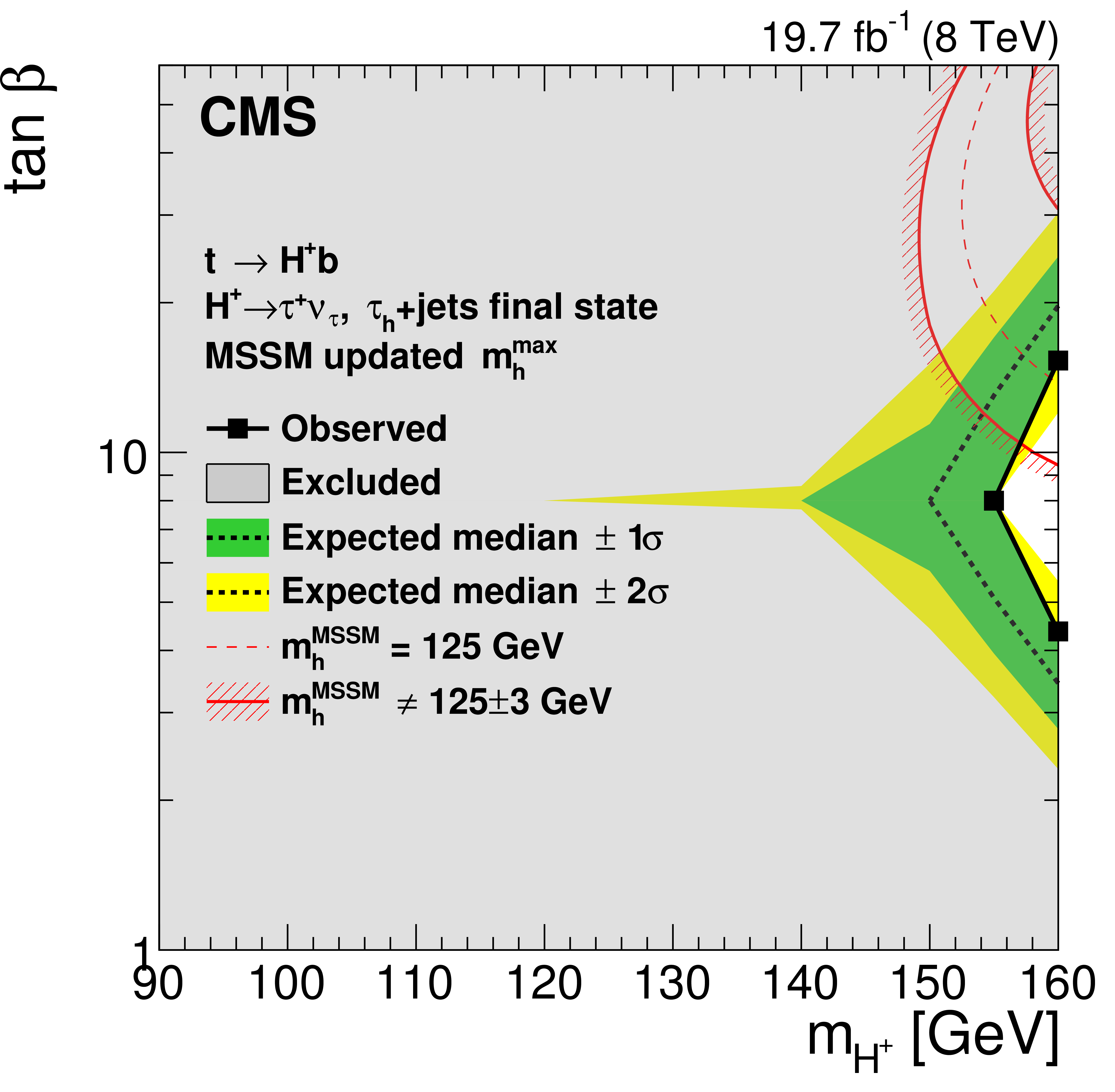
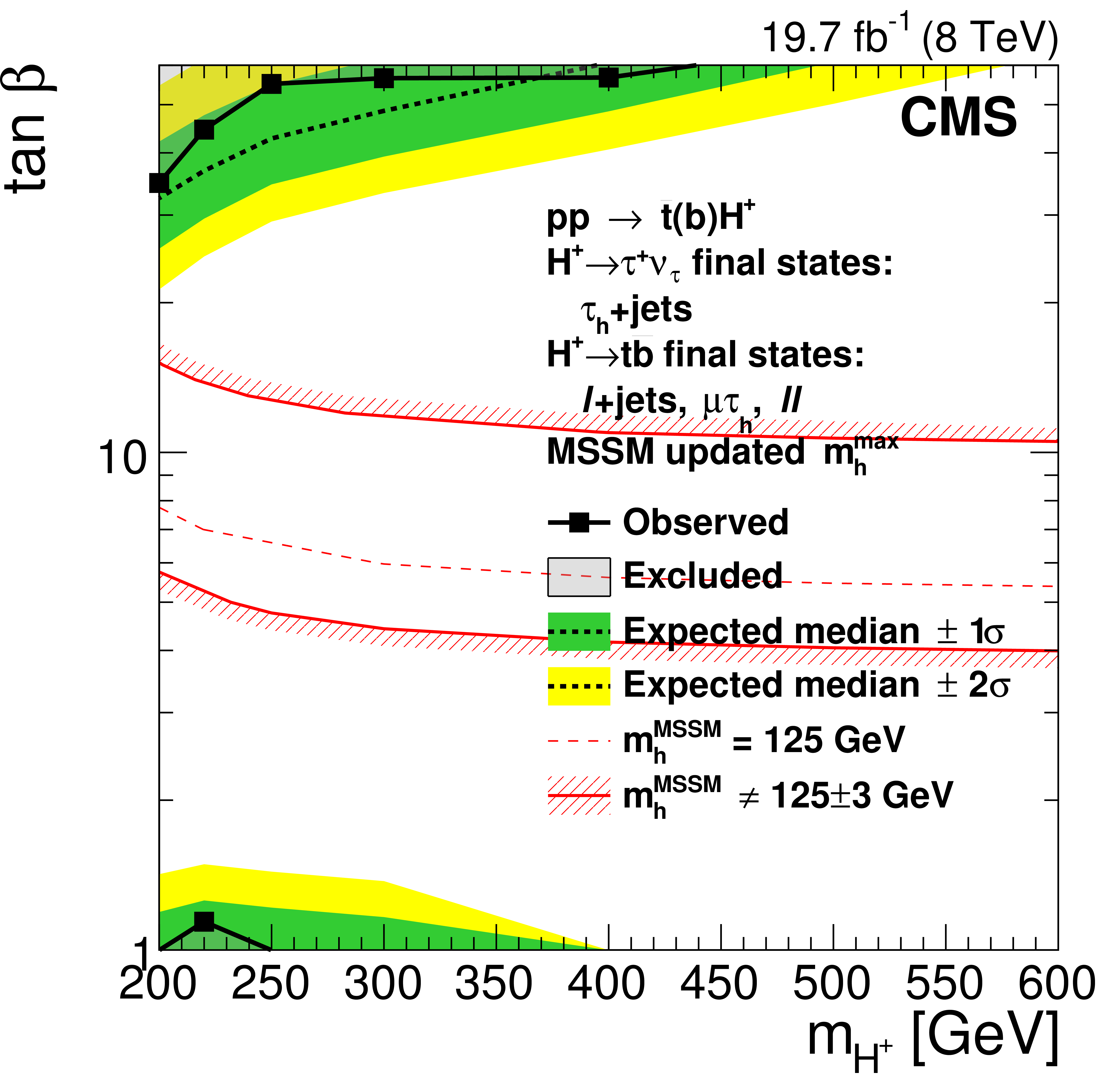
Figure 11-a:
Exclusion region in the MSSM $ {m_{ {\mathrm {H}} ^+}} $-$ { \tan\beta }$ parameter space for (a, c) $ {m_{ {\mathrm {H}} ^+}} = $ 80-160 GeV and for (b, d) $ {m_{ {\mathrm {H}} ^+}} = $ 180-600 GeV in the (a, b) updated MSSM $ {m_\mathrm {h}^\mathrm {max}} $ scenario and (c, d) $ {m_\mathrm {h}^\mathrm {mod-}} $ scenarios [29,33]. In (a) and (c) the limit is derived from the $ { {\mathrm {H}} ^{+}\to {\tau }^{+} {\nu _{\tau }}} $ search with the $ { { {\tau }_{\mathrm {h}}} }$+jets final state, and in (b) and (d) the limit is derived from a combination of all the charged Higgs boson decay modes and final states considered. The $\pm 1 \sigma $ and $\pm 2 \sigma $ bands around the expected limit are also shown. The light-grey region is excluded. The red lines depict the allowed parameter space for the assumption that the discovered scalar boson is the lightest CP-even MSSM Higgs boson with a mass $ {m_{\mathrm {h}}} = 125\pm 3$ GeV, where the uncertainty is the theoretical uncertainty in the Higgs boson mass calculation. |
png pdf |
Figure 11-b:
Exclusion region in the MSSM $ {m_{ {\mathrm {H}} ^+}} $-$ { \tan\beta }$ parameter space for (a, c) $ {m_{ {\mathrm {H}} ^+}} = $ 80-160 GeV and for (b, d) $ {m_{ {\mathrm {H}} ^+}} = $ 180-600 GeV in the (a, b) updated MSSM $ {m_\mathrm {h}^\mathrm {max}} $ scenario and (c, d) $ {m_\mathrm {h}^\mathrm {mod-}} $ scenarios [29,33]. In (a) and (c) the limit is derived from the $ { {\mathrm {H}} ^{+}\to {\tau }^{+} {\nu _{\tau }}} $ search with the $ { { {\tau }_{\mathrm {h}}} }$+jets final state, and in (b) and (d) the limit is derived from a combination of all the charged Higgs boson decay modes and final states considered. The $\pm 1 \sigma $ and $\pm 2 \sigma $ bands around the expected limit are also shown. The light-grey region is excluded. The red lines depict the allowed parameter space for the assumption that the discovered scalar boson is the lightest CP-even MSSM Higgs boson with a mass $ {m_{\mathrm {h}}} = 125\pm 3$ GeV, where the uncertainty is the theoretical uncertainty in the Higgs boson mass calculation. |
png pdf |
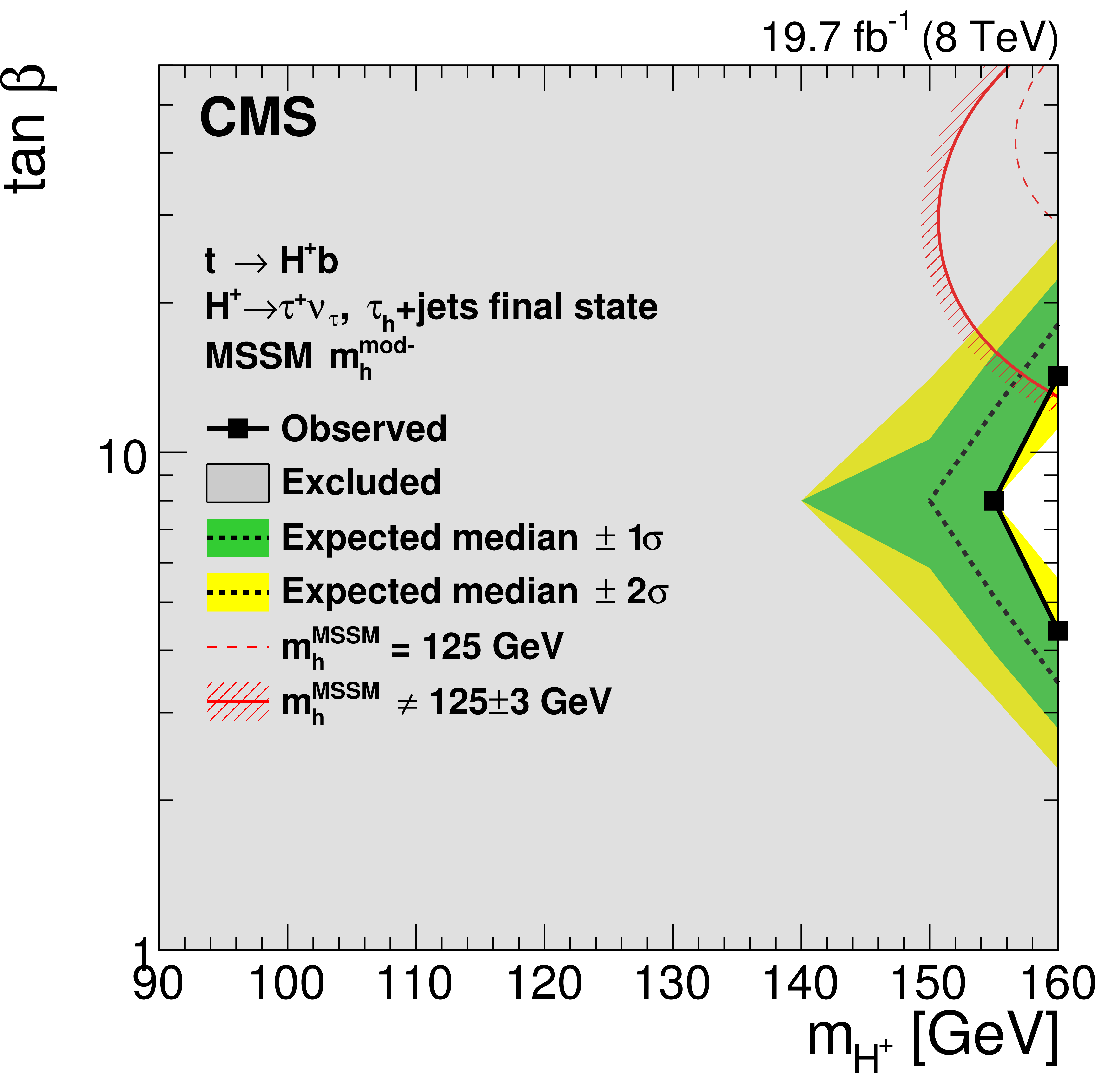
Figure 11-c:
Exclusion region in the MSSM $ {m_{ {\mathrm {H}} ^+}} $-$ { \tan\beta }$ parameter space for (a, c) $ {m_{ {\mathrm {H}} ^+}} = $ 80-160 GeV and for (b, d) $ {m_{ {\mathrm {H}} ^+}} = $ 180-600 GeV in the (a, b) updated MSSM $ {m_\mathrm {h}^\mathrm {max}} $ scenario and (c, d) $ {m_\mathrm {h}^\mathrm {mod-}} $ scenarios [29,33]. In (a) and (c) the limit is derived from the $ { {\mathrm {H}} ^{+}\to {\tau }^{+} {\nu _{\tau }}} $ search with the $ { { {\tau }_{\mathrm {h}}} }$+jets final state, and in (b) and (d) the limit is derived from a combination of all the charged Higgs boson decay modes and final states considered. The $\pm 1 \sigma $ and $\pm 2 \sigma $ bands around the expected limit are also shown. The light-grey region is excluded. The red lines depict the allowed parameter space for the assumption that the discovered scalar boson is the lightest CP-even MSSM Higgs boson with a mass $ {m_{\mathrm {h}}} = 125\pm 3$ GeV, where the uncertainty is the theoretical uncertainty in the Higgs boson mass calculation. |
png pdf |
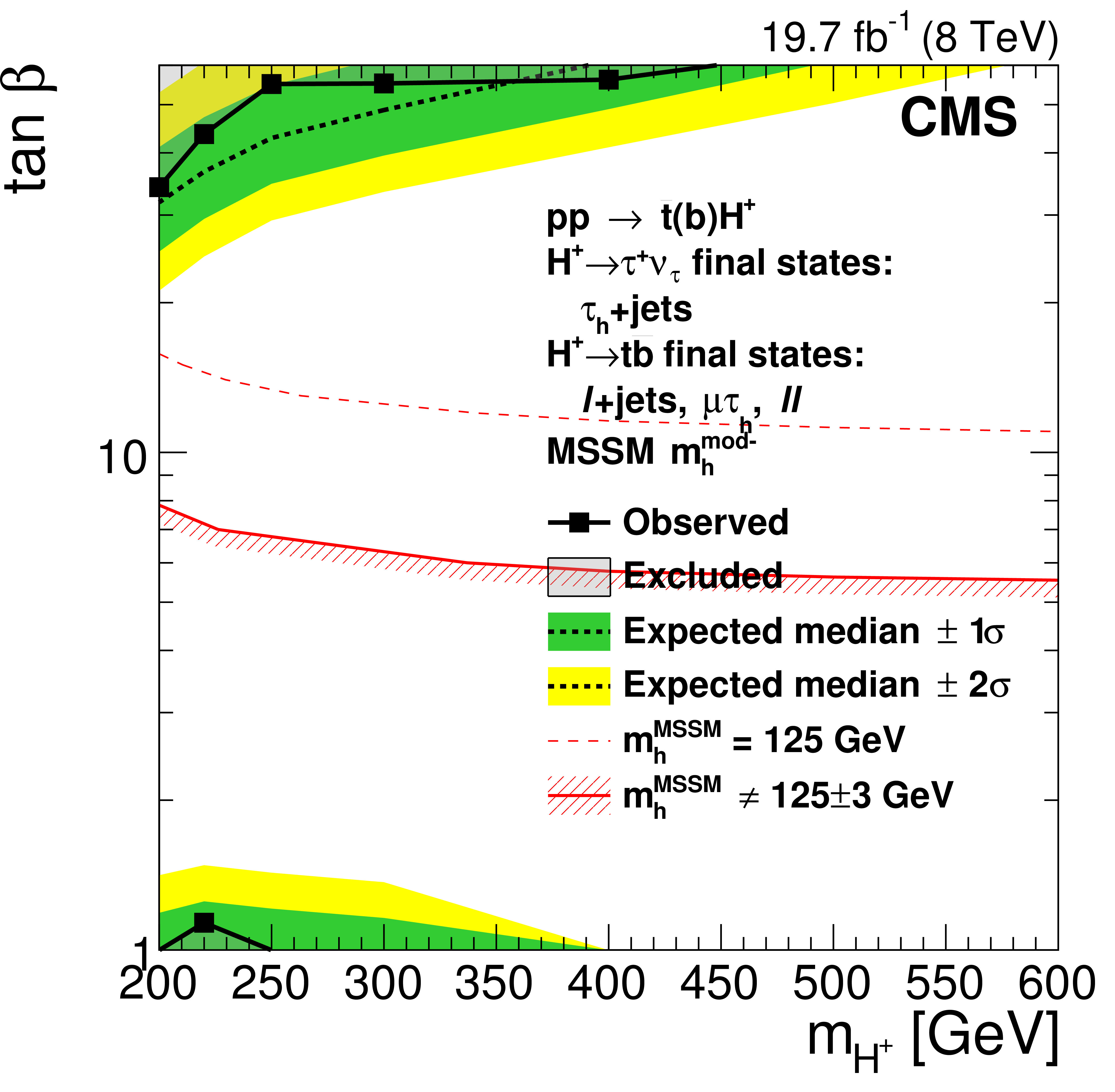
Figure 11-d:
Exclusion region in the MSSM $ {m_{ {\mathrm {H}} ^+}} $-$ { \tan\beta }$ parameter space for (a, c) $ {m_{ {\mathrm {H}} ^+}} = $ 80-160 GeV and for (b, d) $ {m_{ {\mathrm {H}} ^+}} = $ 180-600 GeV in the (a, b) updated MSSM $ {m_\mathrm {h}^\mathrm {max}} $ scenario and (c, d) $ {m_\mathrm {h}^\mathrm {mod-}} $ scenarios [29,33]. In (a) and (c) the limit is derived from the $ { {\mathrm {H}} ^{+}\to {\tau }^{+} {\nu _{\tau }}} $ search with the $ { { {\tau }_{\mathrm {h}}} }$+jets final state, and in (b) and (d) the limit is derived from a combination of all the charged Higgs boson decay modes and final states considered. The $\pm 1 \sigma $ and $\pm 2 \sigma $ bands around the expected limit are also shown. The light-grey region is excluded. The red lines depict the allowed parameter space for the assumption that the discovered scalar boson is the lightest CP-even MSSM Higgs boson with a mass $ {m_{\mathrm {h}}} = 125\pm 3$ GeV, where the uncertainty is the theoretical uncertainty in the Higgs boson mass calculation. |
png pdf |
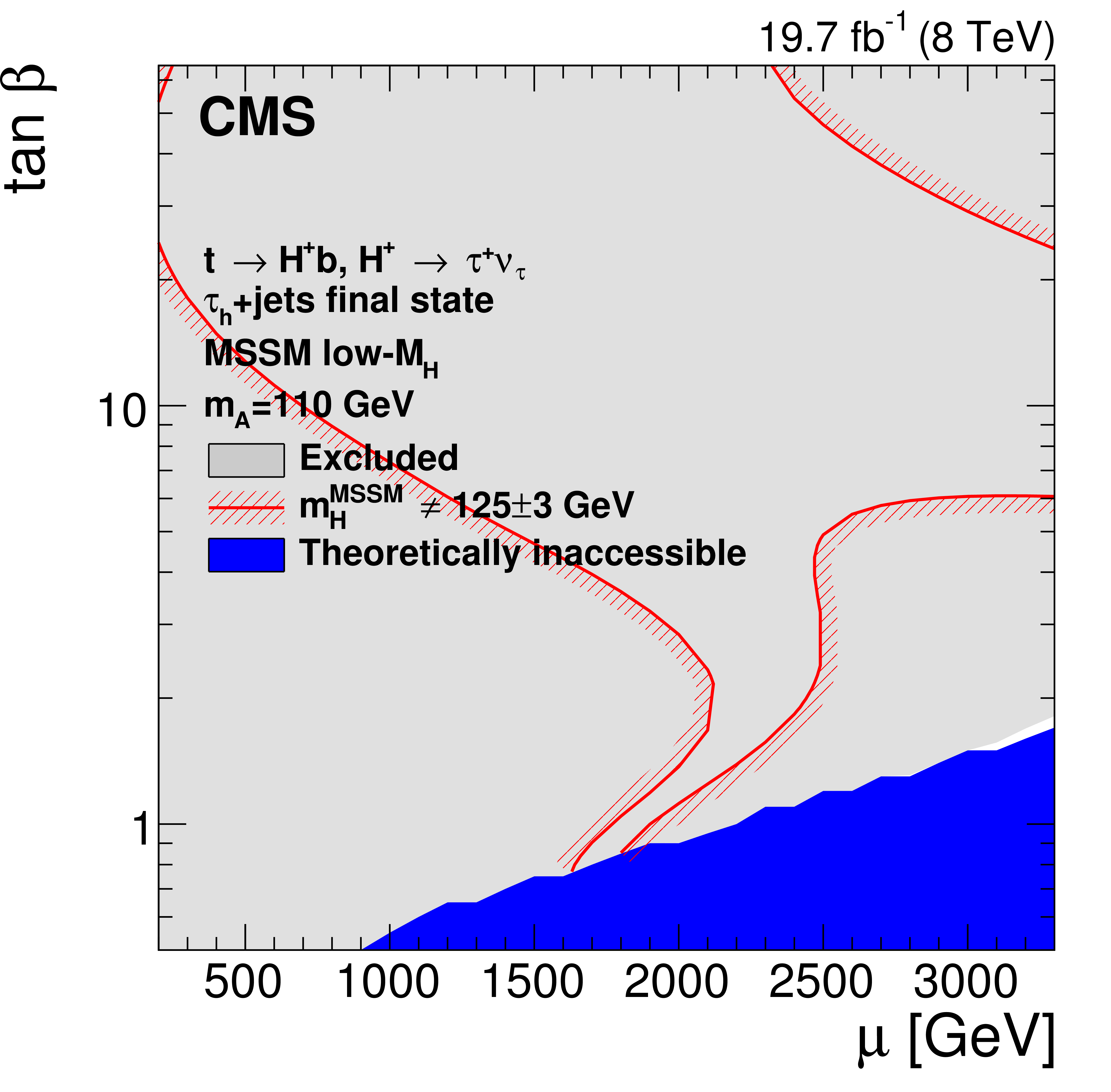
Figure 12:
Exclusion region in the MSSM Higgsino mass parameter ( $ {{\mu }}$) vs. $ { \tan\beta } $ parameter space in the low-$M_ {\mathrm{H}} $ scenario [29,33] with $ {m_{\mathrm {A}}} = $ 110 GeV for the $ { {\mathrm {H}} ^{+}\to {\tau }^{+} {\nu _{\tau }}} $ search with the $ { { {\tau }_{\mathrm {h}}} }$+jets final state. The light-grey region is excluded and the blue region is theoretically inaccessible. The area inside the red lines is the allowed parameter space for the assumption that the discovered scalar boson is the heavy CP-even MSSM Higgs boson with a mass $m_ {\mathrm {H}} =125\pm 3$ GeV, where the uncertainty is the theoretical uncertainty in the Higgs boson mass calculation. |
| Tables | |
png pdf |
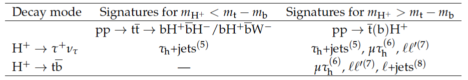
Table 1:
Overview of the charged Higgs boson production processes, decay modes, final states, and mass regions analysed in this paper ($\ell =$ e, $ {{\mu }}$). All final states contain additional jets from the hadronization of b quarks and missing transverse energy from undetected neutrinos. The index after each signature denotes the section where it is discussed. |
png pdf |
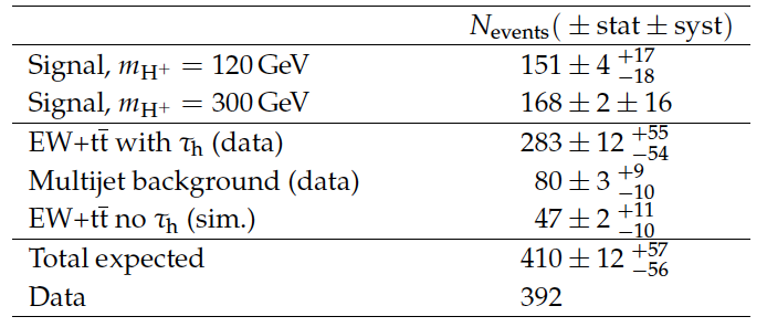
Table 2:
Numbers of expected signal and background events with their statistical and systematic uncertainties listed together with the number of observed events after the full event selection is applied in the $ { { {\tau }_{\mathrm {h}}} }$+jets final state. For illustrative purposes, the expected signal yields are shown for $ {m_{ {\mathrm {H}} ^+}} =$ 120 GeV normalized to $ { {\mathcal {B}( { {\mathrm {t}}\to {\mathrm {H}} ^{+} {\mathrm {b}}} )} \, {\mathcal {B}( { {\mathrm {H}} ^{+}\to {\tau }^{+} {\nu _{\tau }}} )} } = $ 0.01 and for $ {m_{ {\mathrm {H}} ^+}} = $ 300 GeV normalized to $ { {\sigma ({ {\mathrm {p}} {\mathrm {p}}\to {\overline {\mathrm {t}}}( {\mathrm {b}}) {\mathrm {H}} ^{+}})} \, {\mathcal {B}( { {\mathrm {H}} ^{+}\to {\tau }^{+} {\nu _{\tau }}} )} } =$ 1 pb, which are typical values for the sensitivity of this analysis. |

png pdf |
Table 3:
Numbers of expected events in the $ { {{\mu }} { {\tau }_{\mathrm {h}}} } $ final state for the SM backgrounds and in the presence of a signal from $ { {\mathrm {H}} ^{+}\to {\mathrm {t}} {\overline {\mathrm {b}}}} $ and $ { {\mathrm {H}} ^{+}\to {\tau }^{+} {\nu _{\tau }}} $ decays for $ {m_{ {\mathrm {H}} ^+}} =$ 250 GeV are shown together with the number of observed events after the final event selection. For illustrative purposes, the number of signal events is normalized, assuming a 100% branching fraction for each decay mode, to a cross section of 1 pb, which is typical of the cross section sensitivity of this analysis. |
png pdf |
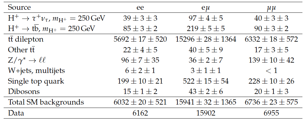
Table 4:
Number of expected events for the SM backgrounds and for signal events with a charged Higgs boson mass of $ {m_{ {\mathrm {H}} ^+}} =$ 250 GeV in the $ {\mathrm {e}} {\mathrm {e}}$, $ {\mathrm {e}} {{\mu }}$, and $ {{\mu }} {{\mu }}$ dilepton final states after the final event selection. For illustrative purposes, the number of signal events is normalized, assuming a 100% branching fraction for each decay mode, to a cross section of 1 pb, which is typical of the cross section sensitivity of this analysis. Event yields are corrected with the trigger and selection efficiencies. Statistical and systematic uncertainties are shown. |
png pdf |
Table 5:
Number of expected events for the SM backgrounds and for signal events with a charged Higgs boson mass of $ {m_{ {\mathrm {H}} ^+}} =$ 250 GeV in the $ {\ell }$+jets final states after the final event selection. Normalizations for W+light-flavour jets, Wc, Wb, and $ {\mathrm {t}\overline {\mathrm {t}}} $ are derived from data. Normalizations for other backgrounds are based on simulation. For illustrative purposes, the signal is normalized, assuming $ {\mathcal {B}( { {\mathrm {t}}\to {\mathrm {H}} ^{+} {\mathrm {b}}} )} =$ 1, to a cross section of 1 pb, which is typical of the cross section sensitivity of this analysis. Statistical and systematic uncertainties are shown. |
png pdf |
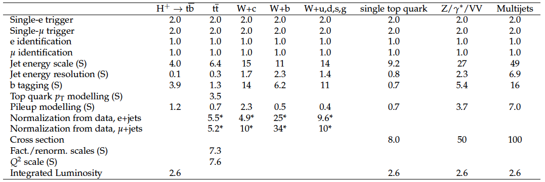
Table 6:
The systematic uncertainties on event yields (in %) for the charged Higgs boson signal processes $ {\mathrm {t}\overline {\mathrm {t}}} \to {\mathrm {b}} {\mathrm {H}} ^+ {\overline {\mathrm {b}}} {\mathrm {H}} ^-$ ($ {\mathrm {H}} ^+ {\mathrm {H}} ^-$), $ {\mathrm {t}\overline {\mathrm {t}}} \to {\mathrm {b}} {\mathrm {H}} ^+ {\overline {\mathrm {b}}} {\mathrm {W}}^-$ ($ {\mathrm {H}} ^+ {\mathrm {W}}^-$), and $ {\mathrm {p}} {\mathrm {p}}\to {\overline {\mathrm {t}}}( {\mathrm {b}}) {\mathrm {H}} ^{+}$ ($ {\mathrm {H}} ^+$) and for the background processes. The uncertainties which depend on the $ {m_\mathrm {T}} $ distribution bin are marked with (S) and for these the maximum integrated value of the negative or positive variation is displayed. Empty cells indicate that an uncertainty does not affect the sample. The uncertainty values within the rows are considered to be fully correlated and the values within the columns are considered to be uncorrelated. A minus sign in front of an uncertainty value means anticorrelation with other values in the same row. |
png pdf |
Table 7:
The systematic uncertainties for the $ { {{\mu }} { {\tau }_{\mathrm {h}}} } $ final state (in %) for backgrounds, and for signal events from $ { {\mathrm {H}} ^{+}\to {\mathrm {t}} {\overline {\mathrm {b}}}} $ decays for $ {m_{ {\mathrm {H}} ^+}} =$ 250 GeV. These systematic uncertainties are given as the input to the exclusion limit calculation. The uncertainties that depend on the b-tagged jets multiplicity distribution bin are marked with (S) and for these the maximum integrated value of the negative or positive variation is displayed. Empty cells indicate that an uncertainty does not affect the sample. The uncertainty values within the rows are considered to be fully correlated and the values within the columns are considered to be uncorrelated. The uncertainties in the cross sections are to be considered uncorrelated for different samples and fully correlated for different final states of the same sample (e.g. the different $ {\mathrm {t}\overline {\mathrm {t}}} $ decays). |
png pdf |
Table 8:
The systematic uncertainties (in %) for backgrounds, and for signal events from $ { {\mathrm {H}} ^{+}\to {\mathrm {t}} {\overline {\mathrm {b}}}} $ decays for the dilepton channels for a charged Higgs boson mass $ {m_{ {\mathrm {H}} ^+}} =$ 250 GeV. The $ {\mathrm {e}} {{\mu }}$ final state is shown as a representative example. These systematic uncertainties are given as the input to the exclusion limit calculation. The uncertainties that depend on the b-tagged jets multiplicity distribution bin are marked with (S) and for these the maximum integrated value of the negative or positive variation is displayed. Empty cells indicate that an uncertainty does not affect the sample. The uncertainty values within the rows are considered to be fully correlated and the values within the columns are considered to be uncorrelated. The uncertainties in the cross sections are to be considered uncorrelated for different samples and fully correlated for different final states of the same sample (e.g. the different $ {\mathrm {t}\overline {\mathrm {t}}} $ decay channels). |
png pdf |
Table 9:
The systematic uncertainties (in %) for backgrounds, and for signal events from $ { {\mathrm {H}} ^{+}\to {\mathrm {t}} {\overline {\mathrm {b}}}} $ decays for the $\ell $+jets channels for a charged Higgs boson mass $ {m_{ {\mathrm {H}} ^+}} =$ 250 GeV. The uncertainties that depend on the shape of the ${H_{\mathrm {T}}} $ distribution bin are marked with (S) and for these the maximum integrated value of the negative or positive variation is displayed. Empty cells indicate that an uncertainty does not affect the sample. The uncertainty values within the rows are considered to be fully correlated, with the exception of cross section and data-driven normalization, which are considered to be uncorrelated. The uncertainty values within the columns are considered to be uncorrelated. Uncertainties labelled with a "*" are only present in the CR with an implicit unconstrained parameter correlated across all bins (Sec. 8.2). The values for these are assigned prior to the setting of limits. |
png pdf |
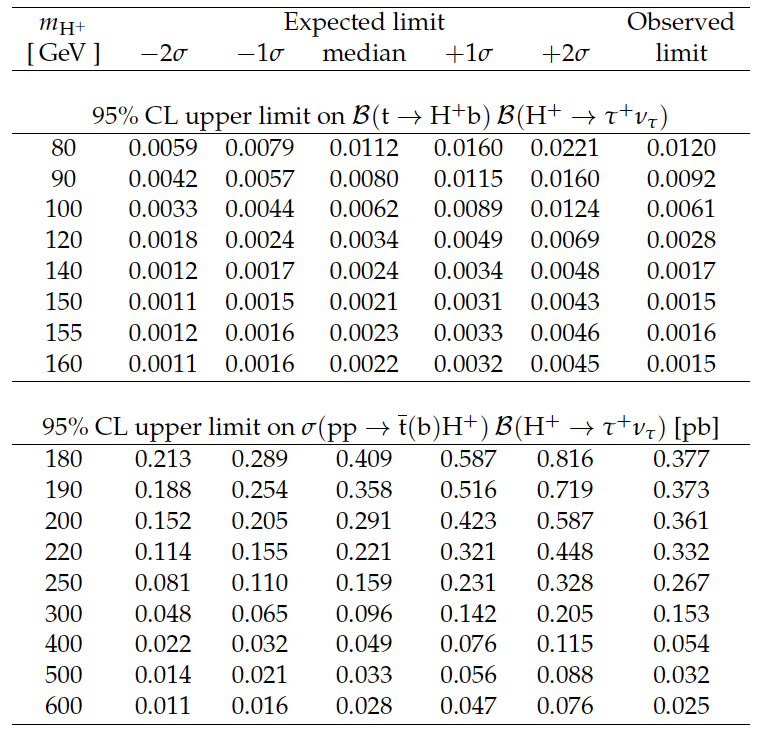
Table 10:
Expected and observed 95% CL model-independent upper limits on $ { {\mathcal {B}( { {\mathrm {t}}\to {\mathrm {H}} ^{+} {\mathrm {b}}} )} \, {\mathcal {B}( { {\mathrm {H}} ^{+}\to {\tau }^{+} {\nu _{\tau }}} )} } $ for $ {m_{ {\mathrm {H}} ^+}} =$ 80-160 GeV (top), and on $ { {\sigma ({ {\mathrm {p}} {\mathrm {p}}\to {\overline {\mathrm {t}}}( {\mathrm {b}}) {\mathrm {H}} ^{+}})} \, {\mathcal {B}( { {\mathrm {H}} ^{+}\to {\tau }^{+} {\nu _{\tau }}} )} } $ for $ {m_{ {\mathrm {H}} ^+}} = $ 180-600 GeV (bottom), for the $ { {\mathrm {H}} ^{+}\to {\tau }^{+} {\nu _{\tau }}} $ search in the $ { { {\tau }_{\mathrm {h}}} }$+jets final state. |
png pdf |
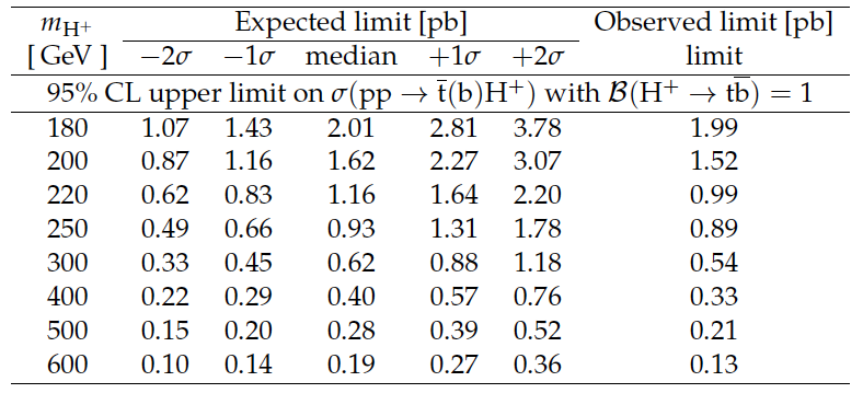
Table 11:
Expected and observed 95% CL upper limits on $ { {\sigma ({ {\mathrm {p}} {\mathrm {p}}\to {\overline {\mathrm {t}}}( {\mathrm {b}}) {\mathrm {H}} ^{+}})} \, {\mathcal {B}( { {\mathrm {H}} ^{+}\to {\mathrm {t}} {\overline {\mathrm {b}}}} )} } $ assuming $ {\mathcal {B}( { {\mathrm {H}} ^{+}\to {\mathrm {t}} {\overline {\mathrm {b}}}} )} = $ 1 for the combination of the $ { {{\mu }} { {\tau }_{\mathrm {h}}} } $, $ {\ell }$+jets, and $\ell \ell '$ final states. |
| Summary |
|
A search is performed for a charged Higgs boson with the CMS detector using a data sample corresponding to an integrated luminosity of 19.7 $\pm$ 0.5 fb$^{-1}$ in proton-proton collisions at $\sqrt{s} =$ 8 TeV. The charged Higgs boson production in $ \mathrm{ t \bar{t} } $ decays and in $ \mathrm{ pp \to t (b)H^+ }$ is studied assuming $\mathrm{ H^+ \to \tau^+ \nu_{\tau} } $ and $ \mathrm{ H^+ to t \bar{b} }$ decay modes, using the $\tau_{\mathrm{h}}$+jets, $\mu tau_{\mathrm{h}}$, $\ell$+jets, and $\ell\ell$' final states. Data are found to agree with the SM expectations. Model-independent limits without an assumption on the charged Higgs boson branching fractions are derived for the $\mathrm{ H^+ \to \tau^+ \nu_{\tau} } $ decay mode in the $\tau_{\mathrm{h}}$+jets final state. Upper limits at 95% CL of $\mathcal{B}( \mathrm{ t \to H^+ b })\, \mathcal{B}( \mathrm{ H^+ \to \tau^+ \nu_{\tau} } ) =$ 1.2-0.15% and $ \sigma ( \mathrm{ pp \to \bar{t} (b) H^+ } )\, \mathcal{B}( \mathrm{ H^+ \to \tau^+ \nu_{\tau} } ) =$ 0.38-0.025 pb are set for charged Higgs boson mass ranges $ m_{\mathrm{H}^+} =$ 80-160 GeV and $ m_{\mathrm{H}^+} =$ 180-600 GeV, respectively. Assuming $ \mathcal{B}( \mathrm{H^+ \to t \bar{b} } ) = $ 1, a 95% CL upper limit of $ \sigma( \mathrm{ pp \to \bar{t} (b) H^+ }) =$ 2.0-0.13 pb is set for a combination of the $\mu \tau_{\mathrm{h}} $, $\ell$+jets, and $\ell \ell$' final states for $m_{\mathrm{H}^+} =$ 180-600 GeV. This is the first experimental result on the $\mathrm{ H^+ \to t \bar{b} }$ decay mode. Here, cross section $ \sigma( \mathrm{ pp \to t (b) H^{\pm} } ) $ stands for the sum $ \sigma( \mathrm{ pp \to \bar{t} (b)H^{+} } ) + \sigma( \mathrm{ pp \to t(\bar{b})H^{-} } ) $. The results are interpreted in different MSSM benchmark scenarios and used to set exclusion limits in the $m_{\mathrm{H}^+}$-$\tan\beta$ parameter spaces. In the various models, a lower bound on the charged Higgs boson mass of about 155 GeV is set assuming $ m_{\mathrm{h}} = 125 \pm 3$ GeV. The light-stop scenario is excluded for $m_{\mathrm{H}^+} <$ 160 GeV assuming $ m_{\mathrm{h}} = 125 \pm 3$ GeV, and the low-$M_{\mathrm{H}}$ scenario defined in Refs. [29, 33] is completely excluded assuming $ m_{\mathrm{h}} = 125 \pm 3$ GeV. |
|
|
Compact Muon Solenoid LHC, CERN |
|

|

|

|

|

|