

Compact Muon Solenoid
LHC, CERN
| CMS-SUS-11-022 ; CERN-PH-EP-2012-290 | ||
| Search for supersymmetry in final states with missing transverse energy and 0, 1, 2, or at least 3 b-quark jets in 7 TeV pp collisions using the variable $\alpha_T$ | ||
| CMS Collaboration | ||
| 30 October 2012 | ||
| J. High Energy Phys. 01 (2013) 077 | ||
| Abstract: A search for supersymmetry in final states with jets and missing transverse energy is performed in pp collisions at a centre-of-mass energy of $sqrt{s}$ = 7 TeV. The data sample corresponds to an integrated luminosity of 4.98 inverse femtobarns collected by the CMS experiment at the LHC. In this search, a dimensionless kinematic variable, alphaT, is used as the main discriminator between events with genuine and misreconstructed missing transverse energy. The search is performed in a signal region that is binned in the scalar sum of the transverse energy of jets and the number of jets identified as originating from a bottom quark. No excess of events over the standard model expectation is found. Exclusion limits are set in the parameter space of the constrained minimal supersymmetric extension of the standard model, and also in simplified models, with a special emphasis on compressed spectra and third-generation scenarios. | ||
| Links: e-print arXiv:1210.8115 [hep-ex] (PDF) ; CDS record ; inSPIRE record ; Public twiki page ; CADI line (restricted) ; | ||
| Figures | |
png pdf |
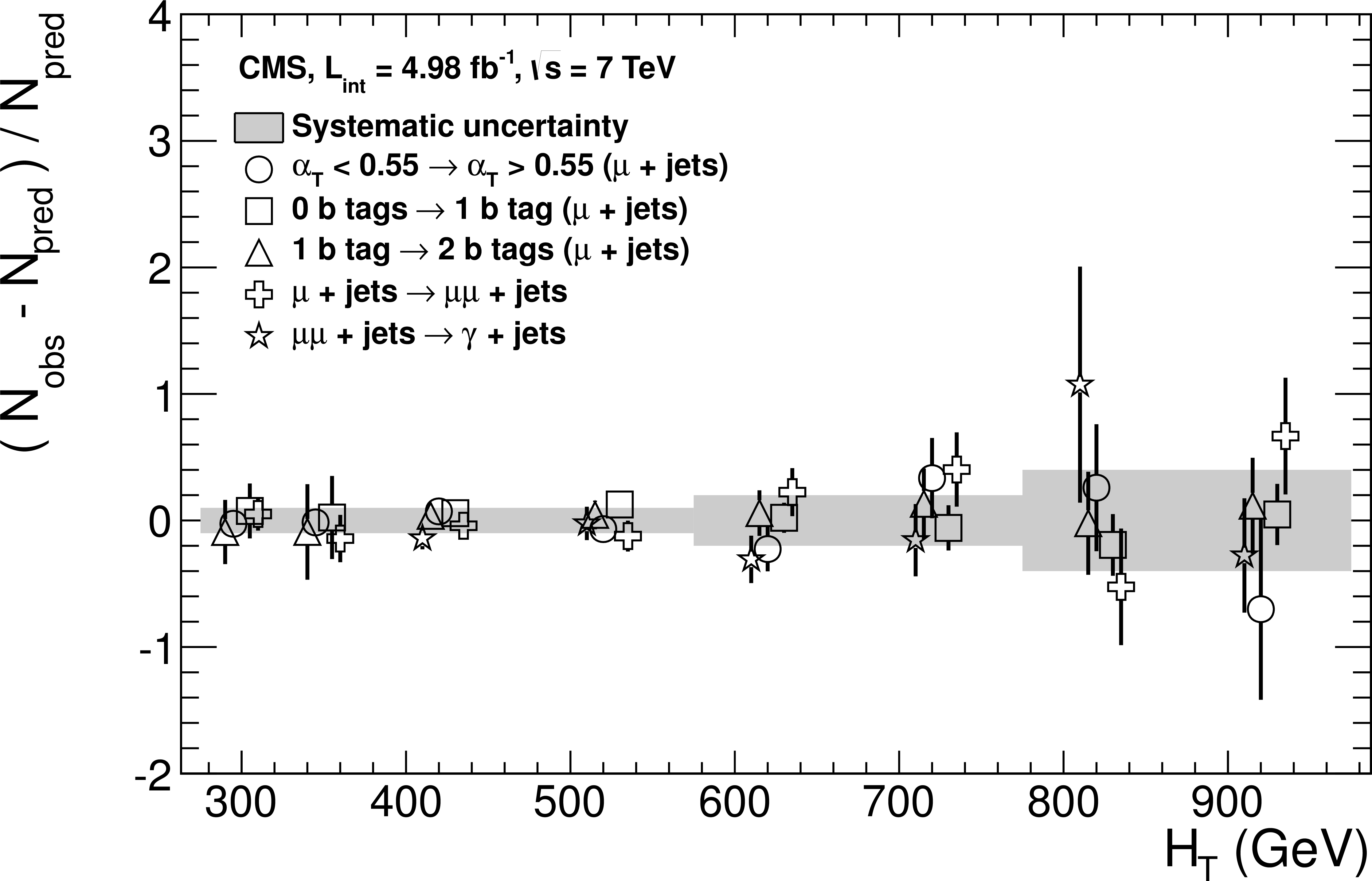
Figure 1:
A set of five closure tests, described in the text, that use the three data control samples to probe key ingredients of the simulation modelling of the SM backgrounds, as a function of $H_\mathrm {T}$. Error bars represent statistical uncertainties only. The shaded bands represent the $H_\mathrm {T}$-dependent systematic uncertainties assigned to the transfer factors. |

png pdf |
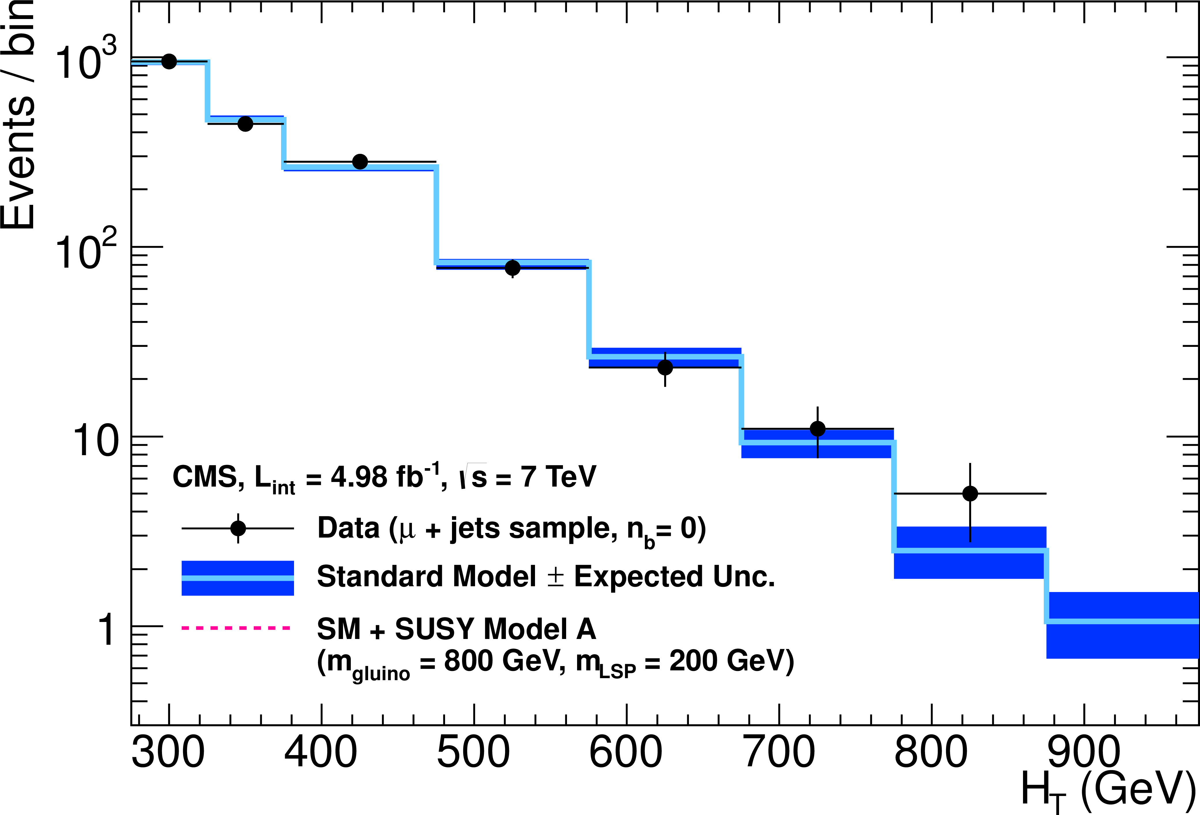
Figure 2-a:
Comparison of the observed yields and SM expectations given by the simultaneous fit in bins of $H_\mathrm {T}$ for the (a) signal region, (b) $ {\mu } $+ jets, (c) $ {\mu \mu } $ + jets, and (d) $ {\gamma } $ + jets samples when requiring exactly zero reconstructed b-quark jets. The observed event yields in data (black dots) and the expectations and their uncertainties, as determined by the simultaneous fit, for all SM processes (light blue solid line with dark blue bands) are shown. For illustrative purposes only, the signal expectation (magenta dashed line) in the signal region for the simplified model $A$ (defined in Section 7.2) with $m_{ \tilde{g} } =$ 800 GeV and $m_\mathrm {LSP} =$ 200 GeV is superimposed on the SM background expectation. |
png pdf |
Figure 2-b:
Comparison of the observed yields and SM expectations given by the simultaneous fit in bins of $H_\mathrm {T}$ for the (a) signal region, (b) $ {\mu } $+ jets, (c) $ {\mu \mu } $ + jets, and (d) $ {\gamma } $ + jets samples when requiring exactly zero reconstructed b-quark jets. The observed event yields in data (black dots) and the expectations and their uncertainties, as determined by the simultaneous fit, for all SM processes (light blue solid line with dark blue bands) are shown. For illustrative purposes only, the signal expectation (magenta dashed line) in the signal region for the simplified model $A$ (defined in Section 7.2) with $m_{ \tilde{g} } =$ 800 GeV and $m_\mathrm {LSP} =$ 200 GeV is superimposed on the SM background expectation. |
png pdf |
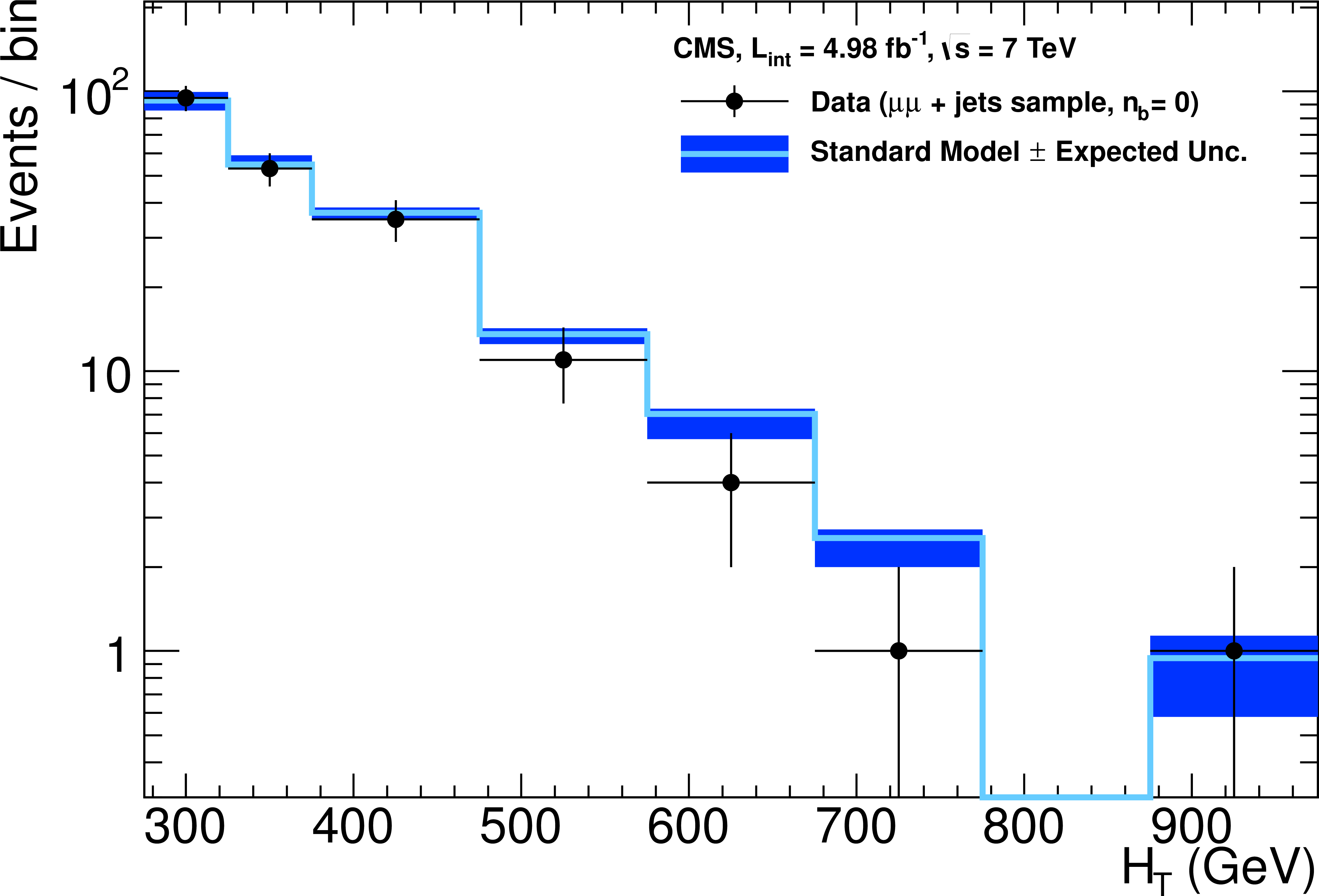
Figure 2-c:
Comparison of the observed yields and SM expectations given by the simultaneous fit in bins of $H_\mathrm {T}$ for the (a) signal region, (b) $ {\mu } $+ jets, (c) $ {\mu \mu } $ + jets, and (d) $ {\gamma } $ + jets samples when requiring exactly zero reconstructed b-quark jets. The observed event yields in data (black dots) and the expectations and their uncertainties, as determined by the simultaneous fit, for all SM processes (light blue solid line with dark blue bands) are shown. For illustrative purposes only, the signal expectation (magenta dashed line) in the signal region for the simplified model $A$ (defined in Section 7.2) with $m_{ \tilde{g} } =$ 800 GeV and $m_\mathrm {LSP} =$ 200 GeV is superimposed on the SM background expectation. |
png pdf |
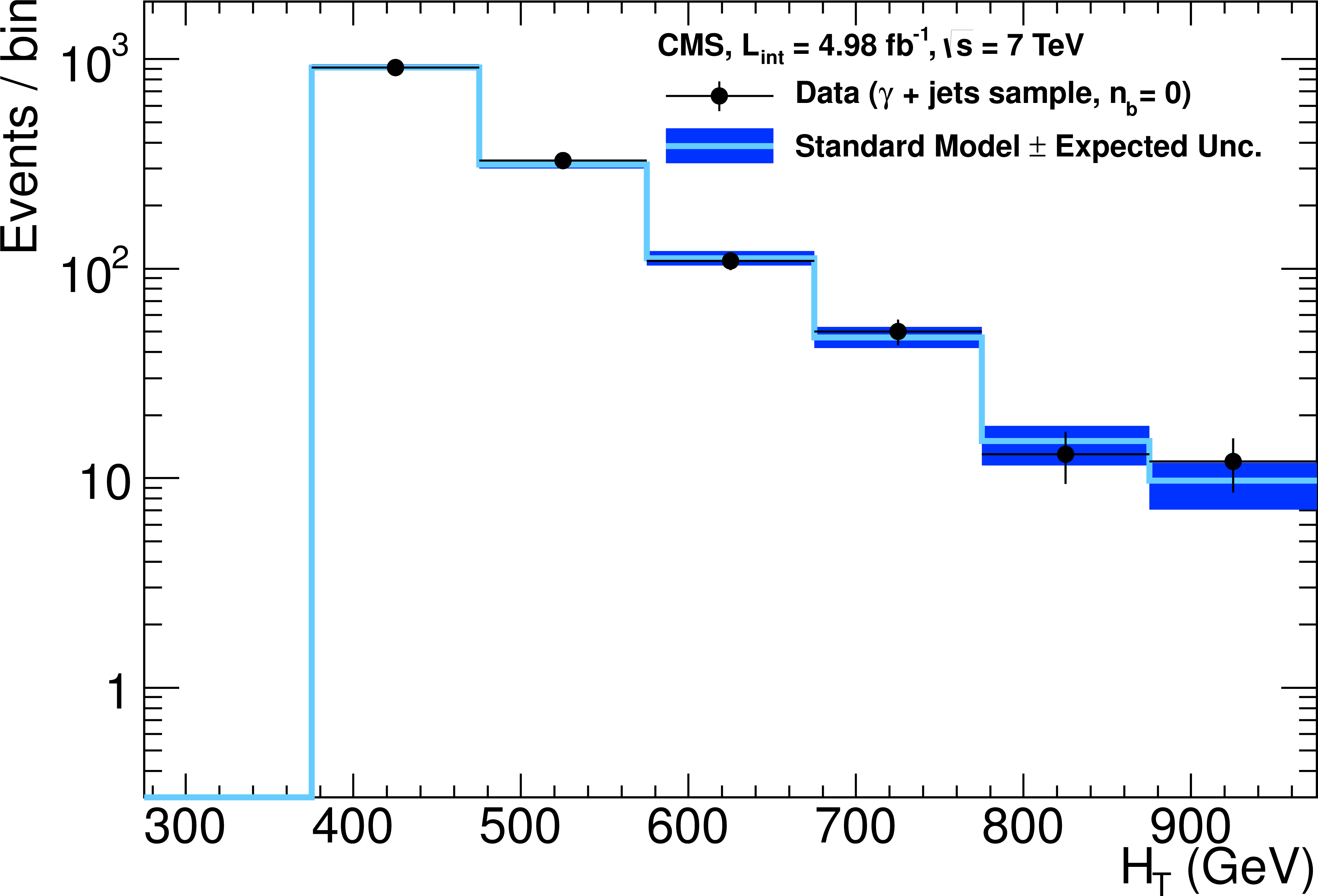
Figure 2-d:
Comparison of the observed yields and SM expectations given by the simultaneous fit in bins of $H_\mathrm {T}$ for the (a) signal region, (b) $ {\mu } $+ jets, (c) $ {\mu \mu } $ + jets, and (d) $ {\gamma } $ + jets samples when requiring exactly zero reconstructed b-quark jets. The observed event yields in data (black dots) and the expectations and their uncertainties, as determined by the simultaneous fit, for all SM processes (light blue solid line with dark blue bands) are shown. For illustrative purposes only, the signal expectation (magenta dashed line) in the signal region for the simplified model $A$ (defined in Section 7.2) with $m_{ \tilde{g} } =$ 800 GeV and $m_\mathrm {LSP} =$ 200 GeV is superimposed on the SM background expectation. |
png pdf |
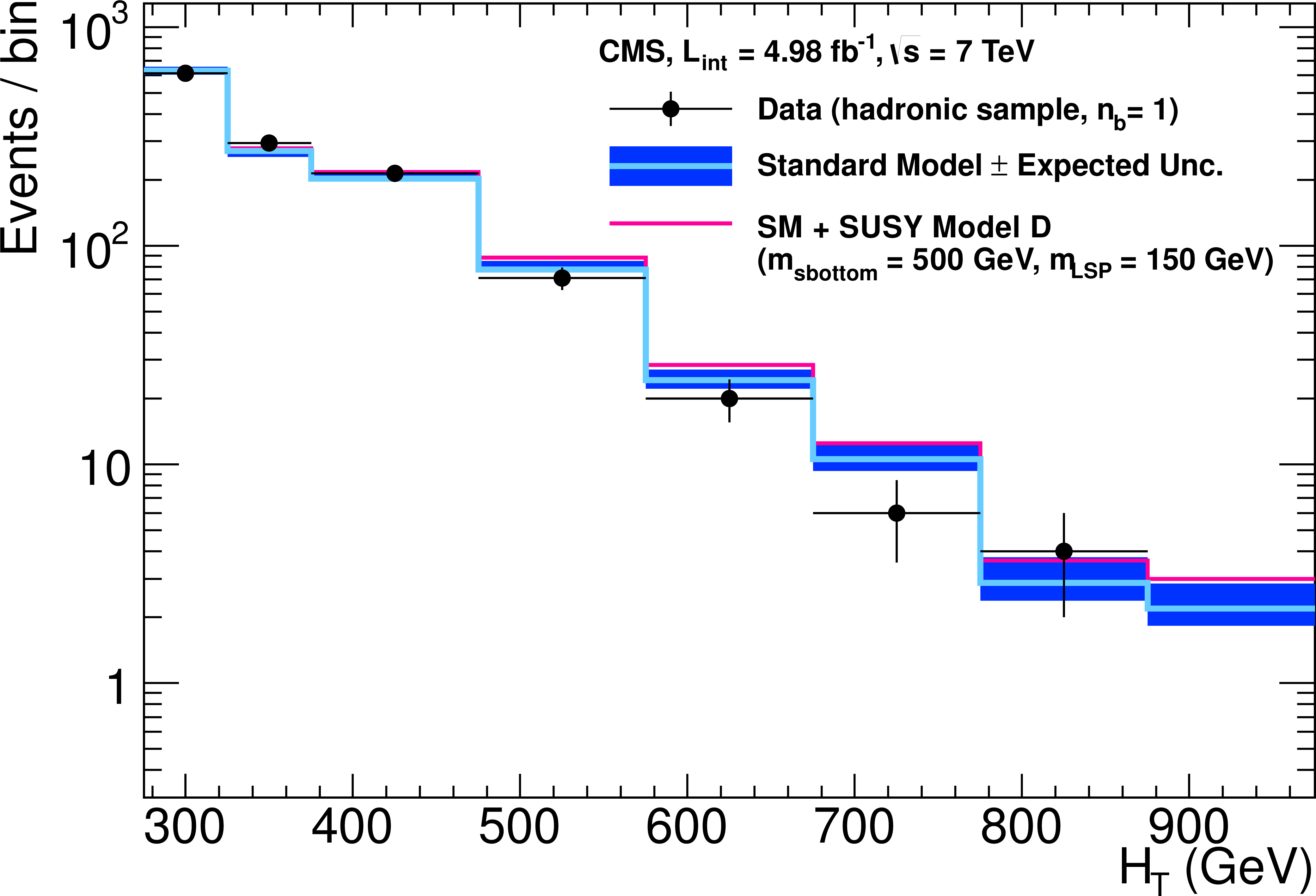
Figure 3-a:
Comparison of the observed yields and SM expectations given by the simultaneous fit in bins of $H_\mathrm {T}$ for the (a) signal region, (b) $ {\mu }$ + jets, (c) $ {\mu \mu }$ + jets, and (d) $ {\gamma }$ + jets samples. Same as Fig. 2, except requiring exactly one reconstructed b-quark jet. The observed event yields in data (black dots) and the expectations and their uncertainties, as determined by the simultaneous fit, for all SM processes (light blue solid line with dark blue bands) are shown. For illustrative purposes only, the signal expectation (magenta solid line) in the signal region for the simplified model $D$ (defined in Section 7.2) with $m_{ \tilde{g} } =$ 500 GeV and $m_\mathrm {LSP} = $150 GeV is superimposed on the SM background expectation. |
png pdf |
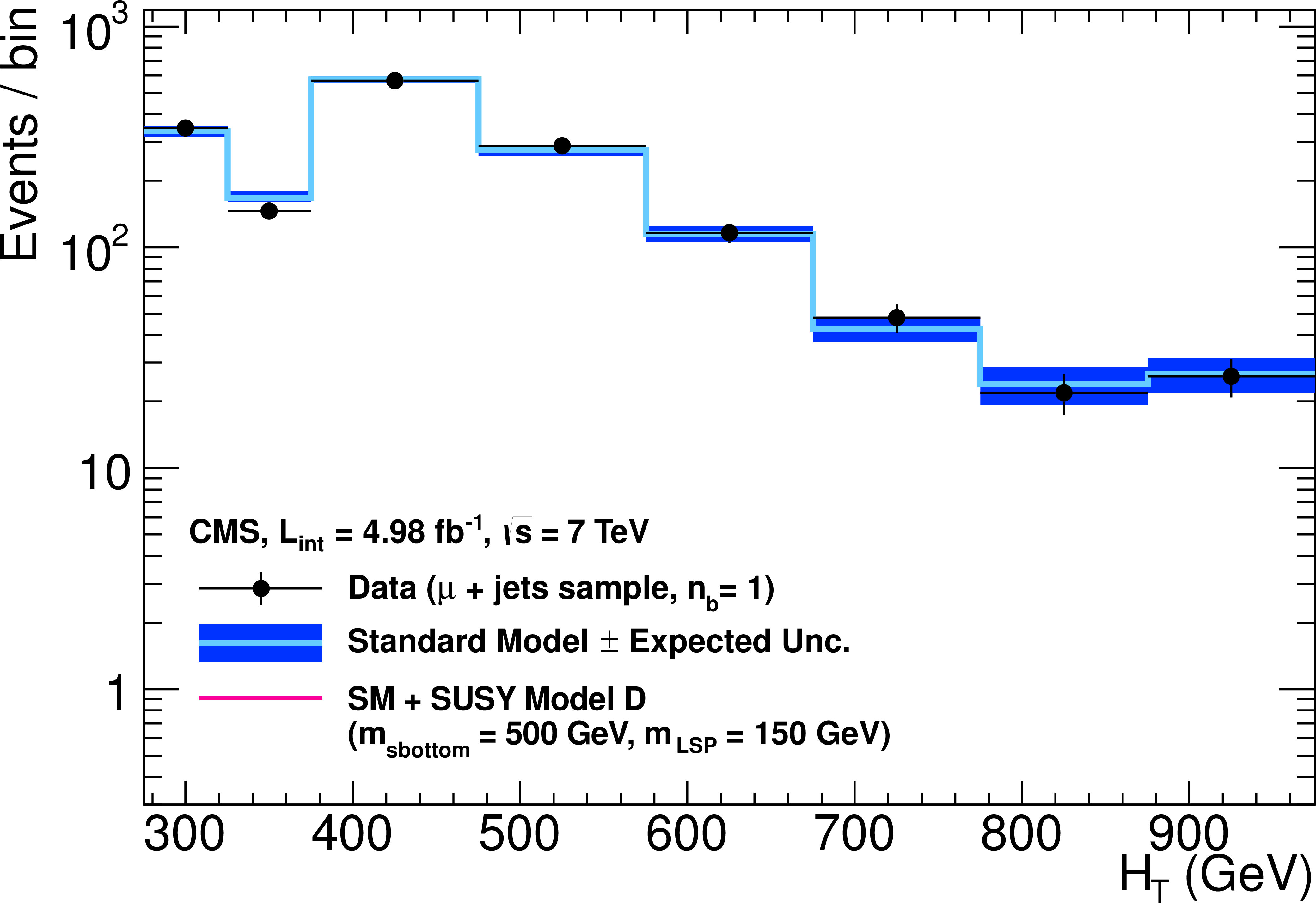
Figure 3-b:
Comparison of the observed yields and SM expectations given by the simultaneous fit in bins of $H_\mathrm {T}$ for the (a) signal region, (b) $ {\mu }$ + jets, (c) $ {\mu \mu }$ + jets, and (d) $ {\gamma }$ + jets samples. Same as Fig. 2, except requiring exactly one reconstructed b-quark jet. The observed event yields in data (black dots) and the expectations and their uncertainties, as determined by the simultaneous fit, for all SM processes (light blue solid line with dark blue bands) are shown. For illustrative purposes only, the signal expectation (magenta solid line) in the signal region for the simplified model $D$ (defined in Section 7.2) with $m_{ \tilde{g} } =$ 500 GeV and $m_\mathrm {LSP} = $150 GeV is superimposed on the SM background expectation. |

png pdf |
Figure 3-c:
Comparison of the observed yields and SM expectations given by the simultaneous fit in bins of $H_\mathrm {T}$ for the (a) signal region, (b) $ {\mu }$ + jets, (c) $ {\mu \mu }$ + jets, and (d) $ {\gamma }$ + jets samples. Same as Fig. 2, except requiring exactly one reconstructed b-quark jet. The observed event yields in data (black dots) and the expectations and their uncertainties, as determined by the simultaneous fit, for all SM processes (light blue solid line with dark blue bands) are shown. For illustrative purposes only, the signal expectation (magenta solid line) in the signal region for the simplified model $D$ (defined in Section 7.2) with $m_{ \tilde{g} } =$ 500 GeV and $m_\mathrm {LSP} = $150 GeV is superimposed on the SM background expectation. |
png pdf |
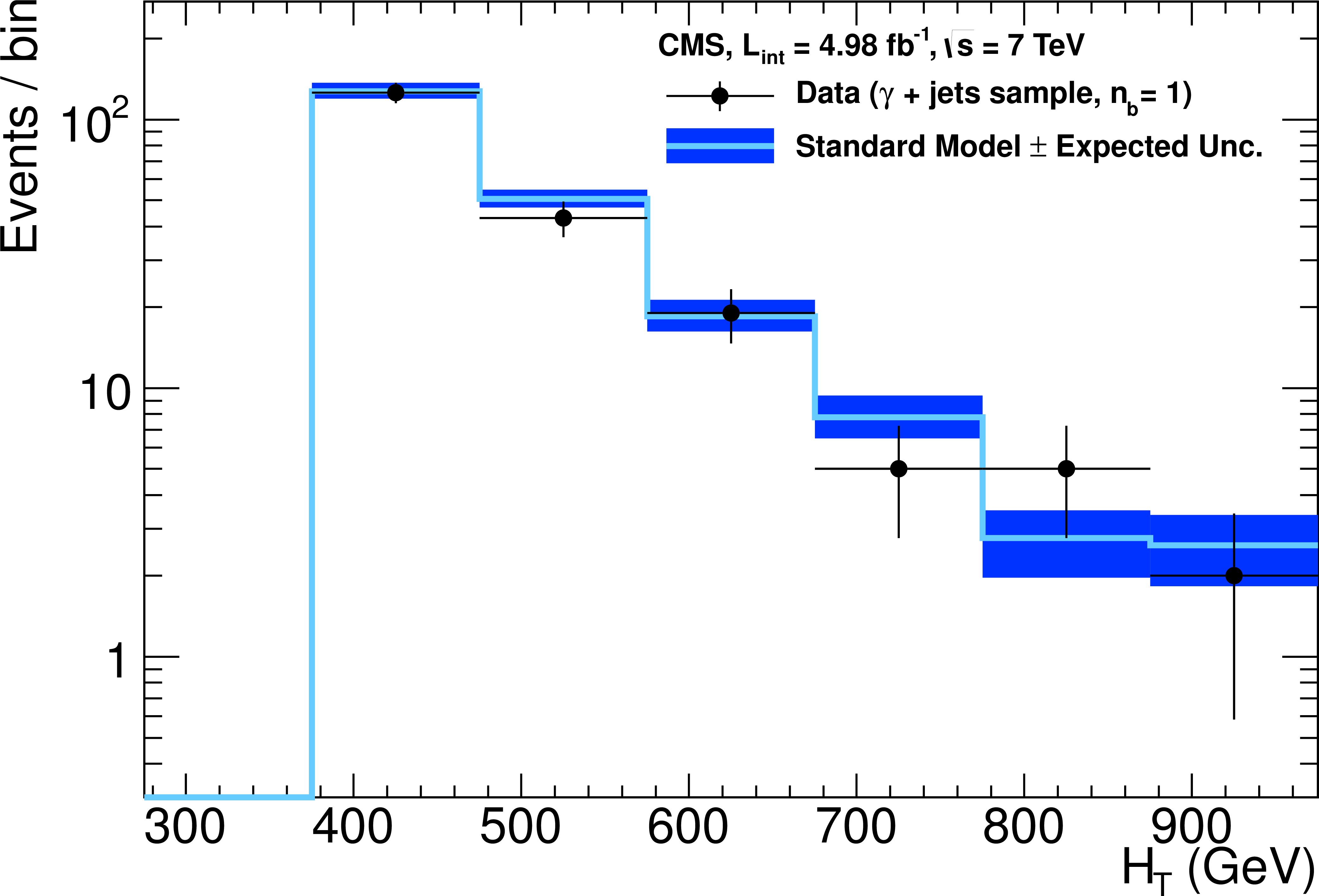
Figure 3-d:
Comparison of the observed yields and SM expectations given by the simultaneous fit in bins of $H_\mathrm {T}$ for the (a) signal region, (b) $ {\mu }$ + jets, (c) $ {\mu \mu }$ + jets, and (d) $ {\gamma }$ + jets samples. Same as Fig. 2, except requiring exactly one reconstructed b-quark jet. The observed event yields in data (black dots) and the expectations and their uncertainties, as determined by the simultaneous fit, for all SM processes (light blue solid line with dark blue bands) are shown. For illustrative purposes only, the signal expectation (magenta solid line) in the signal region for the simplified model $D$ (defined in Section 7.2) with $m_{ \tilde{g} } =$ 500 GeV and $m_\mathrm {LSP} = $150 GeV is superimposed on the SM background expectation. |

png pdf |
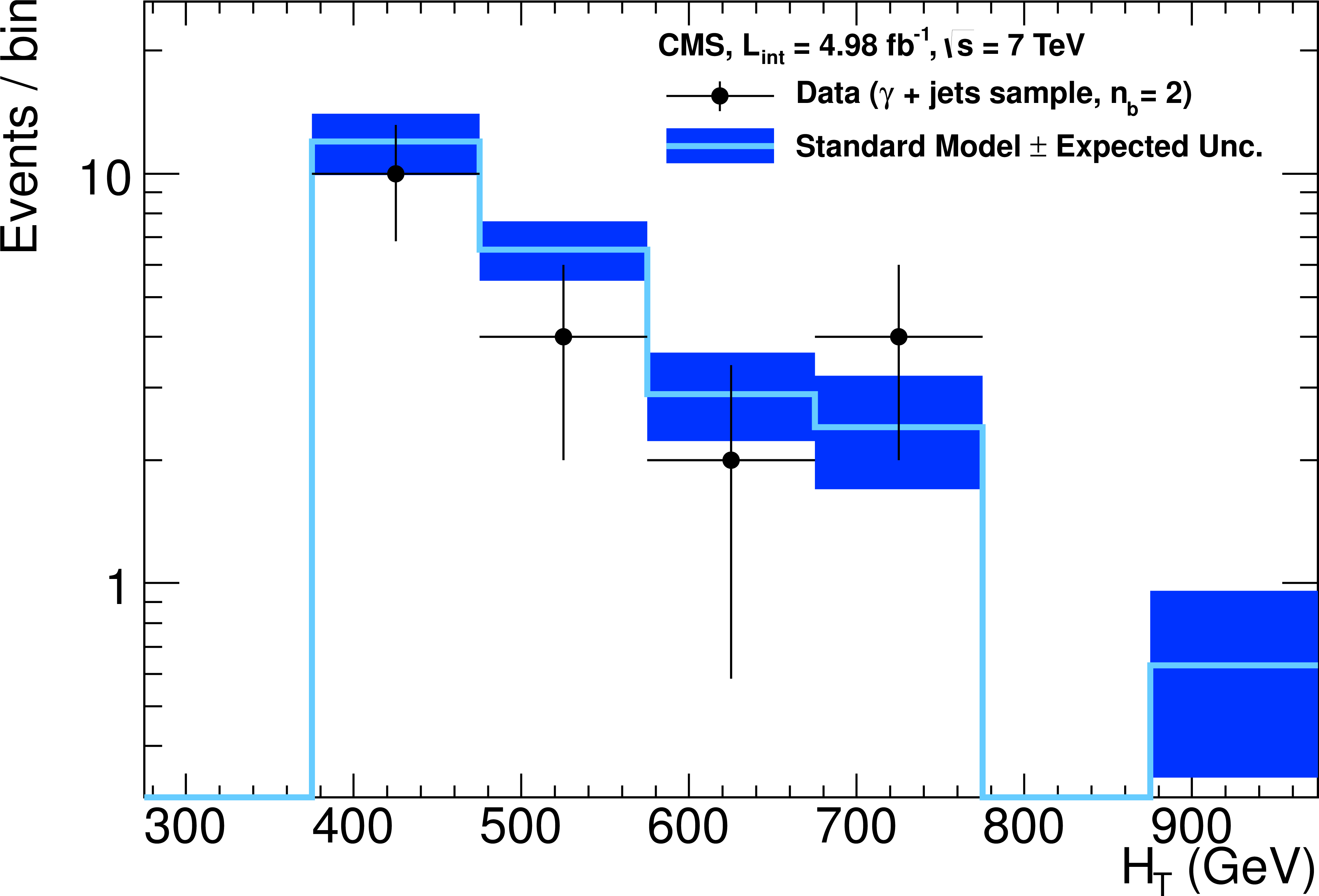
Figure 4-a:
Comparison of the observed yields and SM expectations given by the simultaneous fit in bins of $H_\mathrm {T}$ for the (a) signal region, (b) $ {\mu }$ + jets, (c) $ {\mu \mu } $ + jets, and (d) $ {\gamma } $ + jets samples. Same as Fig. 2, except requiring exactly two reconstructed b-quark jets. The observed event yields in data (black dots) and the expectations and their uncertainties, as determined by the simultaneous fit, for all SM processes (light blue solid line with dark blue bands) are shown. For illustrative purposes only, the signal expectation (magenta solid line) in the signal region for the simplified model $D$ (defined in Section 7.2) with $m_{ \tilde{g} } =$ 500 GeV and $m_\mathrm {LSP} =$ 150 GeV is superimposed on the SM background expectation. |
png pdf |
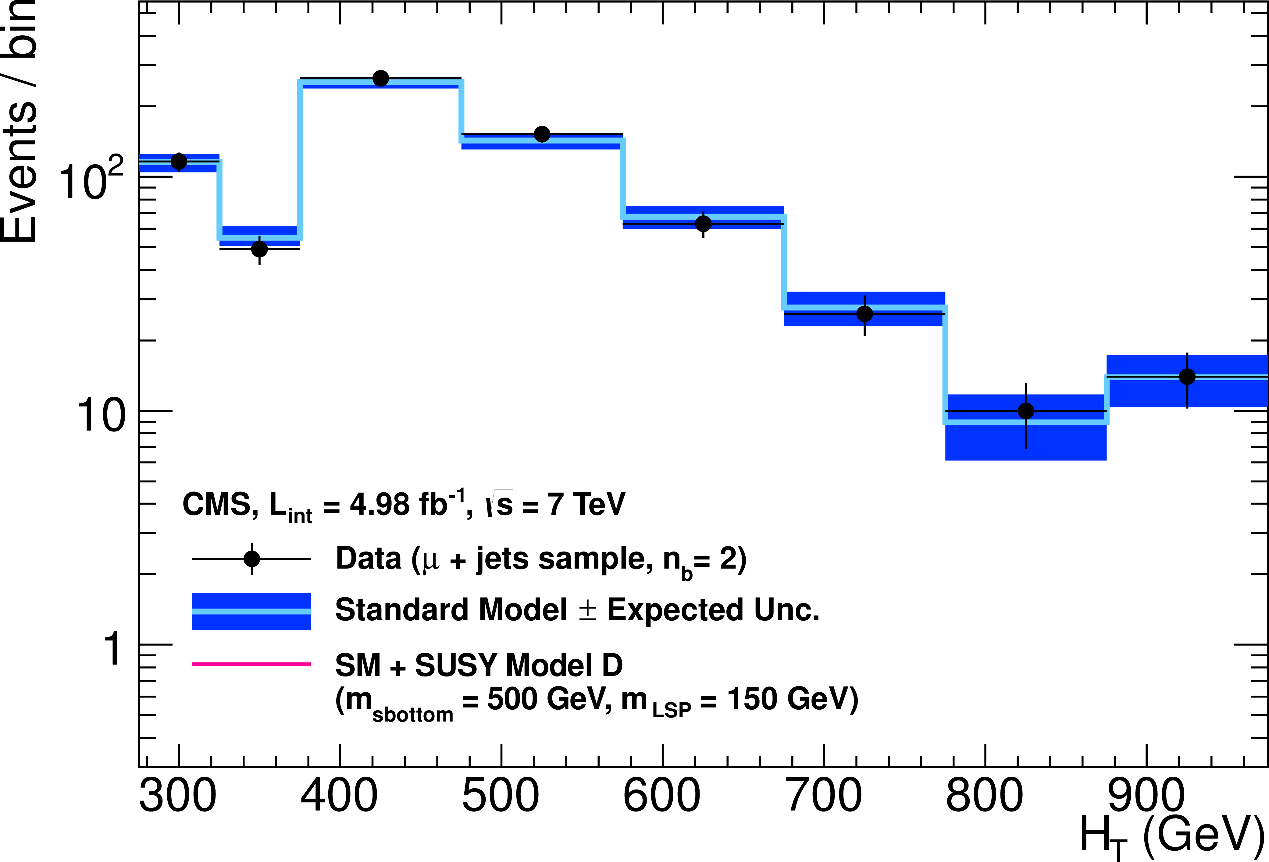
Figure 4-b:
Comparison of the observed yields and SM expectations given by the simultaneous fit in bins of $H_\mathrm {T}$ for the (a) signal region, (b) $ {\mu }$ + jets, (c) $ {\mu \mu } $ + jets, and (d) $ {\gamma } $ + jets samples. Same as Fig. 2, except requiring exactly two reconstructed b-quark jets. The observed event yields in data (black dots) and the expectations and their uncertainties, as determined by the simultaneous fit, for all SM processes (light blue solid line with dark blue bands) are shown. For illustrative purposes only, the signal expectation (magenta solid line) in the signal region for the simplified model $D$ (defined in Section 7.2) with $m_{ \tilde{g} } =$ 500 GeV and $m_\mathrm {LSP} =$ 150 GeV is superimposed on the SM background expectation. |

png pdf |
Figure 4-c:
Comparison of the observed yields and SM expectations given by the simultaneous fit in bins of $H_\mathrm {T}$ for the (a) signal region, (b) $ {\mu }$ + jets, (c) $ {\mu \mu } $ + jets, and (d) $ {\gamma } $ + jets samples. Same as Fig. 2, except requiring exactly two reconstructed b-quark jets. The observed event yields in data (black dots) and the expectations and their uncertainties, as determined by the simultaneous fit, for all SM processes (light blue solid line with dark blue bands) are shown. For illustrative purposes only, the signal expectation (magenta solid line) in the signal region for the simplified model $D$ (defined in Section 7.2) with $m_{ \tilde{g} } =$ 500 GeV and $m_\mathrm {LSP} =$ 150 GeV is superimposed on the SM background expectation. |
png pdf |
Figure 4-d:
Comparison of the observed yields and SM expectations given by the simultaneous fit in bins of $H_\mathrm {T}$ for the (a) signal region, (b) $ {\mu }$ + jets, (c) $ {\mu \mu } $ + jets, and (d) $ {\gamma } $ + jets samples. Same as Fig. 2, except requiring exactly two reconstructed b-quark jets. The observed event yields in data (black dots) and the expectations and their uncertainties, as determined by the simultaneous fit, for all SM processes (light blue solid line with dark blue bands) are shown. For illustrative purposes only, the signal expectation (magenta solid line) in the signal region for the simplified model $D$ (defined in Section 7.2) with $m_{ \tilde{g} } =$ 500 GeV and $m_\mathrm {LSP} =$ 150 GeV is superimposed on the SM background expectation. |

png pdf |
Figure 5-a:
Comparison of the observed yields and SM expectations given by the simultaneous fit in bins of $H_\mathrm {T}$ for the (a) signal region and (b) $ {\mu } $ + jets samples. Same as Fig. 2, except requiring at least three reconstructed b-quark jets. The observed event yields in data (black dots) and the expectations and their uncertainties, as determined by the simultaneous fit, for all SM processes (light blue solid line with dark blue bands) are shown. For illustrative purposes only, the signal expectation (magenta solid line) in the signal region for the simplified model $D$ (defined in Section 7.2) with $m_{ \tilde{g} } =$ 500 GeV and $m_\mathrm {LSP} =$ 150 GeV is superimposed on the SM background expectation. |
png pdf |
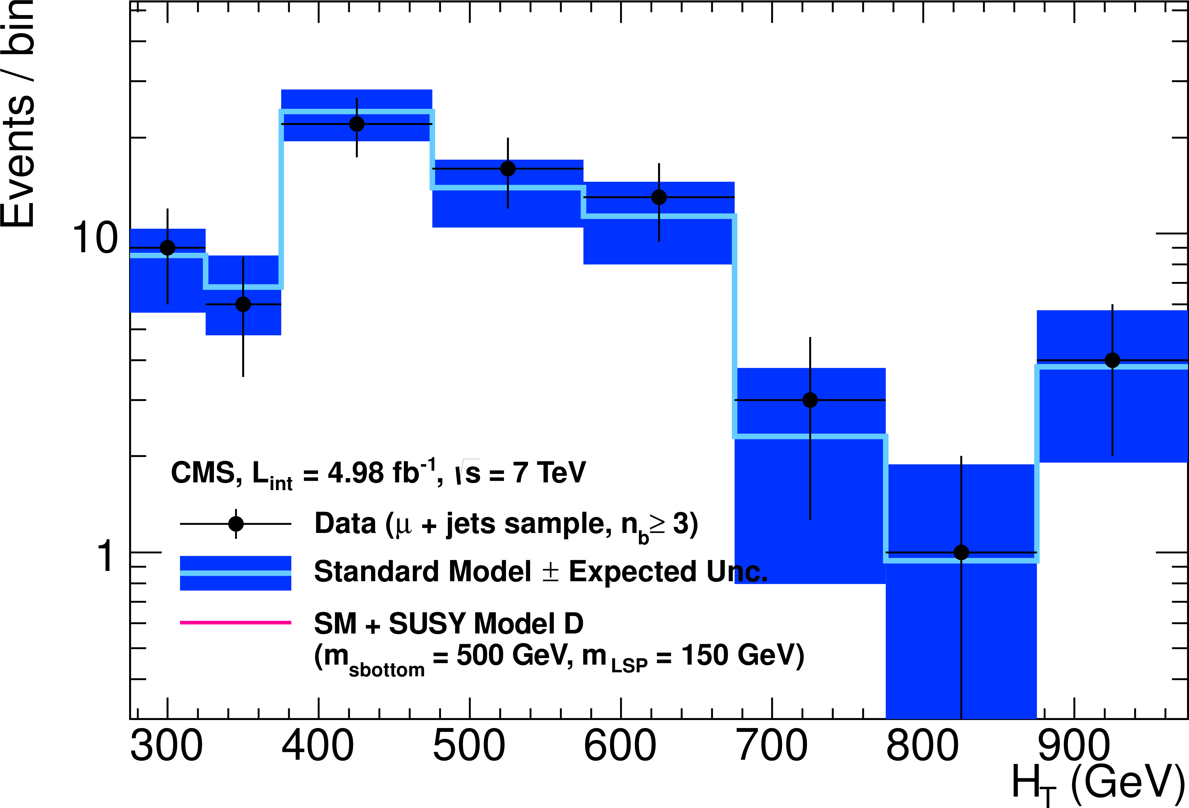
Figure 5-b:
Comparison of the observed yields and SM expectations given by the simultaneous fit in bins of $H_\mathrm {T}$ for the (a) signal region and (b) $ {\mu } $ + jets samples. Same as Fig. 2, except requiring at least three reconstructed b-quark jets. The observed event yields in data (black dots) and the expectations and their uncertainties, as determined by the simultaneous fit, for all SM processes (light blue solid line with dark blue bands) are shown. For illustrative purposes only, the signal expectation (magenta solid line) in the signal region for the simplified model $D$ (defined in Section 7.2) with $m_{ \tilde{g} } =$ 500 GeV and $m_\mathrm {LSP} =$ 150 GeV is superimposed on the SM background expectation. |
png pdf |
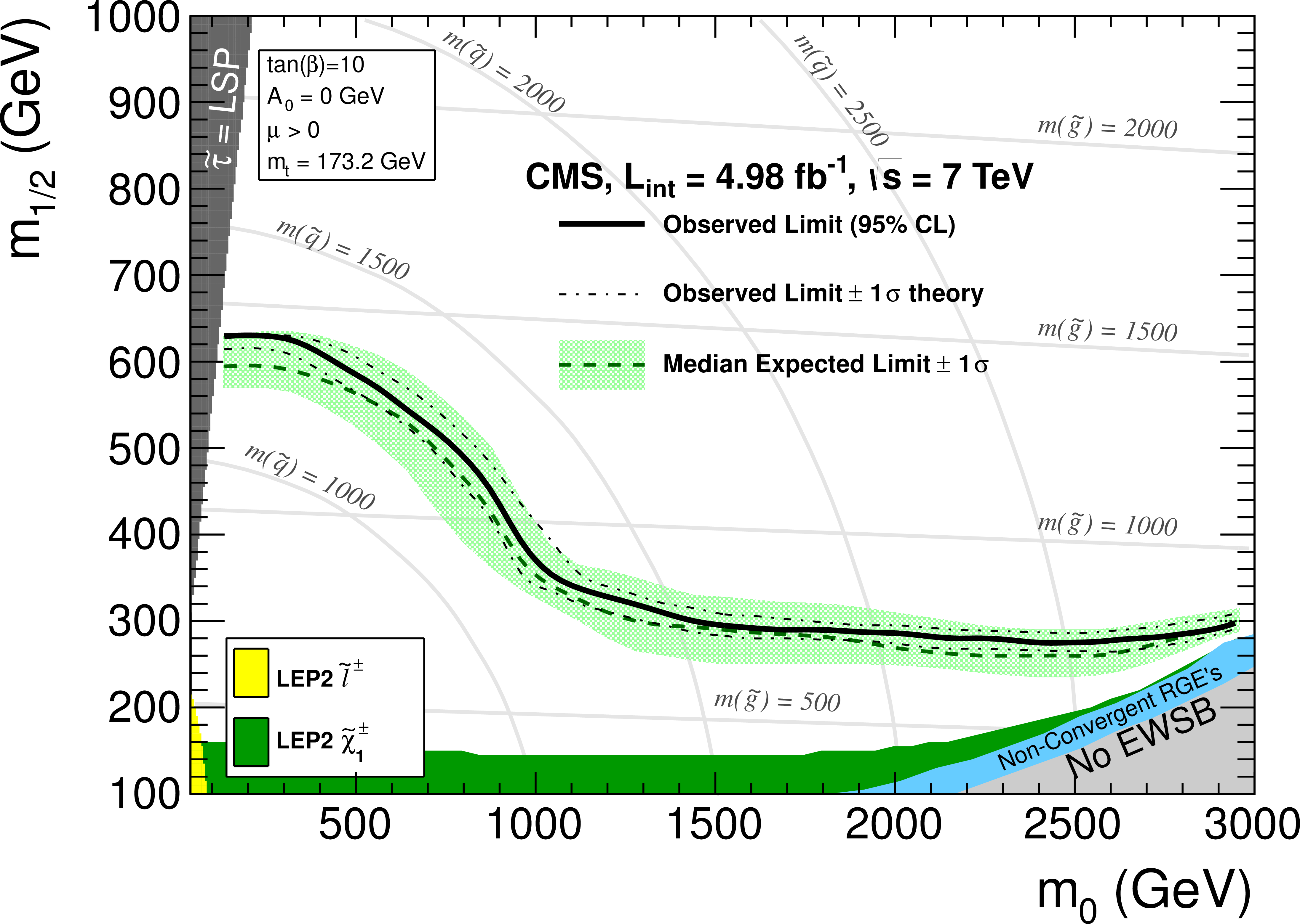
Figure 6:
Exclusion contours at 95% CL in the CMSSM ($m_0, m_{1/2}$) plane ($\tan \beta =$ 10, $A_0 =$ 0, $\mu > $ 0) calculated with NLO+NLL SUSY production cross sections and the CLs method. The solid black line indicates the observed exclusion region. The dotted-dashed black lines represent the observed excluded region when varying the production cross section by its theoretical uncertainty. The expected median exclusion region (green dashed line) $\pm 1 \sigma $ (green band) are also shown. The CMSSM template is taken from Ref.[56]. |

png pdf |
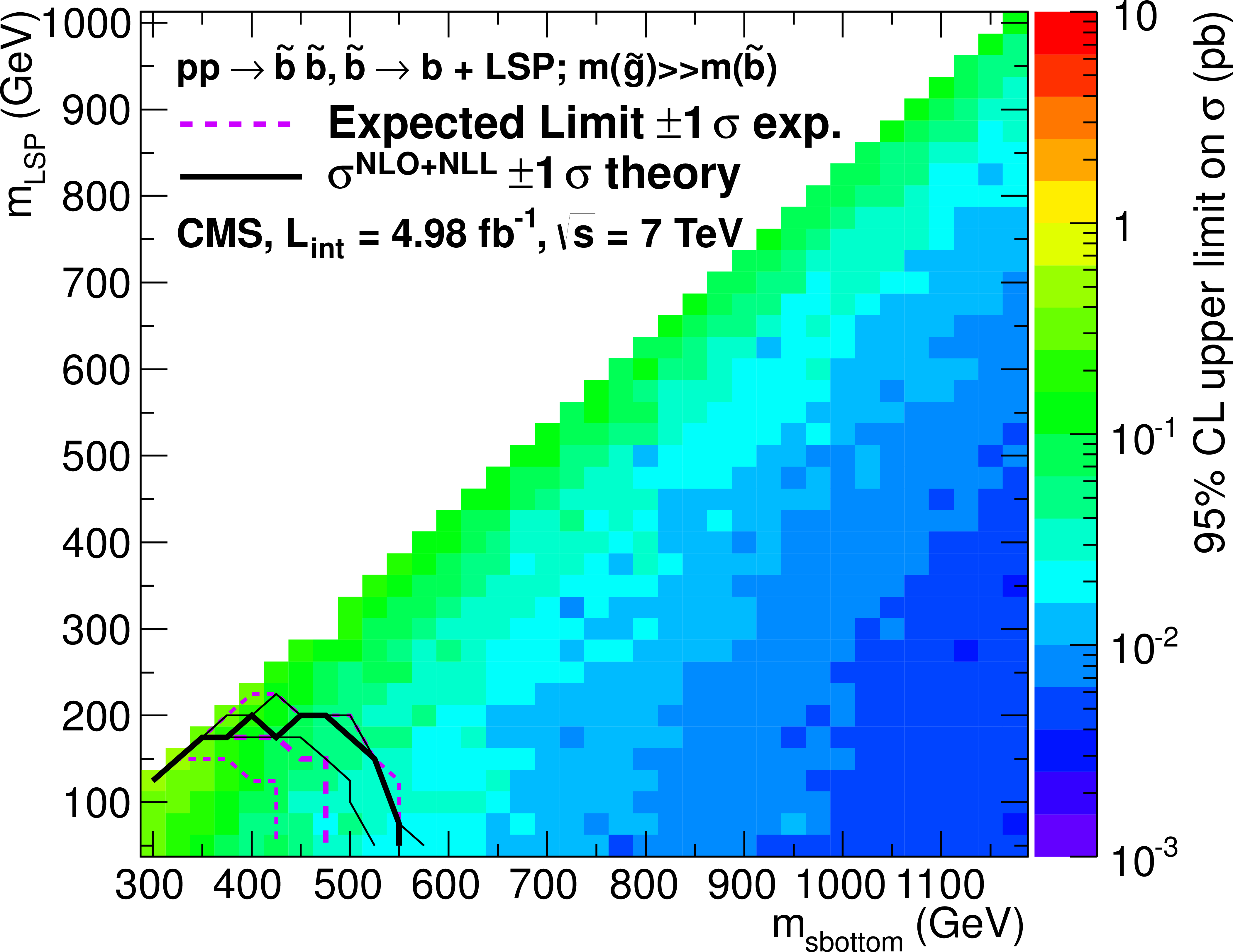
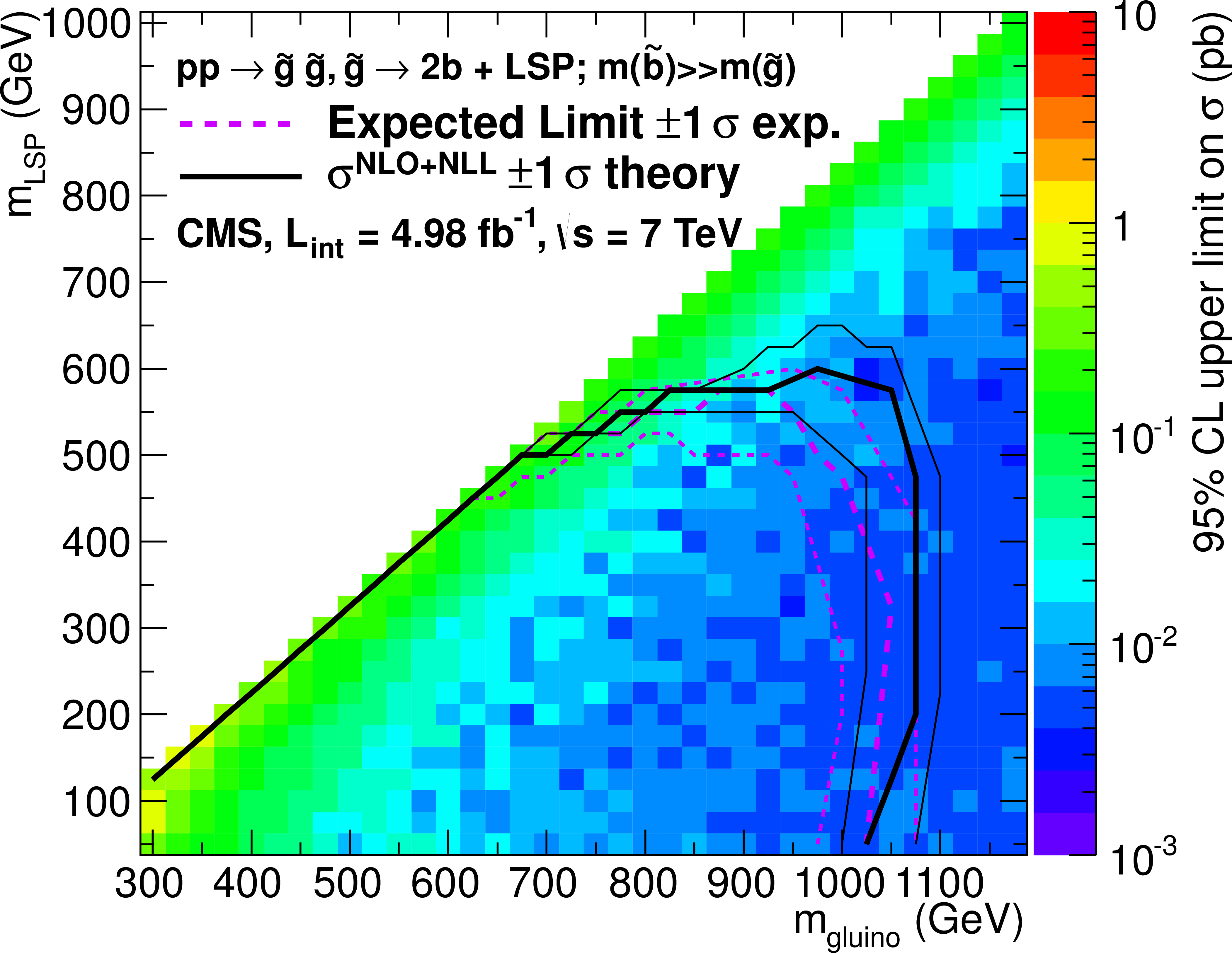
Figure 7-a:
Upper limit on cross section at 95% CL as a function of $m_{ \tilde{q} }$ or $m_{ \tilde{g} } $ and $m_{\rm LSP}$ for various simplified models. The solid thick black line indicates the observed exclusion region assuming NLO+NLL SUSY production cross section. The thin black lines represent the observed excluded region when varying the cross section by its theoretical uncertainty. The dashed purple lines indicate the median (thick line) $\pm 1 \sigma $ (thin lines) expected exclusion regions. The mass ranges considered for models $C$ and $E$ differ from the other models. |

png pdf |
Figure 7-b:
Upper limit on cross section at 95% CL as a function of $m_{ \tilde{q} }$ or $m_{ \tilde{g} } $ and $m_{\rm LSP}$ for various simplified models. The solid thick black line indicates the observed exclusion region assuming NLO+NLL SUSY production cross section. The thin black lines represent the observed excluded region when varying the cross section by its theoretical uncertainty. The dashed purple lines indicate the median (thick line) $\pm 1 \sigma $ (thin lines) expected exclusion regions. The mass ranges considered for models $C$ and $E$ differ from the other models. |
png pdf |
Figure 7-c:
Upper limit on cross section at 95% CL as a function of $m_{ \tilde{q} }$ or $m_{ \tilde{g} } $ and $m_{\rm LSP}$ for various simplified models. The solid thick black line indicates the observed exclusion region assuming NLO+NLL SUSY production cross section. The thin black lines represent the observed excluded region when varying the cross section by its theoretical uncertainty. The dashed purple lines indicate the median (thick line) $\pm 1 \sigma $ (thin lines) expected exclusion regions. The mass ranges considered for models $C$ and $E$ differ from the other models. |
png pdf |
Figure 7-d:
Upper limit on cross section at 95% CL as a function of $m_{ \tilde{q} }$ or $m_{ \tilde{g} } $ and $m_{\rm LSP}$ for various simplified models. The solid thick black line indicates the observed exclusion region assuming NLO+NLL SUSY production cross section. The thin black lines represent the observed excluded region when varying the cross section by its theoretical uncertainty. The dashed purple lines indicate the median (thick line) $\pm 1 \sigma $ (thin lines) expected exclusion regions. The mass ranges considered for models $C$ and $E$ differ from the other models. |

png pdf |
Figure 7-e:
Upper limit on cross section at 95% CL as a function of $m_{ \tilde{q} }$ or $m_{ \tilde{g} } $ and $m_{\rm LSP}$ for various simplified models. The solid thick black line indicates the observed exclusion region assuming NLO+NLL SUSY production cross section. The thin black lines represent the observed excluded region when varying the cross section by its theoretical uncertainty. The dashed purple lines indicate the median (thick line) $\pm 1 \sigma $ (thin lines) expected exclusion regions. The mass ranges considered for models $C$ and $E$ differ from the other models. |
png pdf |
Figure 7-f:
Upper limit on cross section at 95% CL as a function of $m_{ \tilde{q} }$ or $m_{ \tilde{g} } $ and $m_{\rm LSP}$ for various simplified models. The solid thick black line indicates the observed exclusion region assuming NLO+NLL SUSY production cross section. The thin black lines represent the observed excluded region when varying the cross section by its theoretical uncertainty. The dashed purple lines indicate the median (thick line) $\pm 1 \sigma $ (thin lines) expected exclusion regions. The mass ranges considered for models $C$ and $E$ differ from the other models. |

png pdf |
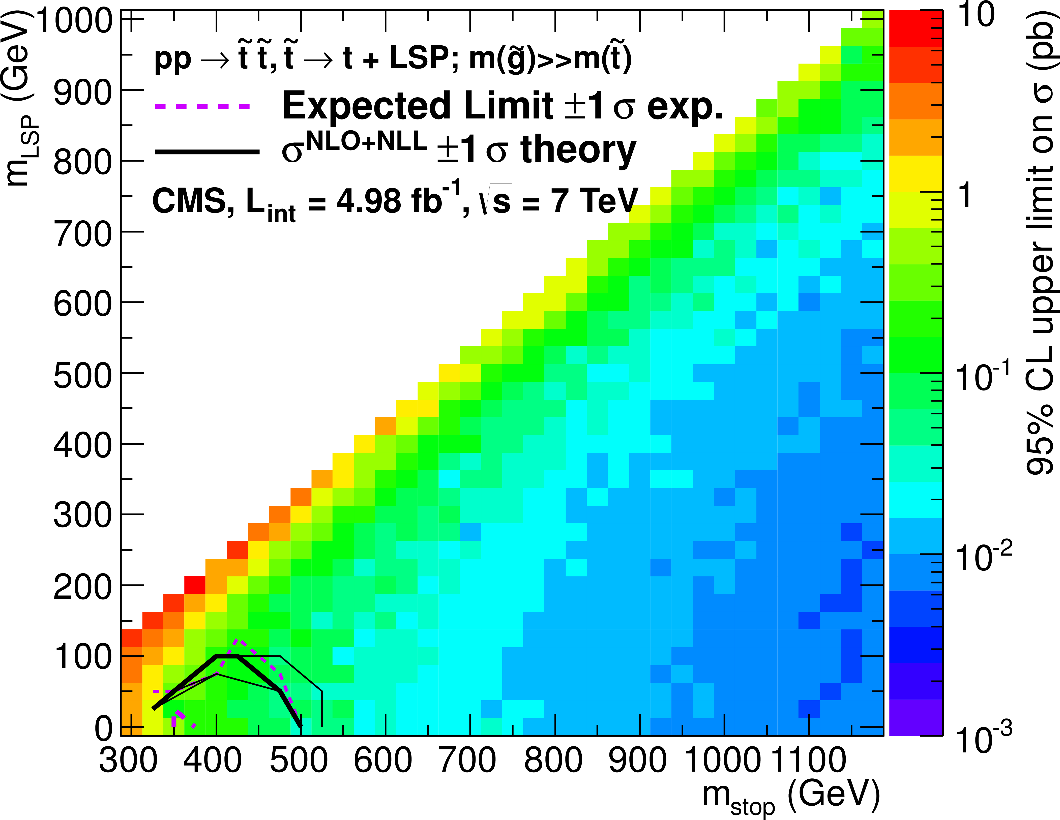
Figure 8:
Excluded cross section versus top squark mass for a model in which pair-produced top squarks decay to two top quarks and two neutralinos of mass $m_{\rm LSP} =$ 50 GeV. The solid blue line indicates the observed cross section upper limit (95% CL) as a function of the top squark mass, $m_{ {\tilde{t}} }$. The dashed orange line and blue band indicate the median expected excluded cross section with experimental uncertainties. The solid black line and grey band indicate the NLO+NLL SUSY top squark pair-production cross section and theoretical uncertainties. |
|
|
Compact Muon Solenoid LHC, CERN |
|

|

|

|

|

|