

Compact Muon Solenoid
LHC, CERN
| CMS-SUS-13-019 ; CERN-PH-EP-2015-017 | ||
| Searches for supersymmetry using the $ M_{\mathrm{T2} } $ variable in hadronic events produced in pp collisions at 8 TeV | ||
| CMS Collaboration | ||
| 15 February 2015 | ||
| J. High Energy Phys. 05 (2015) 078 | ||
| Abstract: Searches for supersymmetry (SUSY) are performed using a sample of hadronic events produced in 8 TeV pp collisions at the CERN LHC. The searches are based on the $M_\mathrm{T2}$ variable, which is a measure of the transverse momentum imbalance in an event. The data were collected with the CMS detector and correspond to an integrated luminosity of 19.5 fb$^{-1}$. Two related searches are performed. The first is an inclusive search based on signal regions defined by the value of the $M_\mathrm{T2}$ variable, the hadronic energy in the event, the jet multiplicity, and the number of jets identified as originating from bottom quarks. The second is a search for a mass peak corresponding to a Higgs boson decaying to a bottom quark-antiquark pair, where the Higgs boson is produced as a decay product of a SUSY particle. For both searches, the principal backgrounds are evaluated with data control samples. No significant excess over the expected number of background events is observed, and exclusion limits on various SUSY models are derived. | ||
| Links: e-print arXiv:1502.04358 [hep-ex] (PDF) ; CDS record ; inSPIRE record ; Public twiki page ; CADI line (restricted) ; | ||
| Figures | |
png pdf |
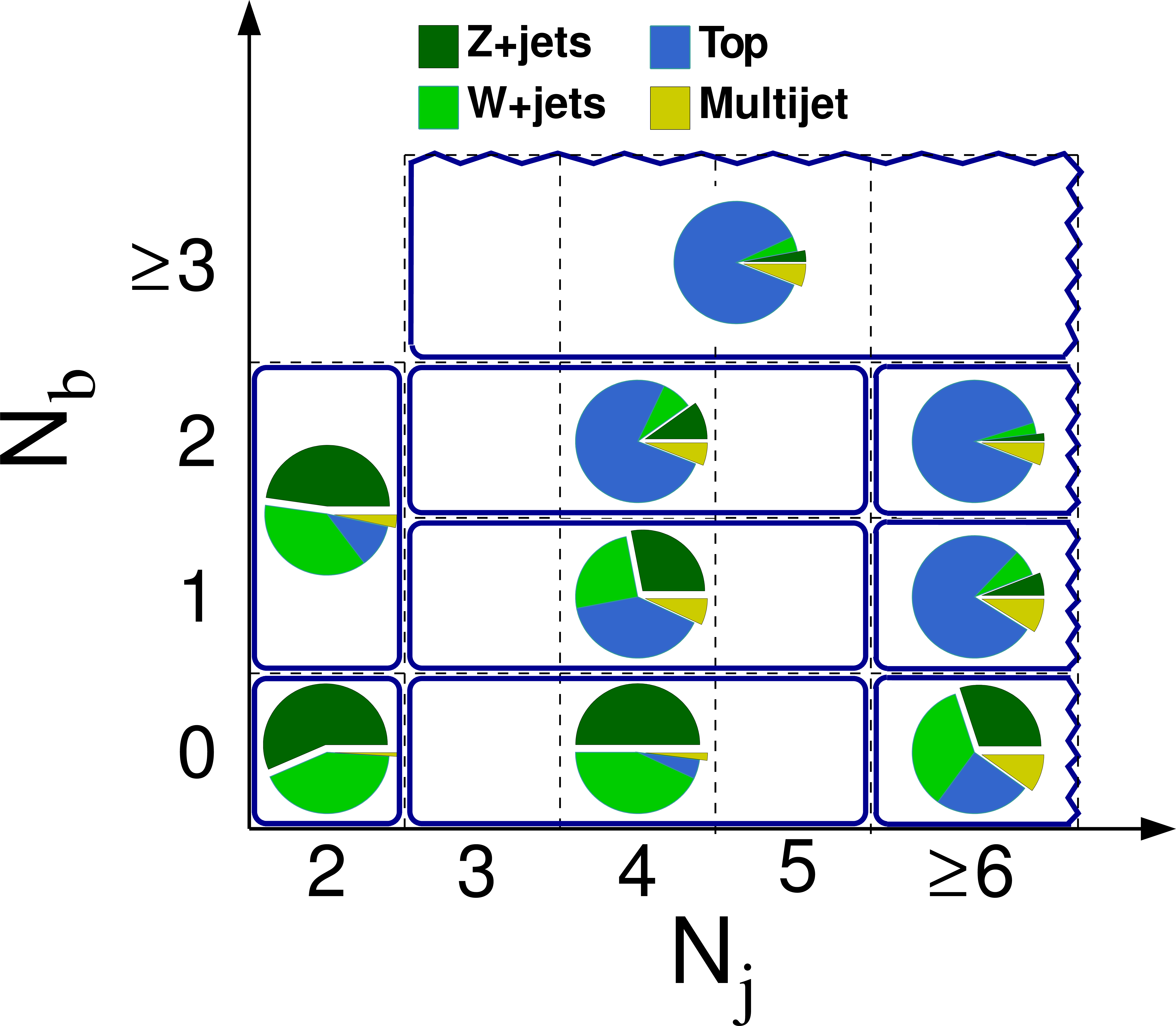
Figure 1-a:
Definition of the topological signal regions in terms of the number of jets $ {N_\mathrm {j}} $ and the number of b-tagged jets $ {N_ {\mathrm {b}} } $ (a), and their subsequent division in terms of $ {H_{\mathrm {T}}} $ and $ {E_{\mathrm {T}}^{\text {miss}}} $ (b). The pie charts illustrate the expected contributions from different SM processes in the different signal regions; they are similar in all three $ {H_{\mathrm {T}}} $ regions. |
png pdf |
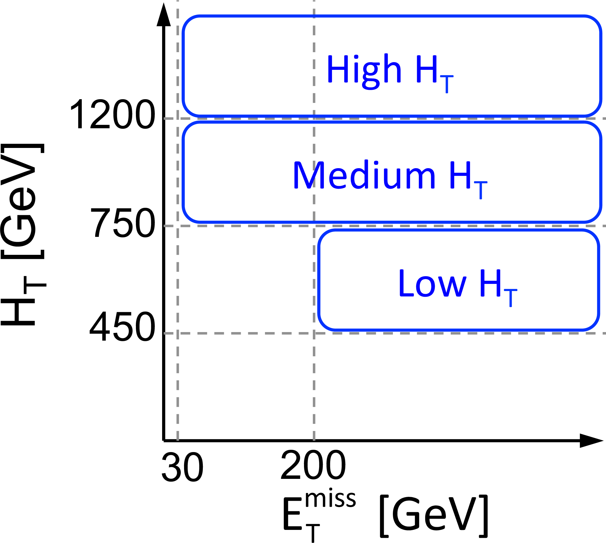
Figure 1-b:
Definition of the topological signal regions in terms of the number of jets $ {N_\mathrm {j}} $ and the number of b-tagged jets $ {N_ {\mathrm {b}} } $ (a), and their subsequent division in terms of $ {H_{\mathrm {T}}} $ and $ {E_{\mathrm {T}}^{\text {miss}}} $ (b). The pie charts illustrate the expected contributions from different SM processes in the different signal regions; they are similar in all three $ {H_{\mathrm {T}}} $ regions. |

png pdf |
Figure 2-a:
Distribution of the $ {M_{\mathrm {T2}}} $ variable after the low-$ {H_{\mathrm {T}}} $ (a), medium-$ {H_{\mathrm {T}}} $ (b), and high-$ {H_{\mathrm {T}}} $ (c) event selections, respectively. The event yields are integrated in the ($ {N_\mathrm {j}} $ , $ {N_ {\mathrm {b}} } $ ) plane over all the topological signal regions, for both simulated and data samples. These plots serve as an illustration of the background composition of the $ {M_{\mathrm {T2}}} $ distributions. |
png pdf |
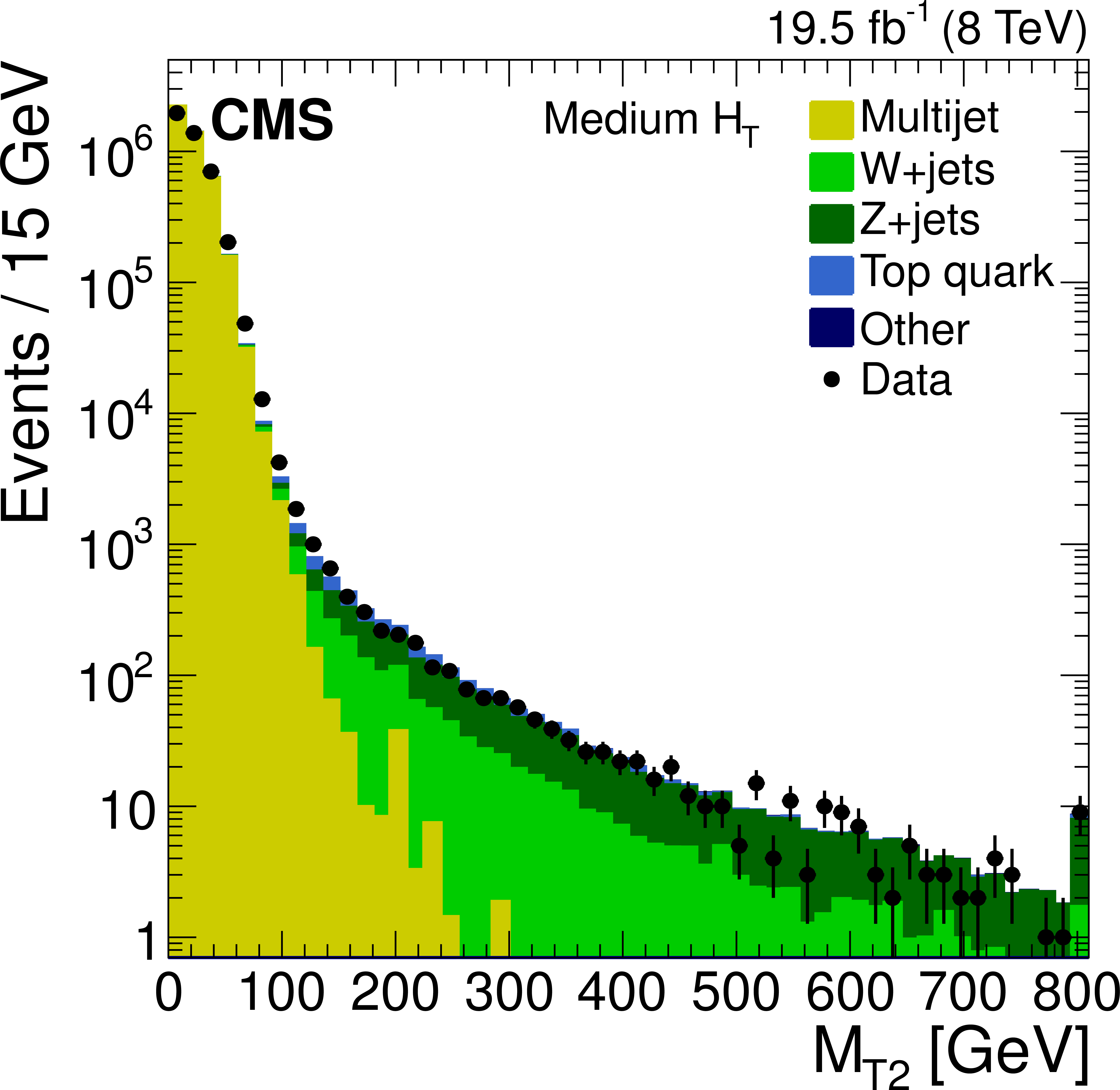
Figure 2-b:
Distribution of the $ {M_{\mathrm {T2}}} $ variable after the low-$ {H_{\mathrm {T}}} $ (a), medium-$ {H_{\mathrm {T}}} $ (b), and high-$ {H_{\mathrm {T}}} $ (c) event selections, respectively. The event yields are integrated in the ($ {N_\mathrm {j}} $ , $ {N_ {\mathrm {b}} } $ ) plane over all the topological signal regions, for both simulated and data samples. These plots serve as an illustration of the background composition of the $ {M_{\mathrm {T2}}} $ distributions. |
png pdf |
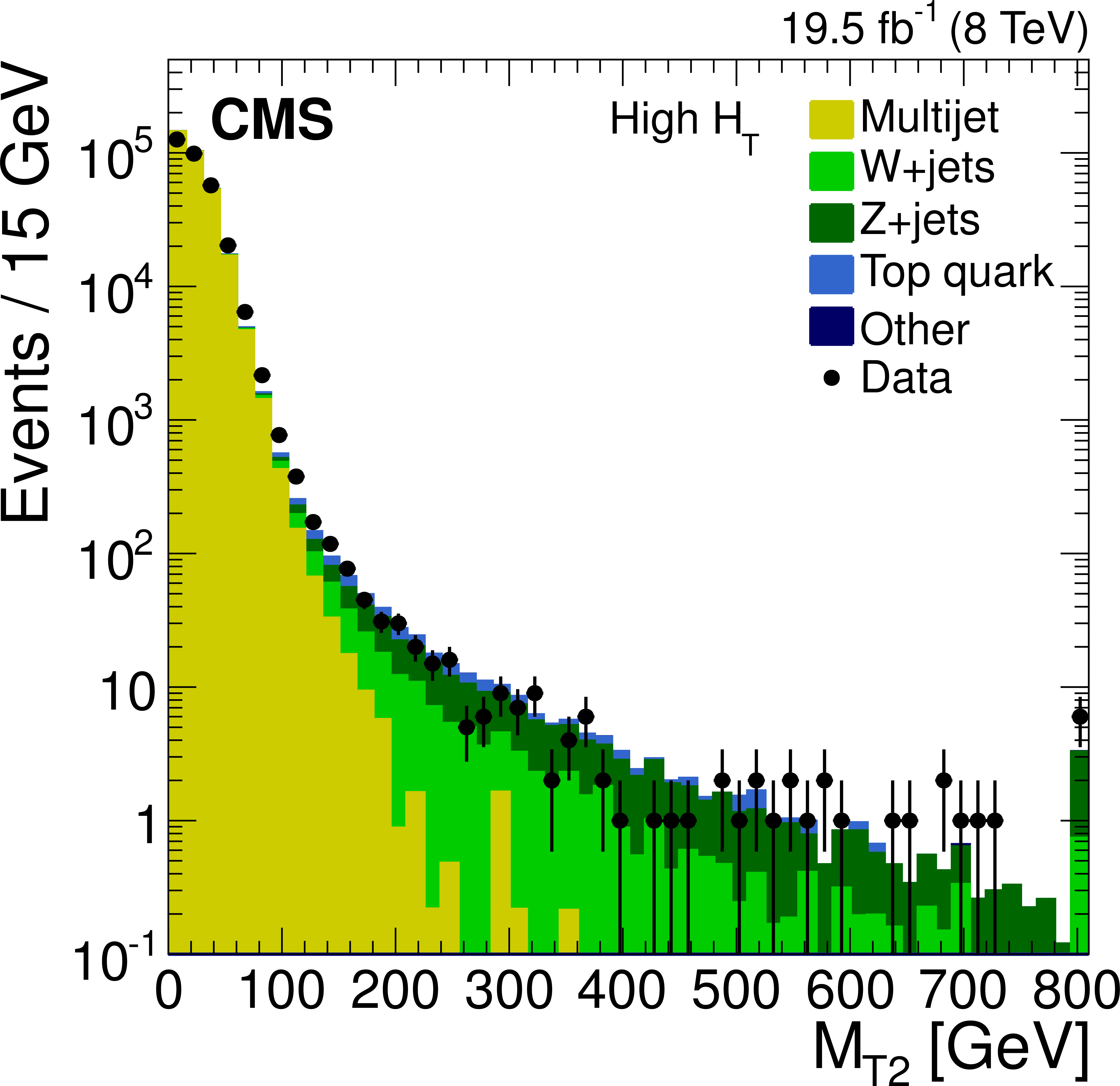
Figure 2-c:
Distribution of the $ {M_{\mathrm {T2}}} $ variable after the low-$ {H_{\mathrm {T}}} $ (a), medium-$ {H_{\mathrm {T}}} $ (b), and high-$ {H_{\mathrm {T}}} $ (c) event selections, respectively. The event yields are integrated in the ($ {N_\mathrm {j}} $ , $ {N_ {\mathrm {b}} } $ ) plane over all the topological signal regions, for both simulated and data samples. These plots serve as an illustration of the background composition of the $ {M_{\mathrm {T2}}} $ distributions. |
png pdf |
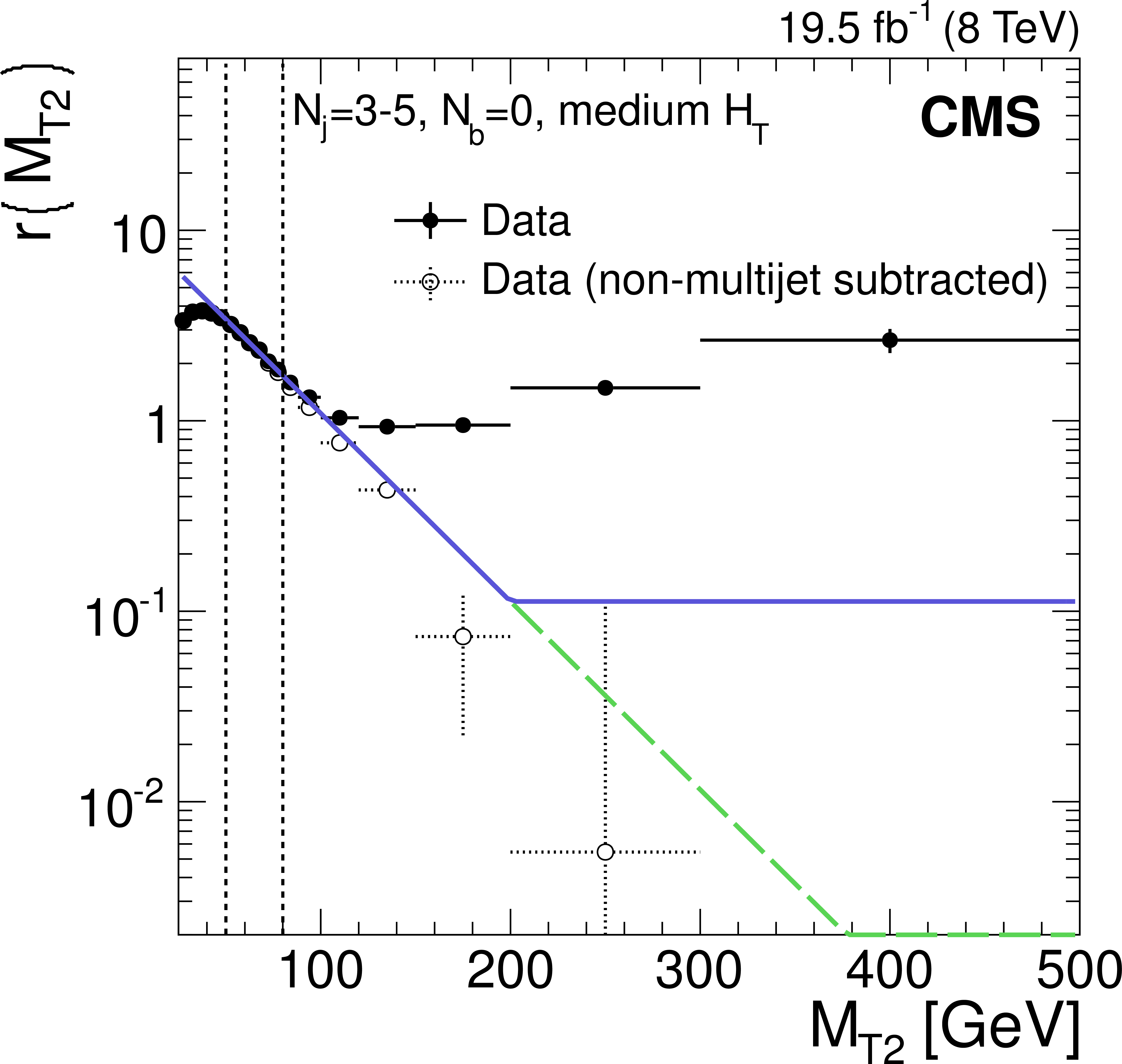
Figure 3:
The ratio $r( {M_{\mathrm {T2}}} )$, described in the text, as a function of $ {M_{\mathrm {T2}}} $ for events satisfying the medium-$ {H_{\mathrm {T}}} $ and the $( {N_\mathrm {j}} =$ 3--5, $ {N_ {\mathrm {b}} } = 0)$ requirements of the inclusive-$ {M_{\mathrm {T2}}} $ search. The solid circle points correspond to simple data yields, while the points with open circles correspond to data after the subtraction of the non-multijet backgrounds, as estimated from simulation. Two different functions, whose exponential components are fitted to the data in the region $50 < {M_{\mathrm {T2}}} < 80 $ GeV, are shown. The green dashed line presents an exponential function, while the blue solid line is the parameterization used in the estimation method. |
png pdf |
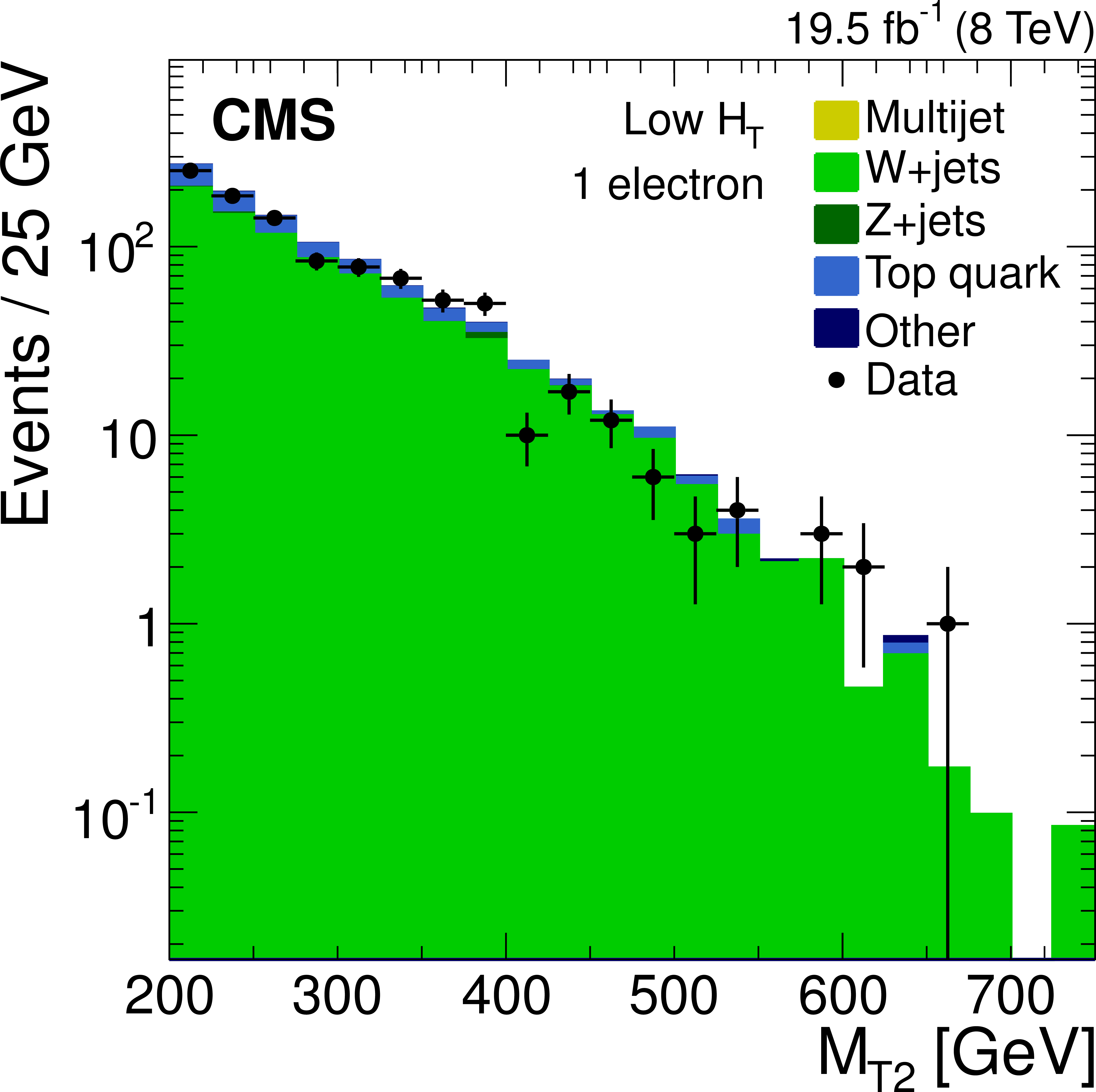
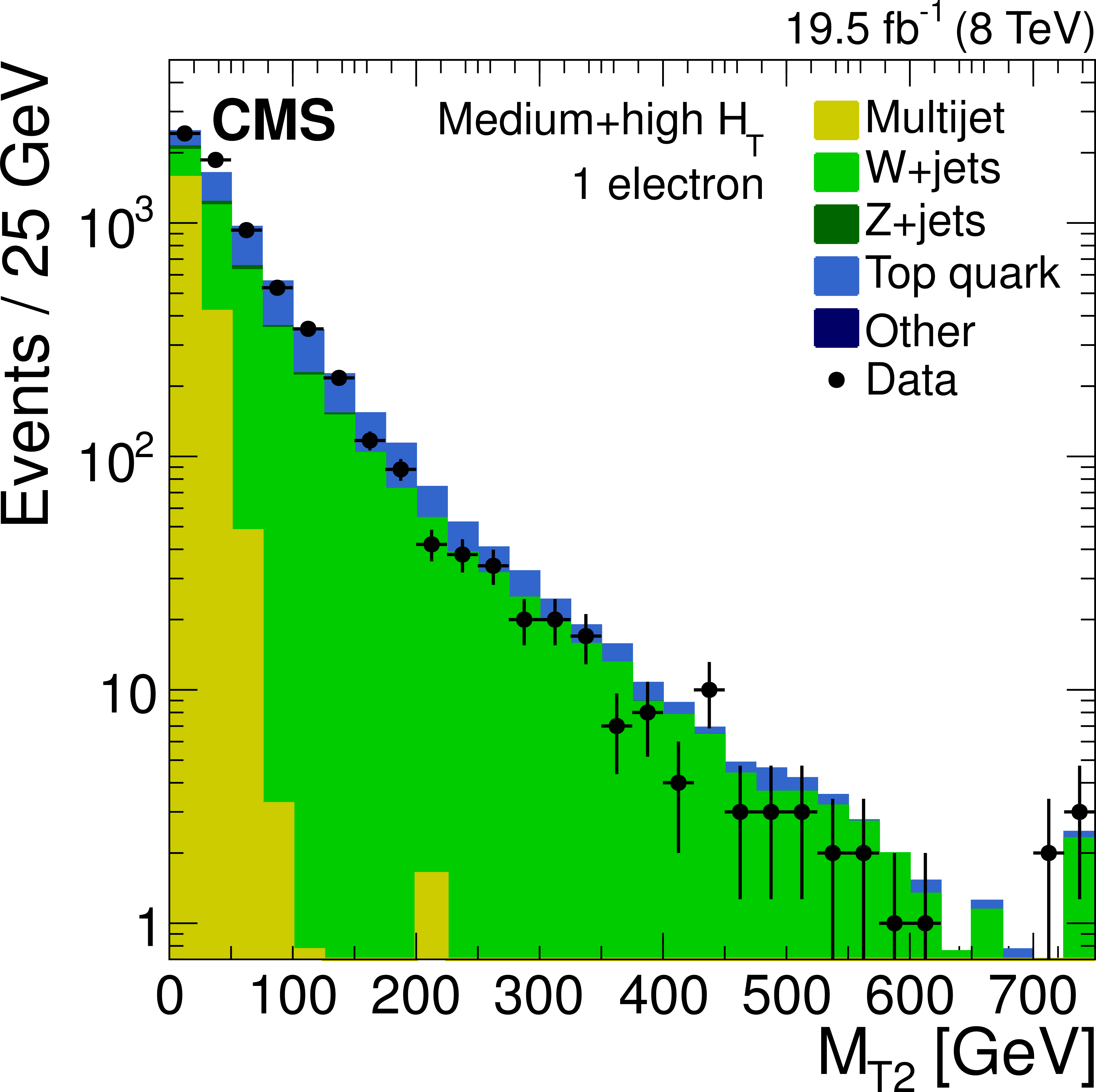
Figure 4-a:
Distribution of the $ {M_{\mathrm {T2}}} $ variable for events with one electron (a,d), one muon (b,e), or one $\tau $ lepton (c,f) in data and simulation. The events satisfy either the low-$ {H_{\mathrm {T}}} $ selection (a,b,c) or either of the medium- and high-$ {H_{\mathrm {T}}} $ selections (d,e,f). They also satisfy the remaining inclusive-$ {M_{\mathrm {T2}}} $ selection requirements, with the exception of the lepton veto. Finally, the condition $ {M_{\mathrm {T}}} < 100 $ GeV is imposed on the charged lepton-$ {E_{\mathrm {T}}^{\text {miss}}} $ system. |
png pdf |
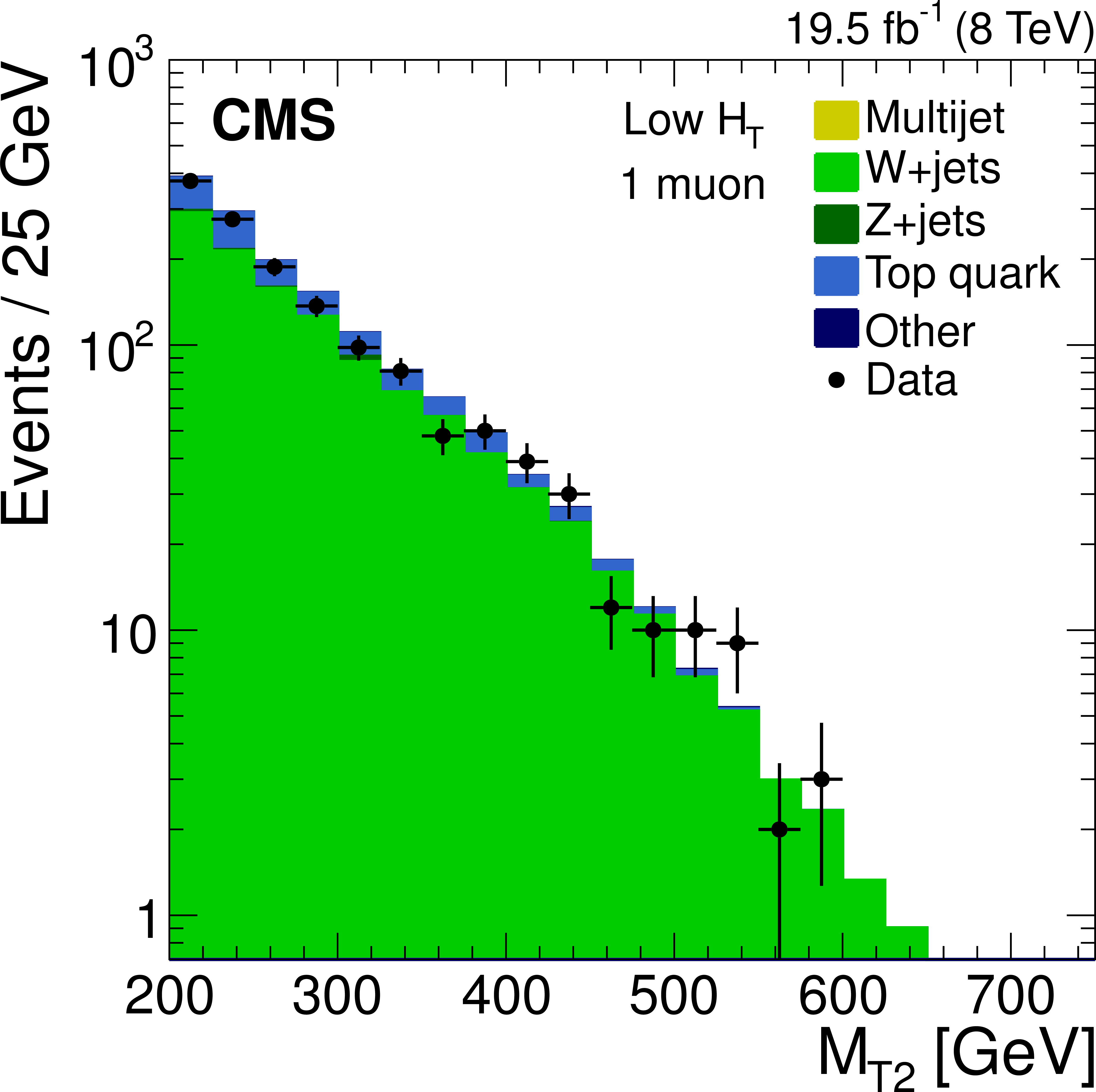
Figure 4-b:
Distribution of the $ {M_{\mathrm {T2}}} $ variable for events with one electron (a,d), one muon (b,e), or one $\tau $ lepton (c,f) in data and simulation. The events satisfy either the low-$ {H_{\mathrm {T}}} $ selection (a,b,c) or either of the medium- and high-$ {H_{\mathrm {T}}} $ selections (d,e,f). They also satisfy the remaining inclusive-$ {M_{\mathrm {T2}}} $ selection requirements, with the exception of the lepton veto. Finally, the condition $ {M_{\mathrm {T}}} < 100 $ GeV is imposed on the charged lepton-$ {E_{\mathrm {T}}^{\text {miss}}} $ system. |
png pdf |
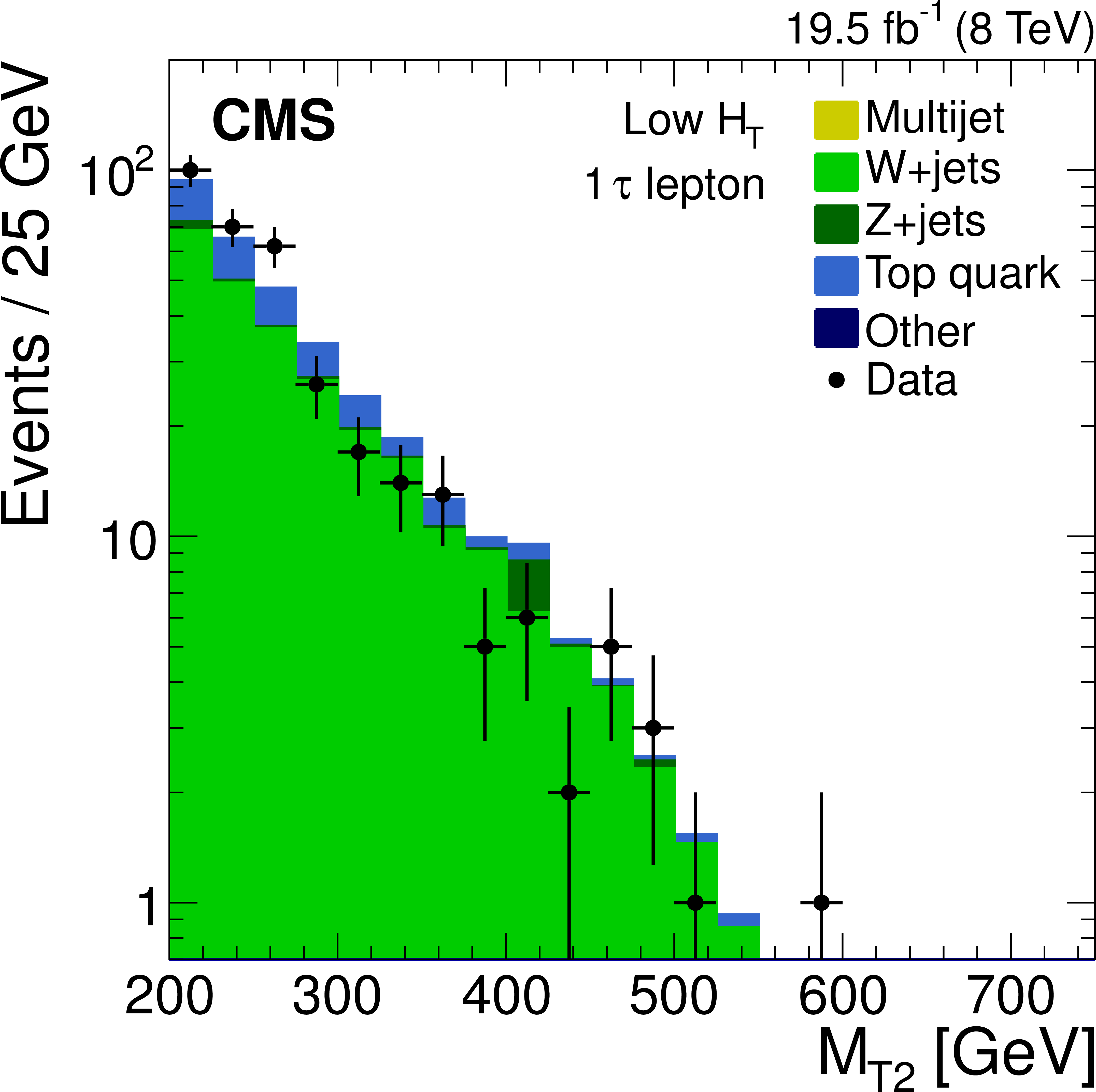
Figure 4-c:
Distribution of the $ {M_{\mathrm {T2}}} $ variable for events with one electron (a,d), one muon (b,e), or one $\tau $ lepton (c,f) in data and simulation. The events satisfy either the low-$ {H_{\mathrm {T}}} $ selection (a,b,c) or either of the medium- and high-$ {H_{\mathrm {T}}} $ selections (d,e,f). They also satisfy the remaining inclusive-$ {M_{\mathrm {T2}}} $ selection requirements, with the exception of the lepton veto. Finally, the condition $ {M_{\mathrm {T}}} < 100 $ GeV is imposed on the charged lepton-$ {E_{\mathrm {T}}^{\text {miss}}} $ system. |
png pdf |
Figure 4-d:
Distribution of the $ {M_{\mathrm {T2}}} $ variable for events with one electron (a,d), one muon (b,e), or one $\tau $ lepton (c,f) in data and simulation. The events satisfy either the low-$ {H_{\mathrm {T}}} $ selection (a,b,c) or either of the medium- and high-$ {H_{\mathrm {T}}} $ selections (d,e,f). They also satisfy the remaining inclusive-$ {M_{\mathrm {T2}}} $ selection requirements, with the exception of the lepton veto. Finally, the condition $ {M_{\mathrm {T}}} < 100 $ GeV is imposed on the charged lepton-$ {E_{\mathrm {T}}^{\text {miss}}} $ system. |
png pdf |
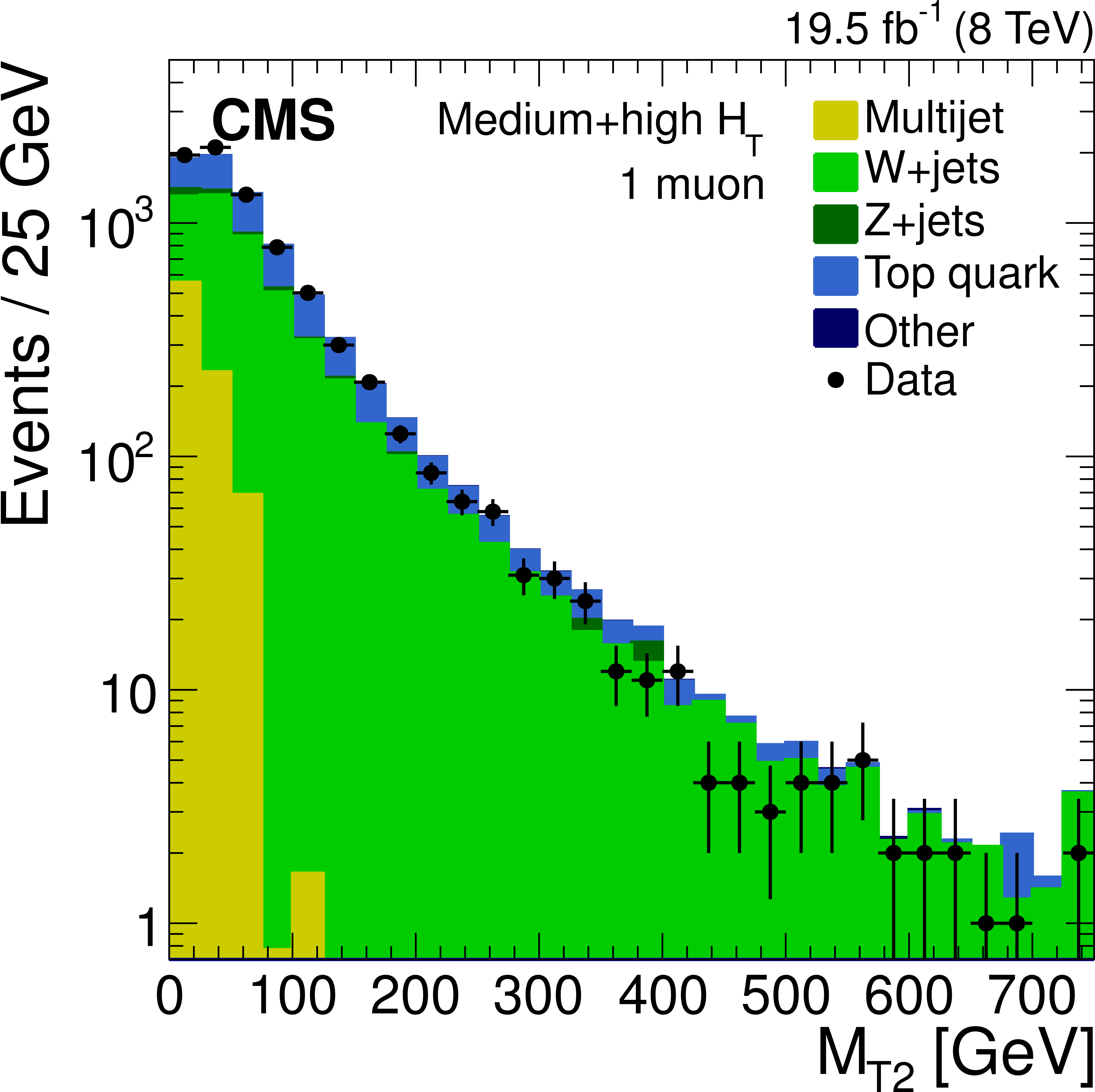
Figure 4-e:
Distribution of the $ {M_{\mathrm {T2}}} $ variable for events with one electron (a,d), one muon (b,e), or one $\tau $ lepton (c,f) in data and simulation. The events satisfy either the low-$ {H_{\mathrm {T}}} $ selection (a,b,c) or either of the medium- and high-$ {H_{\mathrm {T}}} $ selections (d,e,f). They also satisfy the remaining inclusive-$ {M_{\mathrm {T2}}} $ selection requirements, with the exception of the lepton veto. Finally, the condition $ {M_{\mathrm {T}}} < 100 $ GeV is imposed on the charged lepton-$ {E_{\mathrm {T}}^{\text {miss}}} $ system. |
png pdf |
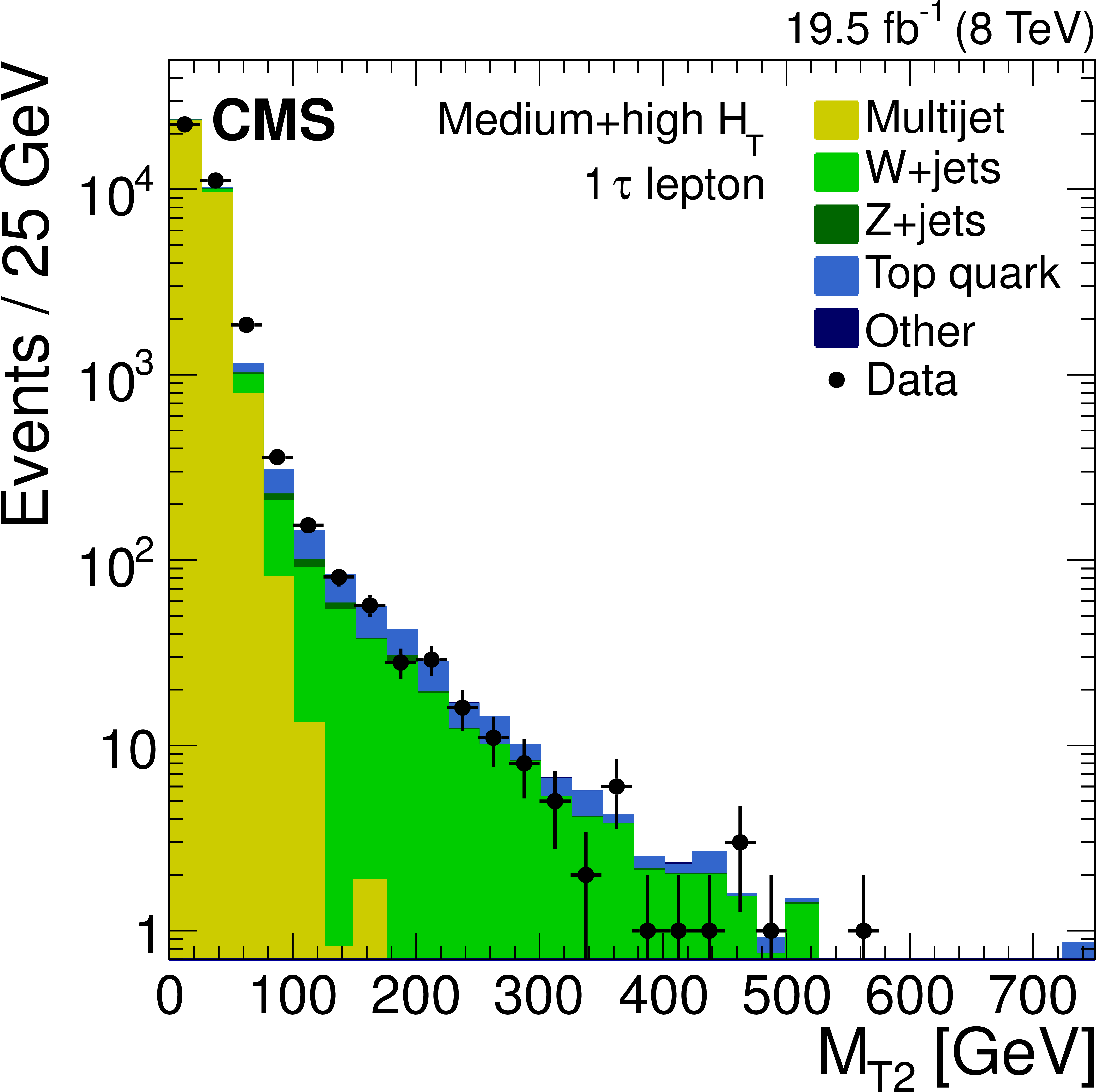
Figure 4-f:
Distribution of the $ {M_{\mathrm {T2}}} $ variable for events with one electron (a,d), one muon (b,e), or one $\tau $ lepton (c,f) in data and simulation. The events satisfy either the low-$ {H_{\mathrm {T}}} $ selection (a,b,c) or either of the medium- and high-$ {H_{\mathrm {T}}} $ selections (d,e,f). They also satisfy the remaining inclusive-$ {M_{\mathrm {T2}}} $ selection requirements, with the exception of the lepton veto. Finally, the condition $ {M_{\mathrm {T}}} < 100 $ GeV is imposed on the charged lepton-$ {E_{\mathrm {T}}^{\text {miss}}} $ system. |
png pdf |
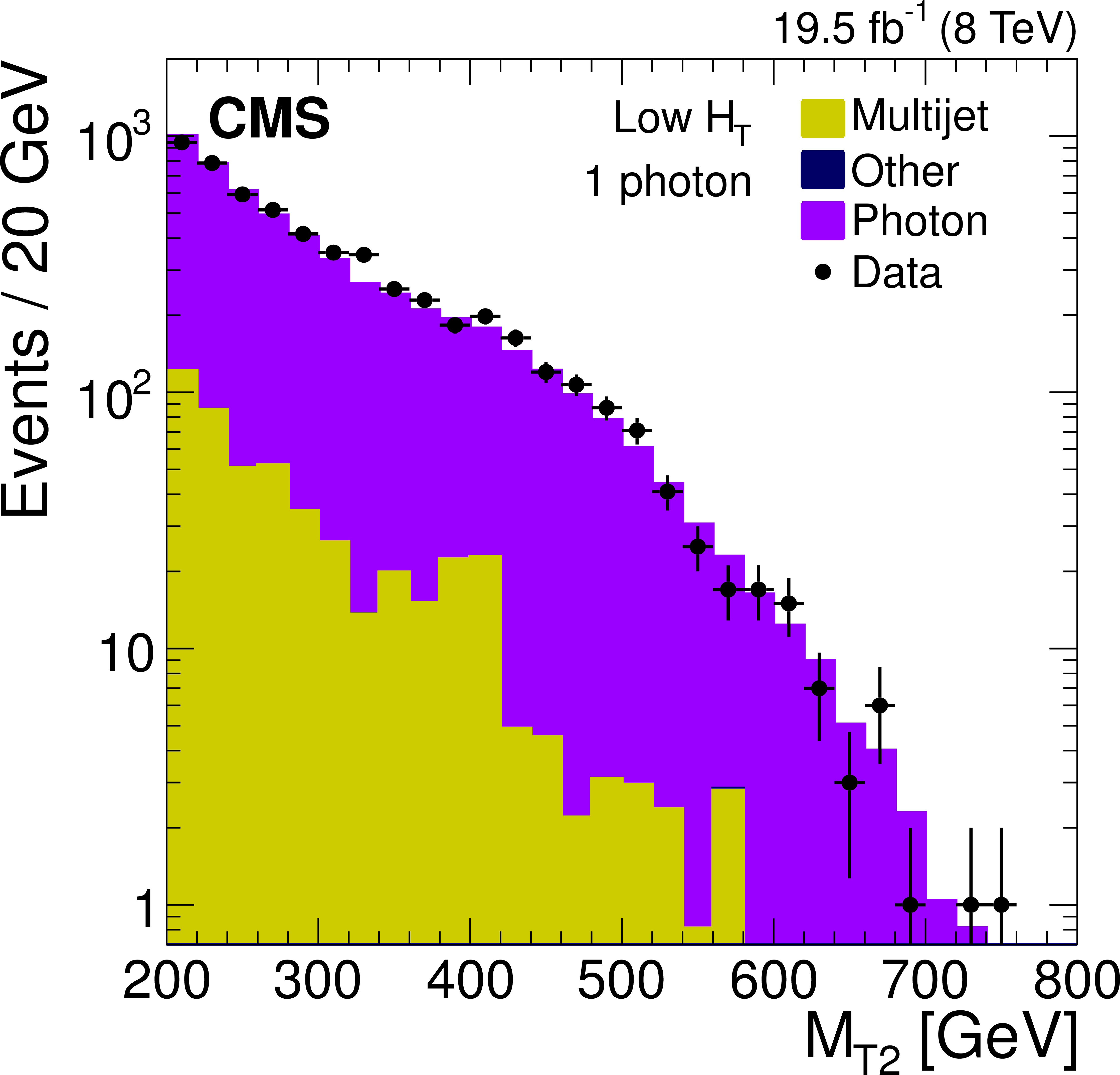
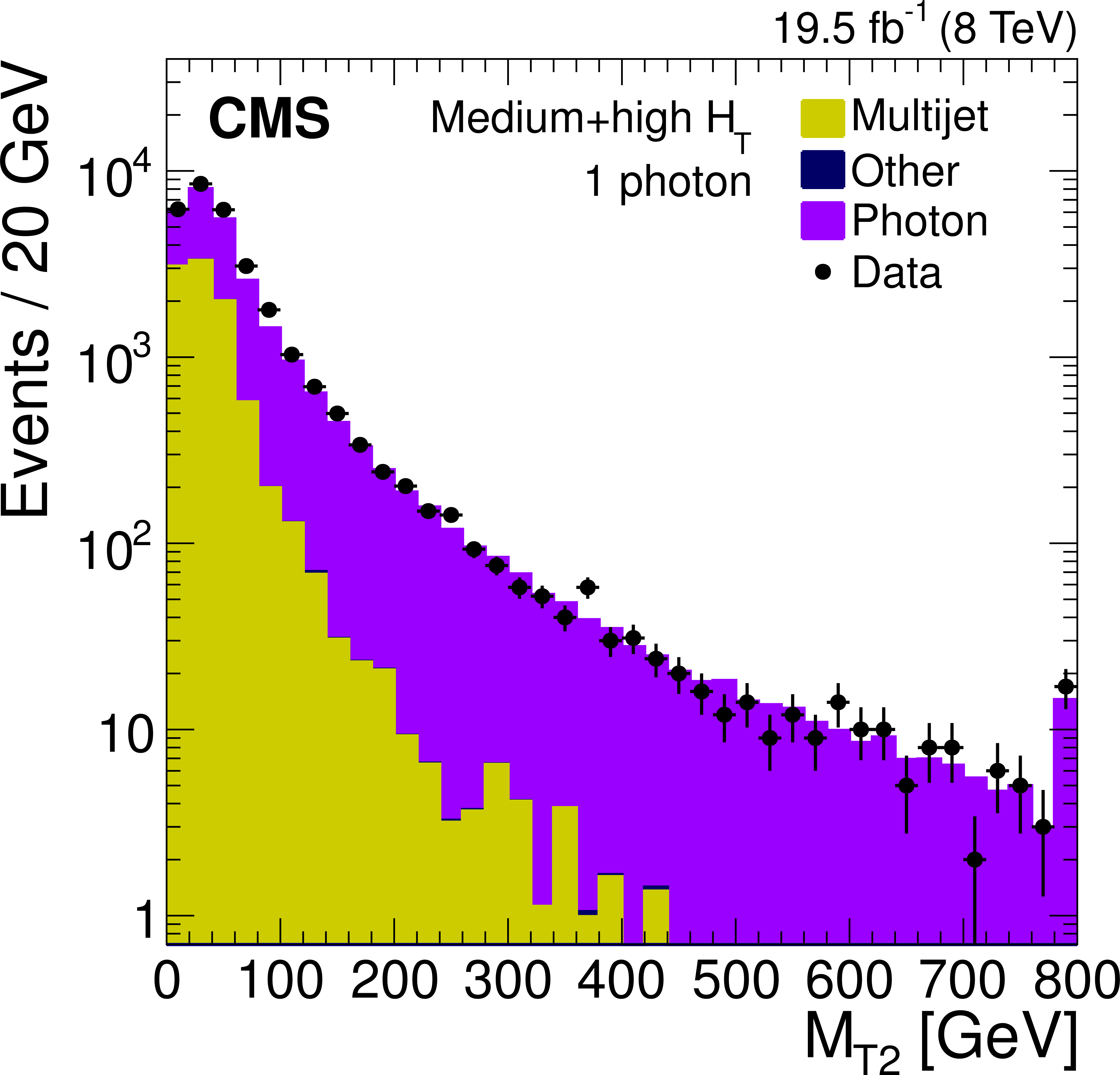
Figure 5-a:
Distribution of the $ {M_{\mathrm {T2}}} $ variable for data and simulation after requiring the presence of one photon, $ {N_ {\mathrm {b}} } =0$, and the remainder of the inclusive-$ {M_{\mathrm {T2}}} $ selection criteria. Events satisfying the low-$ {H_{\mathrm {T}}} $ selection (a), and the medium- and high-$ {H_{\mathrm {T}}} $ selections (b) are shown. For these results, $ {M_{\mathrm {T2}}} $ is calculated after adding the photon $ {p_{\mathrm {T}}} $ to the $ {E_{\mathrm {T}}^{\text {miss}}} $ vector. |
png pdf |
Figure 5-b:
Distribution of the $ {M_{\mathrm {T2}}} $ variable for data and simulation after requiring the presence of one photon, $ {N_ {\mathrm {b}} } =0$, and the remainder of the inclusive-$ {M_{\mathrm {T2}}} $ selection criteria. Events satisfying the low-$ {H_{\mathrm {T}}} $ selection (a), and the medium- and high-$ {H_{\mathrm {T}}} $ selections (b) are shown. For these results, $ {M_{\mathrm {T2}}} $ is calculated after adding the photon $ {p_{\mathrm {T}}} $ to the $ {E_{\mathrm {T}}^{\text {miss}}} $ vector. |
png pdf |
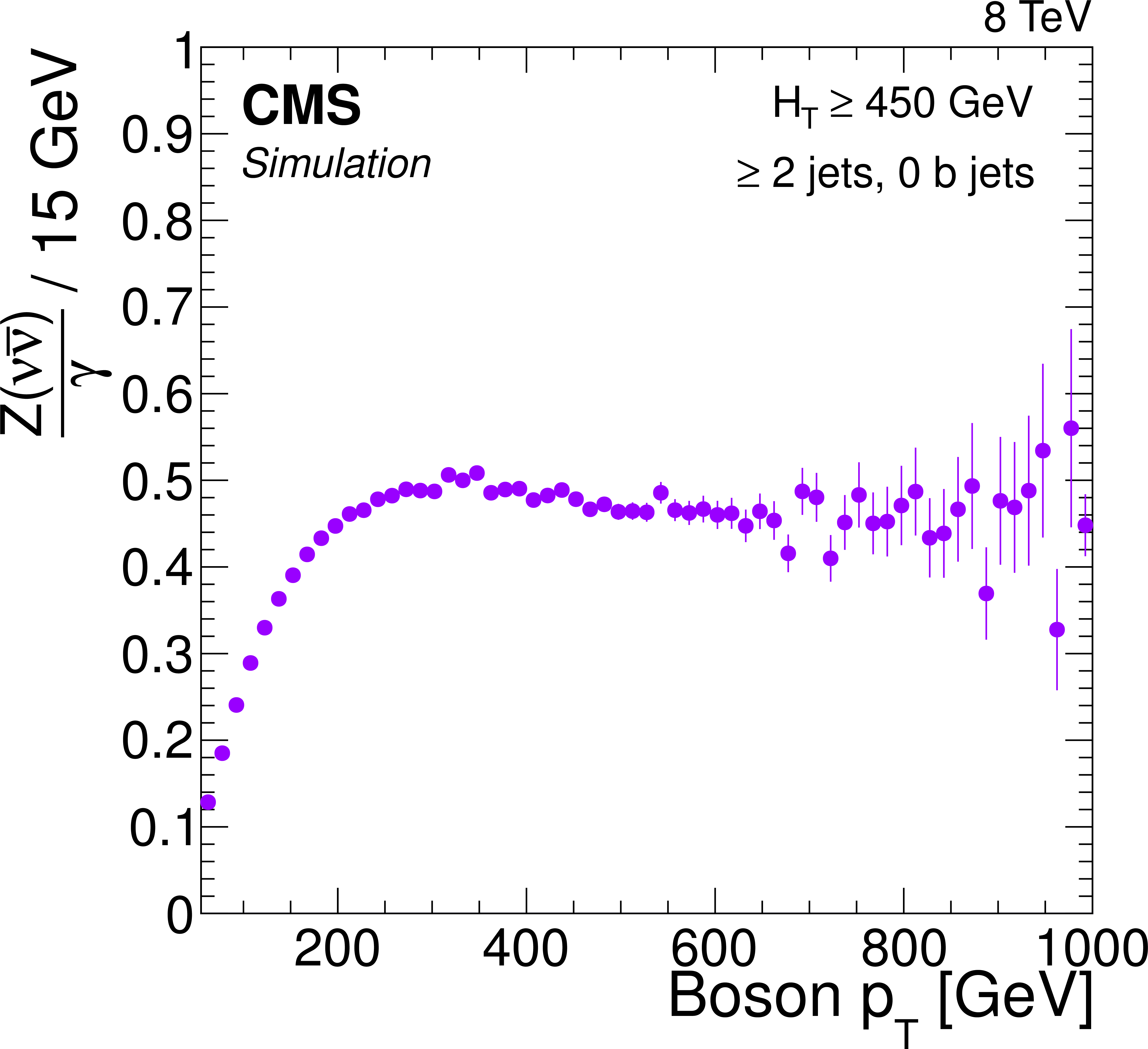
Figure 6:
Ratio $ { {\mathrm {Z}} (\nu {\overline {\nu }} )/\gamma } $ of events satisfying the event selection of the ($ {N_\mathrm {j}} \ge 2$, $ {N_ {\mathrm {b}} } =0$) signal region as a function of the boson $ {p_{\mathrm {T}}} $. The events are summed inclusively in all $ {H_{\mathrm {T}}} $ sub-regions with $ {H_{\mathrm {T}}} \ge 450 $ GeV. The ratio is obtained in simulated events after the photon momentum is included in the $ {E_{\mathrm {T}}^{\text {miss}}} $ calculation. |
png pdf |
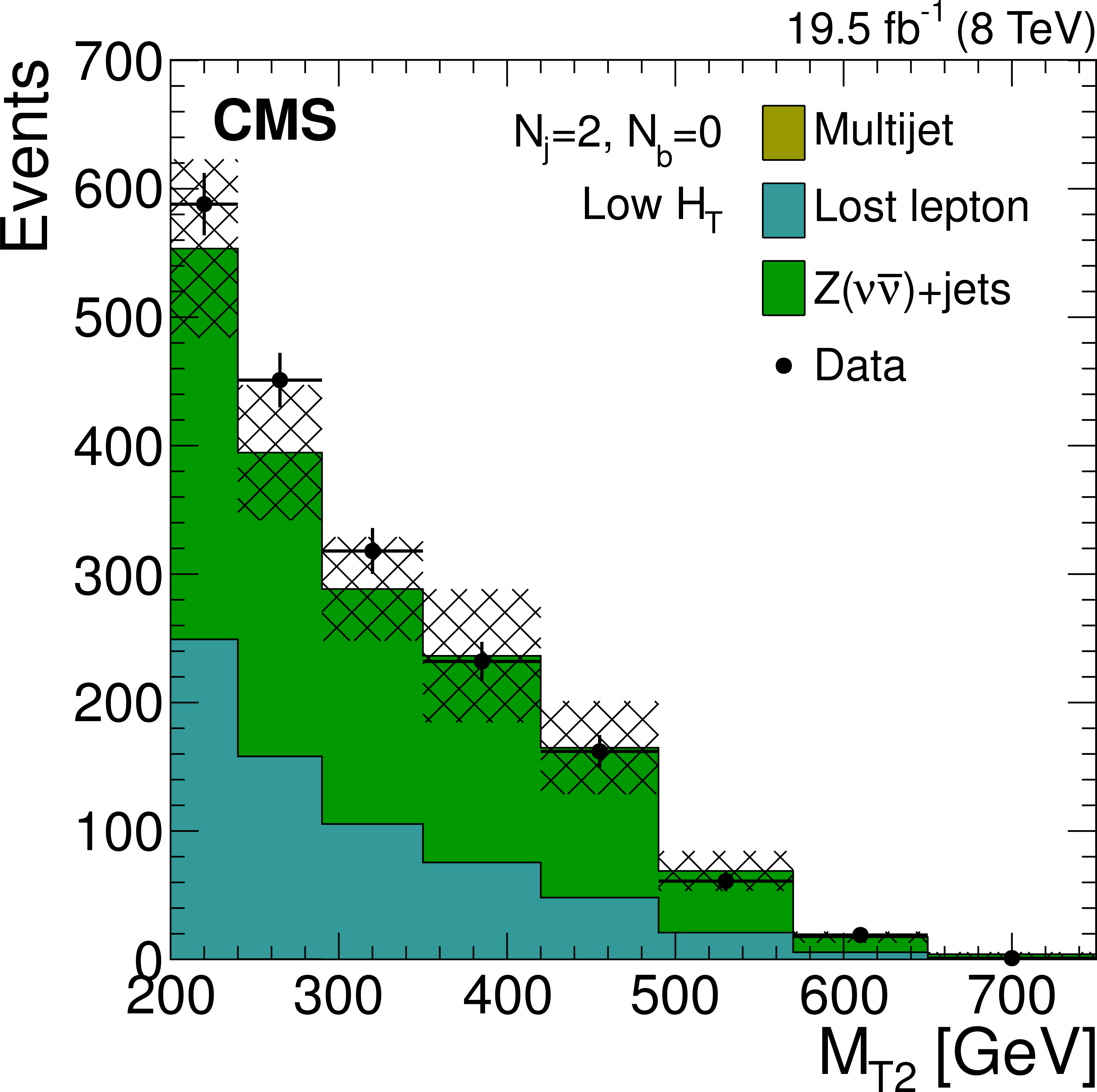
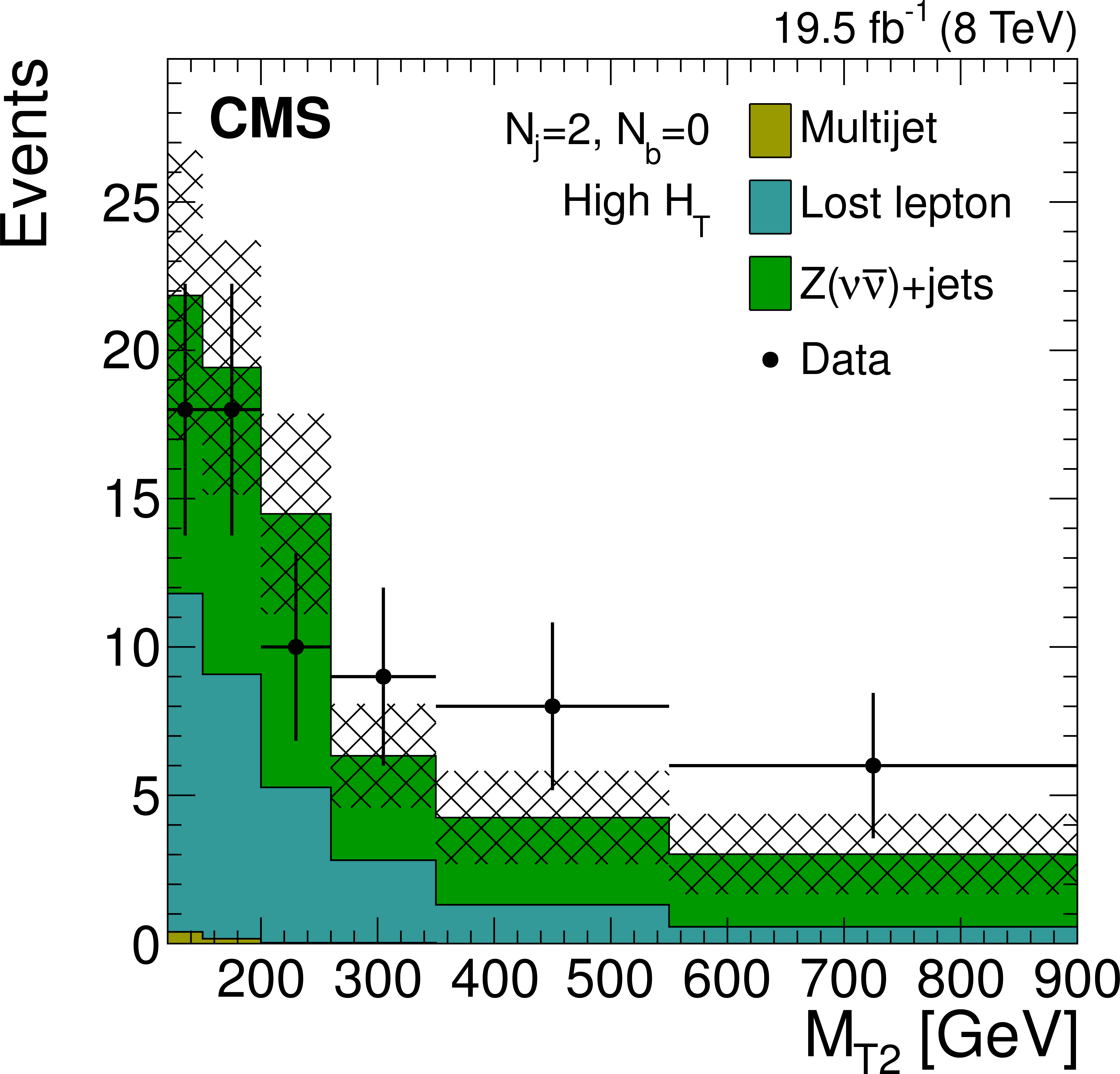
Figure 7-a:
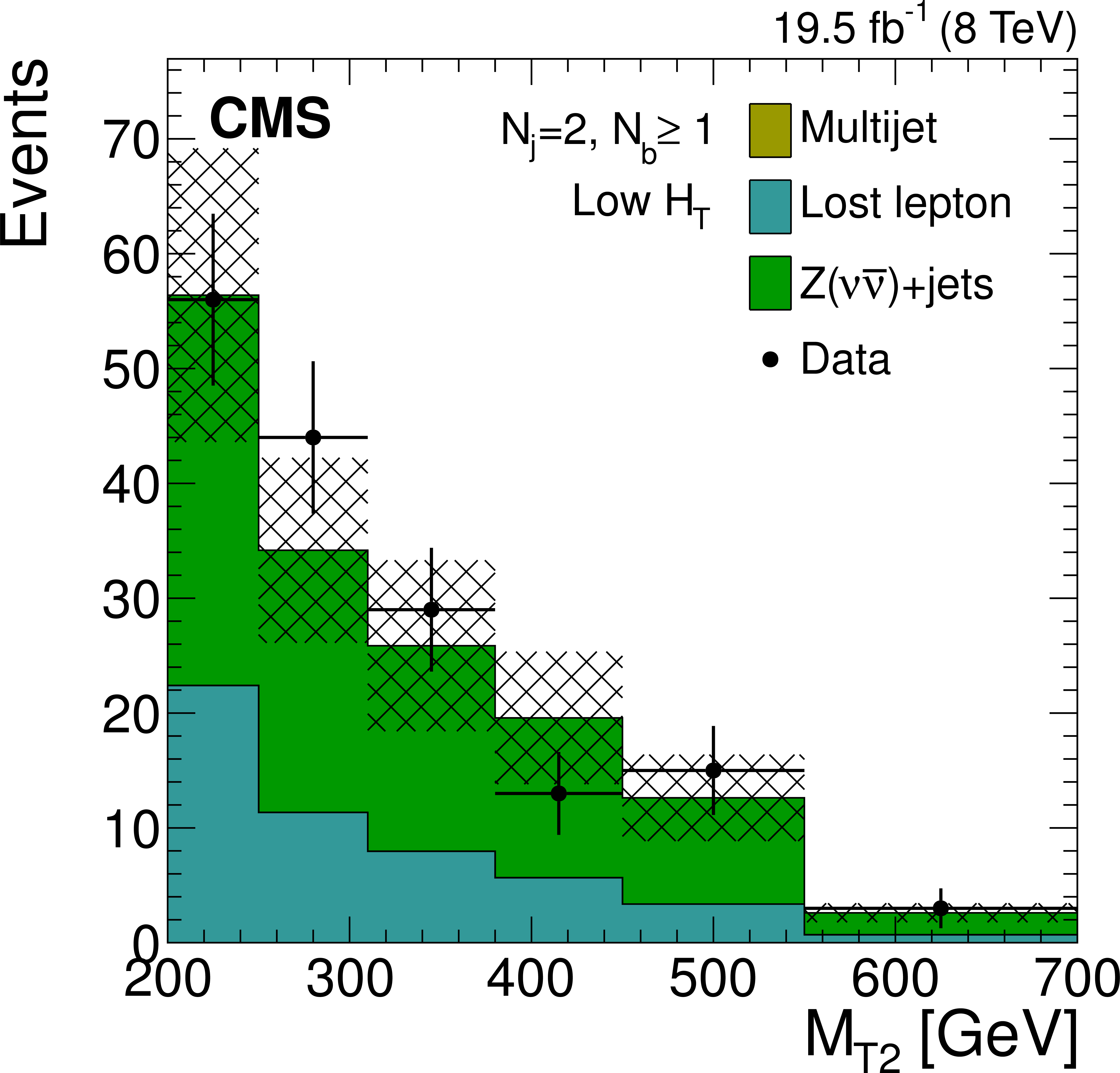
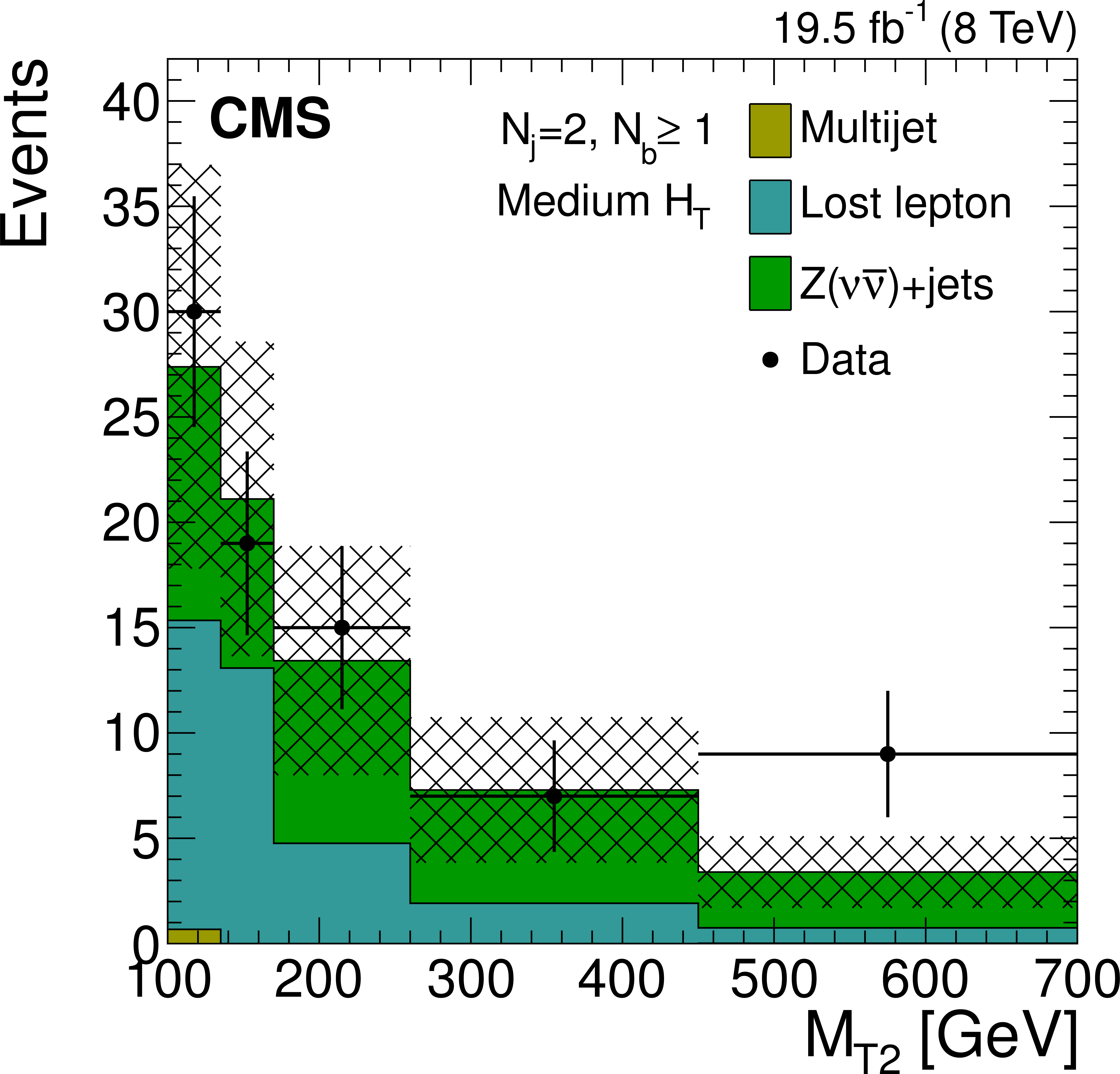
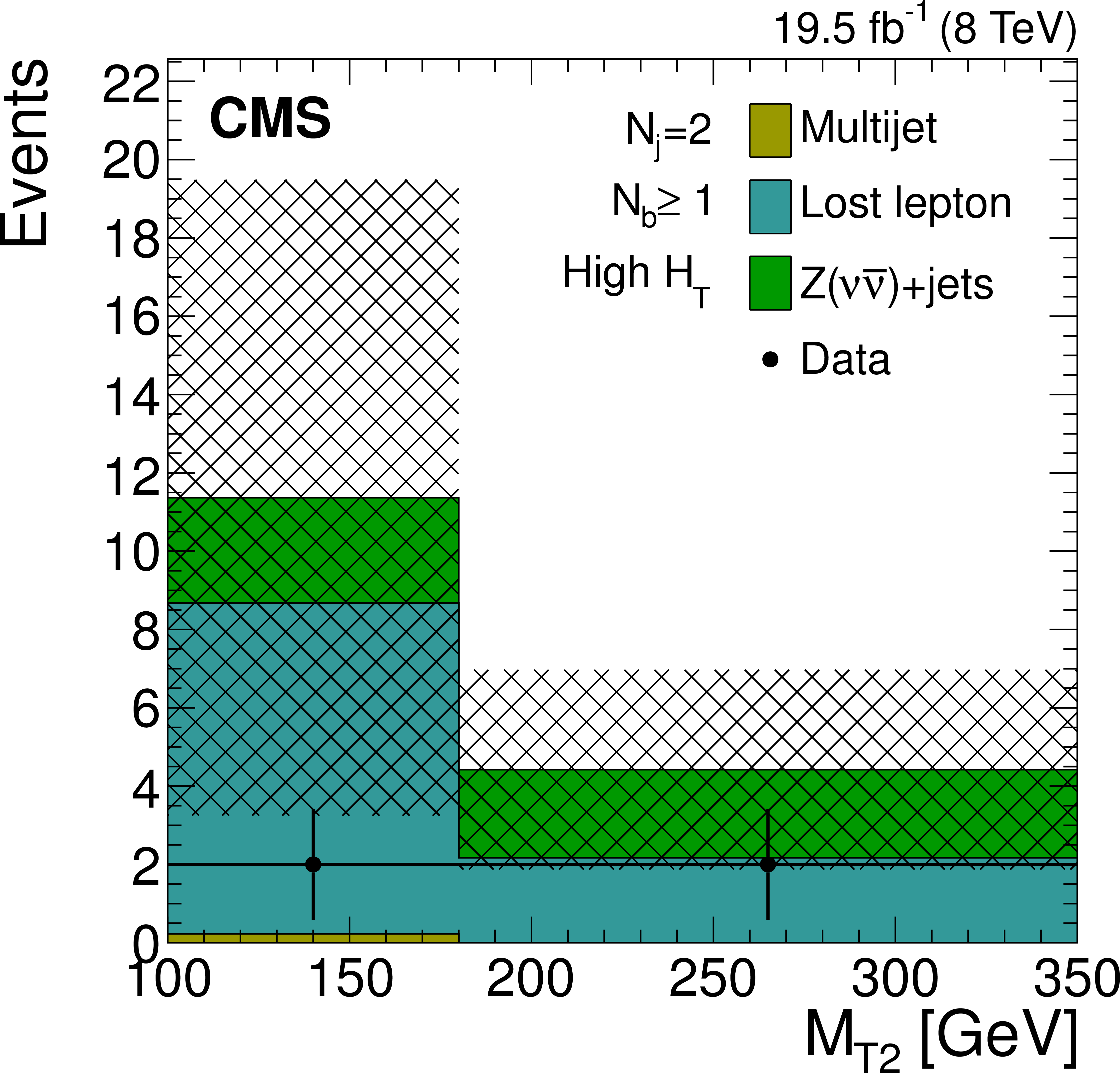
Distributions of the $ {M_{\mathrm {T2}}} $ variable for the estimated background processes and for data. Plots are shown for events satisfying the low-$ {H_{\mathrm {T}}} $ (a,d,g), the medium-$ {H_{\mathrm {T}}} $ (b,e,h), and the high-$ {H_{\mathrm {T}}} $ (c,f,i) selections, and for different topological signal regions ($ {N_\mathrm {j}} $ , $ {N_ {\mathrm {b}} } $ ) of the inclusive-$ {M_{\mathrm {T2}}} $ event selection. These are $( {N_\mathrm {j}} =2, {N_ {\mathrm {b}} } =0)$ (abs,c), $( {N_\mathrm {j}} =2, {N_ {\mathrm {b}} } \geq 1)$ (d,e,f), and $(3\leq {N_\mathrm {j}} \leq 5, {N_ {\mathrm {b}} } =0)$ (g,h,i). The uncertainties in each plot are drawn as the shaded band and do not include the uncertainty in the shape of the lost-lepton background. |
png pdf |
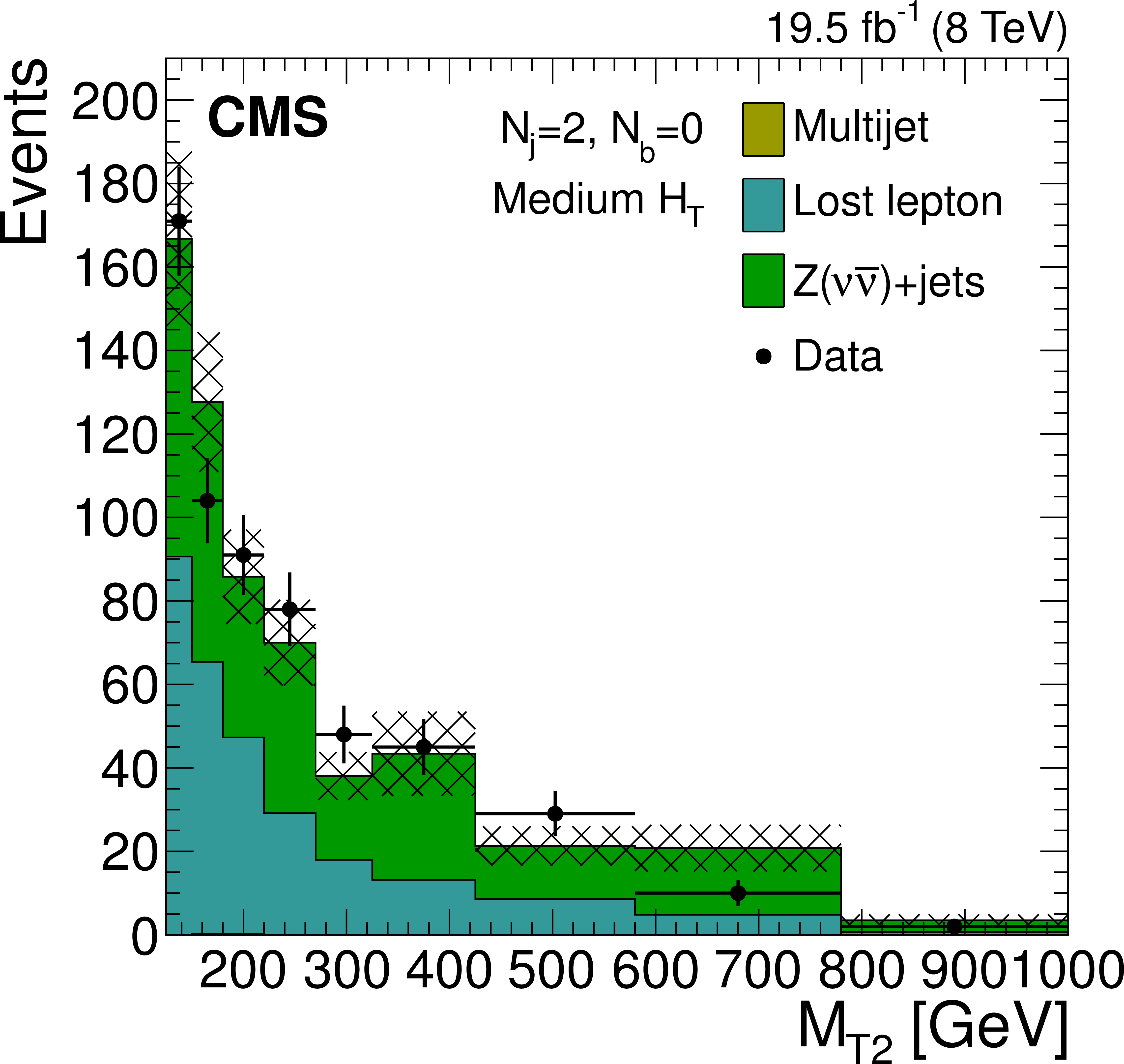
Figure 7-b:
Distributions of the $ {M_{\mathrm {T2}}} $ variable for the estimated background processes and for data. Plots are shown for events satisfying the low-$ {H_{\mathrm {T}}} $ (a,d,g), the medium-$ {H_{\mathrm {T}}} $ (b,e,h), and the high-$ {H_{\mathrm {T}}} $ (c,f,i) selections, and for different topological signal regions ($ {N_\mathrm {j}} $ , $ {N_ {\mathrm {b}} } $ ) of the inclusive-$ {M_{\mathrm {T2}}} $ event selection. These are $( {N_\mathrm {j}} =2, {N_ {\mathrm {b}} } =0)$ (abs,c), $( {N_\mathrm {j}} =2, {N_ {\mathrm {b}} } \geq 1)$ (d,e,f), and $(3\leq {N_\mathrm {j}} \leq 5, {N_ {\mathrm {b}} } =0)$ (g,h,i). The uncertainties in each plot are drawn as the shaded band and do not include the uncertainty in the shape of the lost-lepton background. |
png pdf |
Figure 7-c:
Distributions of the $ {M_{\mathrm {T2}}} $ variable for the estimated background processes and for data. Plots are shown for events satisfying the low-$ {H_{\mathrm {T}}} $ (a,d,g), the medium-$ {H_{\mathrm {T}}} $ (b,e,h), and the high-$ {H_{\mathrm {T}}} $ (c,f,i) selections, and for different topological signal regions ($ {N_\mathrm {j}} $ , $ {N_ {\mathrm {b}} } $ ) of the inclusive-$ {M_{\mathrm {T2}}} $ event selection. These are $( {N_\mathrm {j}} =2, {N_ {\mathrm {b}} } =0)$ (abs,c), $( {N_\mathrm {j}} =2, {N_ {\mathrm {b}} } \geq 1)$ (d,e,f), and $(3\leq {N_\mathrm {j}} \leq 5, {N_ {\mathrm {b}} } =0)$ (g,h,i). The uncertainties in each plot are drawn as the shaded band and do not include the uncertainty in the shape of the lost-lepton background. |
png pdf |
Figure 7-d:
Distributions of the $ {M_{\mathrm {T2}}} $ variable for the estimated background processes and for data. Plots are shown for events satisfying the low-$ {H_{\mathrm {T}}} $ (a,d,g), the medium-$ {H_{\mathrm {T}}} $ (b,e,h), and the high-$ {H_{\mathrm {T}}} $ (c,f,i) selections, and for different topological signal regions ($ {N_\mathrm {j}} $ , $ {N_ {\mathrm {b}} } $ ) of the inclusive-$ {M_{\mathrm {T2}}} $ event selection. These are $( {N_\mathrm {j}} =2, {N_ {\mathrm {b}} } =0)$ (abs,c), $( {N_\mathrm {j}} =2, {N_ {\mathrm {b}} } \geq 1)$ (d,e,f), and $(3\leq {N_\mathrm {j}} \leq 5, {N_ {\mathrm {b}} } =0)$ (g,h,i). The uncertainties in each plot are drawn as the shaded band and do not include the uncertainty in the shape of the lost-lepton background. |
png pdf |
Figure 7-e:
Distributions of the $ {M_{\mathrm {T2}}} $ variable for the estimated background processes and for data. Plots are shown for events satisfying the low-$ {H_{\mathrm {T}}} $ (a,d,g), the medium-$ {H_{\mathrm {T}}} $ (b,e,h), and the high-$ {H_{\mathrm {T}}} $ (c,f,i) selections, and for different topological signal regions ($ {N_\mathrm {j}} $ , $ {N_ {\mathrm {b}} } $ ) of the inclusive-$ {M_{\mathrm {T2}}} $ event selection. These are $( {N_\mathrm {j}} =2, {N_ {\mathrm {b}} } =0)$ (abs,c), $( {N_\mathrm {j}} =2, {N_ {\mathrm {b}} } \geq 1)$ (d,e,f), and $(3\leq {N_\mathrm {j}} \leq 5, {N_ {\mathrm {b}} } =0)$ (g,h,i). The uncertainties in each plot are drawn as the shaded band and do not include the uncertainty in the shape of the lost-lepton background. |
png pdf |
Figure 7-f:
Distributions of the $ {M_{\mathrm {T2}}} $ variable for the estimated background processes and for data. Plots are shown for events satisfying the low-$ {H_{\mathrm {T}}} $ (a,d,g), the medium-$ {H_{\mathrm {T}}} $ (b,e,h), and the high-$ {H_{\mathrm {T}}} $ (c,f,i) selections, and for different topological signal regions ($ {N_\mathrm {j}} $ , $ {N_ {\mathrm {b}} } $ ) of the inclusive-$ {M_{\mathrm {T2}}} $ event selection. These are $( {N_\mathrm {j}} =2, {N_ {\mathrm {b}} } =0)$ (abs,c), $( {N_\mathrm {j}} =2, {N_ {\mathrm {b}} } \geq 1)$ (d,e,f), and $(3\leq {N_\mathrm {j}} \leq 5, {N_ {\mathrm {b}} } =0)$ (g,h,i). The uncertainties in each plot are drawn as the shaded band and do not include the uncertainty in the shape of the lost-lepton background. |

png pdf |
Figure 7-g:
Distributions of the $ {M_{\mathrm {T2}}} $ variable for the estimated background processes and for data. Plots are shown for events satisfying the low-$ {H_{\mathrm {T}}} $ (a,d,g), the medium-$ {H_{\mathrm {T}}} $ (b,e,h), and the high-$ {H_{\mathrm {T}}} $ (c,f,i) selections, and for different topological signal regions ($ {N_\mathrm {j}} $ , $ {N_ {\mathrm {b}} } $ ) of the inclusive-$ {M_{\mathrm {T2}}} $ event selection. These are $( {N_\mathrm {j}} =2, {N_ {\mathrm {b}} } =0)$ (abs,c), $( {N_\mathrm {j}} =2, {N_ {\mathrm {b}} } \geq 1)$ (d,e,f), and $(3\leq {N_\mathrm {j}} \leq 5, {N_ {\mathrm {b}} } =0)$ (g,h,i). The uncertainties in each plot are drawn as the shaded band and do not include the uncertainty in the shape of the lost-lepton background. |
png pdf |
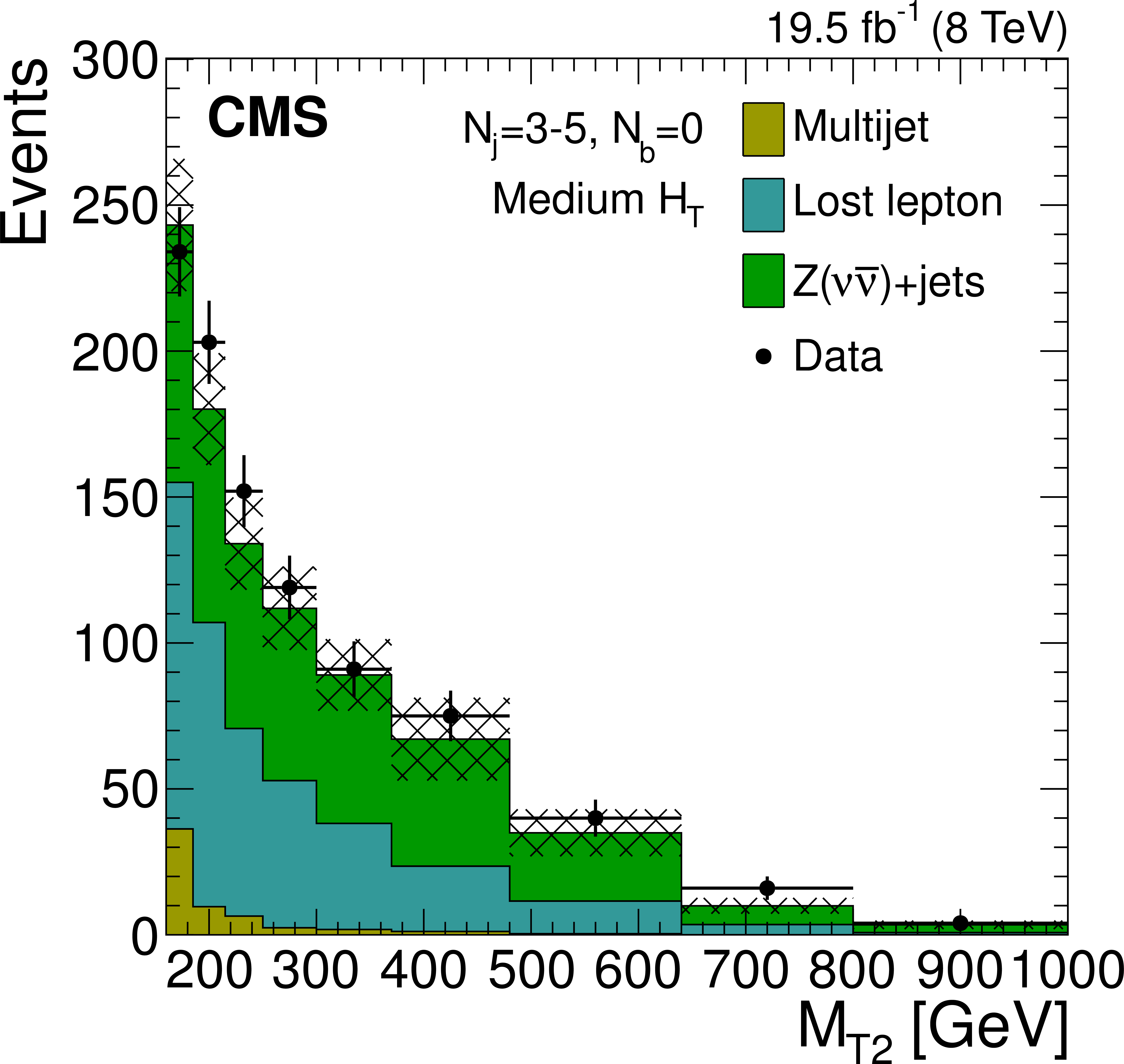
Figure 7-h:
Distributions of the $ {M_{\mathrm {T2}}} $ variable for the estimated background processes and for data. Plots are shown for events satisfying the low-$ {H_{\mathrm {T}}} $ (a,d,g), the medium-$ {H_{\mathrm {T}}} $ (b,e,h), and the high-$ {H_{\mathrm {T}}} $ (c,f,i) selections, and for different topological signal regions ($ {N_\mathrm {j}} $ , $ {N_ {\mathrm {b}} } $ ) of the inclusive-$ {M_{\mathrm {T2}}} $ event selection. These are $( {N_\mathrm {j}} =2, {N_ {\mathrm {b}} } =0)$ (abs,c), $( {N_\mathrm {j}} =2, {N_ {\mathrm {b}} } \geq 1)$ (d,e,f), and $(3\leq {N_\mathrm {j}} \leq 5, {N_ {\mathrm {b}} } =0)$ (g,h,i). The uncertainties in each plot are drawn as the shaded band and do not include the uncertainty in the shape of the lost-lepton background. |
png pdf |
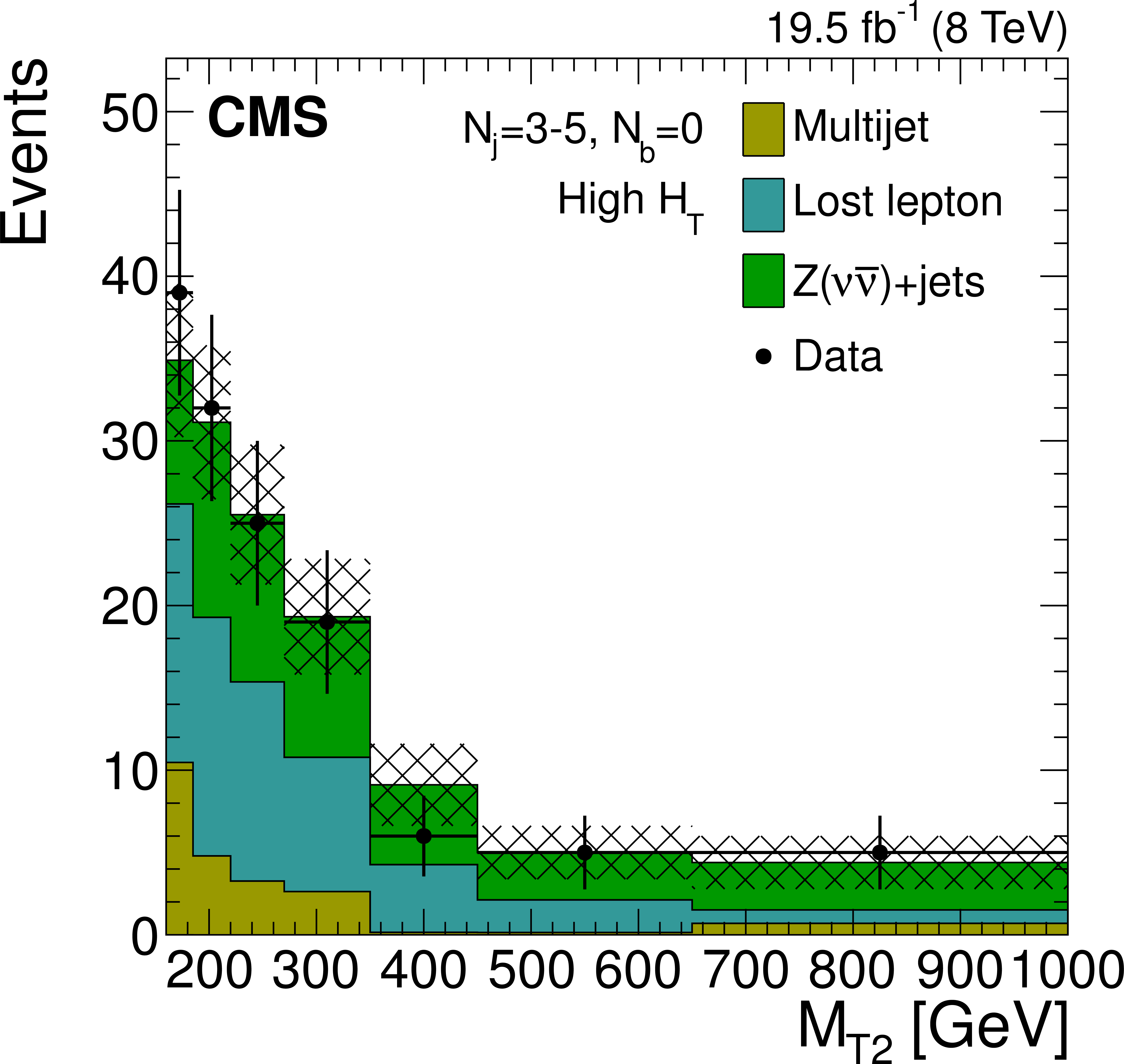
Figure 7-i:
Distributions of the $ {M_{\mathrm {T2}}} $ variable for the estimated background processes and for data. Plots are shown for events satisfying the low-$ {H_{\mathrm {T}}} $ (a,d,g), the medium-$ {H_{\mathrm {T}}} $ (b,e,h), and the high-$ {H_{\mathrm {T}}} $ (c,f,i) selections, and for different topological signal regions ($ {N_\mathrm {j}} $ , $ {N_ {\mathrm {b}} } $ ) of the inclusive-$ {M_{\mathrm {T2}}} $ event selection. These are $( {N_\mathrm {j}} =2, {N_ {\mathrm {b}} } =0)$ (abs,c), $( {N_\mathrm {j}} =2, {N_ {\mathrm {b}} } \geq 1)$ (d,e,f), and $(3\leq {N_\mathrm {j}} \leq 5, {N_ {\mathrm {b}} } =0)$ (g,h,i). The uncertainties in each plot are drawn as the shaded band and do not include the uncertainty in the shape of the lost-lepton background. |
png pdf |
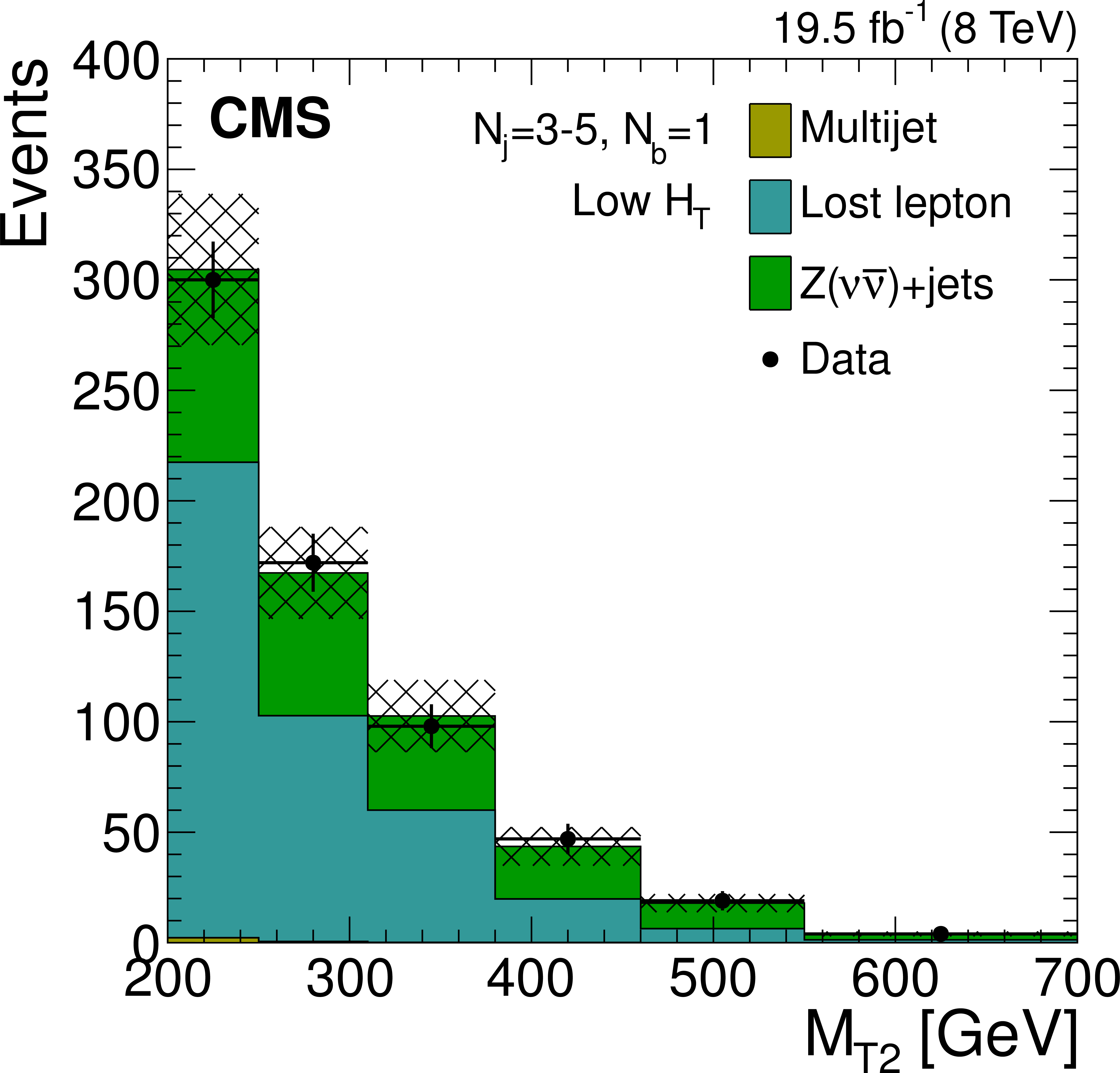
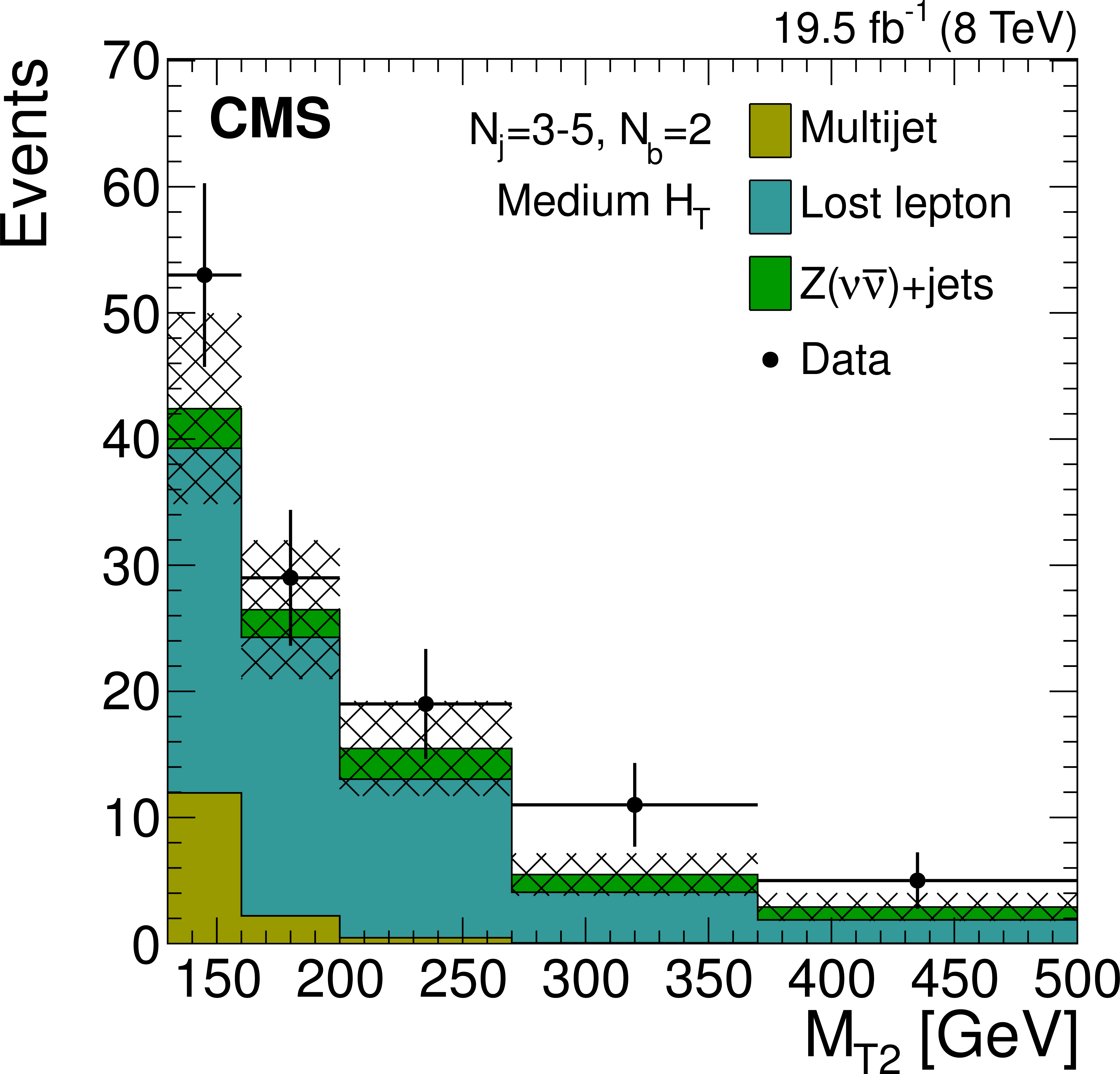
Figure 8-a:
IDistributions of the $ {M_{\mathrm {T2}}} $ variable for the estimated background processes and for data. Plots are shown for events satisfying the low-$ {H_{\mathrm {T}}} $ (a,d,g), the medium-$ {H_{\mathrm {T}}} $ (b,e,h), and the high-$ {H_{\mathrm {T}}} $ (c,f,i) selections, and for different topological signal regions ($ {N_\mathrm {j}} $ , $ {N_ {\mathrm {b}} } $ ) of the inclusive-$ {M_{\mathrm {T2}}} $ event selection. These are $(3\leq {N_\mathrm {j}} \leq 5, {N_ {\mathrm {b}} } =1)$ (a,b,c), $(3\leq {N_\mathrm {j}} \leq 5, {N_ {\mathrm {b}} } =2)$ (d,e,f), $( {N_\mathrm {j}} \geq 6, {N_ {\mathrm {b}} } =0)$ (g,h,i). The uncertainties in each plot are drawn as the shaded band and do not include the uncertainty in the shape of the lost-lepton background. |

png pdf |
Figure 8-b:
IDistributions of the $ {M_{\mathrm {T2}}} $ variable for the estimated background processes and for data. Plots are shown for events satisfying the low-$ {H_{\mathrm {T}}} $ (a,d,g), the medium-$ {H_{\mathrm {T}}} $ (b,e,h), and the high-$ {H_{\mathrm {T}}} $ (c,f,i) selections, and for different topological signal regions ($ {N_\mathrm {j}} $ , $ {N_ {\mathrm {b}} } $ ) of the inclusive-$ {M_{\mathrm {T2}}} $ event selection. These are $(3\leq {N_\mathrm {j}} \leq 5, {N_ {\mathrm {b}} } =1)$ (a,b,c), $(3\leq {N_\mathrm {j}} \leq 5, {N_ {\mathrm {b}} } =2)$ (d,e,f), $( {N_\mathrm {j}} \geq 6, {N_ {\mathrm {b}} } =0)$ (g,h,i). The uncertainties in each plot are drawn as the shaded band and do not include the uncertainty in the shape of the lost-lepton background. |
png pdf |
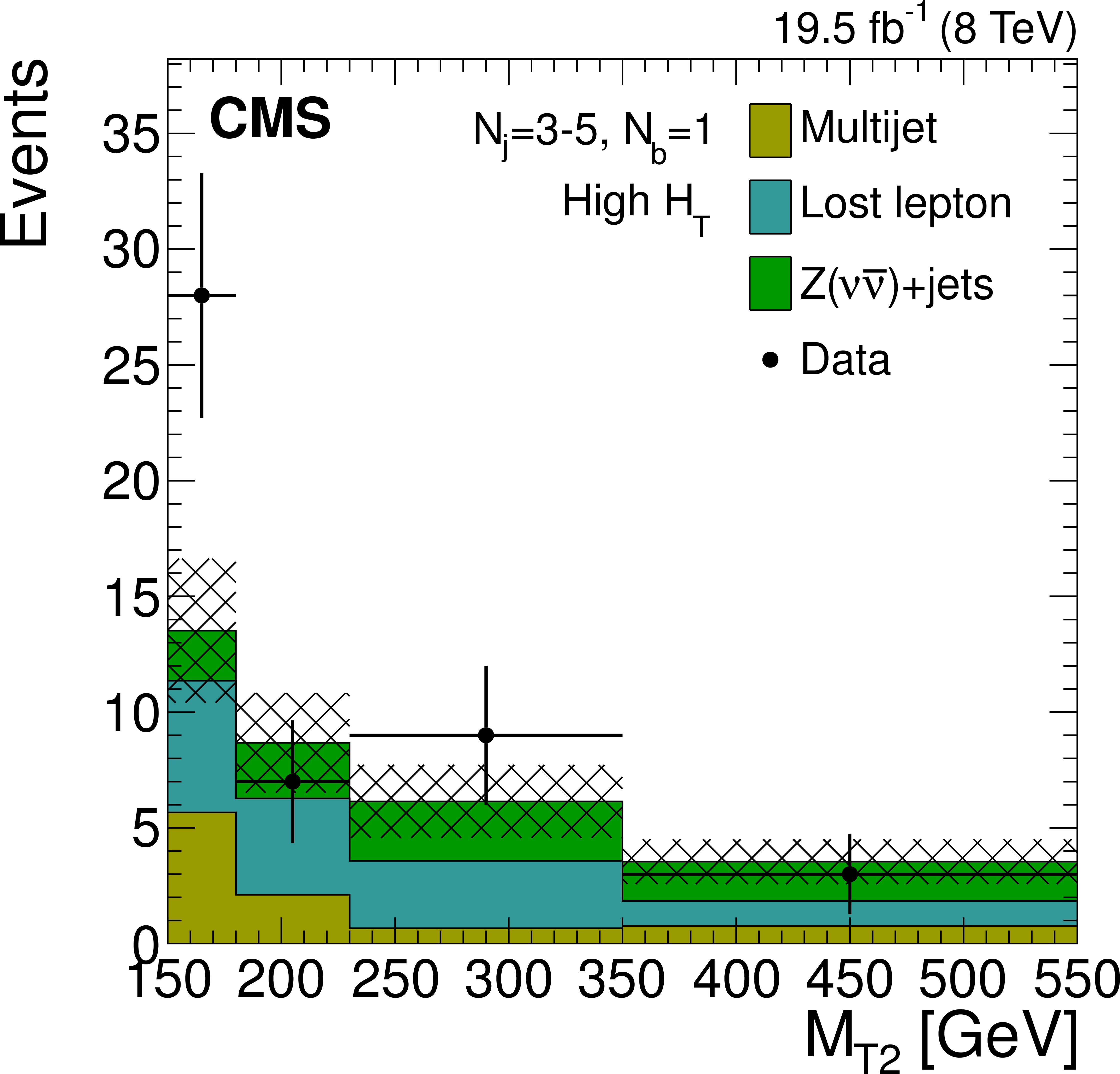
Figure 8-c:
IDistributions of the $ {M_{\mathrm {T2}}} $ variable for the estimated background processes and for data. Plots are shown for events satisfying the low-$ {H_{\mathrm {T}}} $ (a,d,g), the medium-$ {H_{\mathrm {T}}} $ (b,e,h), and the high-$ {H_{\mathrm {T}}} $ (c,f,i) selections, and for different topological signal regions ($ {N_\mathrm {j}} $ , $ {N_ {\mathrm {b}} } $ ) of the inclusive-$ {M_{\mathrm {T2}}} $ event selection. These are $(3\leq {N_\mathrm {j}} \leq 5, {N_ {\mathrm {b}} } =1)$ (a,b,c), $(3\leq {N_\mathrm {j}} \leq 5, {N_ {\mathrm {b}} } =2)$ (d,e,f), $( {N_\mathrm {j}} \geq 6, {N_ {\mathrm {b}} } =0)$ (g,h,i). The uncertainties in each plot are drawn as the shaded band and do not include the uncertainty in the shape of the lost-lepton background. |

png pdf |
Figure 8-d:
IDistributions of the $ {M_{\mathrm {T2}}} $ variable for the estimated background processes and for data. Plots are shown for events satisfying the low-$ {H_{\mathrm {T}}} $ (a,d,g), the medium-$ {H_{\mathrm {T}}} $ (b,e,h), and the high-$ {H_{\mathrm {T}}} $ (c,f,i) selections, and for different topological signal regions ($ {N_\mathrm {j}} $ , $ {N_ {\mathrm {b}} } $ ) of the inclusive-$ {M_{\mathrm {T2}}} $ event selection. These are $(3\leq {N_\mathrm {j}} \leq 5, {N_ {\mathrm {b}} } =1)$ (a,b,c), $(3\leq {N_\mathrm {j}} \leq 5, {N_ {\mathrm {b}} } =2)$ (d,e,f), $( {N_\mathrm {j}} \geq 6, {N_ {\mathrm {b}} } =0)$ (g,h,i). The uncertainties in each plot are drawn as the shaded band and do not include the uncertainty in the shape of the lost-lepton background. |
png pdf |
Figure 8-e:
IDistributions of the $ {M_{\mathrm {T2}}} $ variable for the estimated background processes and for data. Plots are shown for events satisfying the low-$ {H_{\mathrm {T}}} $ (a,d,g), the medium-$ {H_{\mathrm {T}}} $ (b,e,h), and the high-$ {H_{\mathrm {T}}} $ (c,f,i) selections, and for different topological signal regions ($ {N_\mathrm {j}} $ , $ {N_ {\mathrm {b}} } $ ) of the inclusive-$ {M_{\mathrm {T2}}} $ event selection. These are $(3\leq {N_\mathrm {j}} \leq 5, {N_ {\mathrm {b}} } =1)$ (a,b,c), $(3\leq {N_\mathrm {j}} \leq 5, {N_ {\mathrm {b}} } =2)$ (d,e,f), $( {N_\mathrm {j}} \geq 6, {N_ {\mathrm {b}} } =0)$ (g,h,i). The uncertainties in each plot are drawn as the shaded band and do not include the uncertainty in the shape of the lost-lepton background. |

png pdf |
Figure 8-f:
IDistributions of the $ {M_{\mathrm {T2}}} $ variable for the estimated background processes and for data. Plots are shown for events satisfying the low-$ {H_{\mathrm {T}}} $ (a,d,g), the medium-$ {H_{\mathrm {T}}} $ (b,e,h), and the high-$ {H_{\mathrm {T}}} $ (c,f,i) selections, and for different topological signal regions ($ {N_\mathrm {j}} $ , $ {N_ {\mathrm {b}} } $ ) of the inclusive-$ {M_{\mathrm {T2}}} $ event selection. These are $(3\leq {N_\mathrm {j}} \leq 5, {N_ {\mathrm {b}} } =1)$ (a,b,c), $(3\leq {N_\mathrm {j}} \leq 5, {N_ {\mathrm {b}} } =2)$ (d,e,f), $( {N_\mathrm {j}} \geq 6, {N_ {\mathrm {b}} } =0)$ (g,h,i). The uncertainties in each plot are drawn as the shaded band and do not include the uncertainty in the shape of the lost-lepton background. |
png pdf |
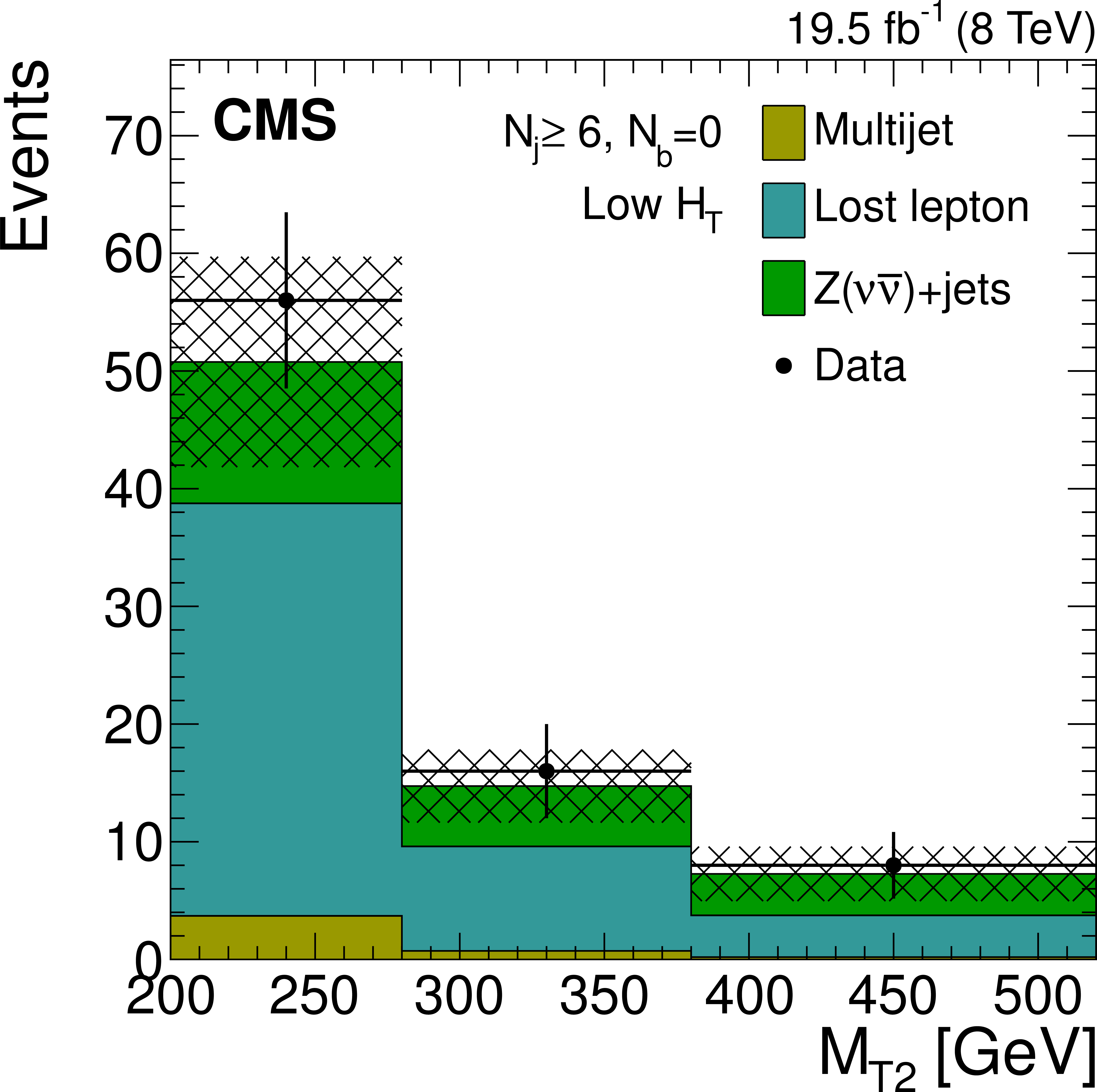
Figure 8-g:
IDistributions of the $ {M_{\mathrm {T2}}} $ variable for the estimated background processes and for data. Plots are shown for events satisfying the low-$ {H_{\mathrm {T}}} $ (a,d,g), the medium-$ {H_{\mathrm {T}}} $ (b,e,h), and the high-$ {H_{\mathrm {T}}} $ (c,f,i) selections, and for different topological signal regions ($ {N_\mathrm {j}} $ , $ {N_ {\mathrm {b}} } $ ) of the inclusive-$ {M_{\mathrm {T2}}} $ event selection. These are $(3\leq {N_\mathrm {j}} \leq 5, {N_ {\mathrm {b}} } =1)$ (a,b,c), $(3\leq {N_\mathrm {j}} \leq 5, {N_ {\mathrm {b}} } =2)$ (d,e,f), $( {N_\mathrm {j}} \geq 6, {N_ {\mathrm {b}} } =0)$ (g,h,i). The uncertainties in each plot are drawn as the shaded band and do not include the uncertainty in the shape of the lost-lepton background. |
png pdf |
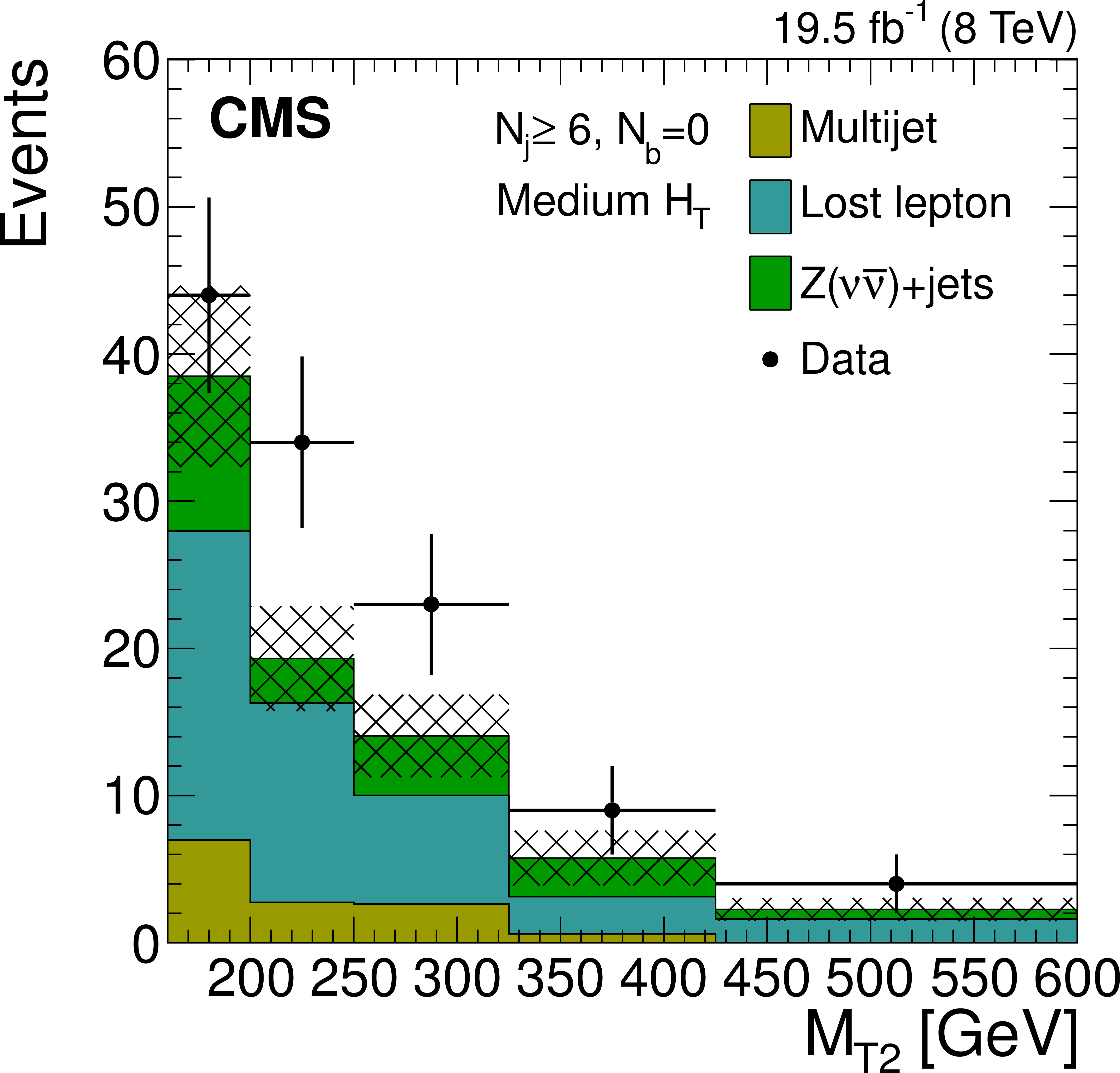
Figure 8-h:
IDistributions of the $ {M_{\mathrm {T2}}} $ variable for the estimated background processes and for data. Plots are shown for events satisfying the low-$ {H_{\mathrm {T}}} $ (a,d,g), the medium-$ {H_{\mathrm {T}}} $ (b,e,h), and the high-$ {H_{\mathrm {T}}} $ (c,f,i) selections, and for different topological signal regions ($ {N_\mathrm {j}} $ , $ {N_ {\mathrm {b}} } $ ) of the inclusive-$ {M_{\mathrm {T2}}} $ event selection. These are $(3\leq {N_\mathrm {j}} \leq 5, {N_ {\mathrm {b}} } =1)$ (a,b,c), $(3\leq {N_\mathrm {j}} \leq 5, {N_ {\mathrm {b}} } =2)$ (d,e,f), $( {N_\mathrm {j}} \geq 6, {N_ {\mathrm {b}} } =0)$ (g,h,i). The uncertainties in each plot are drawn as the shaded band and do not include the uncertainty in the shape of the lost-lepton background. |

png pdf |
Figure 8-i:
IDistributions of the $ {M_{\mathrm {T2}}} $ variable for the estimated background processes and for data. Plots are shown for events satisfying the low-$ {H_{\mathrm {T}}} $ (a,d,g), the medium-$ {H_{\mathrm {T}}} $ (b,e,h), and the high-$ {H_{\mathrm {T}}} $ (c,f,i) selections, and for different topological signal regions ($ {N_\mathrm {j}} $ , $ {N_ {\mathrm {b}} } $ ) of the inclusive-$ {M_{\mathrm {T2}}} $ event selection. These are $(3\leq {N_\mathrm {j}} \leq 5, {N_ {\mathrm {b}} } =1)$ (a,b,c), $(3\leq {N_\mathrm {j}} \leq 5, {N_ {\mathrm {b}} } =2)$ (d,e,f), $( {N_\mathrm {j}} \geq 6, {N_ {\mathrm {b}} } =0)$ (g,h,i). The uncertainties in each plot are drawn as the shaded band and do not include the uncertainty in the shape of the lost-lepton background. |
png pdf |
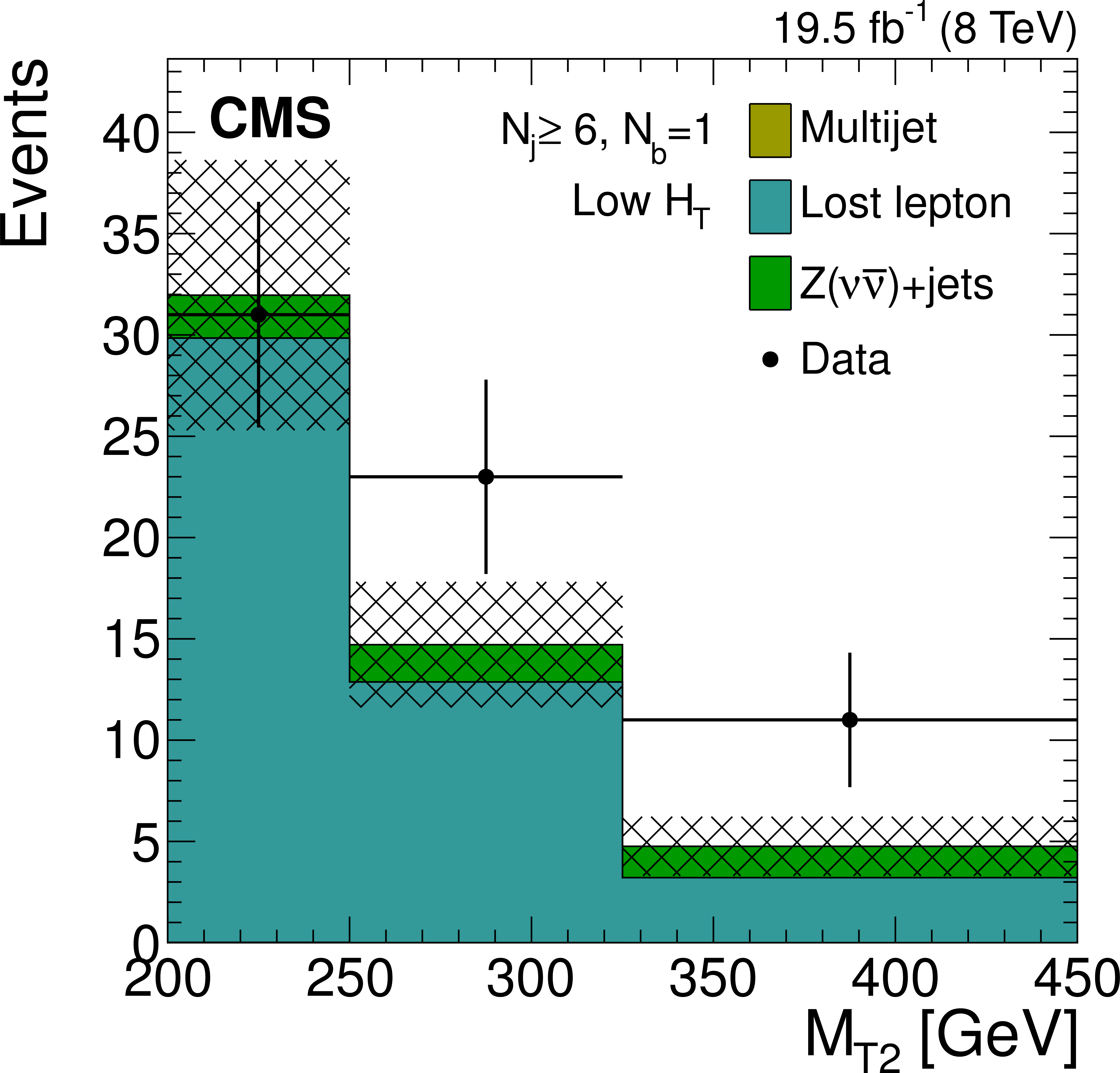
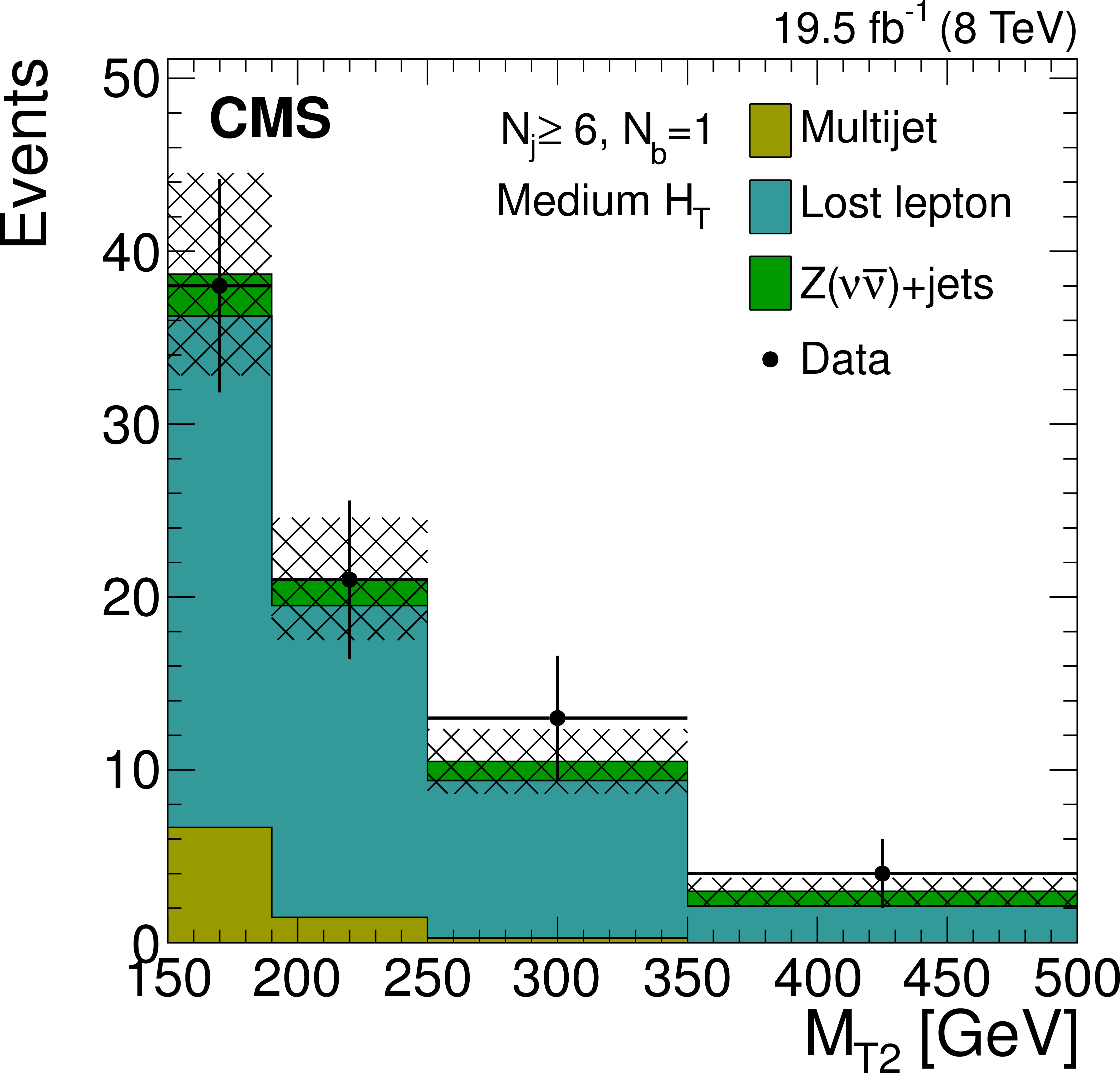
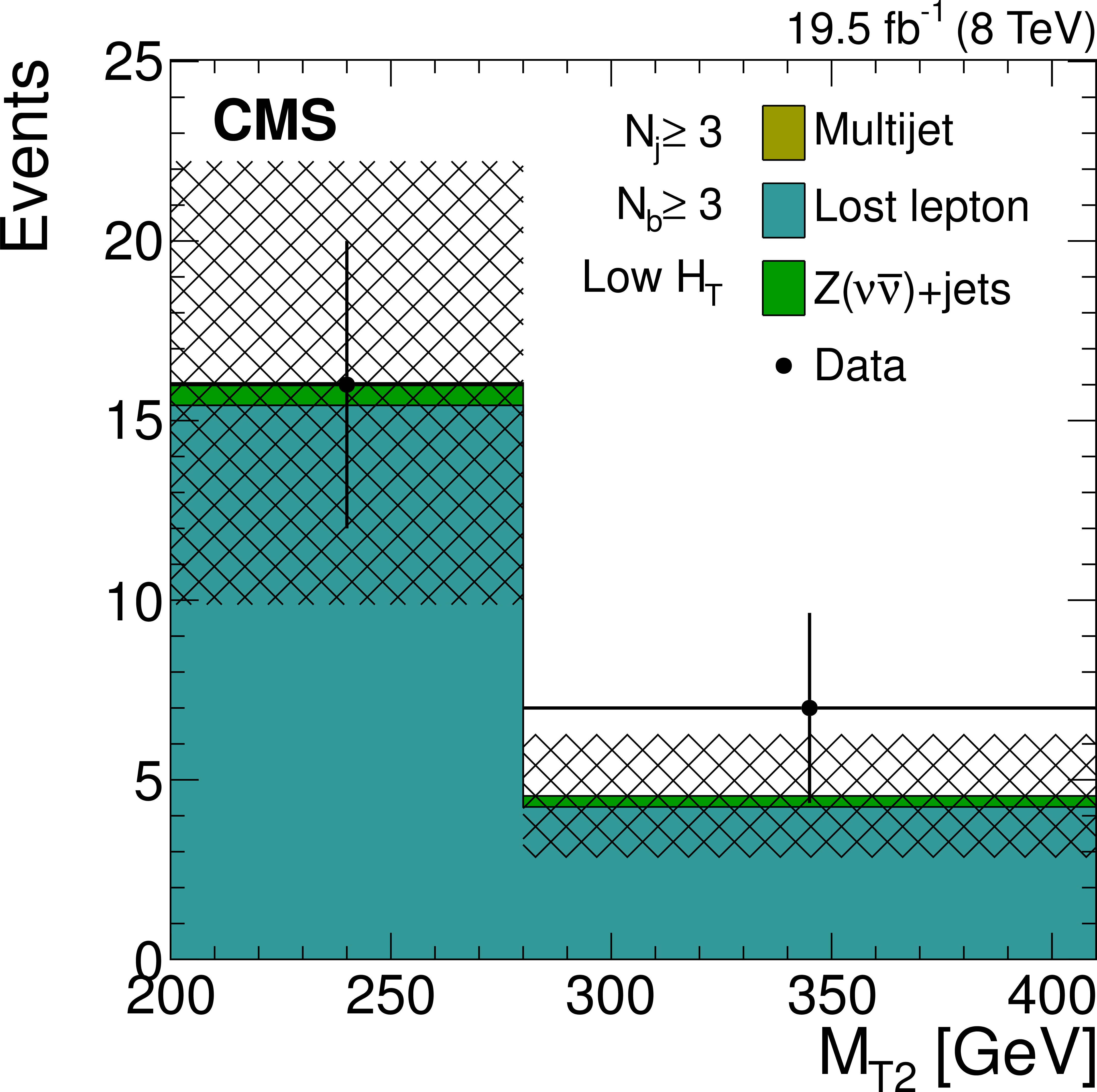
Figure 9-a:
Distributions of the $ {M_{\mathrm {T2}}} $ variable for the estimated background processes and for data. Plots are shown for events satisfying the low-$ {H_{\mathrm {T}}} $ (a,d,g), the medium-$ {H_{\mathrm {T}}} $ (b,e,h), and the high-$ {H_{\mathrm {T}}} $ (c,f,i) selections, and for different topological signal regions ($ {N_\mathrm {j}} $ , $ {N_ {\mathrm {b}} } $ ) of the inclusive-$ {M_{\mathrm {T2}}} $ event selection. These are $( {N_\mathrm {j}} \geq 6, {N_ {\mathrm {b}} } =1)$ (a,b,c), $( {N_\mathrm {j}} \geq 6, {N_ {\mathrm {b}} } =2)$ (d,e,f), $( {N_\mathrm {j}} \geq 3, {N_ {\mathrm {b}} } \geq 3)$ (g,h,i). The uncertainties in each plot are drawn as the shaded band and do not include the uncertainty in the shape of the lost-lepton background. |
png pdf |
Figure 9-b:
Distributions of the $ {M_{\mathrm {T2}}} $ variable for the estimated background processes and for data. Plots are shown for events satisfying the low-$ {H_{\mathrm {T}}} $ (a,d,g), the medium-$ {H_{\mathrm {T}}} $ (b,e,h), and the high-$ {H_{\mathrm {T}}} $ (c,f,i) selections, and for different topological signal regions ($ {N_\mathrm {j}} $ , $ {N_ {\mathrm {b}} } $ ) of the inclusive-$ {M_{\mathrm {T2}}} $ event selection. These are $( {N_\mathrm {j}} \geq 6, {N_ {\mathrm {b}} } =1)$ (a,b,c), $( {N_\mathrm {j}} \geq 6, {N_ {\mathrm {b}} } =2)$ (d,e,f), $( {N_\mathrm {j}} \geq 3, {N_ {\mathrm {b}} } \geq 3)$ (g,h,i). The uncertainties in each plot are drawn as the shaded band and do not include the uncertainty in the shape of the lost-lepton background. |

png pdf |
Figure 9-c:
Distributions of the $ {M_{\mathrm {T2}}} $ variable for the estimated background processes and for data. Plots are shown for events satisfying the low-$ {H_{\mathrm {T}}} $ (a,d,g), the medium-$ {H_{\mathrm {T}}} $ (b,e,h), and the high-$ {H_{\mathrm {T}}} $ (c,f,i) selections, and for different topological signal regions ($ {N_\mathrm {j}} $ , $ {N_ {\mathrm {b}} } $ ) of the inclusive-$ {M_{\mathrm {T2}}} $ event selection. These are $( {N_\mathrm {j}} \geq 6, {N_ {\mathrm {b}} } =1)$ (a,b,c), $( {N_\mathrm {j}} \geq 6, {N_ {\mathrm {b}} } =2)$ (d,e,f), $( {N_\mathrm {j}} \geq 3, {N_ {\mathrm {b}} } \geq 3)$ (g,h,i). The uncertainties in each plot are drawn as the shaded band and do not include the uncertainty in the shape of the lost-lepton background. |
png pdf |
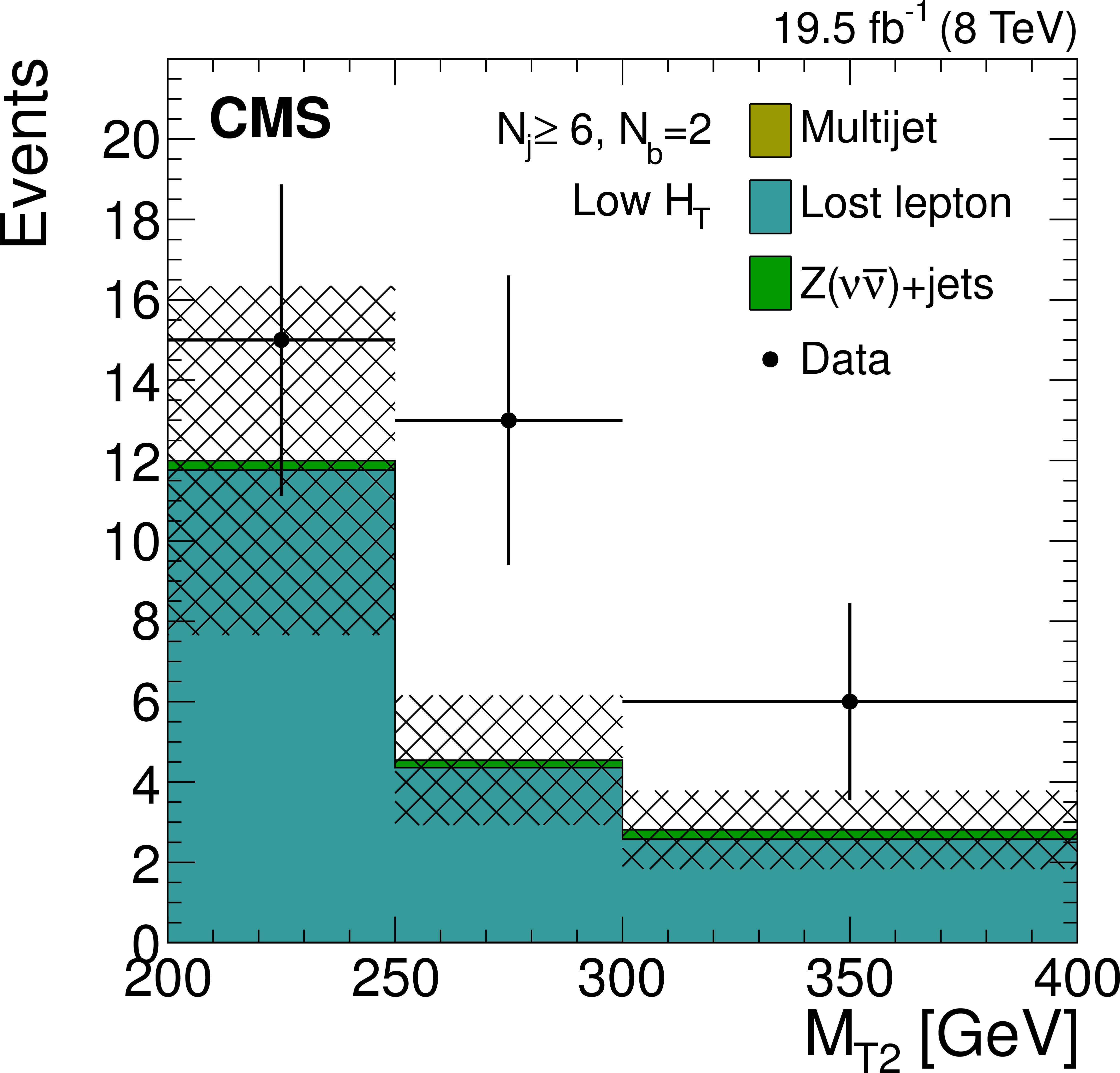
Figure 9-d:
Distributions of the $ {M_{\mathrm {T2}}} $ variable for the estimated background processes and for data. Plots are shown for events satisfying the low-$ {H_{\mathrm {T}}} $ (a,d,g), the medium-$ {H_{\mathrm {T}}} $ (b,e,h), and the high-$ {H_{\mathrm {T}}} $ (c,f,i) selections, and for different topological signal regions ($ {N_\mathrm {j}} $ , $ {N_ {\mathrm {b}} } $ ) of the inclusive-$ {M_{\mathrm {T2}}} $ event selection. These are $( {N_\mathrm {j}} \geq 6, {N_ {\mathrm {b}} } =1)$ (a,b,c), $( {N_\mathrm {j}} \geq 6, {N_ {\mathrm {b}} } =2)$ (d,e,f), $( {N_\mathrm {j}} \geq 3, {N_ {\mathrm {b}} } \geq 3)$ (g,h,i). The uncertainties in each plot are drawn as the shaded band and do not include the uncertainty in the shape of the lost-lepton background. |
png pdf |
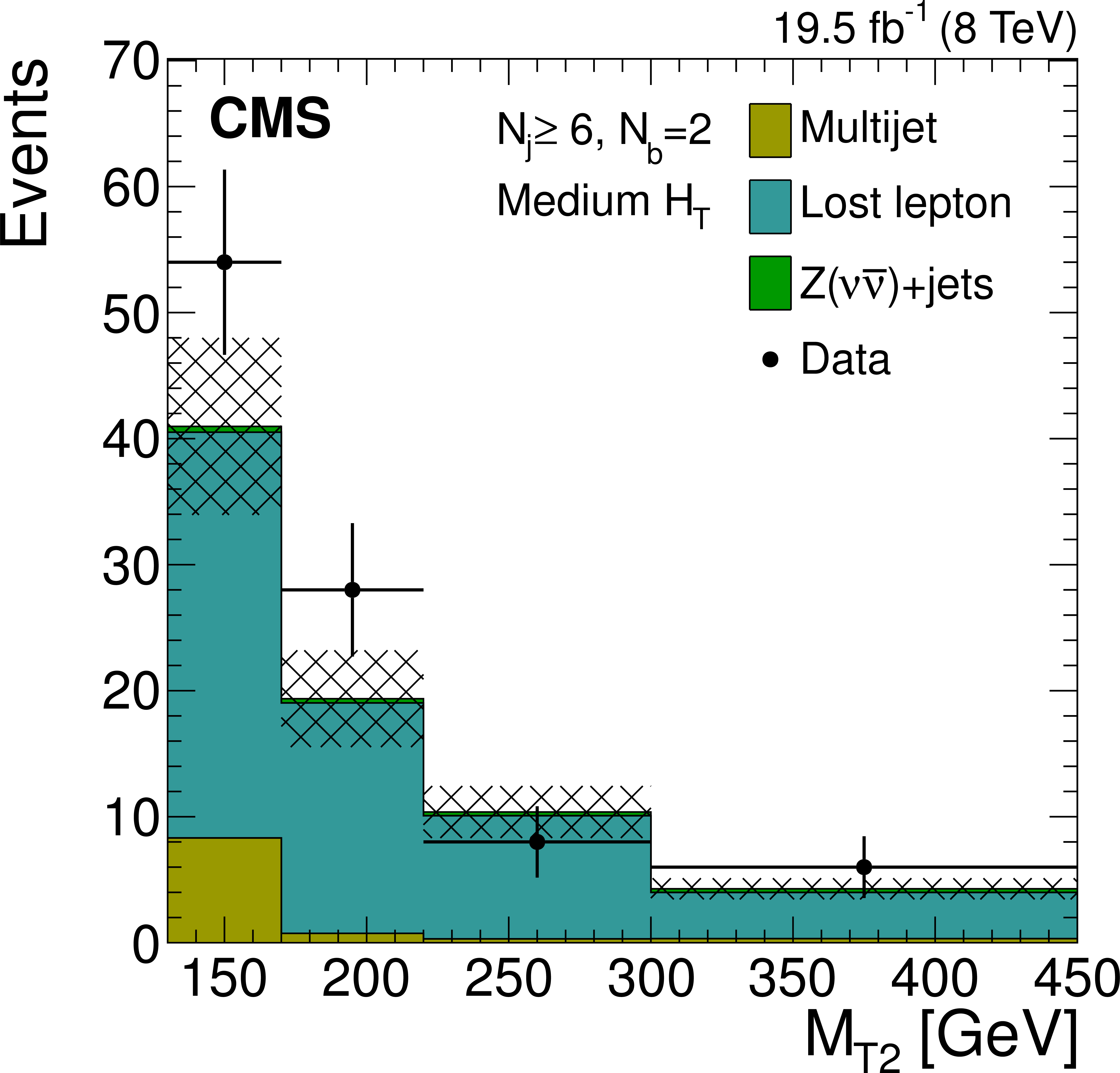
Figure 9-e:
Distributions of the $ {M_{\mathrm {T2}}} $ variable for the estimated background processes and for data. Plots are shown for events satisfying the low-$ {H_{\mathrm {T}}} $ (a,d,g), the medium-$ {H_{\mathrm {T}}} $ (b,e,h), and the high-$ {H_{\mathrm {T}}} $ (c,f,i) selections, and for different topological signal regions ($ {N_\mathrm {j}} $ , $ {N_ {\mathrm {b}} } $ ) of the inclusive-$ {M_{\mathrm {T2}}} $ event selection. These are $( {N_\mathrm {j}} \geq 6, {N_ {\mathrm {b}} } =1)$ (a,b,c), $( {N_\mathrm {j}} \geq 6, {N_ {\mathrm {b}} } =2)$ (d,e,f), $( {N_\mathrm {j}} \geq 3, {N_ {\mathrm {b}} } \geq 3)$ (g,h,i). The uncertainties in each plot are drawn as the shaded band and do not include the uncertainty in the shape of the lost-lepton background. |
png pdf |
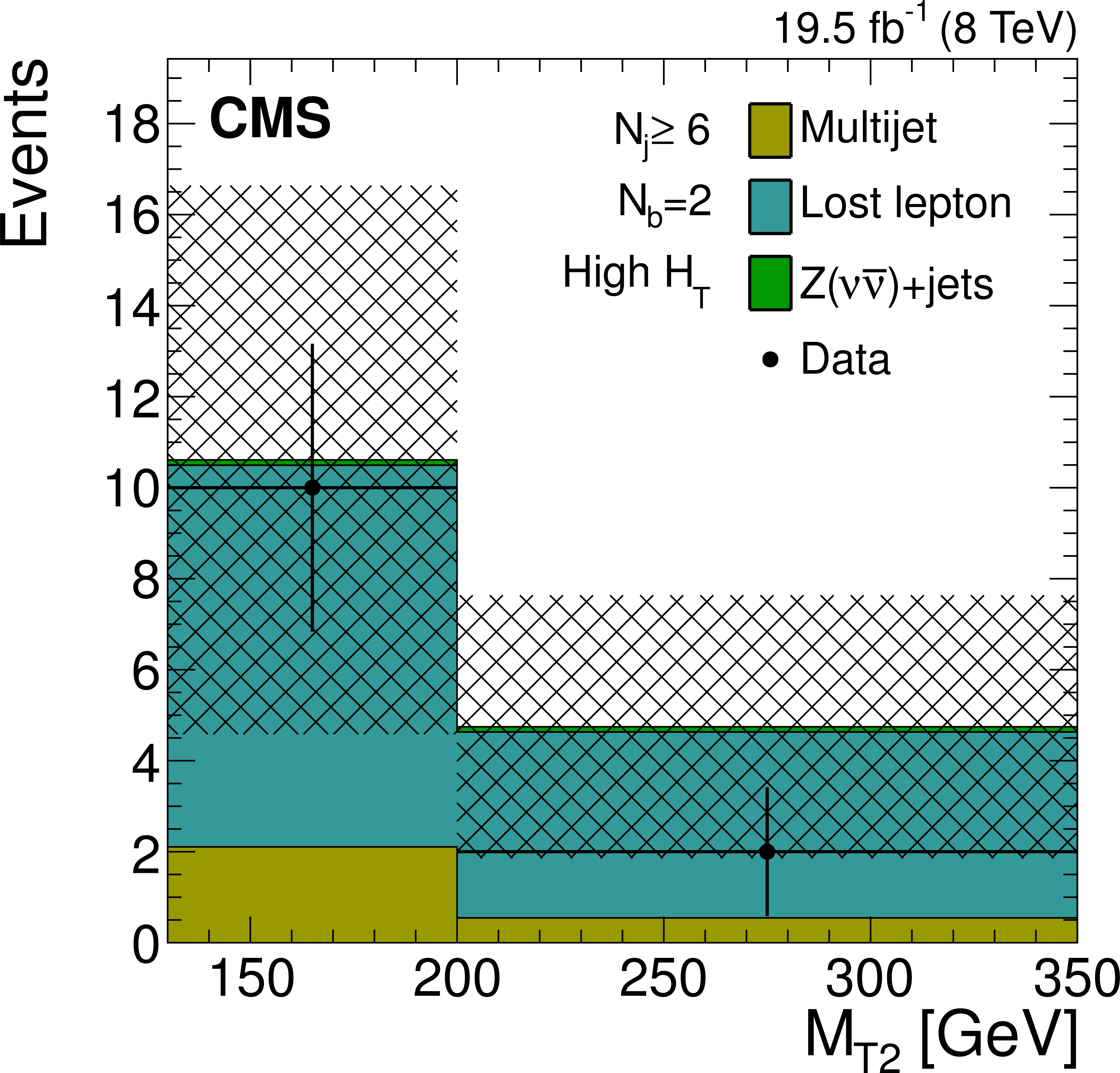
Figure 9-f:
Distributions of the $ {M_{\mathrm {T2}}} $ variable for the estimated background processes and for data. Plots are shown for events satisfying the low-$ {H_{\mathrm {T}}} $ (a,d,g), the medium-$ {H_{\mathrm {T}}} $ (b,e,h), and the high-$ {H_{\mathrm {T}}} $ (c,f,i) selections, and for different topological signal regions ($ {N_\mathrm {j}} $ , $ {N_ {\mathrm {b}} } $ ) of the inclusive-$ {M_{\mathrm {T2}}} $ event selection. These are $( {N_\mathrm {j}} \geq 6, {N_ {\mathrm {b}} } =1)$ (a,b,c), $( {N_\mathrm {j}} \geq 6, {N_ {\mathrm {b}} } =2)$ (d,e,f), $( {N_\mathrm {j}} \geq 3, {N_ {\mathrm {b}} } \geq 3)$ (g,h,i). The uncertainties in each plot are drawn as the shaded band and do not include the uncertainty in the shape of the lost-lepton background. |
png pdf |
Figure 9-g:
Distributions of the $ {M_{\mathrm {T2}}} $ variable for the estimated background processes and for data. Plots are shown for events satisfying the low-$ {H_{\mathrm {T}}} $ (a,d,g), the medium-$ {H_{\mathrm {T}}} $ (b,e,h), and the high-$ {H_{\mathrm {T}}} $ (c,f,i) selections, and for different topological signal regions ($ {N_\mathrm {j}} $ , $ {N_ {\mathrm {b}} } $ ) of the inclusive-$ {M_{\mathrm {T2}}} $ event selection. These are $( {N_\mathrm {j}} \geq 6, {N_ {\mathrm {b}} } =1)$ (a,b,c), $( {N_\mathrm {j}} \geq 6, {N_ {\mathrm {b}} } =2)$ (d,e,f), $( {N_\mathrm {j}} \geq 3, {N_ {\mathrm {b}} } \geq 3)$ (g,h,i). The uncertainties in each plot are drawn as the shaded band and do not include the uncertainty in the shape of the lost-lepton background. |
png pdf |
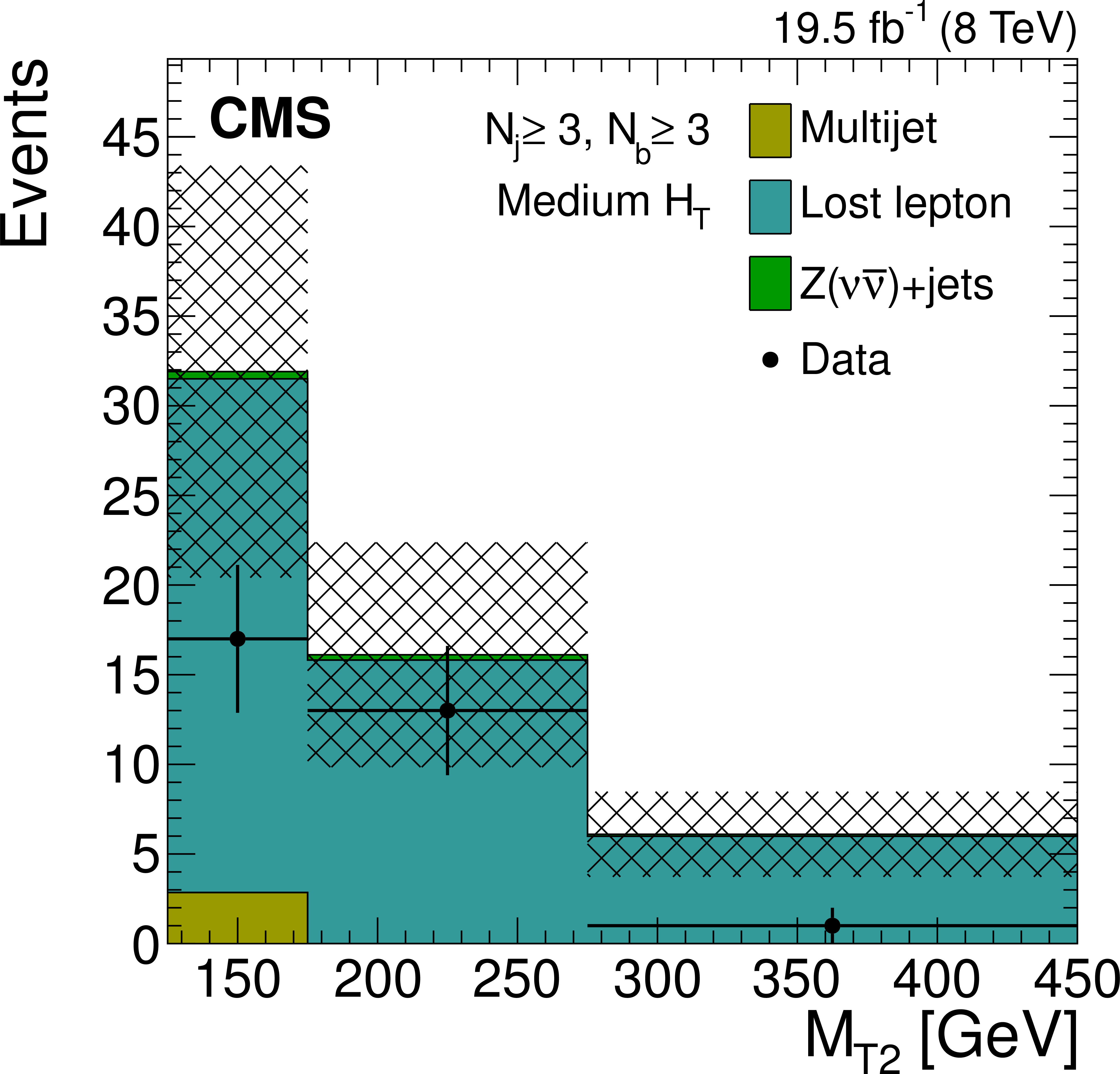
Figure 9-h:
Distributions of the $ {M_{\mathrm {T2}}} $ variable for the estimated background processes and for data. Plots are shown for events satisfying the low-$ {H_{\mathrm {T}}} $ (a,d,g), the medium-$ {H_{\mathrm {T}}} $ (b,e,h), and the high-$ {H_{\mathrm {T}}} $ (c,f,i) selections, and for different topological signal regions ($ {N_\mathrm {j}} $ , $ {N_ {\mathrm {b}} } $ ) of the inclusive-$ {M_{\mathrm {T2}}} $ event selection. These are $( {N_\mathrm {j}} \geq 6, {N_ {\mathrm {b}} } =1)$ (a,b,c), $( {N_\mathrm {j}} \geq 6, {N_ {\mathrm {b}} } =2)$ (d,e,f), $( {N_\mathrm {j}} \geq 3, {N_ {\mathrm {b}} } \geq 3)$ (g,h,i). The uncertainties in each plot are drawn as the shaded band and do not include the uncertainty in the shape of the lost-lepton background. |
png pdf |
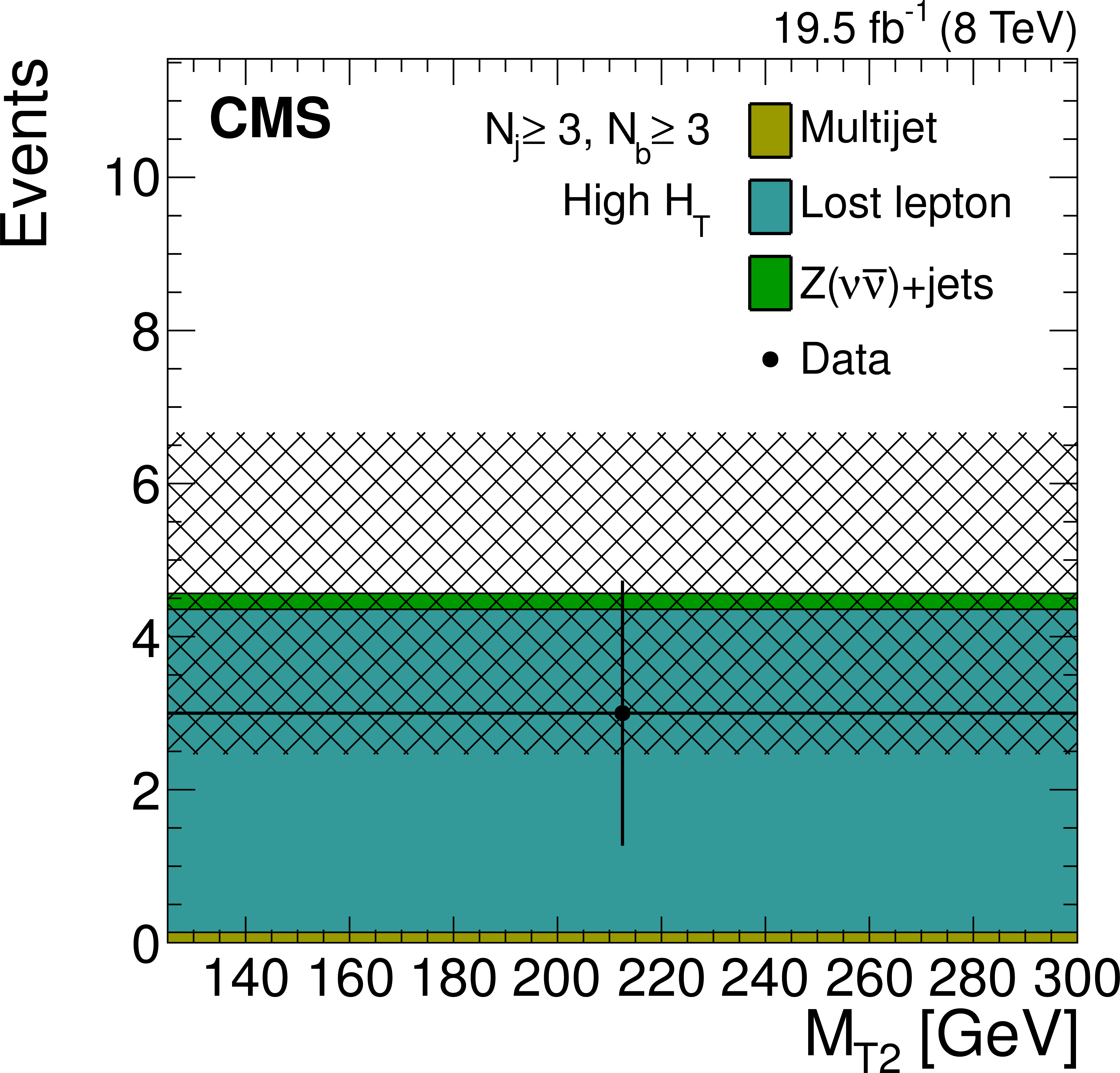
Figure 9-i:
Distributions of the $ {M_{\mathrm {T2}}} $ variable for the estimated background processes and for data. Plots are shown for events satisfying the low-$ {H_{\mathrm {T}}} $ (a,d,g), the medium-$ {H_{\mathrm {T}}} $ (b,e,h), and the high-$ {H_{\mathrm {T}}} $ (c,f,i) selections, and for different topological signal regions ($ {N_\mathrm {j}} $ , $ {N_ {\mathrm {b}} } $ ) of the inclusive-$ {M_{\mathrm {T2}}} $ event selection. These are $( {N_\mathrm {j}} \geq 6, {N_ {\mathrm {b}} } =1)$ (a,b,c), $( {N_\mathrm {j}} \geq 6, {N_ {\mathrm {b}} } =2)$ (d,e,f), $( {N_\mathrm {j}} \geq 3, {N_ {\mathrm {b}} } \geq 3)$ (g,h,i). The uncertainties in each plot are drawn as the shaded band and do not include the uncertainty in the shape of the lost-lepton background. |

png pdf |
Figure 10:
Event yields, for both estimated backgrounds and data, for the three $ {H_{\mathrm {T}}} $ selections and all the topological signal regions of the inclusive-$ {M_{\mathrm {T2}}} $ search. The uncertainties are drawn as the shaded band and do not include the uncertainty in the shape of the lost-lepton background. |
png pdf |
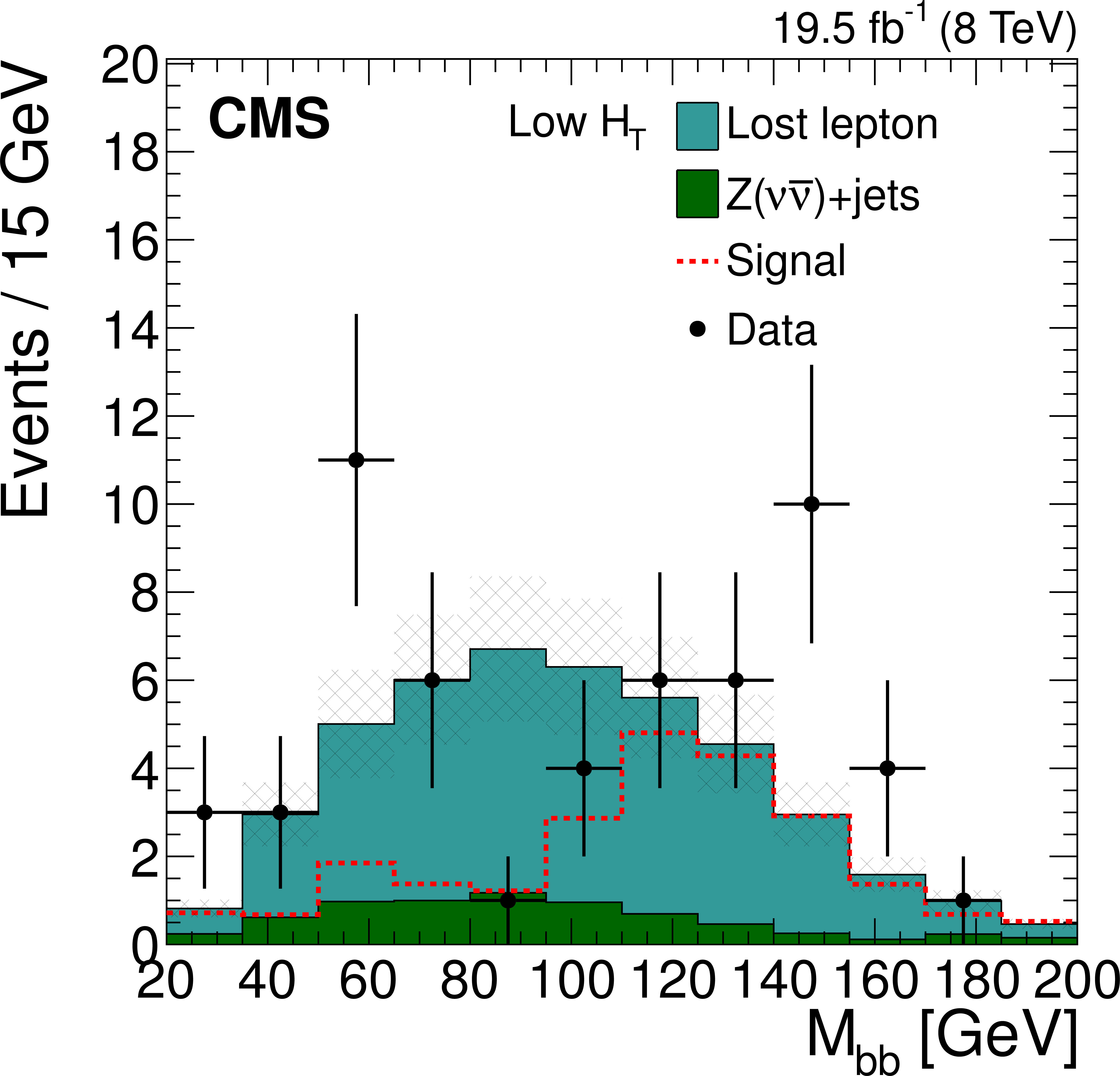
Figure 11-a:
Distributions of the $ {M_{ {\mathrm {b}} {\mathrm {b}} }} $ variable for the $ {\mathrm {W}}( {\ell \nu })$+jets and $ {\mathrm {t}\overline {\mathrm {t}}} $+jets processes (i.e. the lost-lepton background), the $ {\mathrm {Z}} ( {\nu {\overline {\nu }} })$+jets background, data, and a possible SUSY signal. The distributions are shown for both the low- (a) and the high-$ {H_{\mathrm {T}}} $ (b) selections of the $ {M_{\mathrm {T2}}} $-Higgs search. The lost-lepton background is estimated from data control samples, while the $ {\mathrm {Z}} ( {\nu {\overline {\nu }} })$+jets is evaluated using simulation. The uncertainties in each plot are drawn as the shaded band and do not include the uncertainty in the shape of the lost-lepton background. The signal model consists of gluino pair production events with one of the two gluinos containing an h boson in its decay chain. For this model it is assumed $ m_{ {\mathrm{ \tilde{g} } } } = 750 $ GeV and $ m_{ {\tilde{\chi}^{0}_{1}} } = 350 $ GeV. |

png pdf |
Figure 11-b:
Distributions of the $ {M_{ {\mathrm {b}} {\mathrm {b}} }} $ variable for the $ {\mathrm {W}}( {\ell \nu })$+jets and $ {\mathrm {t}\overline {\mathrm {t}}} $+jets processes (i.e. the lost-lepton background), the $ {\mathrm {Z}} ( {\nu {\overline {\nu }} })$+jets background, data, and a possible SUSY signal. The distributions are shown for both the low- (a) and the high-$ {H_{\mathrm {T}}} $ (b) selections of the $ {M_{\mathrm {T2}}} $-Higgs search. The lost-lepton background is estimated from data control samples, while the $ {\mathrm {Z}} ( {\nu {\overline {\nu }} })$+jets is evaluated using simulation. The uncertainties in each plot are drawn as the shaded band and do not include the uncertainty in the shape of the lost-lepton background. The signal model consists of gluino pair production events with one of the two gluinos containing an h boson in its decay chain. For this model it is assumed $ m_{ {\mathrm{ \tilde{g} } } } = 750 $ GeV and $ m_{ {\tilde{\chi}^{0}_{1}} } = 350 $ GeV. |

png pdf |
Figure 12-a:
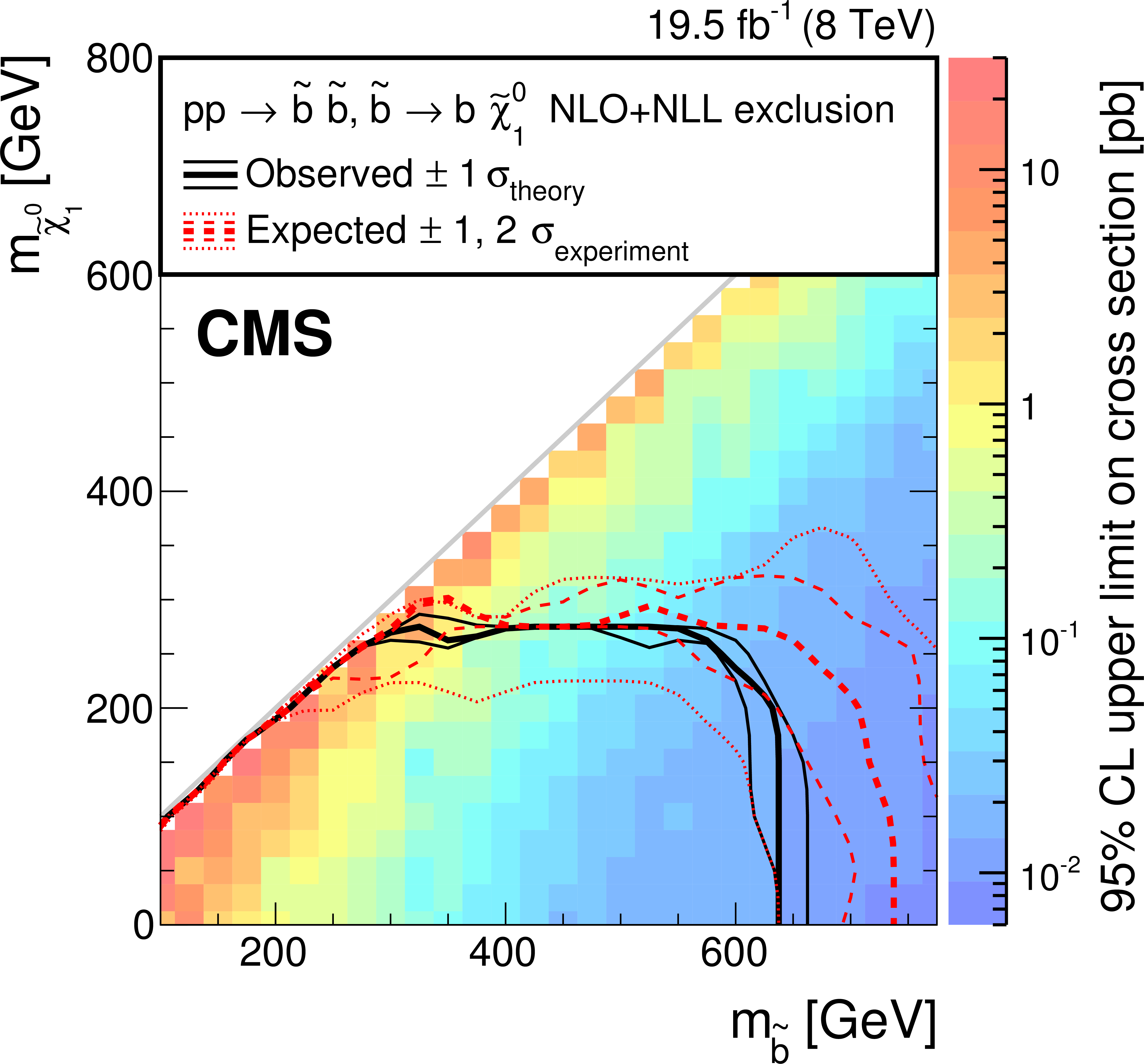
5Exclusion limits at 95% CL for (upper left) direct squark production, (upper right) direct bottom-squark production, and (bottom) direct top-squark production. For the direct squark production, the upper set of curves corresponds to the scenario where the first two generations of squarks are degenerate and light, while the lower set corresponds to only one accessible light-flavour squark. For convenience, diagonal lines have been drawn corresponding to $ m_{ {\tilde{\chi}^{0}_{1}} } = m_{ \mathrm{ \tilde{q}, \tilde{b}, \tilde{t} } }$ and $ {m_{ {\tilde{\chi}^{0}_{1}} }} =m_{ \mathrm{ \tilde{q}, \tilde{b}, \tilde{t} } } - \left (m_{ {\mathrm {W}}} + {m_{ {\mathrm {b}} }} \right )$ where applicable. |
png pdf |
Figure 12-b:
5Exclusion limits at 95% CL for (upper left) direct squark production, (upper right) direct bottom-squark production, and (bottom) direct top-squark production. For the direct squark production, the upper set of curves corresponds to the scenario where the first two generations of squarks are degenerate and light, while the lower set corresponds to only one accessible light-flavour squark. For convenience, diagonal lines have been drawn corresponding to $ m_{ {\tilde{\chi}^{0}_{1}} } = m_{ \mathrm{ \tilde{q}, \tilde{b}, \tilde{t} } }$ and $ {m_{ {\tilde{\chi}^{0}_{1}} }} =m_{ \mathrm{ \tilde{q}, \tilde{b}, \tilde{t} } } - \left (m_{ {\mathrm {W}}} + {m_{ {\mathrm {b}} }} \right )$ where applicable. |
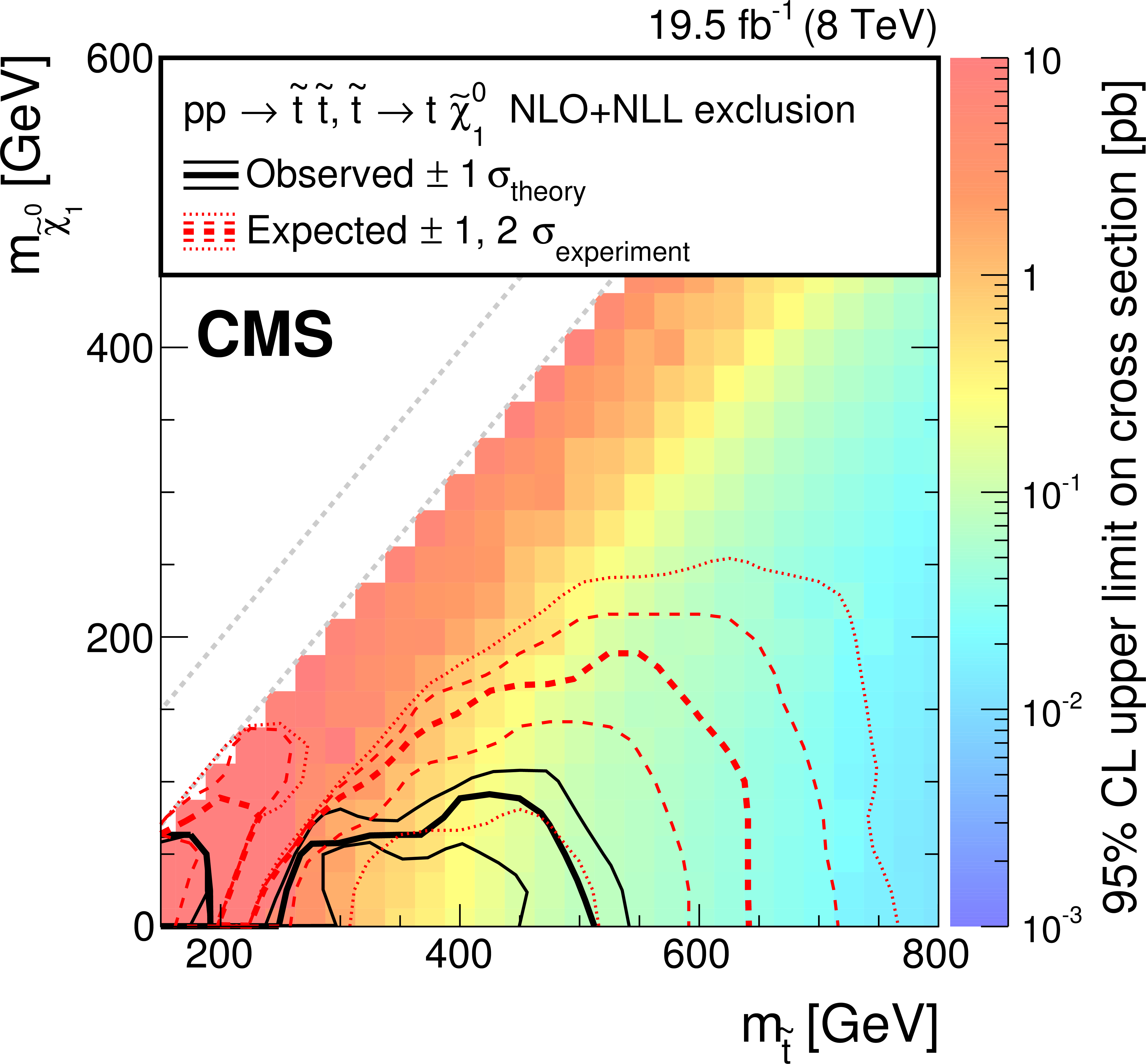
png pdf |
Figure 12-c:
5Exclusion limits at 95% CL for (upper left) direct squark production, (upper right) direct bottom-squark production, and (bottom) direct top-squark production. For the direct squark production, the upper set of curves corresponds to the scenario where the first two generations of squarks are degenerate and light, while the lower set corresponds to only one accessible light-flavour squark. For convenience, diagonal lines have been drawn corresponding to $ m_{ {\tilde{\chi}^{0}_{1}} } = m_{ \mathrm{ \tilde{q}, \tilde{b}, \tilde{t} } }$ and $ {m_{ {\tilde{\chi}^{0}_{1}} }} =m_{ \mathrm{ \tilde{q}, \tilde{b}, \tilde{t} } } - \left (m_{ {\mathrm {W}}} + {m_{ {\mathrm {b}} }} \right )$ where applicable. |
png pdf |
Figure 13-a:
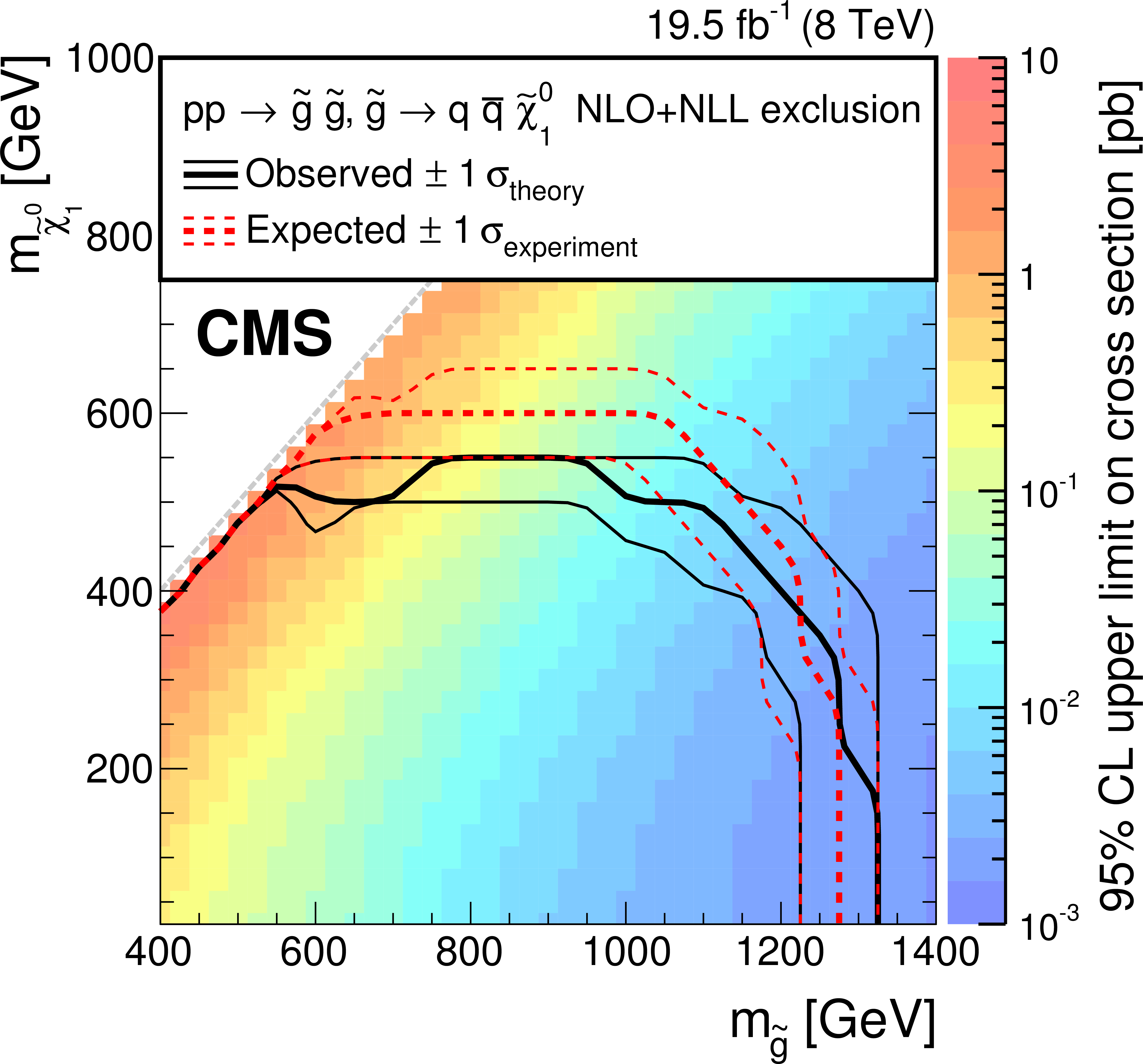
Exclusion limits at 95% CL for gluino mediated (upper left) squark production, (upper right) bottom-squark production, and (bottom) top-squark production. For convenience, diagonal lines have been drawn corresponding to $ m_{ {\tilde{\chi}^{0}_{1}} } = m_{\mathrm { \tilde{g} } } $ and $ m_{ {\tilde{\chi}^{0}_{1}} } = m_{\mathrm { \tilde{g} } } - m_{ {\mathrm {t}} } $ where applicable. |

png pdf |
Figure 13-b:
Exclusion limits at 95% CL for gluino mediated (upper left) squark production, (upper right) bottom-squark production, and (bottom) top-squark production. For convenience, diagonal lines have been drawn corresponding to $ m_{ {\tilde{\chi}^{0}_{1}} } = m_{\mathrm { \tilde{g} } } $ and $ m_{ {\tilde{\chi}^{0}_{1}} } = m_{\mathrm { \tilde{g} } } - m_{ {\mathrm {t}} } $ where applicable. |
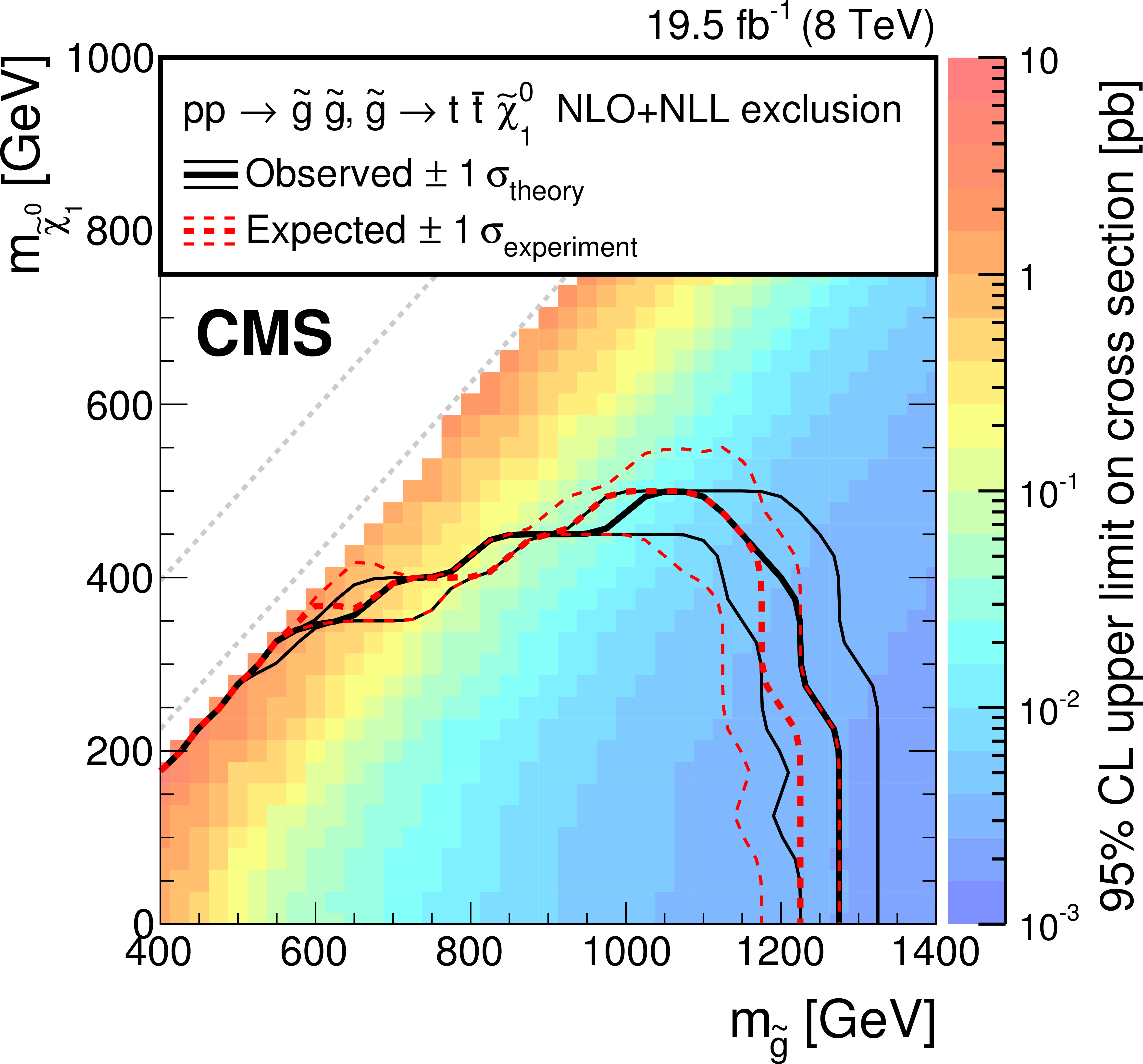
png pdf |
Figure 13-c:
Exclusion limits at 95% CL for gluino mediated (upper left) squark production, (upper right) bottom-squark production, and (bottom) top-squark production. For convenience, diagonal lines have been drawn corresponding to $ m_{ {\tilde{\chi}^{0}_{1}} } = m_{\mathrm { \tilde{g} } } $ and $ m_{ {\tilde{\chi}^{0}_{1}} } = m_{\mathrm { \tilde{g} } } - m_{ {\mathrm {t}} } $ where applicable. |
png pdf |
Figure 14:
Exclusion limits at 95% CL for gluino pair production with one gluino decaying via $ \mathrm { \tilde{g} } \to {\mathrm {q} \bar{q} } {\tilde{\chi}^{0}_{2}} $, $ {\tilde{\chi}^{0}_{2}} \to {\mathrm {h}} {\tilde{\chi}^{0}_{1}} $, while the other gluino decays via $ \mathrm { \tilde{g} } \to \mathrm { q q' } {\tilde{\chi}^{\pm }_{1}} $, $ {\tilde{\chi}^{\pm }_{1}} \to {\mathrm {W}}^\pm {\tilde{\chi}^{0}_{1}} $. For convenience, diagonal lines have been drawn corresponding to $ {m_{ {\tilde{\chi}^{0}_{1}} }} = m_{\mathrm { \tilde{g} } } $ and $ m_{ {\tilde{\chi}^{0}_{1}} } = m_{\mathrm { \tilde{g} }} - 200 $ GeV. |
png pdf |
Figure 15:
Exclusion limits at 95% CL as a function of $m_0$ and $m_{1/2}$ for the cMSSM/mSUGRA model with $\tan \beta =30$, $A_0 = -2 \max (m_0, m_{1/2})$, and $\mu >0$. Here, $m_{ \mathrm{ \tilde{q} } } $ is the average mass of the first-generation squarks. |
png pdf |
Figure 16:
Exclusion limits at 95% CL as a function of $ m_{ \mathrm{ \tilde{g} } } $ and $ m_{ \mathrm{ \tilde{q} } } $ for the cMSSM/mSUGRA model with $\tan\beta =30$, $A_0 = -2\max(m_0, m_{1/2})$, and $\mu >0$. Here, $m_{ \mathrm{ \tilde{q} } } $ is the average mass of the first-generation squarks. |
|
|
Compact Muon Solenoid LHC, CERN |
|

|

|

|

|

|