

Compact Muon Solenoid
LHC, CERN
| CMS-SUS-13-024 ; CERN-PH-EP-2014-073 | ||
| Search for top-squark pairs decaying into Higgs or Z bosons in pp collisions at $\sqrt{s}$ = 8 TeV | ||
| CMS Collaboration | ||
| 15 May 2014 | ||
| Phys. Lett. B 736 (2014) 371 | ||
| Abstract: A search for supersymmetry through the direct pair production of top squarks, with Higgs (H) or Z bosons in the decay chain, is performed using a data sample of proton-proton collisions at $\sqrt{s}$ = 8 TeV collected in 2012 with the CMS detector at the LHC. The sample corresponds to an integrated luminosity of 19.5 inverse-femtobarns. The search is performed using a selection of events containing leptons and bottom-quark jets. No evidence for a significant excess of events over the standard model background prediction is observed. The results are interpreted in the context of simplified supersymmetric models with pair production of a heavier top-squark mass eigenstate stop_2 decaying to a lighter top-squark mass eigenstate stop_1 via either stop_2 $\to$ H stop_1 or stop_2 $\to$ Z stop_1, followed in both cases by stop_1 $\to$ top neutralino, where the neutralino is an undetected, stable, lightest supersymmetric particle. The interpretation is performed in the region where the mass difference between the stop_2 and stop_1 states is approximately equal to the top-quark mass, m_(stop_2) - m_(stop_1) ~ m_(top), which is not probed by searches for direct stop_1 squark pair production. The analysis excludes top squarks with masses m(stop_2) less than 575 GeV and m(stop_1) less than 400 GeV at a 95% confidence level. | ||
| Links: e-print arXiv:1405.3886 [hep-ex] (PDF) ; CDS record ; inSPIRE record ; Public twiki page ; CADI line (restricted) ; | ||
| Figures | |
png pdf |
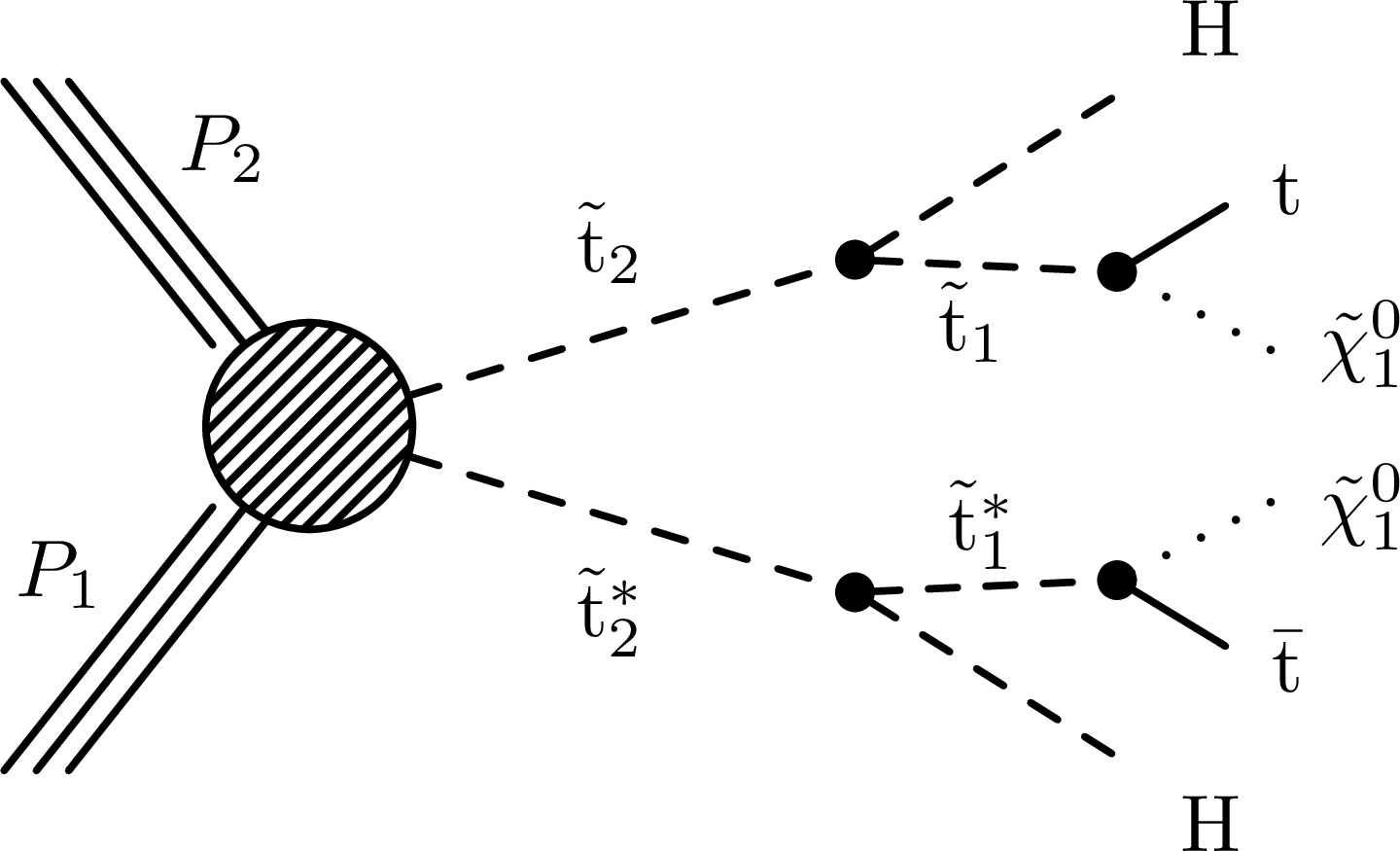
Figure 1-a:
Diagrams for the production of the heavier top-squark ($ {\tilde{t}_2} $) pairs followed by the decays $ {\tilde{t}_2} \to {\mathrm {H}} {\tilde{t}_1} $ or $ {\tilde{t}_2} \to {\mathrm {Z}} {\tilde{t}_1} $ with $ {\tilde{t}_1} \to {\mathrm {t}} \tilde{\chi}^{0}_{1} $. The symbol * denotes charge conjugation. |
png pdf |
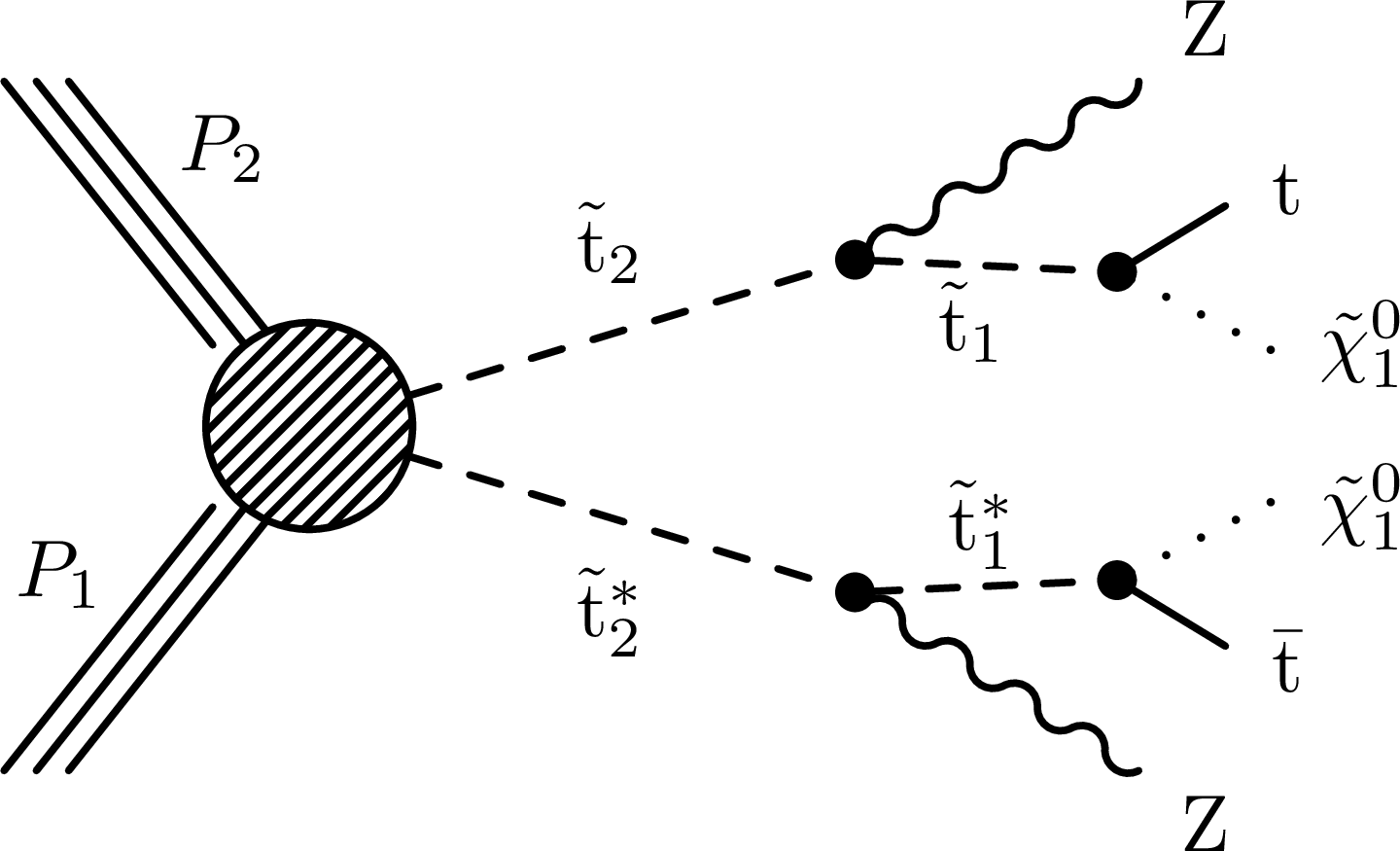
Figure 1-b:
Diagrams for the production of the heavier top-squark ($ {\tilde{t}_2} $) pairs followed by the decays $ {\tilde{t}_2} \to {\mathrm {H}} {\tilde{t}_1} $ or $ {\tilde{t}_2} \to {\mathrm {Z}} {\tilde{t}_1} $ with $ {\tilde{t}_1} \to {\mathrm {t}} \tilde{\chi}^{0}_{1} $. The symbol * denotes charge conjugation. |
png pdf |
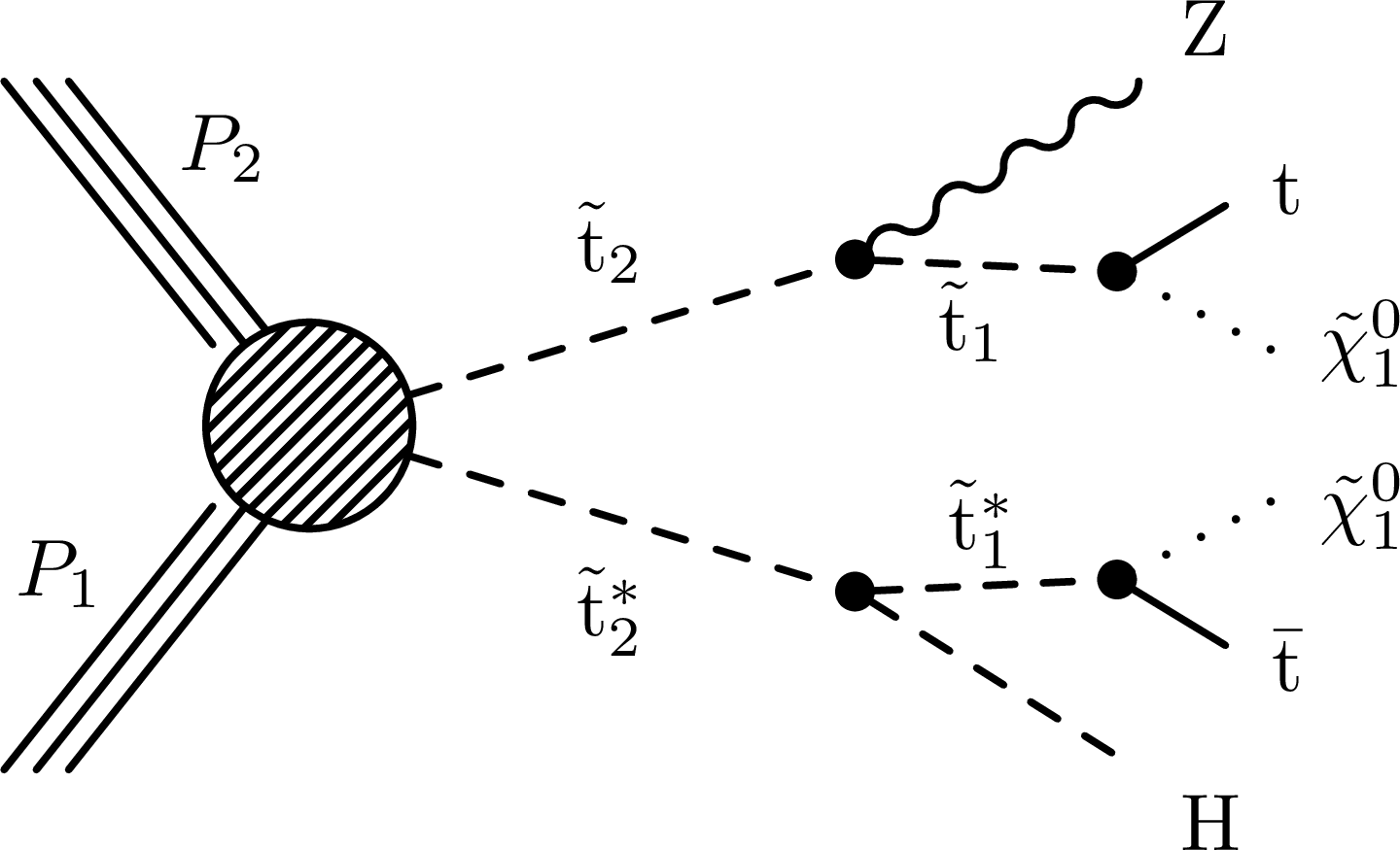
Figure 1-c:
Diagrams for the production of the heavier top-squark ($ {\tilde{t}_2} $) pairs followed by the decays $ {\tilde{t}_2} \to {\mathrm {H}} {\tilde{t}_1} $ or $ {\tilde{t}_2} \to {\mathrm {Z}} {\tilde{t}_1} $ with $ {\tilde{t}_1} \to {\mathrm {t}} \tilde{\chi}^{0}_{1} $. The symbol * denotes charge conjugation. |
png pdf |
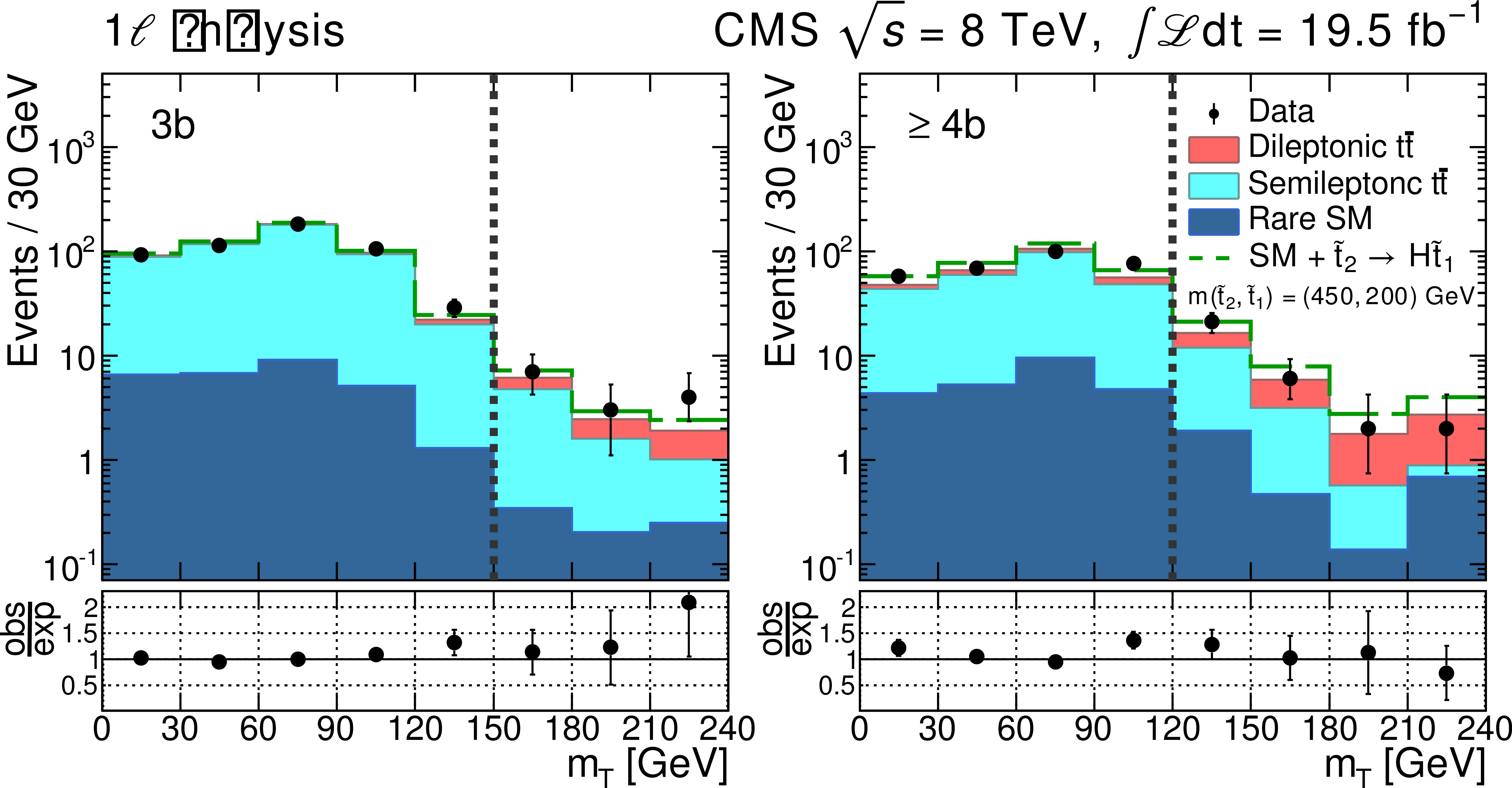
Figure 2-a:
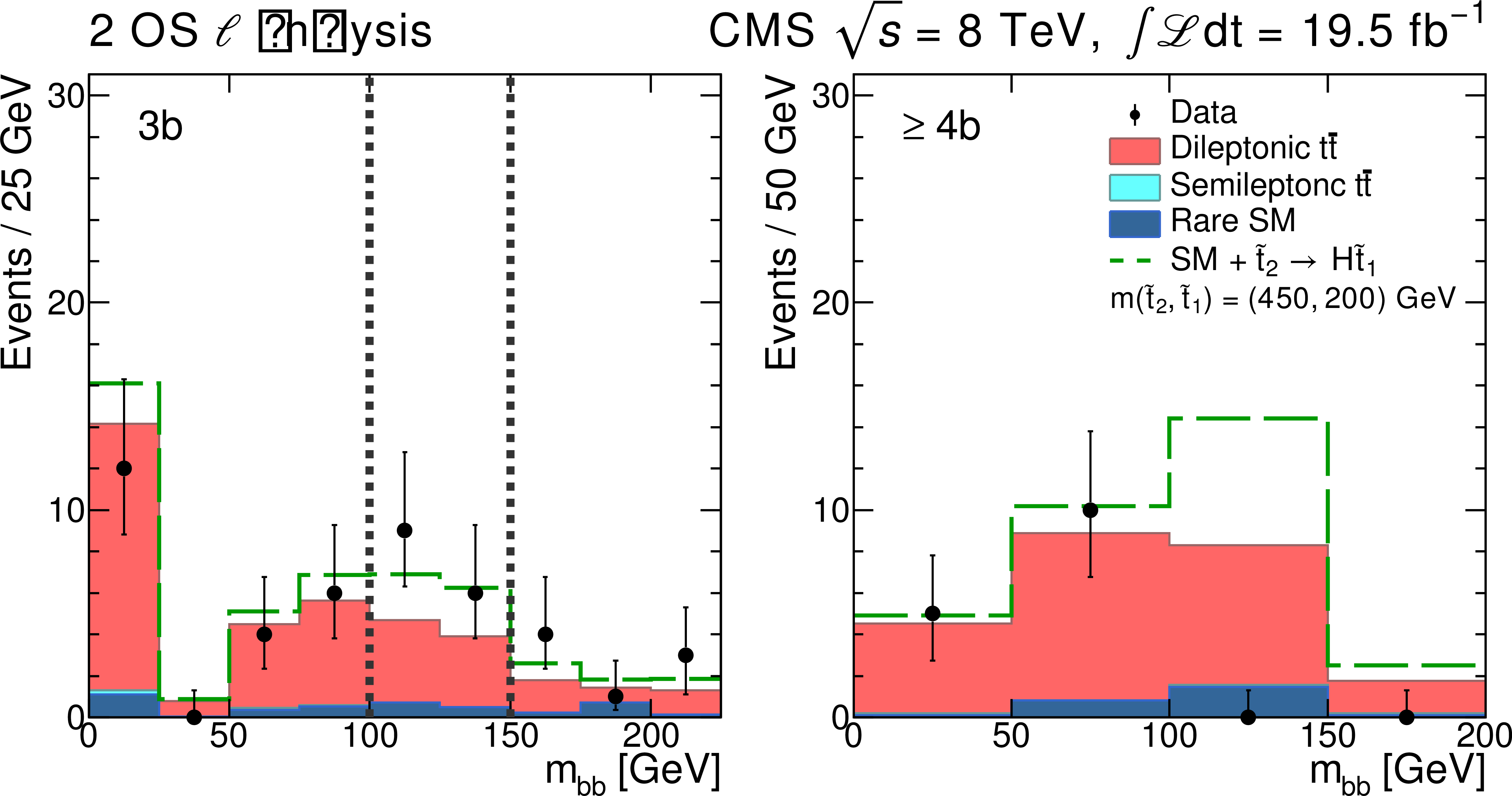
Comparison of the $ {m_{\mathrm {T}}} $ distributions for events with one lepton (a, b) and $ {m_{ {\mathrm {b}} {\mathrm {b}}}} $ distributions for events with two OS leptons (c, d) in data and MC simulation satisfying the $3 {\mathrm {b}}$ (a, c) and $\ge 4 {\mathrm {b}}$ (b, d) SR requirements. The vertical dashed lines indicate the corresponding signal region requirement. The semileptonic $ {\mathrm {t}\overline {\mathrm {t}}} $ and dileptonic $ {\mathrm {t}\overline {\mathrm {t}}} $ components represent simulated events characterized by the presence of one or two $ {\mathrm {W}}$ bosons decaying to $ {\mathrm {e}}$, $\mu $ or $\tau $. The yields of the $ {\mathrm {t}\overline {\mathrm {t}}} $ simulated samples are adjusted so that the total SM prediction is normalized to the data in the samples obtained by inverting the SR requirements. The distribution for the model $ {\tilde{t}_2} \to {\mathrm {H}} {\tilde{t}_1} $ where $m_{ {\tilde{t}_2} }=450$ GeV and $m_{ {\tilde{t}_1} }=200$ GeV is displayed on top of the backgrounds. The last bin contains the overflow events. The uncertainties in the background predictions are derived for the total yields in the signal regions and are listed in Table . |
png pdf |
Figure 2-b:
Comparison of the $ {m_{\mathrm {T}}} $ distributions for events with one lepton (a, b) and $ {m_{ {\mathrm {b}} {\mathrm {b}}}} $ distributions for events with two OS leptons (c, d) in data and MC simulation satisfying the $3 {\mathrm {b}}$ (a, c) and $\ge 4 {\mathrm {b}}$ (b, d) SR requirements. The vertical dashed lines indicate the corresponding signal region requirement. The semileptonic $ {\mathrm {t}\overline {\mathrm {t}}} $ and dileptonic $ {\mathrm {t}\overline {\mathrm {t}}} $ components represent simulated events characterized by the presence of one or two $ {\mathrm {W}}$ bosons decaying to $ {\mathrm {e}}$, $\mu $ or $\tau $. The yields of the $ {\mathrm {t}\overline {\mathrm {t}}} $ simulated samples are adjusted so that the total SM prediction is normalized to the data in the samples obtained by inverting the SR requirements. The distribution for the model $ {\tilde{t}_2} \to {\mathrm {H}} {\tilde{t}_1} $ where $m_{ {\tilde{t}_2} }=450$ GeV and $m_{ {\tilde{t}_1} }=200$ GeV is displayed on top of the backgrounds. The last bin contains the overflow events. The uncertainties in the background predictions are derived for the total yields in the signal regions and are listed in Table . |
png pdf |
Figure 3-a:
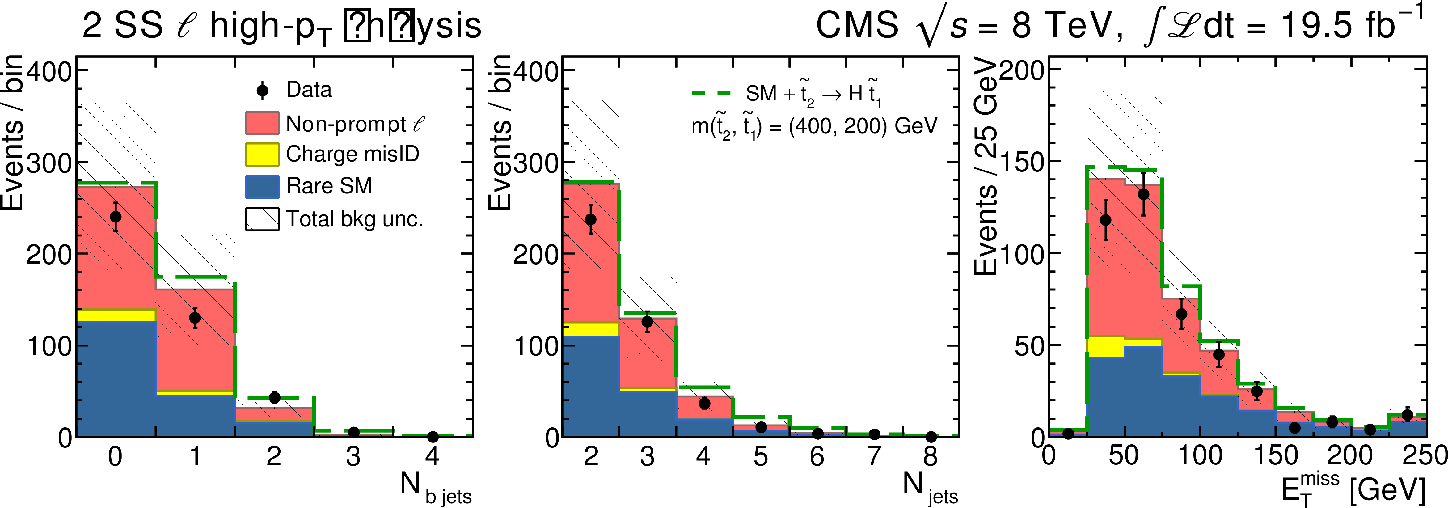
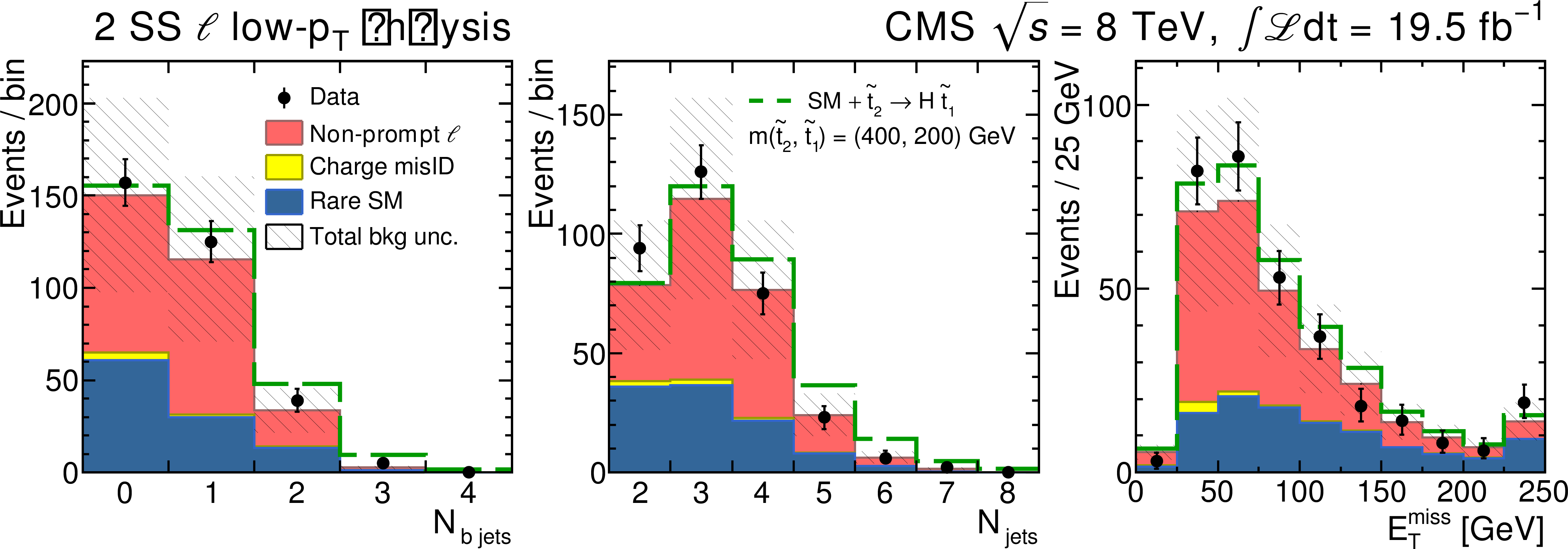
Data and predicted SM background for the event sample with two SS leptons as a function of number of $ { {\mathrm {b}}{\text { jets}}} $, number of jets, and $ {E_{\mathrm {T}}^{\text {miss}}} $ for events satisfying the high-$ {p_{\mathrm {T}}} $ (a, b, c) or the low-$ {p_{\mathrm {T}}} $ (d, e, f) selection. The shaded bands correspond to the total estimated uncertainty in the background prediction. The distribution for the model $ {\tilde{t}_2} \to {\mathrm {H}} {\tilde{t}_1} $ where $m_{ {\tilde{t}_2} }=$ 400 GeV and $m_{ {\tilde{t}_1} }=$200 GeV is displayed on top of the backgrounds. The last bin in the histograms includes overflow events. |
png pdf |
Figure 3-b:
Data and predicted SM background for the event sample with two SS leptons as a function of number of $ { {\mathrm {b}}{\text { jets}}} $, number of jets, and $ {E_{\mathrm {T}}^{\text {miss}}} $ for events satisfying the high-$ {p_{\mathrm {T}}} $ (a, b, c) or the low-$ {p_{\mathrm {T}}} $ (d, e, f) selection. The shaded bands correspond to the total estimated uncertainty in the background prediction. The distribution for the model $ {\tilde{t}_2} \to {\mathrm {H}} {\tilde{t}_1} $ where $m_{ {\tilde{t}_2} }=$ 400 GeV and $m_{ {\tilde{t}_1} }=$200 GeV is displayed on top of the backgrounds. The last bin in the histograms includes overflow events. |
png pdf |
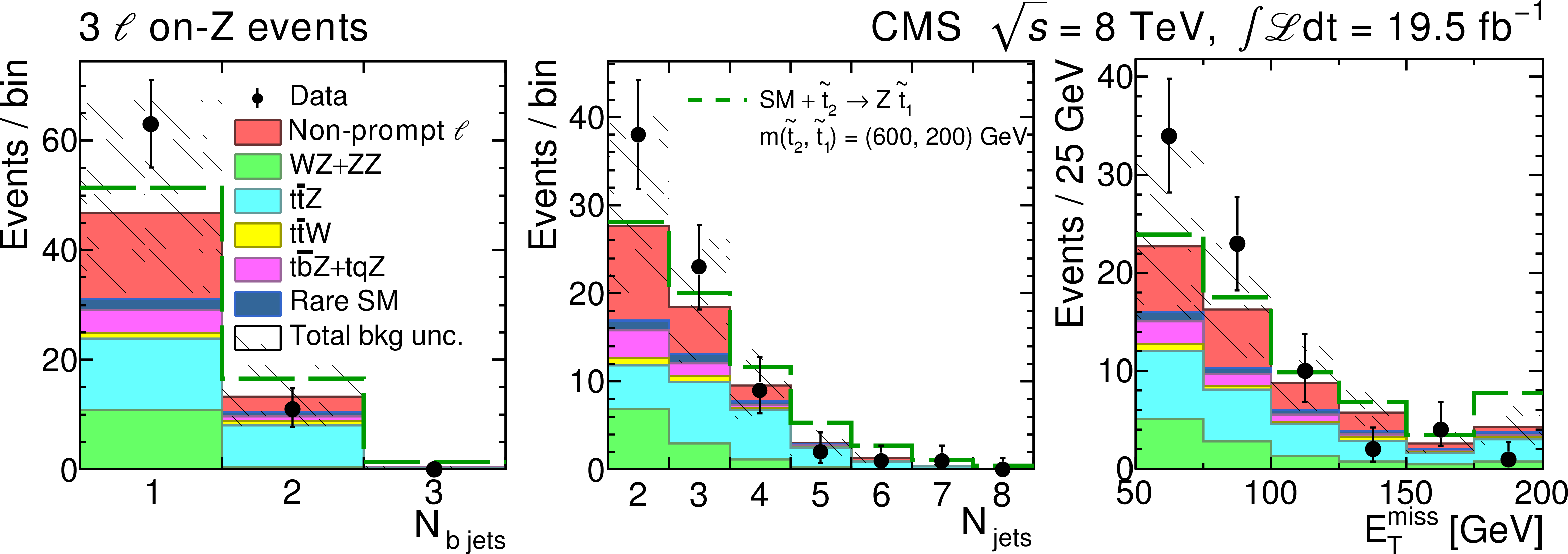
Figure 4-a:
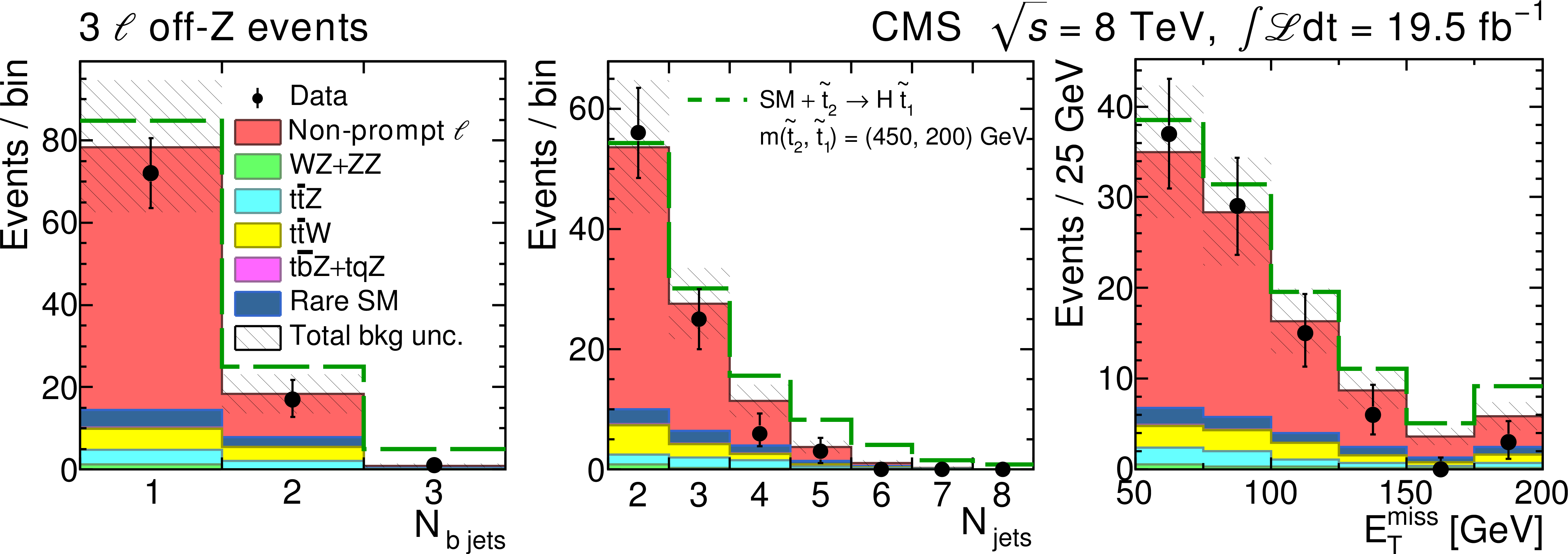
Data and predicted SM background for the event sample with at least three leptons as a function of number of $ { {\mathrm {b}}{\text { jets}}} $, number of jets, and $ {E_{\mathrm {T}}^{\text {miss}}} $ for events that do not contain (off-$ {\mathrm {Z}}$), (a, b, c), or contain (on-$ {\mathrm {Z}}$), (d, e, f), an OS same-flavor pair that is a $ {\mathrm {Z}}$ boson candidate. The shaded bands correspond to the total estimated uncertainty in the background prediction. The distributions for the models $ {\tilde{t}_2} \to {\mathrm {H}} {\tilde{t}_1} $ and $ {\tilde{t}_2} \to {\mathrm {Z}} {\tilde{t}_1} $ are displayed on top of the backgrounds in the top and bottom rows respectively. The top-squark masses are $m_{ {\tilde{t}_1} }=$ 200 GeV and $m_{ {\tilde{t}_2} }=$ (450, 600) GeV for the $( {\mathrm {H}} , {\mathrm {Z}})$ channel. The last bin in the histograms includes overflow events. |
png pdf |
Figure 4-b:
Data and predicted SM background for the event sample with at least three leptons as a function of number of $ { {\mathrm {b}}{\text { jets}}} $, number of jets, and $ {E_{\mathrm {T}}^{\text {miss}}} $ for events that do not contain (off-$ {\mathrm {Z}}$), (a, b, c), or contain (on-$ {\mathrm {Z}}$), (d, e, f), an OS same-flavor pair that is a $ {\mathrm {Z}}$ boson candidate. The shaded bands correspond to the total estimated uncertainty in the background prediction. The distributions for the models $ {\tilde{t}_2} \to {\mathrm {H}} {\tilde{t}_1} $ and $ {\tilde{t}_2} \to {\mathrm {Z}} {\tilde{t}_1} $ are displayed on top of the backgrounds in the top and bottom rows respectively. The top-squark masses are $m_{ {\tilde{t}_1} }=$ 200 GeV and $m_{ {\tilde{t}_2} }=$ (450, 600) GeV for the $( {\mathrm {H}} , {\mathrm {Z}})$ channel. The last bin in the histograms includes overflow events. |
png pdf |
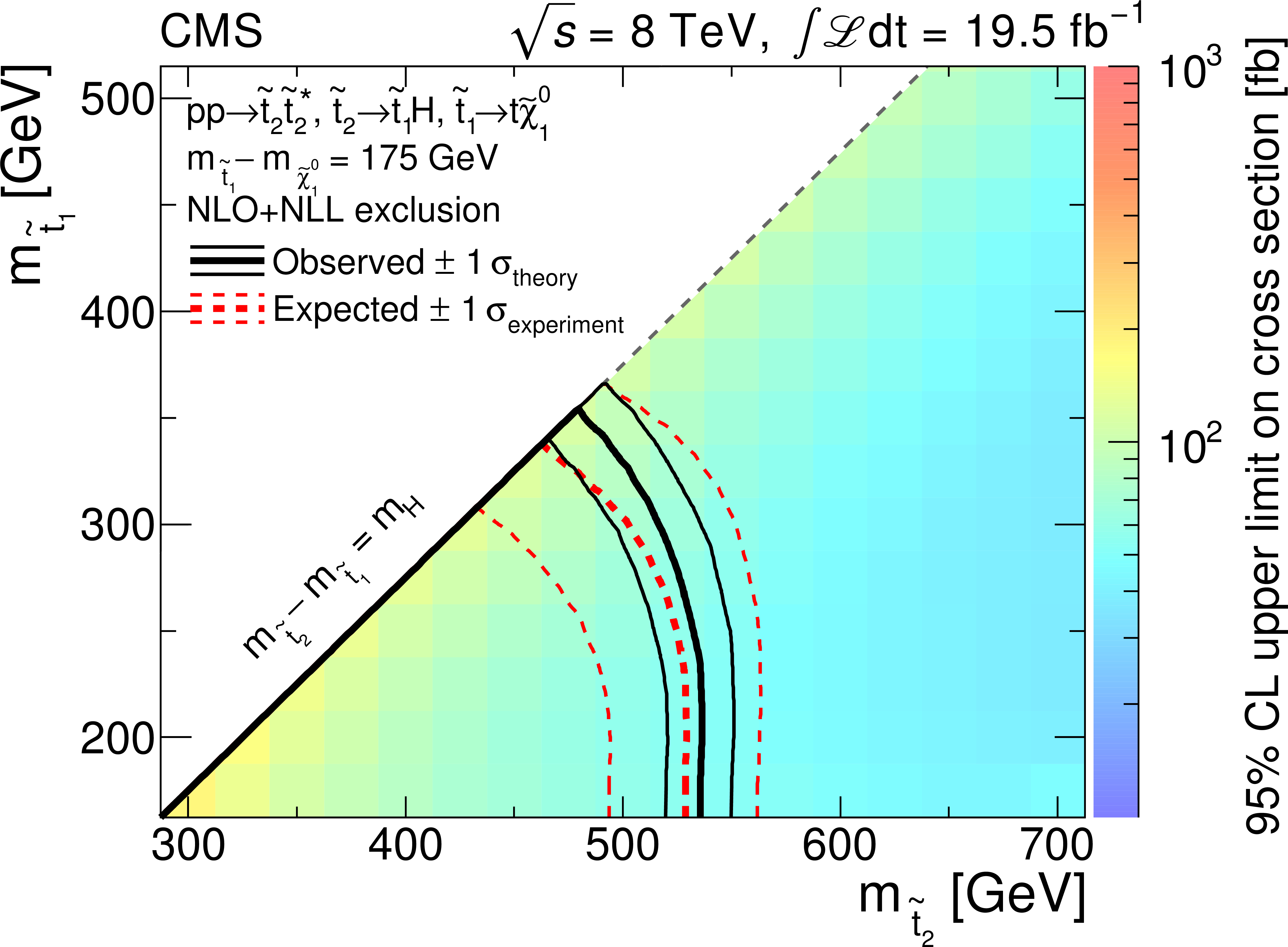
Figure 5-a:
Interpretation of the results in SUSY simplified model parameter space, $m_{ {\tilde{t}_1} }$ vs. $m_{ {\tilde{t}_2} }$, with the neutralino mass constrained by the relation $m_{ {\tilde{t}_1} } - m_{ {\tilde{\chi}^{0}_{1}} } = $ 175 GeV. The shaded maps (a, c) show the upper limit (95% CL) on the cross section times branching fraction at each point in the $m_{ {\tilde{t}_1} }$ vs. $m_{ {\tilde{t}_2} }$ plane for the process $ {\mathrm {p}} {\mathrm {p}}\to {\tilde{t}_2} {\tilde{t}_2} ^{*}$, with $ {\tilde{t}_2} \to {\mathrm {H}} {\tilde{t}_1} $, $ {\tilde{t}_1} \to {\mathrm {t}} {\tilde{\chi}^{0}_{1}} $ (a, b) and $ {\tilde{t}_2} \to {\mathrm {Z}} {\tilde{t}_1} $, $ {\tilde{t}_1} \to {\mathrm {t}} {\tilde{\chi}^{0}_{1}} $ (c, d). In these plots, the results from all channels are combined. The excluded region in the $m_{ {\tilde{t}_1} }$vs. $m_{ {\tilde{t}_2} }$ parameter space is obtained by comparing the cross section times branching fraction upper limit at each model point with the corresponding NLO+NLL cross section for the process, assuming that (a) $\mathcal {B}( {\tilde{t}_2} \to {\mathrm {H}} {\tilde{t}_1} )=$100% or (b) that $\mathcal {B}( {\tilde{t}_2} \to {\mathrm {Z}} {\tilde{t}_1} )=$ 100%. The solid (dashed) curves define the boundary of the observed (expected) excluded region. The $\pm $1 standard deviation ($\sigma $) bands are indicated by the finer contours. The figures on the right show the observed (expected) exclusion contours, which are indicated by the solid (dashed) curves for the contributing channels. As indicated in the legends of the right-hand figures, the thinner curves show the results from each of the contributing channels, while the thicker curve shows their combination. The four event categories for the $ {\tilde{t}_2} \to {\mathrm {H}} {\tilde{t}_1} $ study are shown in the upper plots, while the on-$ {\mathrm {Z}}$ and off-$ {\mathrm {Z}}$ categories for events with at least three leptons are shown in the lower plots. |

png pdf |
Figure 5-b:
Interpretation of the results in SUSY simplified model parameter space, $m_{ {\tilde{t}_1} }$ vs. $m_{ {\tilde{t}_2} }$, with the neutralino mass constrained by the relation $m_{ {\tilde{t}_1} } - m_{ {\tilde{\chi}^{0}_{1}} } = $ 175 GeV. The shaded maps (a, c) show the upper limit (95% CL) on the cross section times branching fraction at each point in the $m_{ {\tilde{t}_1} }$ vs. $m_{ {\tilde{t}_2} }$ plane for the process $ {\mathrm {p}} {\mathrm {p}}\to {\tilde{t}_2} {\tilde{t}_2} ^{*}$, with $ {\tilde{t}_2} \to {\mathrm {H}} {\tilde{t}_1} $, $ {\tilde{t}_1} \to {\mathrm {t}} {\tilde{\chi}^{0}_{1}} $ (a, b) and $ {\tilde{t}_2} \to {\mathrm {Z}} {\tilde{t}_1} $, $ {\tilde{t}_1} \to {\mathrm {t}} {\tilde{\chi}^{0}_{1}} $ (c, d). In these plots, the results from all channels are combined. The excluded region in the $m_{ {\tilde{t}_1} }$vs. $m_{ {\tilde{t}_2} }$ parameter space is obtained by comparing the cross section times branching fraction upper limit at each model point with the corresponding NLO+NLL cross section for the process, assuming that (a) $\mathcal {B}( {\tilde{t}_2} \to {\mathrm {H}} {\tilde{t}_1} )=$100% or (b) that $\mathcal {B}( {\tilde{t}_2} \to {\mathrm {Z}} {\tilde{t}_1} )=$ 100%. The solid (dashed) curves define the boundary of the observed (expected) excluded region. The $\pm $1 standard deviation ($\sigma $) bands are indicated by the finer contours. The figures on the right show the observed (expected) exclusion contours, which are indicated by the solid (dashed) curves for the contributing channels. As indicated in the legends of the right-hand figures, the thinner curves show the results from each of the contributing channels, while the thicker curve shows their combination. The four event categories for the $ {\tilde{t}_2} \to {\mathrm {H}} {\tilde{t}_1} $ study are shown in the upper plots, while the on-$ {\mathrm {Z}}$ and off-$ {\mathrm {Z}}$ categories for events with at least three leptons are shown in the lower plots. |
png pdf |
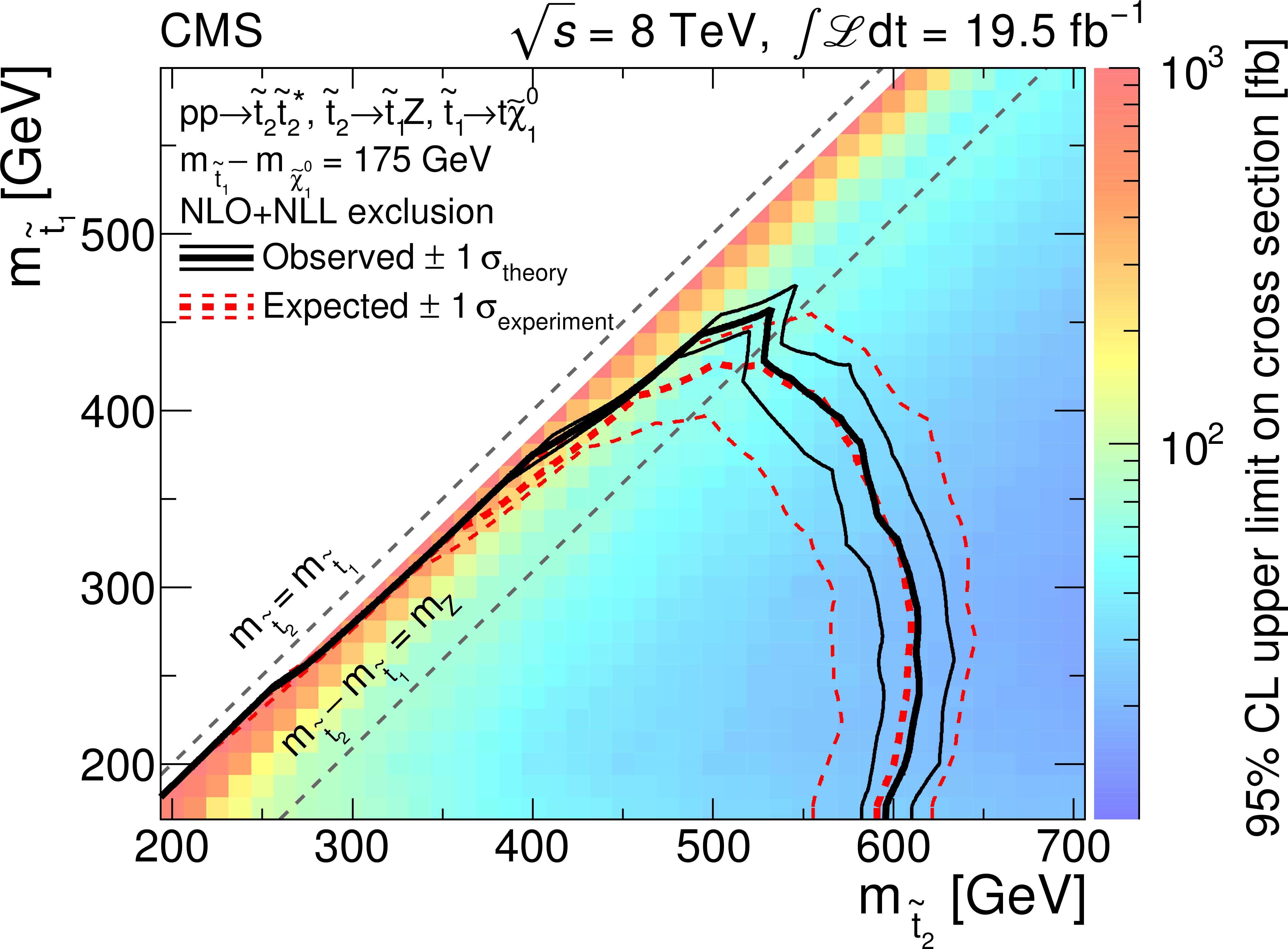
Figure 5-c:
Interpretation of the results in SUSY simplified model parameter space, $m_{ {\tilde{t}_1} }$ vs. $m_{ {\tilde{t}_2} }$, with the neutralino mass constrained by the relation $m_{ {\tilde{t}_1} } - m_{ {\tilde{\chi}^{0}_{1}} } = $ 175 GeV. The shaded maps (a, c) show the upper limit (95% CL) on the cross section times branching fraction at each point in the $m_{ {\tilde{t}_1} }$ vs. $m_{ {\tilde{t}_2} }$ plane for the process $ {\mathrm {p}} {\mathrm {p}}\to {\tilde{t}_2} {\tilde{t}_2} ^{*}$, with $ {\tilde{t}_2} \to {\mathrm {H}} {\tilde{t}_1} $, $ {\tilde{t}_1} \to {\mathrm {t}} {\tilde{\chi}^{0}_{1}} $ (a, b) and $ {\tilde{t}_2} \to {\mathrm {Z}} {\tilde{t}_1} $, $ {\tilde{t}_1} \to {\mathrm {t}} {\tilde{\chi}^{0}_{1}} $ (c, d). In these plots, the results from all channels are combined. The excluded region in the $m_{ {\tilde{t}_1} }$vs. $m_{ {\tilde{t}_2} }$ parameter space is obtained by comparing the cross section times branching fraction upper limit at each model point with the corresponding NLO+NLL cross section for the process, assuming that (a) $\mathcal {B}( {\tilde{t}_2} \to {\mathrm {H}} {\tilde{t}_1} )=$100% or (b) that $\mathcal {B}( {\tilde{t}_2} \to {\mathrm {Z}} {\tilde{t}_1} )=$ 100%. The solid (dashed) curves define the boundary of the observed (expected) excluded region. The $\pm $1 standard deviation ($\sigma $) bands are indicated by the finer contours. The figures on the right show the observed (expected) exclusion contours, which are indicated by the solid (dashed) curves for the contributing channels. As indicated in the legends of the right-hand figures, the thinner curves show the results from each of the contributing channels, while the thicker curve shows their combination. The four event categories for the $ {\tilde{t}_2} \to {\mathrm {H}} {\tilde{t}_1} $ study are shown in the upper plots, while the on-$ {\mathrm {Z}}$ and off-$ {\mathrm {Z}}$ categories for events with at least three leptons are shown in the lower plots. |
png pdf |
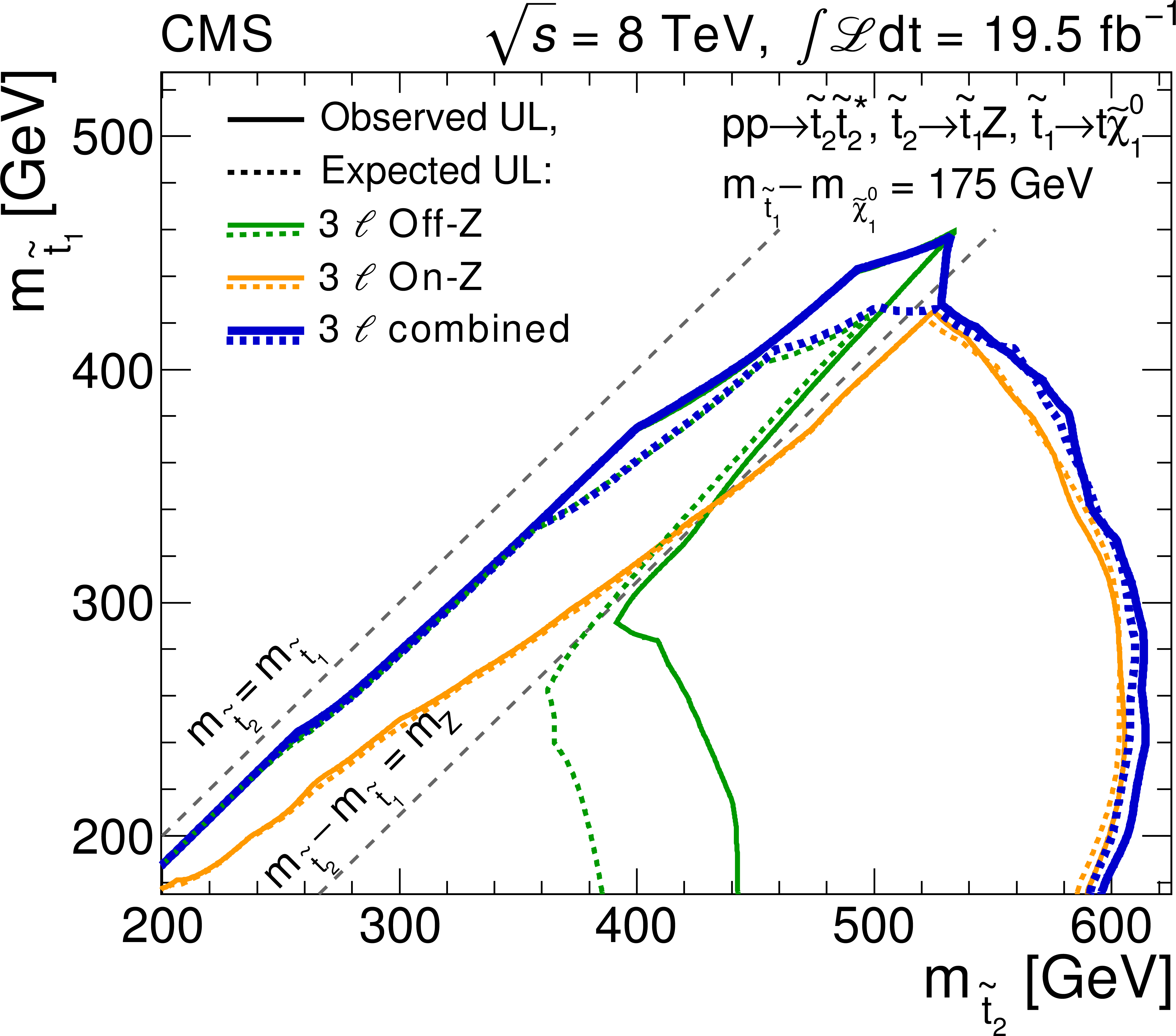
Figure 5-d:
Interpretation of the results in SUSY simplified model parameter space, $m_{ {\tilde{t}_1} }$ vs. $m_{ {\tilde{t}_2} }$, with the neutralino mass constrained by the relation $m_{ {\tilde{t}_1} } - m_{ {\tilde{\chi}^{0}_{1}} } = $ 175 GeV. The shaded maps (a, c) show the upper limit (95% CL) on the cross section times branching fraction at each point in the $m_{ {\tilde{t}_1} }$ vs. $m_{ {\tilde{t}_2} }$ plane for the process $ {\mathrm {p}} {\mathrm {p}}\to {\tilde{t}_2} {\tilde{t}_2} ^{*}$, with $ {\tilde{t}_2} \to {\mathrm {H}} {\tilde{t}_1} $, $ {\tilde{t}_1} \to {\mathrm {t}} {\tilde{\chi}^{0}_{1}} $ (a, b) and $ {\tilde{t}_2} \to {\mathrm {Z}} {\tilde{t}_1} $, $ {\tilde{t}_1} \to {\mathrm {t}} {\tilde{\chi}^{0}_{1}} $ (c, d). In these plots, the results from all channels are combined. The excluded region in the $m_{ {\tilde{t}_1} }$vs. $m_{ {\tilde{t}_2} }$ parameter space is obtained by comparing the cross section times branching fraction upper limit at each model point with the corresponding NLO+NLL cross section for the process, assuming that (a) $\mathcal {B}( {\tilde{t}_2} \to {\mathrm {H}} {\tilde{t}_1} )=$100% or (b) that $\mathcal {B}( {\tilde{t}_2} \to {\mathrm {Z}} {\tilde{t}_1} )=$ 100%. The solid (dashed) curves define the boundary of the observed (expected) excluded region. The $\pm $1 standard deviation ($\sigma $) bands are indicated by the finer contours. The figures on the right show the observed (expected) exclusion contours, which are indicated by the solid (dashed) curves for the contributing channels. As indicated in the legends of the right-hand figures, the thinner curves show the results from each of the contributing channels, while the thicker curve shows their combination. The four event categories for the $ {\tilde{t}_2} \to {\mathrm {H}} {\tilde{t}_1} $ study are shown in the upper plots, while the on-$ {\mathrm {Z}}$ and off-$ {\mathrm {Z}}$ categories for events with at least three leptons are shown in the lower plots. |

png pdf |
Figure 6:
Upper limits on the cross section for $ {\tilde{t}_2} $ pair production for different branching fractions of $ {\tilde{t}_2} \to {\mathrm {H}} {\tilde{t}_1} $ and $ {\tilde{t}_2} \to {\mathrm {Z}} {\tilde{t}_1} $, assuming that $\mathcal {B}( {\tilde{t}_2} \to {\mathrm {H}} {\tilde{t}_1} ) + \mathcal {B}( {\tilde{t}_2} \to {\mathrm {Z}} {\tilde{t}_1} ) =$ 100%. The $ {\tilde{t}_1} $ squark is assumed to always decay to a top quark and a neutralino $ {\tilde{\chi}^{0}_{1}} $ with $m_{ {\tilde{t}_1} } - m_{ {\tilde{\chi}^{0}_{1}} } = m_{ {\mathrm {t}}}$. The decay $ {\tilde{t}_2} \to {\mathrm {H}} {\tilde{t}_1} $ is only considered when the $ {\mathrm {H}} $ boson production is kinematically allowed, $m_{ {\tilde{t}_2} }-m_{ {\tilde{t}_1} }>m_{ {\mathrm {H}} }$. |
|
|
Compact Muon Solenoid LHC, CERN |
|

|

|

|

|

|