

Compact Muon Solenoid
LHC, CERN
| CMS-TAU-14-001 ; CERN-PH-EP-2015-261 | ||
| Reconstruction and identification of $\tau$ lepton decays to hadrons and $\nu_\tau$ at CMS | ||
| CMS Collaboration | ||
| 26 October 2015 | ||
| Accepted for publication in J. Instrum. J. Instrum. 11 (2016) P01019 | ||
| Abstract: This paper describes the algorithms used by the CMS experiment to reconstruct and identify $\tau \to \text{hadrons} + \nu_\tau$ decays during Run 1 of the LHC. The performance of the algorithms is studied in proton-proton collisions recorded at a centre-of-mass energy of 8 TeV, corresponding to an integrated luminosity of 19.7 fb$^{-1}$. The algorithms achieve an identification efficiency of 50-60%, with misidentification rates for quark and gluon jets, electrons, and muons between per mille and per cent levels. | ||
| Links: e-print arXiv:1510.07488 [physics.ins-det] (PDF) ; CDS record ; inSPIRE record ; CADI line (restricted) ; | ||
| Figures | |
png pdf |
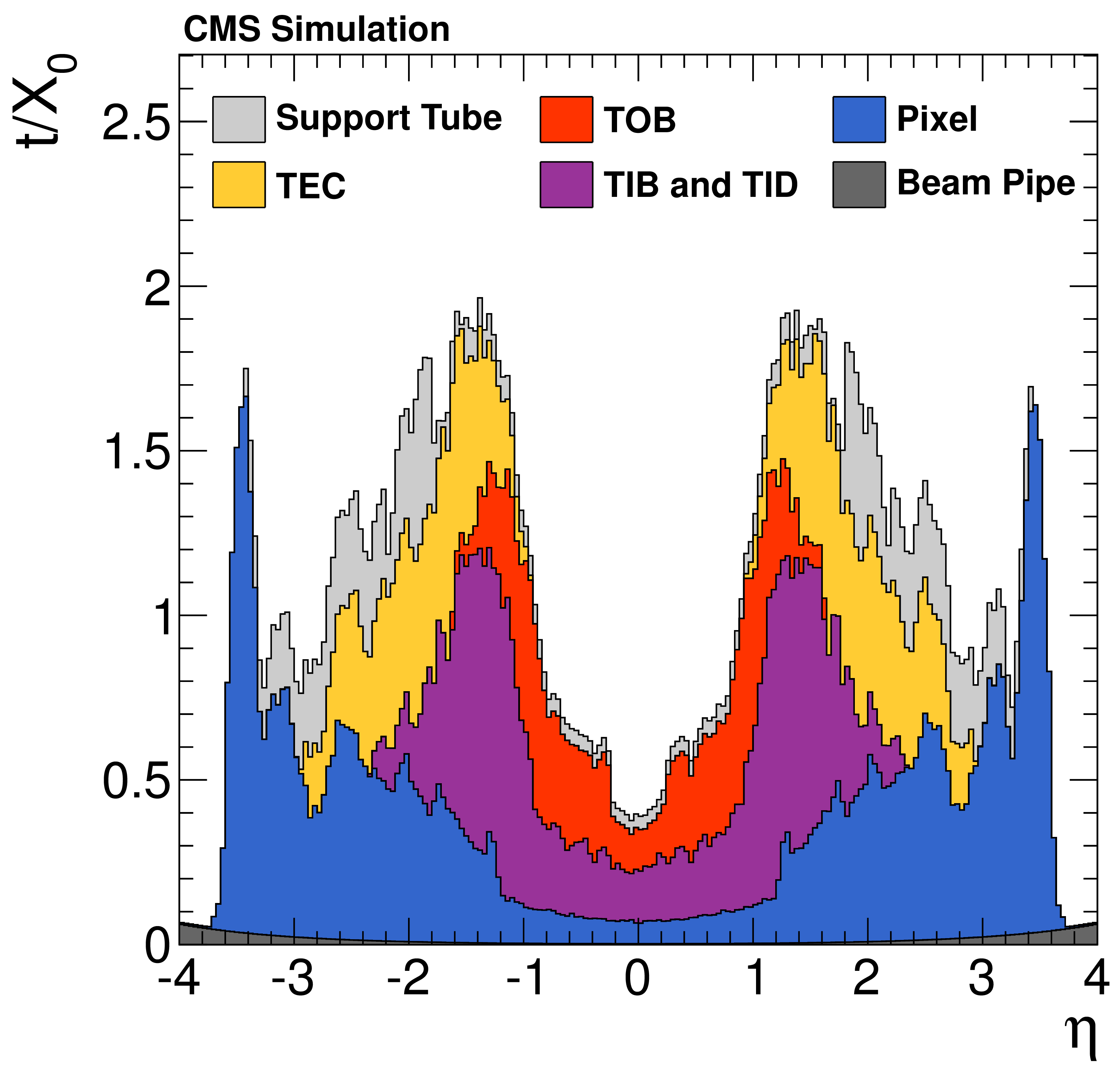
Figure 1:
The total material thickness ($t$) in units of radiation length $X_{0}$, as a function of $\eta $, that a particle produced at the interaction point must traverse before it reaches the ECAL. The material used for sensors, readout electronics, mechanical structures, cooling, and services is given separately for the silicon pixel detector and for individual components of the silicon strip detector (``TEC'', ``TOB'', ``TIB and TID'') [21]. The material used for the beam pipe and for the support tube that separates the tracker from the ECAL is also shown separately. |

png pdf |
Figure 2-a:
Transverse momentum distributions of the visible decay products of $ { {\tau }_{\mathrm {h}}} $ decays, in (a) simulated $ {\mathrm {Z}}/ { {\gamma } ^{*}} \to {\tau } {\tau }$ events, (b) $ { {\mathrm {Z}}'} (2.5 TeV ) \to {\tau } {\tau }$ events, and (c) of quark and gluon jets in simulated W+jets and multijet events, at the generator level. |
png pdf |
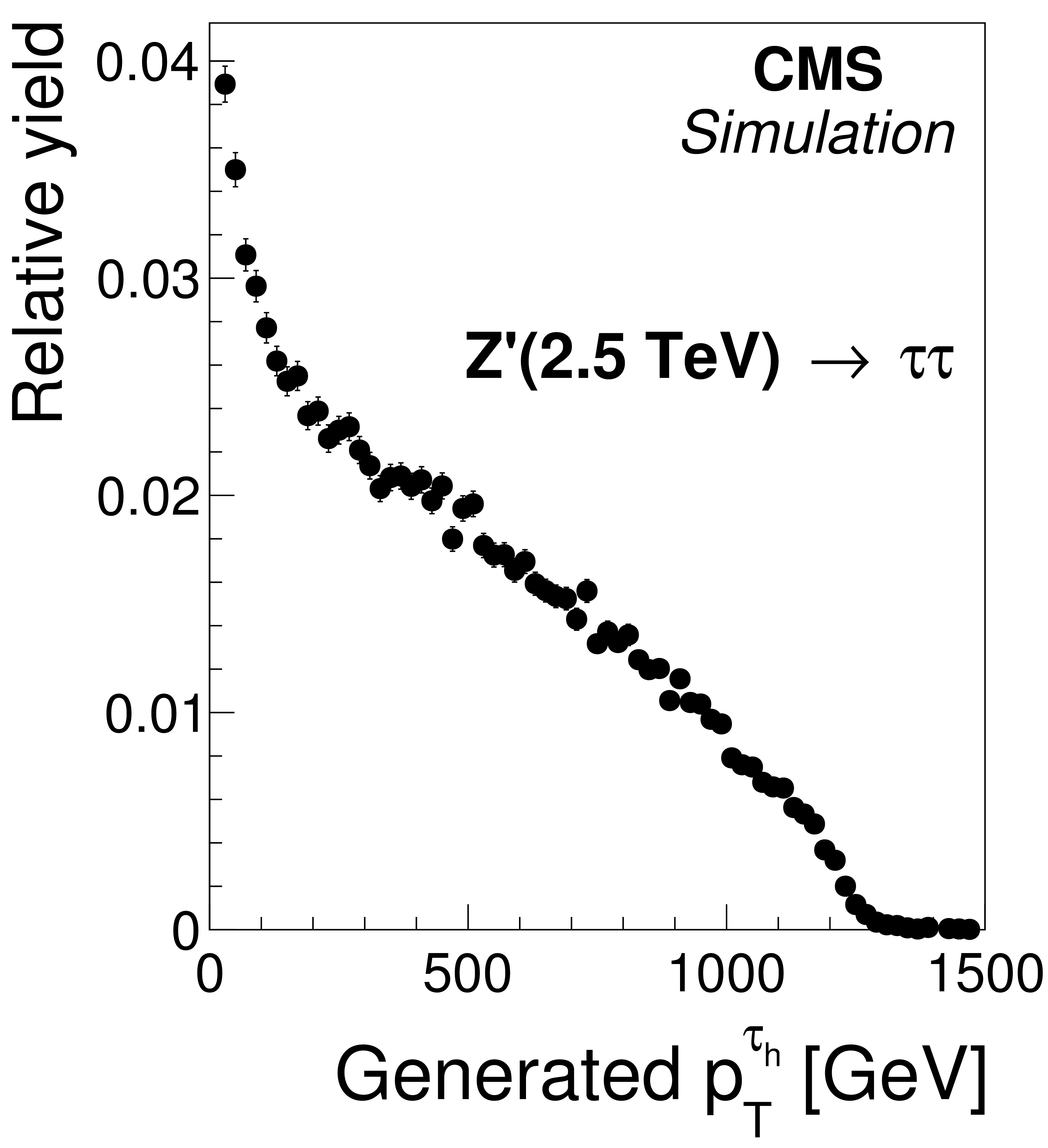
Figure 2-b:
Transverse momentum distributions of the visible decay products of $ { {\tau }_{\mathrm {h}}} $ decays, in (a) simulated $ {\mathrm {Z}}/ { {\gamma } ^{*}} \to {\tau } {\tau }$ events, (b) $ { {\mathrm {Z}}'} (2.5 TeV ) \to {\tau } {\tau }$ events, and (c) of quark and gluon jets in simulated W+jets and multijet events, at the generator level. |
png pdf |
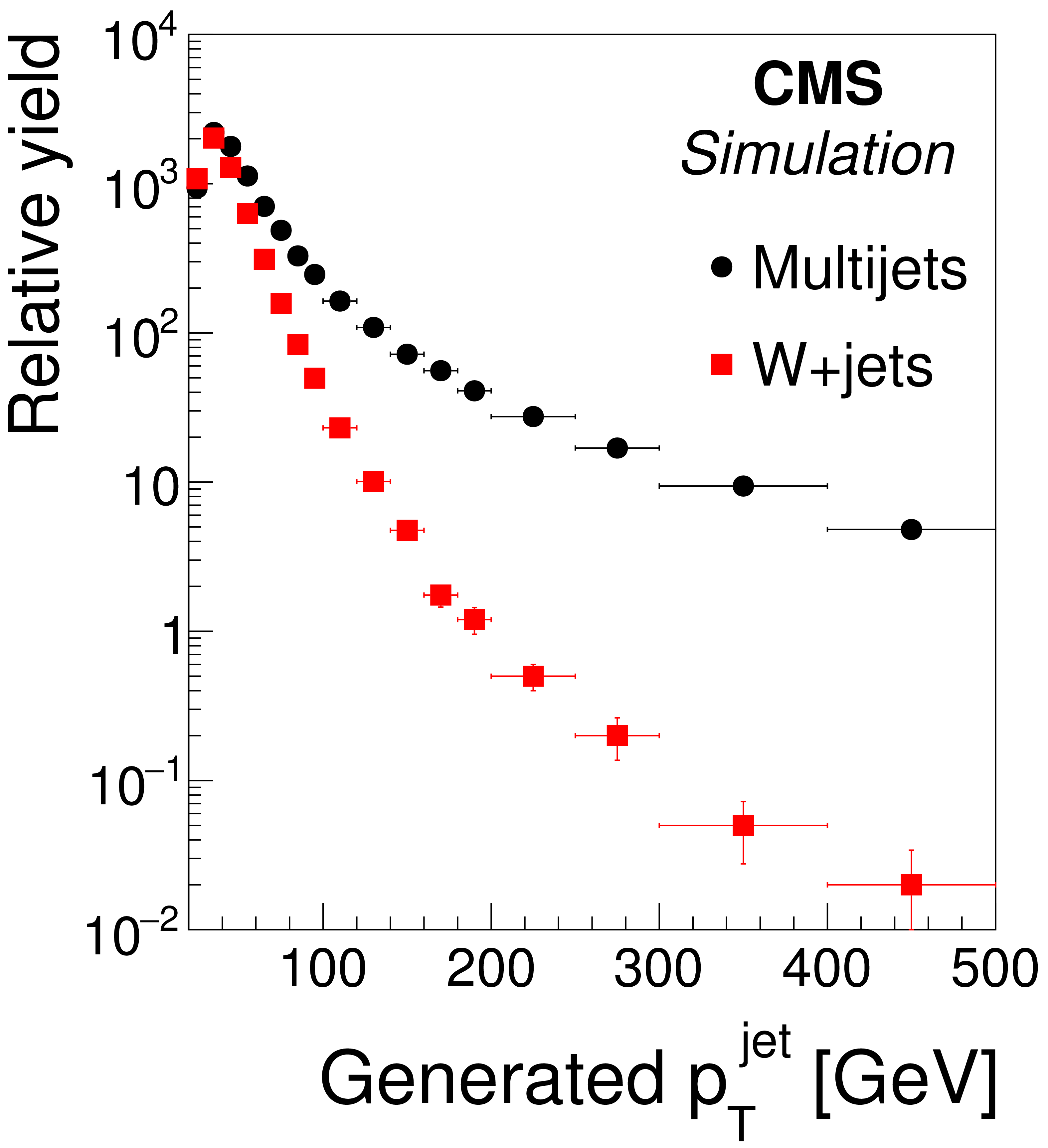
Figure 2-c:
Transverse momentum distributions of the visible decay products of $ { {\tau }_{\mathrm {h}}} $ decays, in (a) simulated $ {\mathrm {Z}}/ { {\gamma } ^{*}} \to {\tau } {\tau }$ events, (b) $ { {\mathrm {Z}}'} (2.5 TeV ) \to {\tau } {\tau }$ events, and (c) of quark and gluon jets in simulated W+jets and multijet events, at the generator level. |
png pdf |
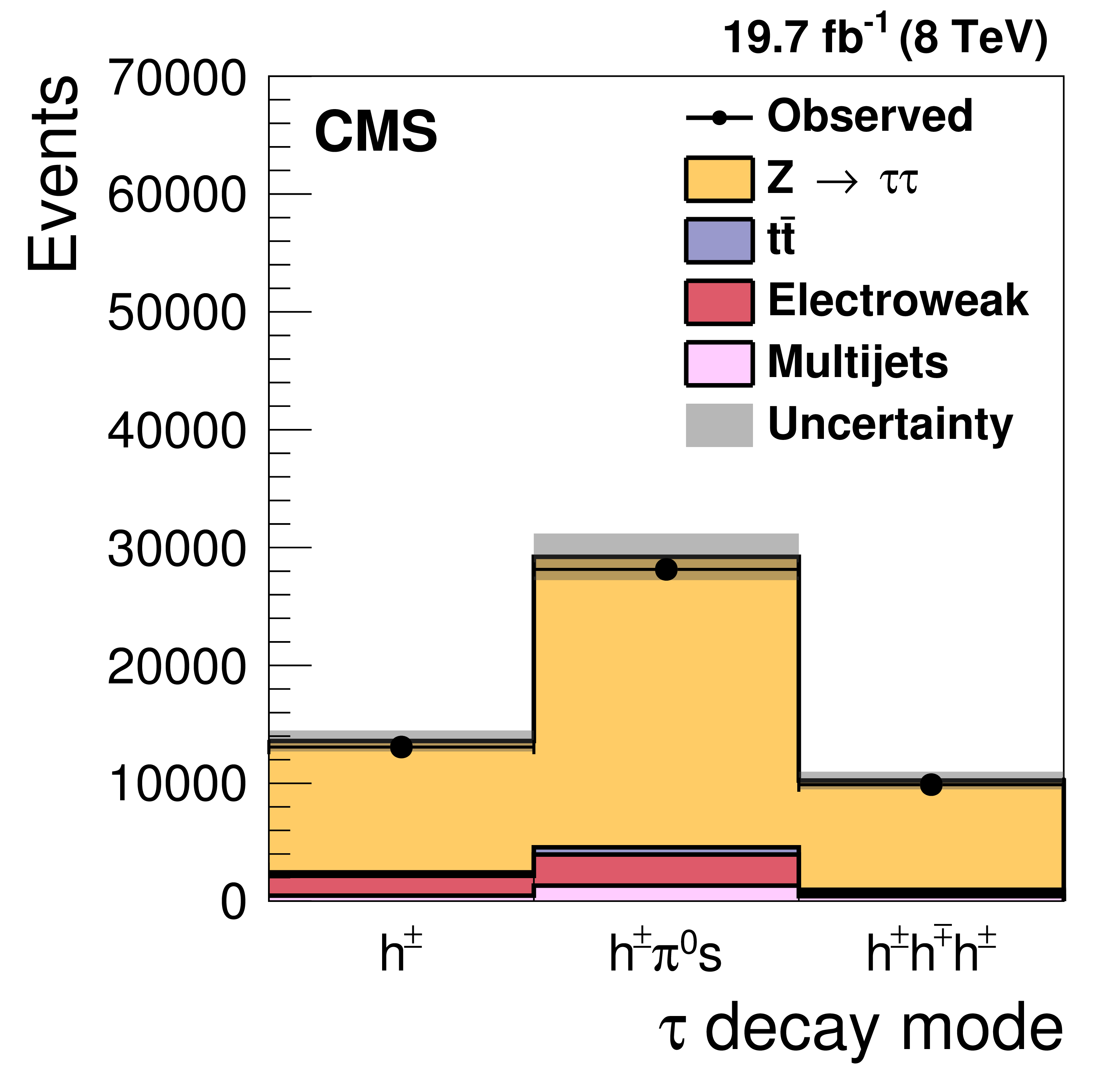
Figure 3-a:
Distributions in (a) reconstructed $ { {\tau }_{\mathrm {h}}} $ decay modes and (b) $ { {\tau }_{\mathrm {h}}} $ candidate masses in $ {\mathrm {Z}}/ { {\gamma } ^{*}} \to {\tau } {\tau }$ events selected in data, compared to MC expectations. The $ {\mathrm {Z}}/ { {\gamma } ^{*}} \to {\tau } {\tau }$ events are selected in the decay channel of muon and $ { {\tau }_{\mathrm {h}}} $, as described in Section 7.1.1. The $ { {\tau }_{\mathrm {h}}} $ are required to pass the medium working point of the MVA-based $ { {\tau }_{\mathrm {h}}} $ isolation discriminant. The mass of $ { {\tau }_{\mathrm {h}}} $ candidates reconstructed in simulated $ {\mathrm {Z}}/ { {\gamma } ^{*}} \to {\tau } {\tau }$ events is corrected for small data/MC differences in the $ { {\tau }_{\mathrm {h}}} $ energy scale, discussed in Section 9. The electroweak background is dominated by W+jets production, with minor contributions arising from single top quark and diboson production. The shaded uncertainty band represents the sum of systematic and statistical uncertainties on the MC simulation. |
png pdf |
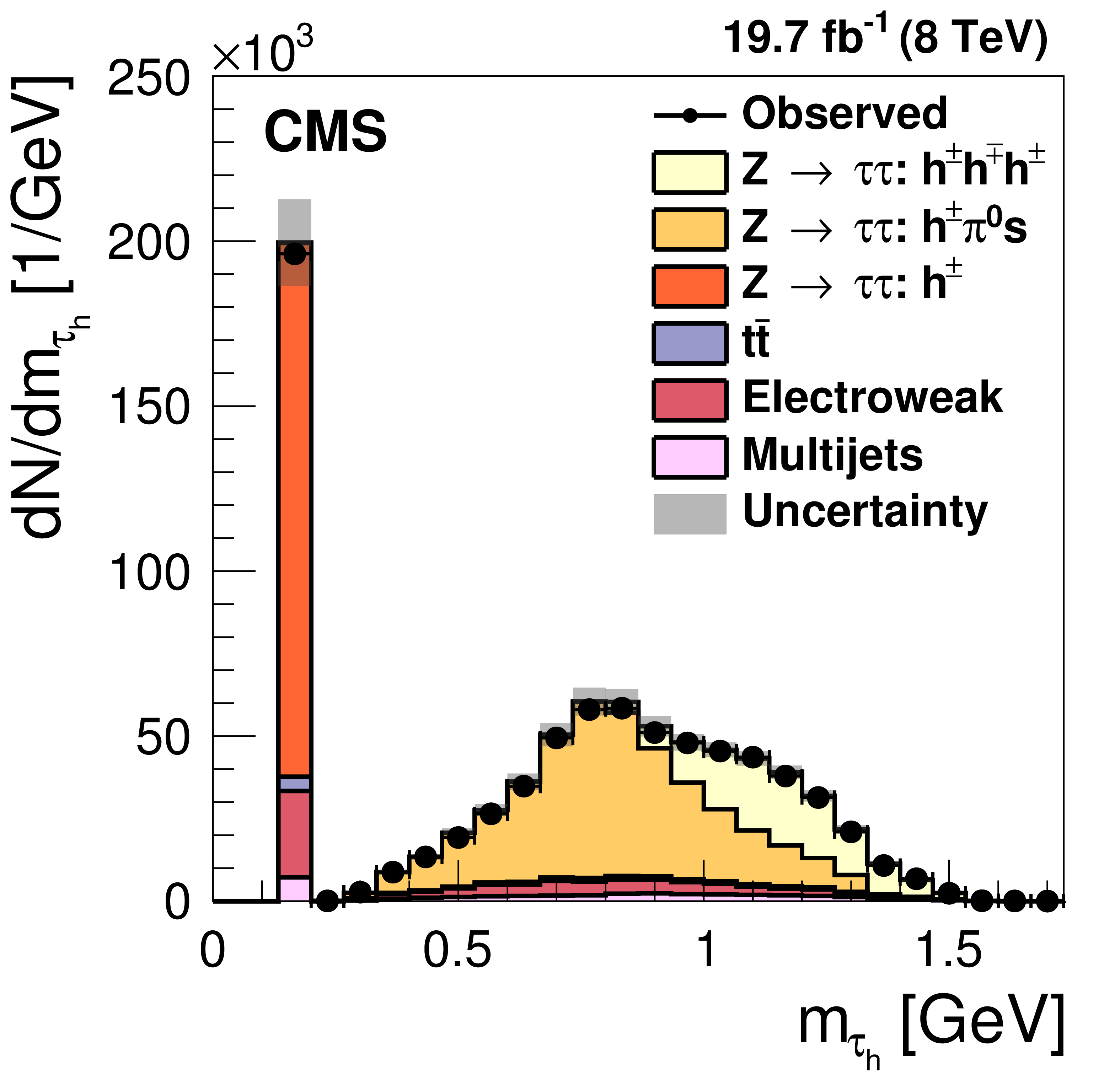
Figure 3-b:
Distributions in (a) reconstructed $ { {\tau }_{\mathrm {h}}} $ decay modes and (b) $ { {\tau }_{\mathrm {h}}} $ candidate masses in $ {\mathrm {Z}}/ { {\gamma } ^{*}} \to {\tau } {\tau }$ events selected in data, compared to MC expectations. The $ {\mathrm {Z}}/ { {\gamma } ^{*}} \to {\tau } {\tau }$ events are selected in the decay channel of muon and $ { {\tau }_{\mathrm {h}}} $, as described in Section 7.1.1. The $ { {\tau }_{\mathrm {h}}} $ are required to pass the medium working point of the MVA-based $ { {\tau }_{\mathrm {h}}} $ isolation discriminant. The mass of $ { {\tau }_{\mathrm {h}}} $ candidates reconstructed in simulated $ {\mathrm {Z}}/ { {\gamma } ^{*}} \to {\tau } {\tau }$ events is corrected for small data/MC differences in the $ { {\tau }_{\mathrm {h}}} $ energy scale, discussed in Section 9. The electroweak background is dominated by W+jets production, with minor contributions arising from single top quark and diboson production. The shaded uncertainty band represents the sum of systematic and statistical uncertainties on the MC simulation. |

png pdf |
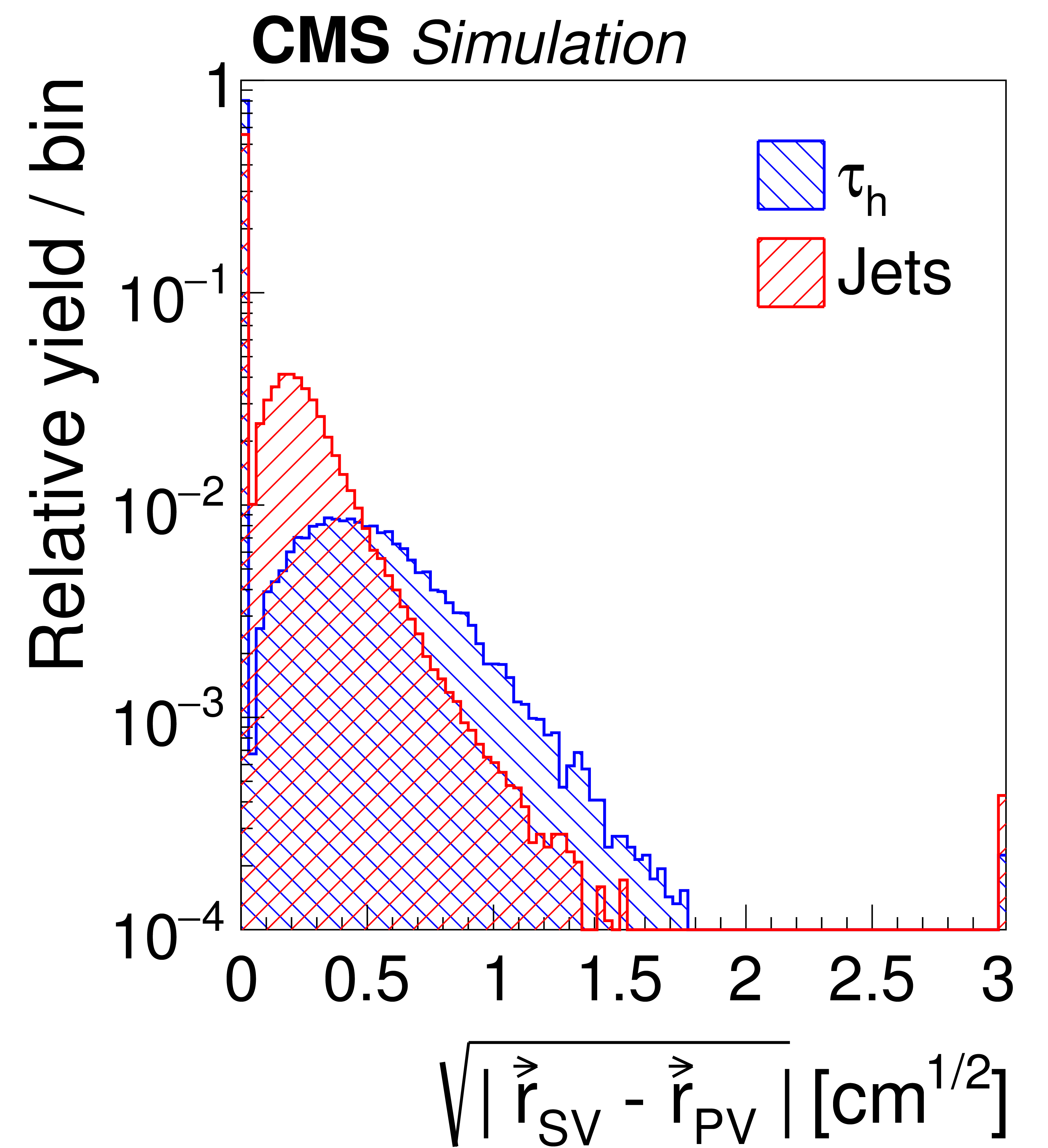
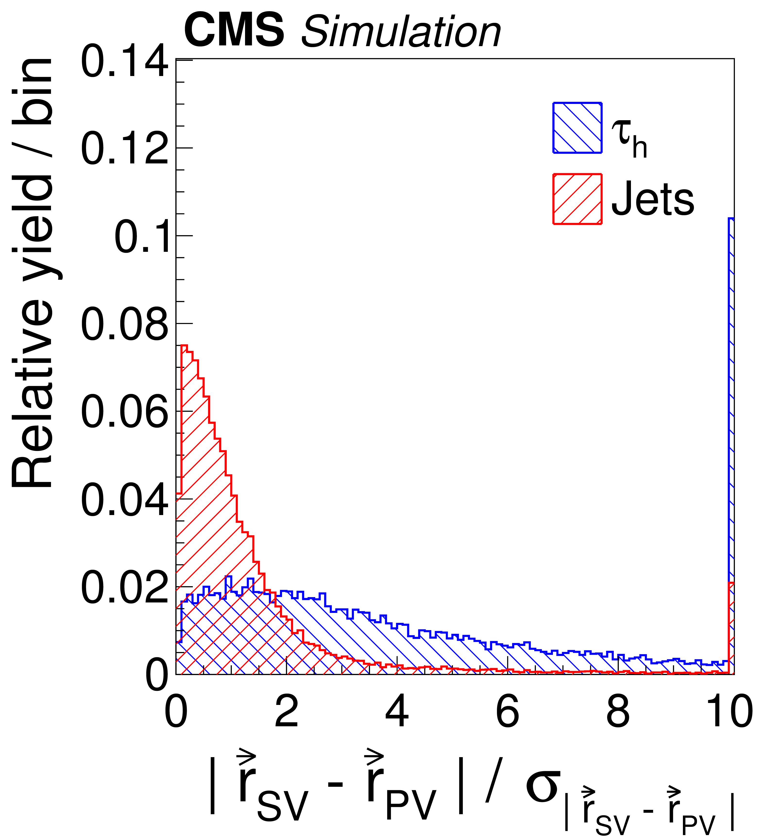
Figure 4-a:
Distributions, normalized to unity, in observables used as input variables to the MVA-based isolation discriminant, for hadronic $ {\tau }$ decays in simulated $ {\mathrm {Z}}/ { {\gamma } ^{*}} \to {\tau } {\tau }$ (blue), and jets in simulated W+jets (red) events. The $ { {\tau }_{\mathrm {h}}} $ candidates must have $ {p_{\mathrm {T}}} >$ 20 GeV and $ {| \eta | } <$ 2.3, and be reconstructed in one of the decay modes $ {\mathrm {h}^{\pm }} $, $ {\mathrm {h}^{\pm } { {\pi ^0}}} $, $ {\mathrm {h}^{\pm } { {\pi ^0}} { {\pi ^0}}} $, or $ {\mathrm {h}^{\pm }\mathrm {h}^{\mp }\mathrm {h}^{\pm }} $. In the plot (c) of the $ { {\tau }_{\mathrm {h}}} $ decay mode, an entry at 0 represents the decay mode $ {\mathrm {h}^{\pm }} $, 1 and 2 represent the decay modes $ {\mathrm {h}^{\pm } { {\pi ^0}}} $ and $ {\mathrm {h}^{\pm } { {\pi ^0}} { {\pi ^0}}} $, respectively, and entry 10 represents the $ {\mathrm {h}^{\pm }\mathrm {h}^{\mp }\mathrm {h}^{\pm }} $ decay mode. |
png pdf |
Figure 4-b:
Distributions, normalized to unity, in observables used as input variables to the MVA-based isolation discriminant, for hadronic $ {\tau }$ decays in simulated $ {\mathrm {Z}}/ { {\gamma } ^{*}} \to {\tau } {\tau }$ (blue), and jets in simulated W+jets (red) events. The $ { {\tau }_{\mathrm {h}}} $ candidates must have $ {p_{\mathrm {T}}} >$ 20 GeV and $ {| \eta | } <$ 2.3, and be reconstructed in one of the decay modes $ {\mathrm {h}^{\pm }} $, $ {\mathrm {h}^{\pm } { {\pi ^0}}} $, $ {\mathrm {h}^{\pm } { {\pi ^0}} { {\pi ^0}}} $, or $ {\mathrm {h}^{\pm }\mathrm {h}^{\mp }\mathrm {h}^{\pm }} $. In the plot (c) of the $ { {\tau }_{\mathrm {h}}} $ decay mode, an entry at 0 represents the decay mode $ {\mathrm {h}^{\pm }} $, 1 and 2 represent the decay modes $ {\mathrm {h}^{\pm } { {\pi ^0}}} $ and $ {\mathrm {h}^{\pm } { {\pi ^0}} { {\pi ^0}}} $, respectively, and entry 10 represents the $ {\mathrm {h}^{\pm }\mathrm {h}^{\mp }\mathrm {h}^{\pm }} $ decay mode. |
png pdf |
Figure 4-c:
Distributions, normalized to unity, in observables used as input variables to the MVA-based isolation discriminant, for hadronic $ {\tau }$ decays in simulated $ {\mathrm {Z}}/ { {\gamma } ^{*}} \to {\tau } {\tau }$ (blue), and jets in simulated W+jets (red) events. The $ { {\tau }_{\mathrm {h}}} $ candidates must have $ {p_{\mathrm {T}}} >$ 20 GeV and $ {| \eta | } <$ 2.3, and be reconstructed in one of the decay modes $ {\mathrm {h}^{\pm }} $, $ {\mathrm {h}^{\pm } { {\pi ^0}}} $, $ {\mathrm {h}^{\pm } { {\pi ^0}} { {\pi ^0}}} $, or $ {\mathrm {h}^{\pm }\mathrm {h}^{\mp }\mathrm {h}^{\pm }} $. In the plot (c) of the $ { {\tau }_{\mathrm {h}}} $ decay mode, an entry at 0 represents the decay mode $ {\mathrm {h}^{\pm }} $, 1 and 2 represent the decay modes $ {\mathrm {h}^{\pm } { {\pi ^0}}} $ and $ {\mathrm {h}^{\pm } { {\pi ^0}} { {\pi ^0}}} $, respectively, and entry 10 represents the $ {\mathrm {h}^{\pm }\mathrm {h}^{\mp }\mathrm {h}^{\pm }} $ decay mode. |

png pdf |
Figure 4-d:
Distributions, normalized to unity, in observables used as input variables to the MVA-based isolation discriminant, for hadronic $ {\tau }$ decays in simulated $ {\mathrm {Z}}/ { {\gamma } ^{*}} \to {\tau } {\tau }$ (blue), and jets in simulated W+jets (red) events. The $ { {\tau }_{\mathrm {h}}} $ candidates must have $ {p_{\mathrm {T}}} >$ 20 GeV and $ {| \eta | } <$ 2.3, and be reconstructed in one of the decay modes $ {\mathrm {h}^{\pm }} $, $ {\mathrm {h}^{\pm } { {\pi ^0}}} $, $ {\mathrm {h}^{\pm } { {\pi ^0}} { {\pi ^0}}} $, or $ {\mathrm {h}^{\pm }\mathrm {h}^{\mp }\mathrm {h}^{\pm }} $. In the plot (c) of the $ { {\tau }_{\mathrm {h}}} $ decay mode, an entry at 0 represents the decay mode $ {\mathrm {h}^{\pm }} $, 1 and 2 represent the decay modes $ {\mathrm {h}^{\pm } { {\pi ^0}}} $ and $ {\mathrm {h}^{\pm } { {\pi ^0}} { {\pi ^0}}} $, respectively, and entry 10 represents the $ {\mathrm {h}^{\pm }\mathrm {h}^{\mp }\mathrm {h}^{\pm }} $ decay mode. |

png pdf |
Figure 4-e:
Distributions, normalized to unity, in observables used as input variables to the MVA-based isolation discriminant, for hadronic $ {\tau }$ decays in simulated $ {\mathrm {Z}}/ { {\gamma } ^{*}} \to {\tau } {\tau }$ (blue), and jets in simulated W+jets (red) events. The $ { {\tau }_{\mathrm {h}}} $ candidates must have $ {p_{\mathrm {T}}} >$ 20 GeV and $ {| \eta | } <$ 2.3, and be reconstructed in one of the decay modes $ {\mathrm {h}^{\pm }} $, $ {\mathrm {h}^{\pm } { {\pi ^0}}} $, $ {\mathrm {h}^{\pm } { {\pi ^0}} { {\pi ^0}}} $, or $ {\mathrm {h}^{\pm }\mathrm {h}^{\mp }\mathrm {h}^{\pm }} $. In the plot (c) of the $ { {\tau }_{\mathrm {h}}} $ decay mode, an entry at 0 represents the decay mode $ {\mathrm {h}^{\pm }} $, 1 and 2 represent the decay modes $ {\mathrm {h}^{\pm } { {\pi ^0}}} $ and $ {\mathrm {h}^{\pm } { {\pi ^0}} { {\pi ^0}}} $, respectively, and entry 10 represents the $ {\mathrm {h}^{\pm }\mathrm {h}^{\mp }\mathrm {h}^{\pm }} $ decay mode. |
png pdf |
Figure 4-f:
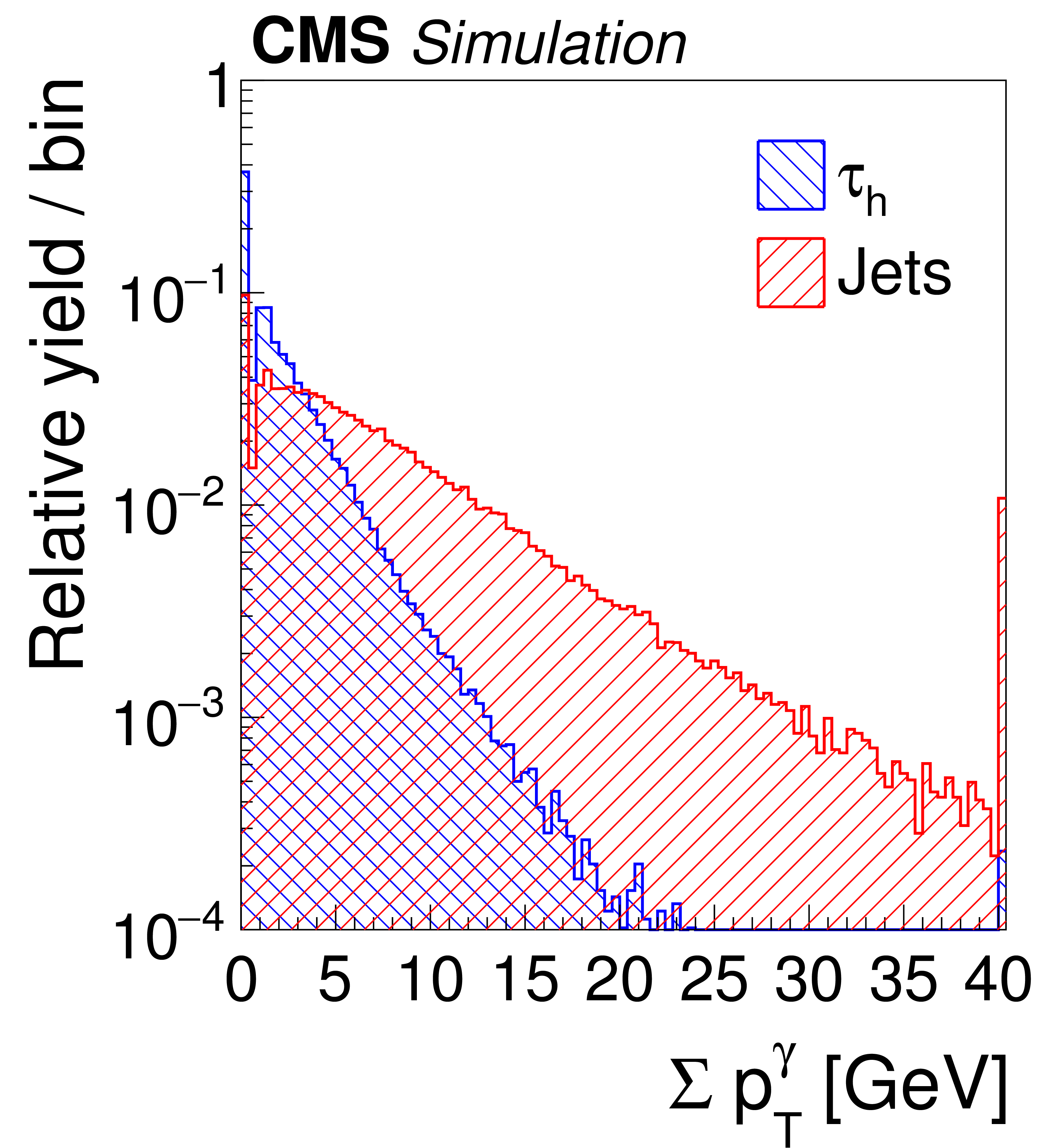
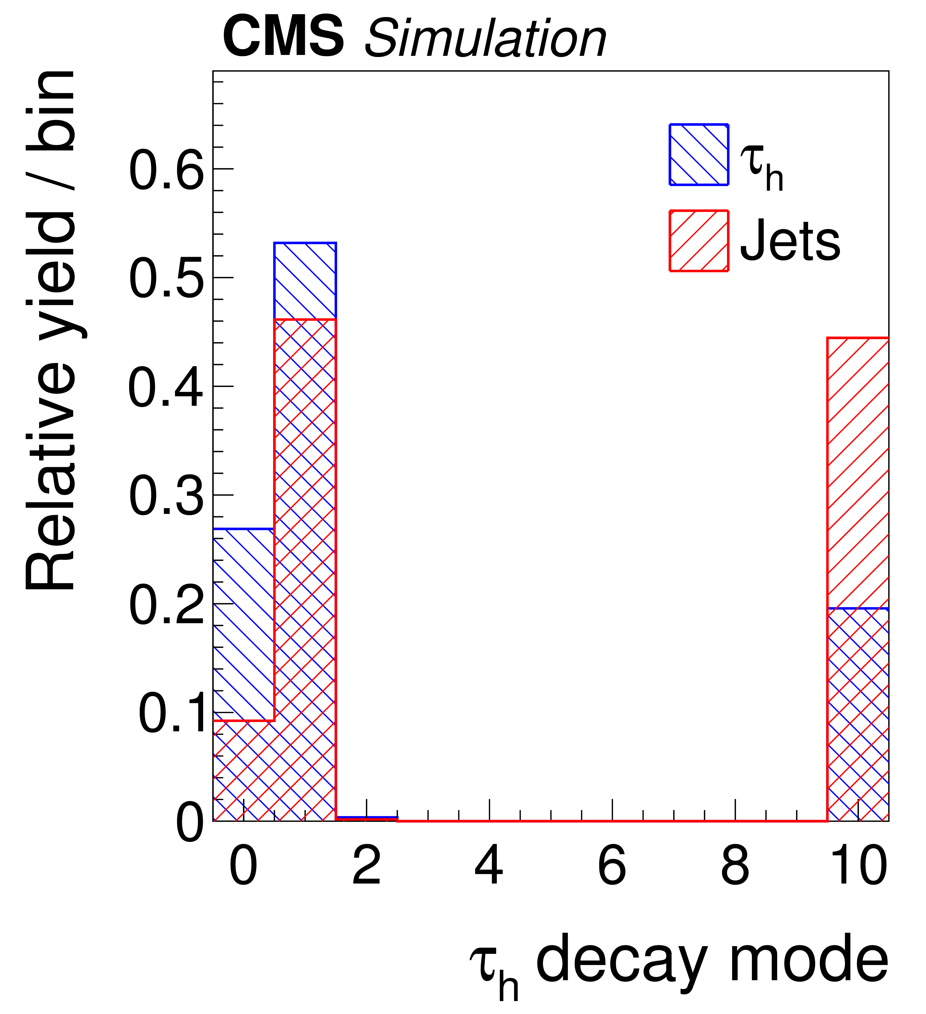
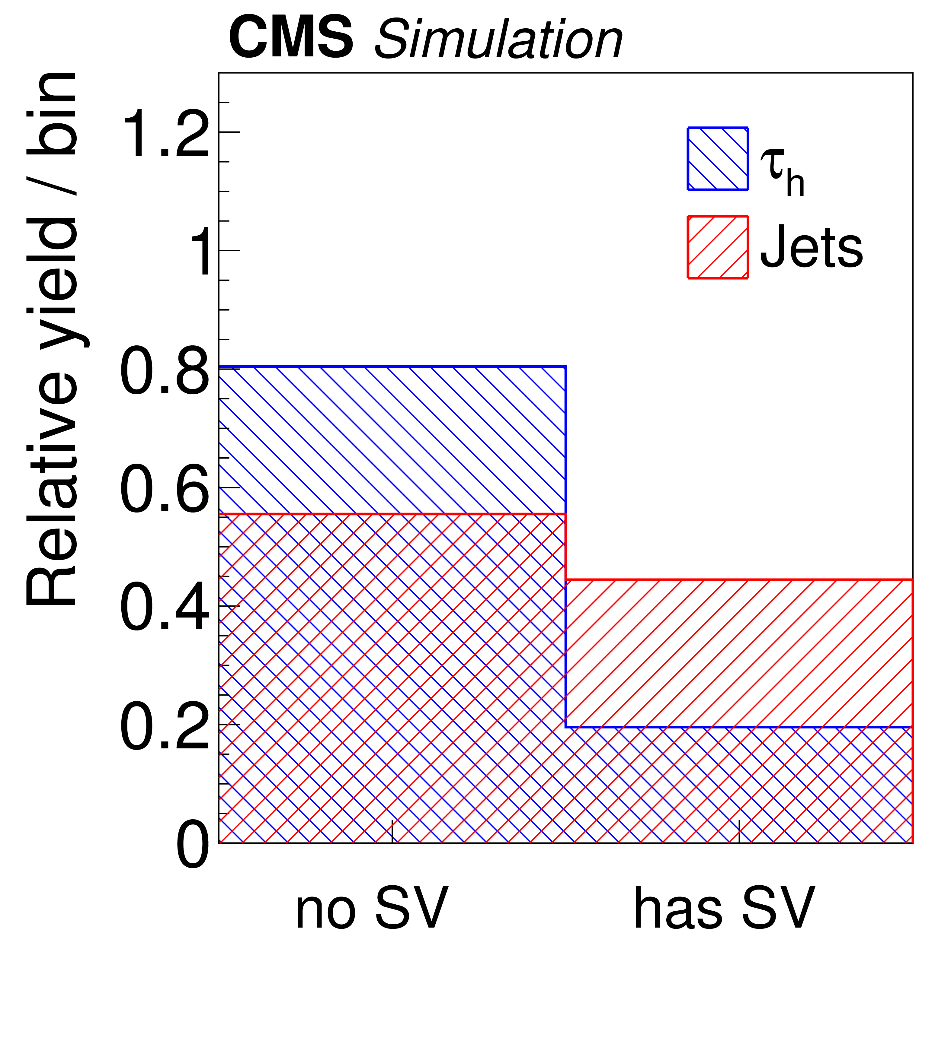
Distributions, normalized to unity, in observables used as input variables to the MVA-based isolation discriminant, for hadronic $ {\tau }$ decays in simulated $ {\mathrm {Z}}/ { {\gamma } ^{*}} \to {\tau } {\tau }$ (blue), and jets in simulated W+jets (red) events. The $ { {\tau }_{\mathrm {h}}} $ candidates must have $ {p_{\mathrm {T}}} >$ 20 GeV and $ {| \eta | } <$ 2.3, and be reconstructed in one of the decay modes $ {\mathrm {h}^{\pm }} $, $ {\mathrm {h}^{\pm } { {\pi ^0}}} $, $ {\mathrm {h}^{\pm } { {\pi ^0}} { {\pi ^0}}} $, or $ {\mathrm {h}^{\pm }\mathrm {h}^{\mp }\mathrm {h}^{\pm }} $. In the plot (c) of the $ { {\tau }_{\mathrm {h}}} $ decay mode, an entry at 0 represents the decay mode $ {\mathrm {h}^{\pm }} $, 1 and 2 represent the decay modes $ {\mathrm {h}^{\pm } { {\pi ^0}}} $ and $ {\mathrm {h}^{\pm } { {\pi ^0}} { {\pi ^0}}} $, respectively, and entry 10 represents the $ {\mathrm {h}^{\pm }\mathrm {h}^{\mp }\mathrm {h}^{\pm }} $ decay mode. |
png pdf |
Figure 4-g:
Distributions, normalized to unity, in observables used as input variables to the MVA-based isolation discriminant, for hadronic $ {\tau }$ decays in simulated $ {\mathrm {Z}}/ { {\gamma } ^{*}} \to {\tau } {\tau }$ (blue), and jets in simulated W+jets (red) events. The $ { {\tau }_{\mathrm {h}}} $ candidates must have $ {p_{\mathrm {T}}} >$ 20 GeV and $ {| \eta | } <$ 2.3, and be reconstructed in one of the decay modes $ {\mathrm {h}^{\pm }} $, $ {\mathrm {h}^{\pm } { {\pi ^0}}} $, $ {\mathrm {h}^{\pm } { {\pi ^0}} { {\pi ^0}}} $, or $ {\mathrm {h}^{\pm }\mathrm {h}^{\mp }\mathrm {h}^{\pm }} $. In the plot (c) of the $ { {\tau }_{\mathrm {h}}} $ decay mode, an entry at 0 represents the decay mode $ {\mathrm {h}^{\pm }} $, 1 and 2 represent the decay modes $ {\mathrm {h}^{\pm } { {\pi ^0}}} $ and $ {\mathrm {h}^{\pm } { {\pi ^0}} { {\pi ^0}}} $, respectively, and entry 10 represents the $ {\mathrm {h}^{\pm }\mathrm {h}^{\mp }\mathrm {h}^{\pm }} $ decay mode. |
png pdf |
Figure 4-h:
Distributions, normalized to unity, in observables used as input variables to the MVA-based isolation discriminant, for hadronic $ {\tau }$ decays in simulated $ {\mathrm {Z}}/ { {\gamma } ^{*}} \to {\tau } {\tau }$ (blue), and jets in simulated W+jets (red) events. The $ { {\tau }_{\mathrm {h}}} $ candidates must have $ {p_{\mathrm {T}}} >$ 20 GeV and $ {| \eta | } <$ 2.3, and be reconstructed in one of the decay modes $ {\mathrm {h}^{\pm }} $, $ {\mathrm {h}^{\pm } { {\pi ^0}}} $, $ {\mathrm {h}^{\pm } { {\pi ^0}} { {\pi ^0}}} $, or $ {\mathrm {h}^{\pm }\mathrm {h}^{\mp }\mathrm {h}^{\pm }} $. In the plot (c) of the $ { {\tau }_{\mathrm {h}}} $ decay mode, an entry at 0 represents the decay mode $ {\mathrm {h}^{\pm }} $, 1 and 2 represent the decay modes $ {\mathrm {h}^{\pm } { {\pi ^0}}} $ and $ {\mathrm {h}^{\pm } { {\pi ^0}} { {\pi ^0}}} $, respectively, and entry 10 represents the $ {\mathrm {h}^{\pm }\mathrm {h}^{\mp }\mathrm {h}^{\pm }} $ decay mode. |

png pdf |
Figure 5:
Distribution of MVA output for the $ { {\tau }_{\mathrm {h}}} $ identification discriminant that includes lifetime information for hadronic $ {\tau }$ decays in simulated $ {\mathrm {Z}}/ { {\gamma } ^{*}} \to {\tau } {\tau }$ (blue), and jets in simulated W+jets (red) events. |
png pdf |
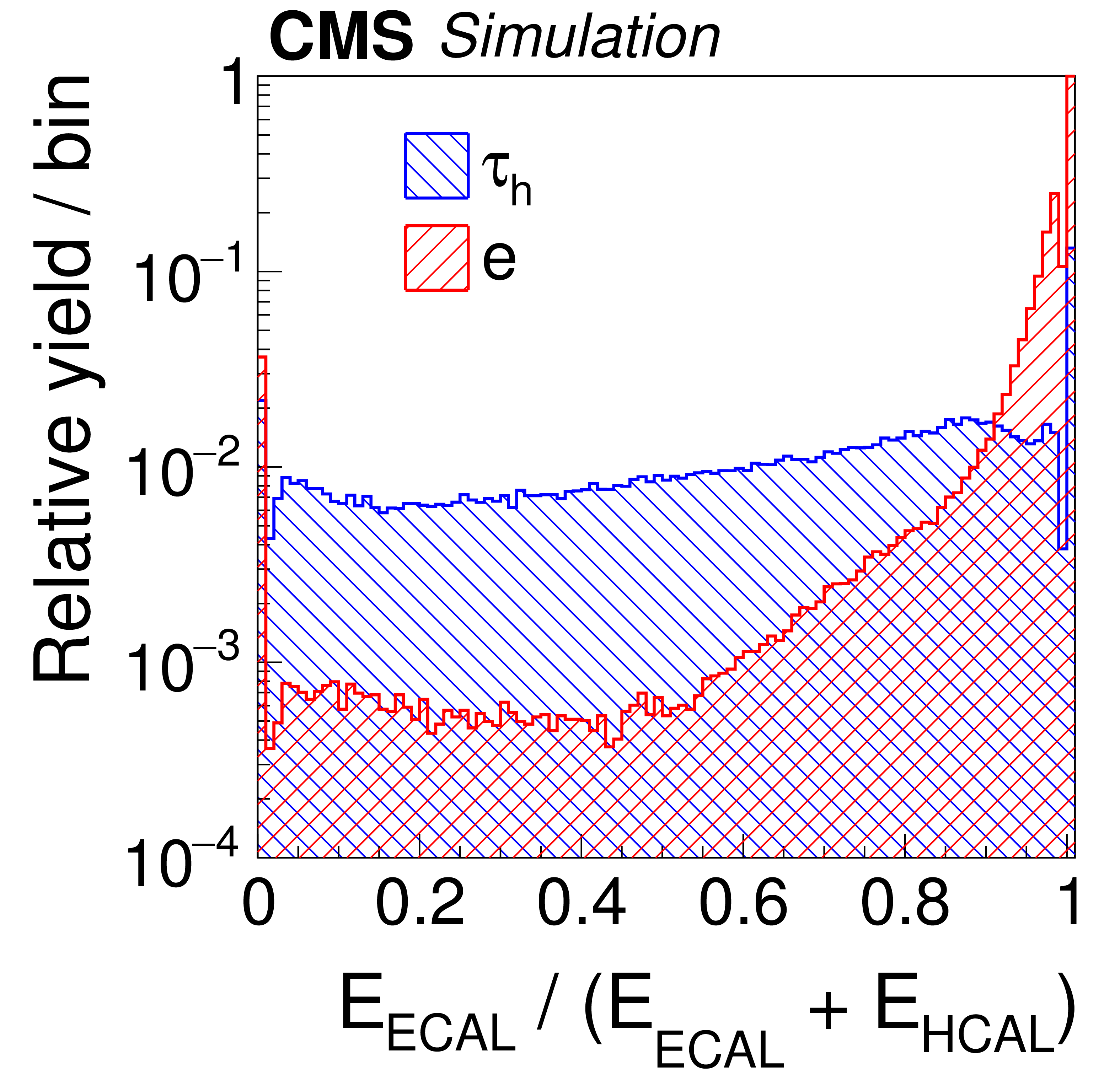
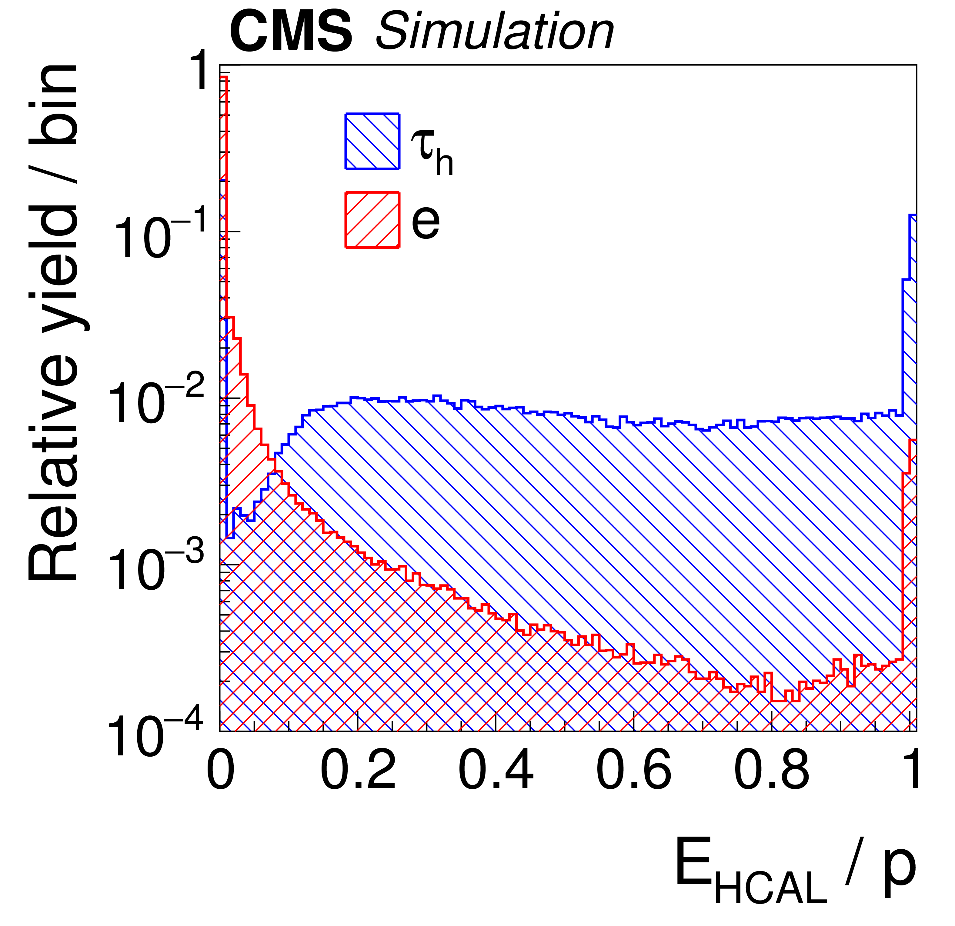
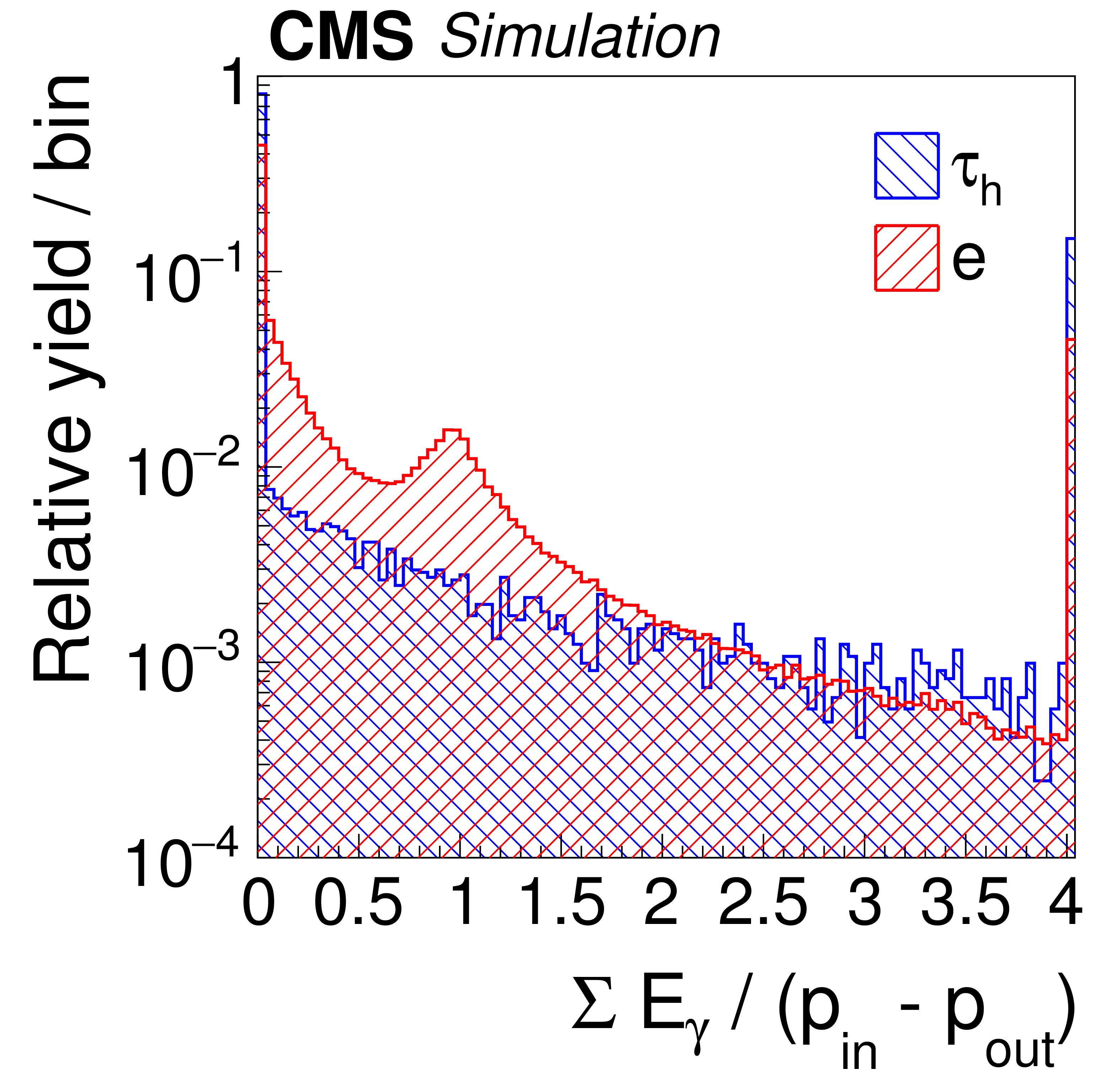
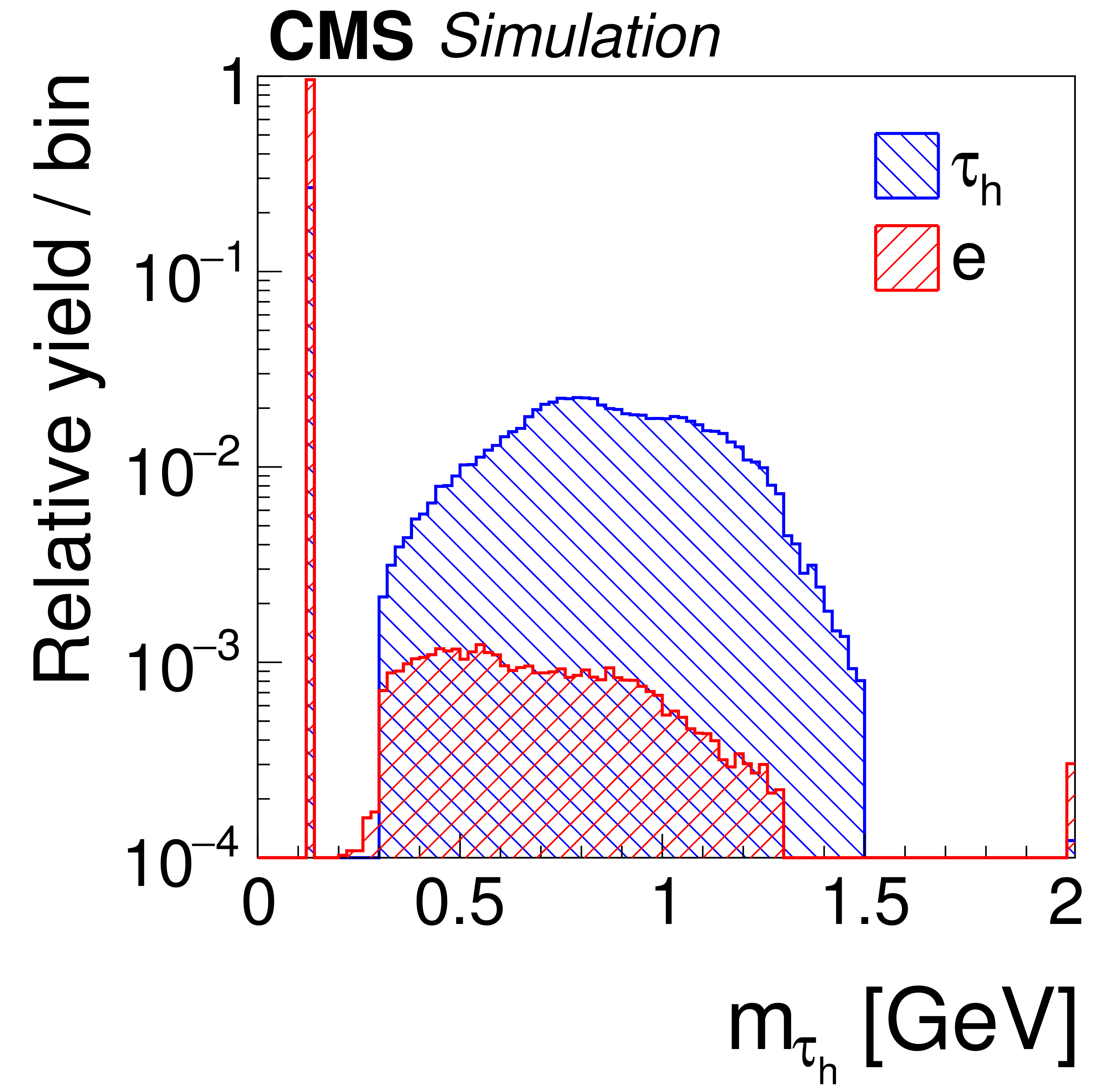
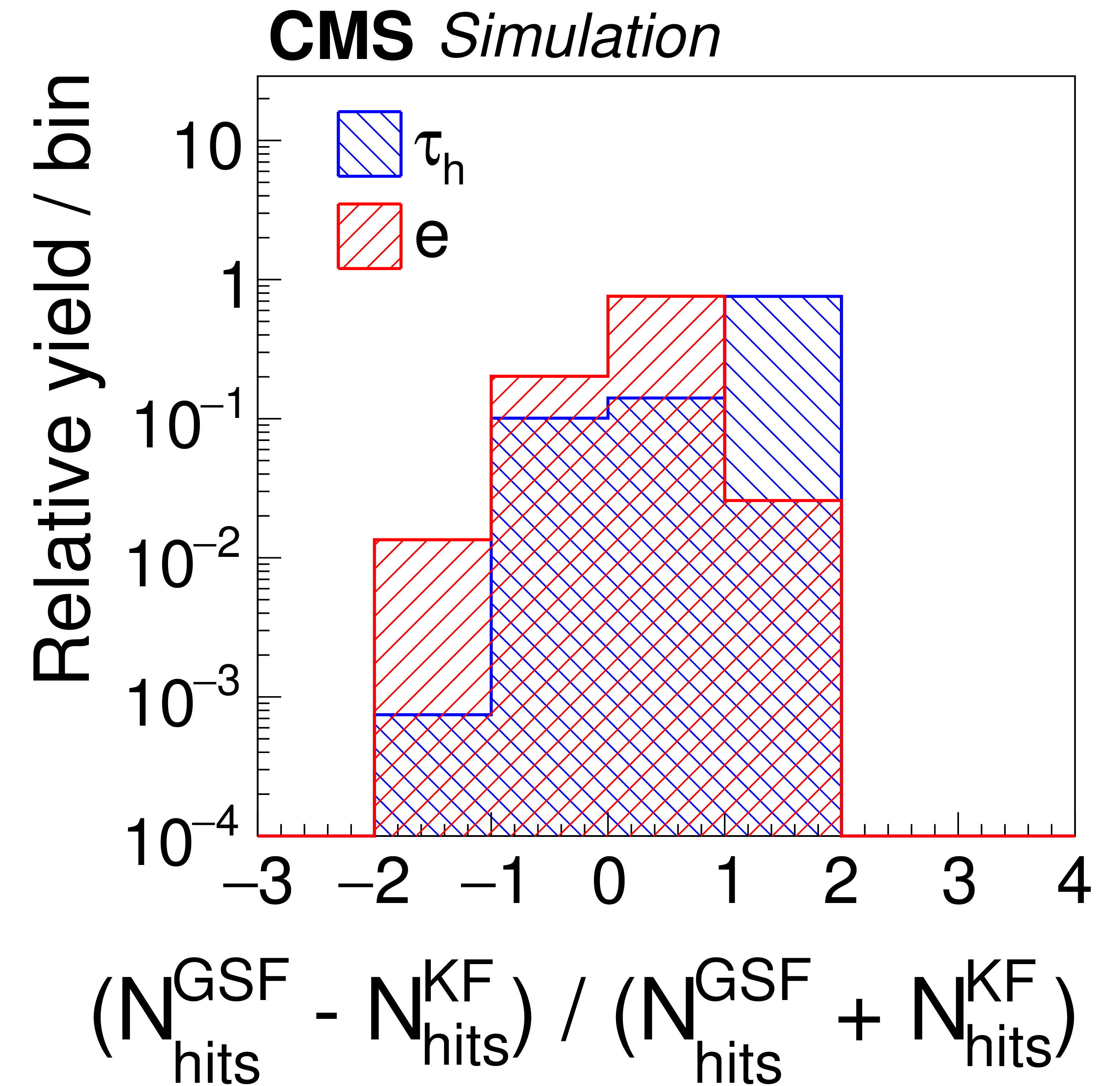
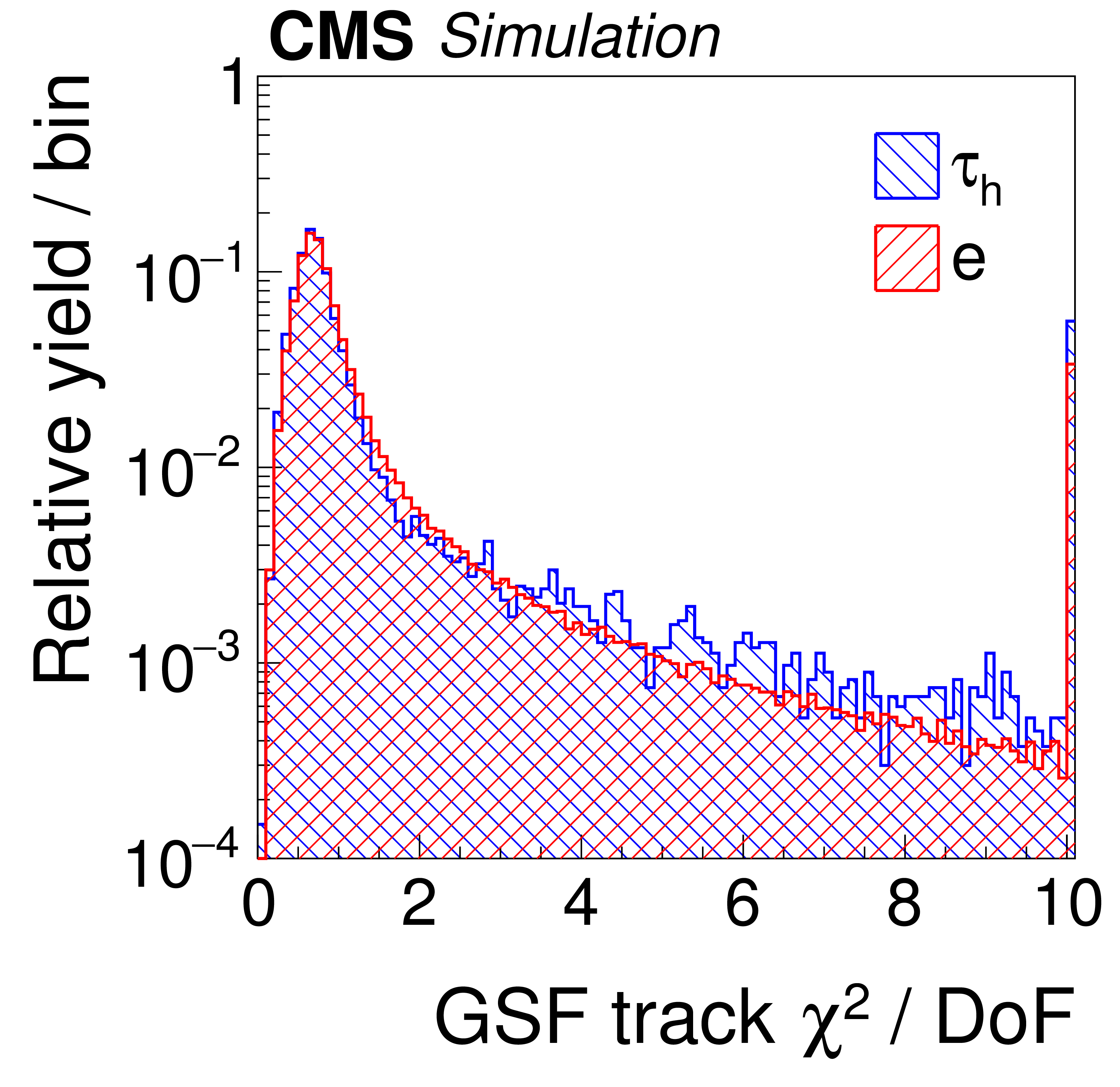
Figure 6-a:
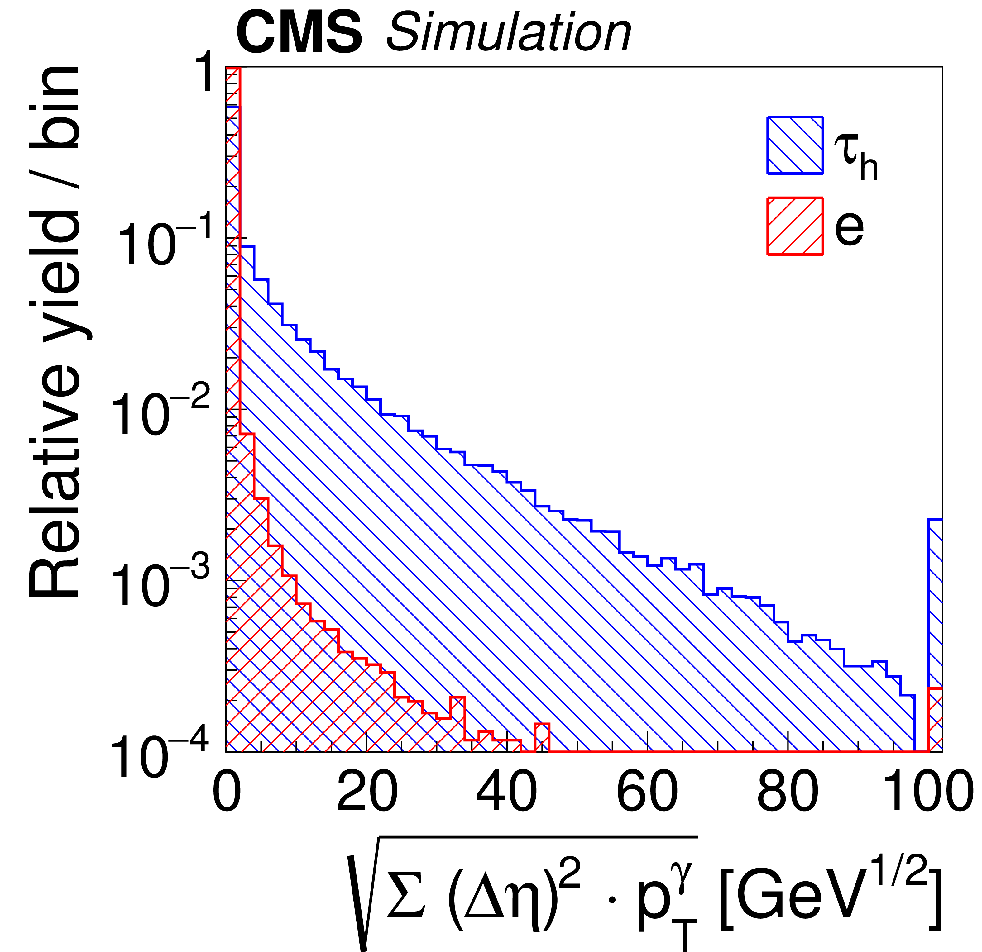
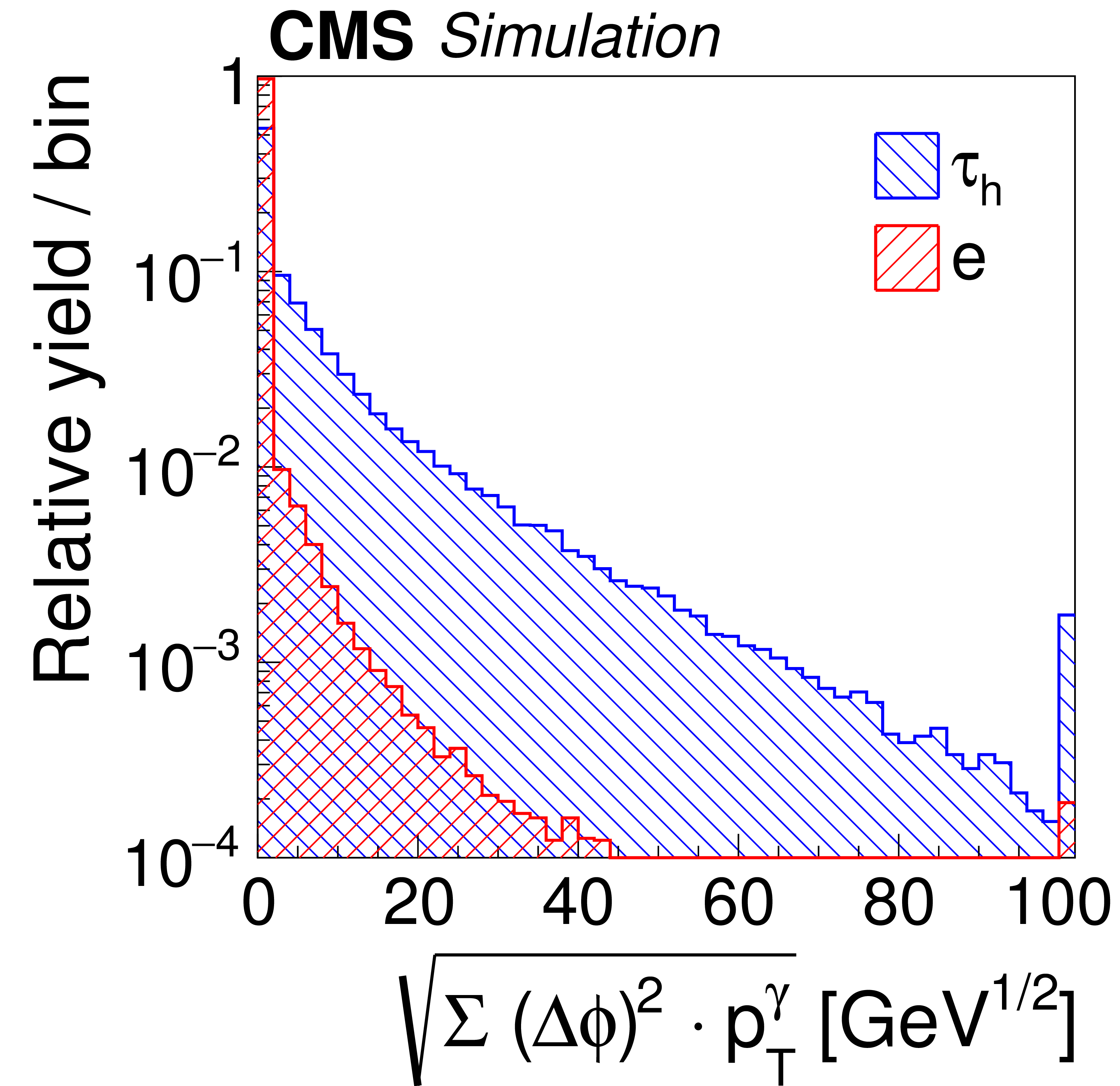
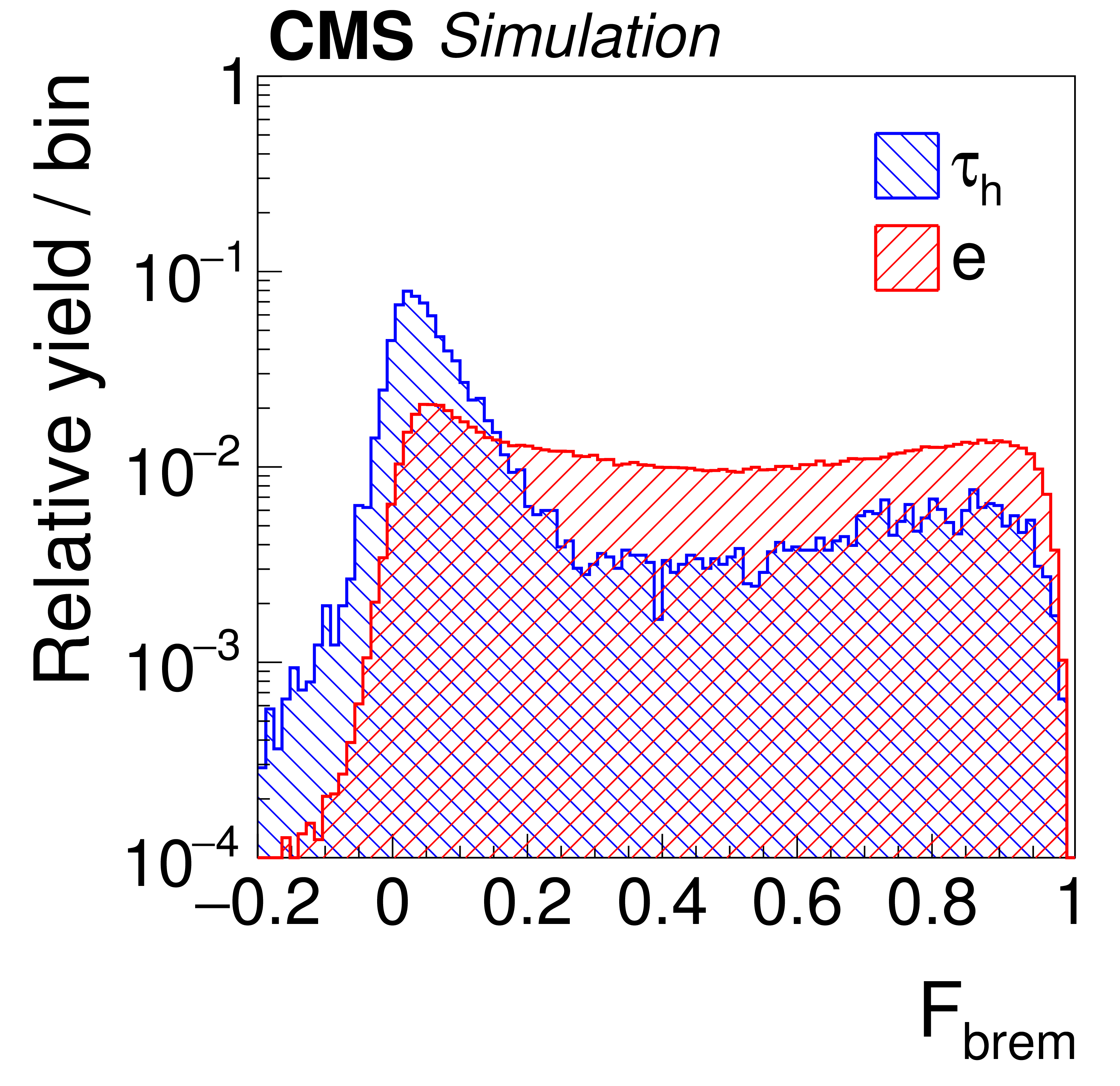
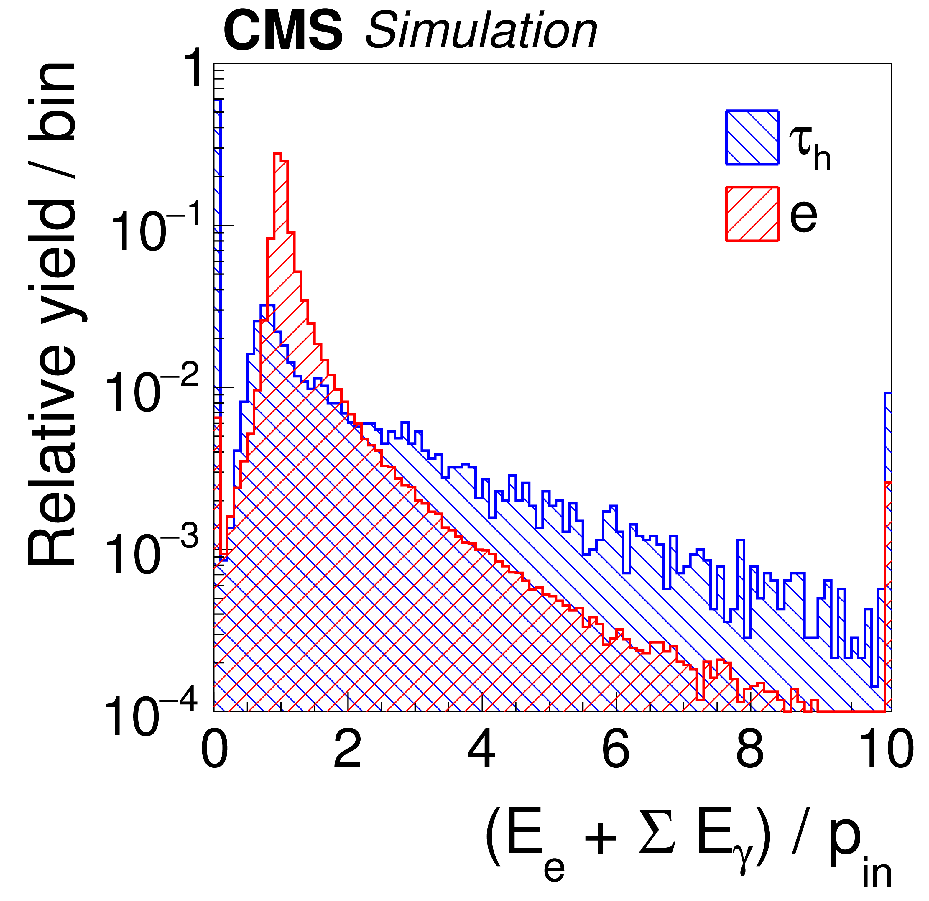
Distributions, normalized to unity, in observables that are used as inputs to the MVA-based electron discriminant, for hadronic $ {\tau }$ decays in simulated $ {\mathrm {Z}}/ { {\gamma } ^{*}} \to {\tau } {\tau }$ (blue), and electrons in simulated $ {\mathrm {Z}}/ { {\gamma } ^{*}} \to {\mathrm {e}} {\mathrm {e}}$ (red) events. The $ { {\tau }_{\mathrm {h}}} $ candidates must have $ {p_{\mathrm {T}}} >$ 20 GeV and $ {| \eta | } <$ 2.3, and be reconstructed in one of the decay modes $ {\mathrm {h}^{\pm }} $, $ {\mathrm {h}^{\pm } { {\pi ^0}}} $, $ {\mathrm {h}^{\pm } { {\pi ^0}} { {\pi ^0}}} $, or $ {\mathrm {h}^{\pm }\mathrm {h}^{\mp }\mathrm {h}^{\pm }} $. |

png pdf |
Figure 6-b:
Distributions, normalized to unity, in observables that are used as inputs to the MVA-based electron discriminant, for hadronic $ {\tau }$ decays in simulated $ {\mathrm {Z}}/ { {\gamma } ^{*}} \to {\tau } {\tau }$ (blue), and electrons in simulated $ {\mathrm {Z}}/ { {\gamma } ^{*}} \to {\mathrm {e}} {\mathrm {e}}$ (red) events. The $ { {\tau }_{\mathrm {h}}} $ candidates must have $ {p_{\mathrm {T}}} >$ 20 GeV and $ {| \eta | } <$ 2.3, and be reconstructed in one of the decay modes $ {\mathrm {h}^{\pm }} $, $ {\mathrm {h}^{\pm } { {\pi ^0}}} $, $ {\mathrm {h}^{\pm } { {\pi ^0}} { {\pi ^0}}} $, or $ {\mathrm {h}^{\pm }\mathrm {h}^{\mp }\mathrm {h}^{\pm }} $. |
png pdf |
Figure 6-c:
Distributions, normalized to unity, in observables that are used as inputs to the MVA-based electron discriminant, for hadronic $ {\tau }$ decays in simulated $ {\mathrm {Z}}/ { {\gamma } ^{*}} \to {\tau } {\tau }$ (blue), and electrons in simulated $ {\mathrm {Z}}/ { {\gamma } ^{*}} \to {\mathrm {e}} {\mathrm {e}}$ (red) events. The $ { {\tau }_{\mathrm {h}}} $ candidates must have $ {p_{\mathrm {T}}} >$ 20 GeV and $ {| \eta | } <$ 2.3, and be reconstructed in one of the decay modes $ {\mathrm {h}^{\pm }} $, $ {\mathrm {h}^{\pm } { {\pi ^0}}} $, $ {\mathrm {h}^{\pm } { {\pi ^0}} { {\pi ^0}}} $, or $ {\mathrm {h}^{\pm }\mathrm {h}^{\mp }\mathrm {h}^{\pm }} $. |
png pdf |
Figure 6-d:
Distributions, normalized to unity, in observables that are used as inputs to the MVA-based electron discriminant, for hadronic $ {\tau }$ decays in simulated $ {\mathrm {Z}}/ { {\gamma } ^{*}} \to {\tau } {\tau }$ (blue), and electrons in simulated $ {\mathrm {Z}}/ { {\gamma } ^{*}} \to {\mathrm {e}} {\mathrm {e}}$ (red) events. The $ { {\tau }_{\mathrm {h}}} $ candidates must have $ {p_{\mathrm {T}}} >$ 20 GeV and $ {| \eta | } <$ 2.3, and be reconstructed in one of the decay modes $ {\mathrm {h}^{\pm }} $, $ {\mathrm {h}^{\pm } { {\pi ^0}}} $, $ {\mathrm {h}^{\pm } { {\pi ^0}} { {\pi ^0}}} $, or $ {\mathrm {h}^{\pm }\mathrm {h}^{\mp }\mathrm {h}^{\pm }} $. |
png pdf |
Figure 6-e:
Distributions, normalized to unity, in observables that are used as inputs to the MVA-based electron discriminant, for hadronic $ {\tau }$ decays in simulated $ {\mathrm {Z}}/ { {\gamma } ^{*}} \to {\tau } {\tau }$ (blue), and electrons in simulated $ {\mathrm {Z}}/ { {\gamma } ^{*}} \to {\mathrm {e}} {\mathrm {e}}$ (red) events. The $ { {\tau }_{\mathrm {h}}} $ candidates must have $ {p_{\mathrm {T}}} >$ 20 GeV and $ {| \eta | } <$ 2.3, and be reconstructed in one of the decay modes $ {\mathrm {h}^{\pm }} $, $ {\mathrm {h}^{\pm } { {\pi ^0}}} $, $ {\mathrm {h}^{\pm } { {\pi ^0}} { {\pi ^0}}} $, or $ {\mathrm {h}^{\pm }\mathrm {h}^{\mp }\mathrm {h}^{\pm }} $. |

png pdf |
Figure 6-f:
Distributions, normalized to unity, in observables that are used as inputs to the MVA-based electron discriminant, for hadronic $ {\tau }$ decays in simulated $ {\mathrm {Z}}/ { {\gamma } ^{*}} \to {\tau } {\tau }$ (blue), and electrons in simulated $ {\mathrm {Z}}/ { {\gamma } ^{*}} \to {\mathrm {e}} {\mathrm {e}}$ (red) events. The $ { {\tau }_{\mathrm {h}}} $ candidates must have $ {p_{\mathrm {T}}} >$ 20 GeV and $ {| \eta | } <$ 2.3, and be reconstructed in one of the decay modes $ {\mathrm {h}^{\pm }} $, $ {\mathrm {h}^{\pm } { {\pi ^0}}} $, $ {\mathrm {h}^{\pm } { {\pi ^0}} { {\pi ^0}}} $, or $ {\mathrm {h}^{\pm }\mathrm {h}^{\mp }\mathrm {h}^{\pm }} $. |
png pdf |
Figure 6-g:
Distributions, normalized to unity, in observables that are used as inputs to the MVA-based electron discriminant, for hadronic $ {\tau }$ decays in simulated $ {\mathrm {Z}}/ { {\gamma } ^{*}} \to {\tau } {\tau }$ (blue), and electrons in simulated $ {\mathrm {Z}}/ { {\gamma } ^{*}} \to {\mathrm {e}} {\mathrm {e}}$ (red) events. The $ { {\tau }_{\mathrm {h}}} $ candidates must have $ {p_{\mathrm {T}}} >$ 20 GeV and $ {| \eta | } <$ 2.3, and be reconstructed in one of the decay modes $ {\mathrm {h}^{\pm }} $, $ {\mathrm {h}^{\pm } { {\pi ^0}}} $, $ {\mathrm {h}^{\pm } { {\pi ^0}} { {\pi ^0}}} $, or $ {\mathrm {h}^{\pm }\mathrm {h}^{\mp }\mathrm {h}^{\pm }} $. |
png pdf |
Figure 6-h:
Distributions, normalized to unity, in observables that are used as inputs to the MVA-based electron discriminant, for hadronic $ {\tau }$ decays in simulated $ {\mathrm {Z}}/ { {\gamma } ^{*}} \to {\tau } {\tau }$ (blue), and electrons in simulated $ {\mathrm {Z}}/ { {\gamma } ^{*}} \to {\mathrm {e}} {\mathrm {e}}$ (red) events. The $ { {\tau }_{\mathrm {h}}} $ candidates must have $ {p_{\mathrm {T}}} >$ 20 GeV and $ {| \eta | } <$ 2.3, and be reconstructed in one of the decay modes $ {\mathrm {h}^{\pm }} $, $ {\mathrm {h}^{\pm } { {\pi ^0}}} $, $ {\mathrm {h}^{\pm } { {\pi ^0}} { {\pi ^0}}} $, or $ {\mathrm {h}^{\pm }\mathrm {h}^{\mp }\mathrm {h}^{\pm }} $. |
png pdf |
Figure 6-i:
Distributions, normalized to unity, in observables that are used as inputs to the MVA-based electron discriminant, for hadronic $ {\tau }$ decays in simulated $ {\mathrm {Z}}/ { {\gamma } ^{*}} \to {\tau } {\tau }$ (blue), and electrons in simulated $ {\mathrm {Z}}/ { {\gamma } ^{*}} \to {\mathrm {e}} {\mathrm {e}}$ (red) events. The $ { {\tau }_{\mathrm {h}}} $ candidates must have $ {p_{\mathrm {T}}} >$ 20 GeV and $ {| \eta | } <$ 2.3, and be reconstructed in one of the decay modes $ {\mathrm {h}^{\pm }} $, $ {\mathrm {h}^{\pm } { {\pi ^0}}} $, $ {\mathrm {h}^{\pm } { {\pi ^0}} { {\pi ^0}}} $, or $ {\mathrm {h}^{\pm }\mathrm {h}^{\mp }\mathrm {h}^{\pm }} $. |
png pdf |
Figure 6-j:
Distributions, normalized to unity, in observables that are used as inputs to the MVA-based electron discriminant, for hadronic $ {\tau }$ decays in simulated $ {\mathrm {Z}}/ { {\gamma } ^{*}} \to {\tau } {\tau }$ (blue), and electrons in simulated $ {\mathrm {Z}}/ { {\gamma } ^{*}} \to {\mathrm {e}} {\mathrm {e}}$ (red) events. The $ { {\tau }_{\mathrm {h}}} $ candidates must have $ {p_{\mathrm {T}}} >$ 20 GeV and $ {| \eta | } <$ 2.3, and be reconstructed in one of the decay modes $ {\mathrm {h}^{\pm }} $, $ {\mathrm {h}^{\pm } { {\pi ^0}}} $, $ {\mathrm {h}^{\pm } { {\pi ^0}} { {\pi ^0}}} $, or $ {\mathrm {h}^{\pm }\mathrm {h}^{\mp }\mathrm {h}^{\pm }} $. |
png pdf |
Figure 6-k:
Distributions, normalized to unity, in observables that are used as inputs to the MVA-based electron discriminant, for hadronic $ {\tau }$ decays in simulated $ {\mathrm {Z}}/ { {\gamma } ^{*}} \to {\tau } {\tau }$ (blue), and electrons in simulated $ {\mathrm {Z}}/ { {\gamma } ^{*}} \to {\mathrm {e}} {\mathrm {e}}$ (red) events. The $ { {\tau }_{\mathrm {h}}} $ candidates must have $ {p_{\mathrm {T}}} >$ 20 GeV and $ {| \eta | } <$ 2.3, and be reconstructed in one of the decay modes $ {\mathrm {h}^{\pm }} $, $ {\mathrm {h}^{\pm } { {\pi ^0}}} $, $ {\mathrm {h}^{\pm } { {\pi ^0}} { {\pi ^0}}} $, or $ {\mathrm {h}^{\pm }\mathrm {h}^{\mp }\mathrm {h}^{\pm }} $. |
png pdf |
Figure 6-l:
Distributions, normalized to unity, in observables that are used as inputs to the MVA-based electron discriminant, for hadronic $ {\tau }$ decays in simulated $ {\mathrm {Z}}/ { {\gamma } ^{*}} \to {\tau } {\tau }$ (blue), and electrons in simulated $ {\mathrm {Z}}/ { {\gamma } ^{*}} \to {\mathrm {e}} {\mathrm {e}}$ (red) events. The $ { {\tau }_{\mathrm {h}}} $ candidates must have $ {p_{\mathrm {T}}} >$ 20 GeV and $ {| \eta | } <$ 2.3, and be reconstructed in one of the decay modes $ {\mathrm {h}^{\pm }} $, $ {\mathrm {h}^{\pm } { {\pi ^0}}} $, $ {\mathrm {h}^{\pm } { {\pi ^0}} { {\pi ^0}}} $, or $ {\mathrm {h}^{\pm }\mathrm {h}^{\mp }\mathrm {h}^{\pm }} $. |
png pdf |
Figure 7-a:
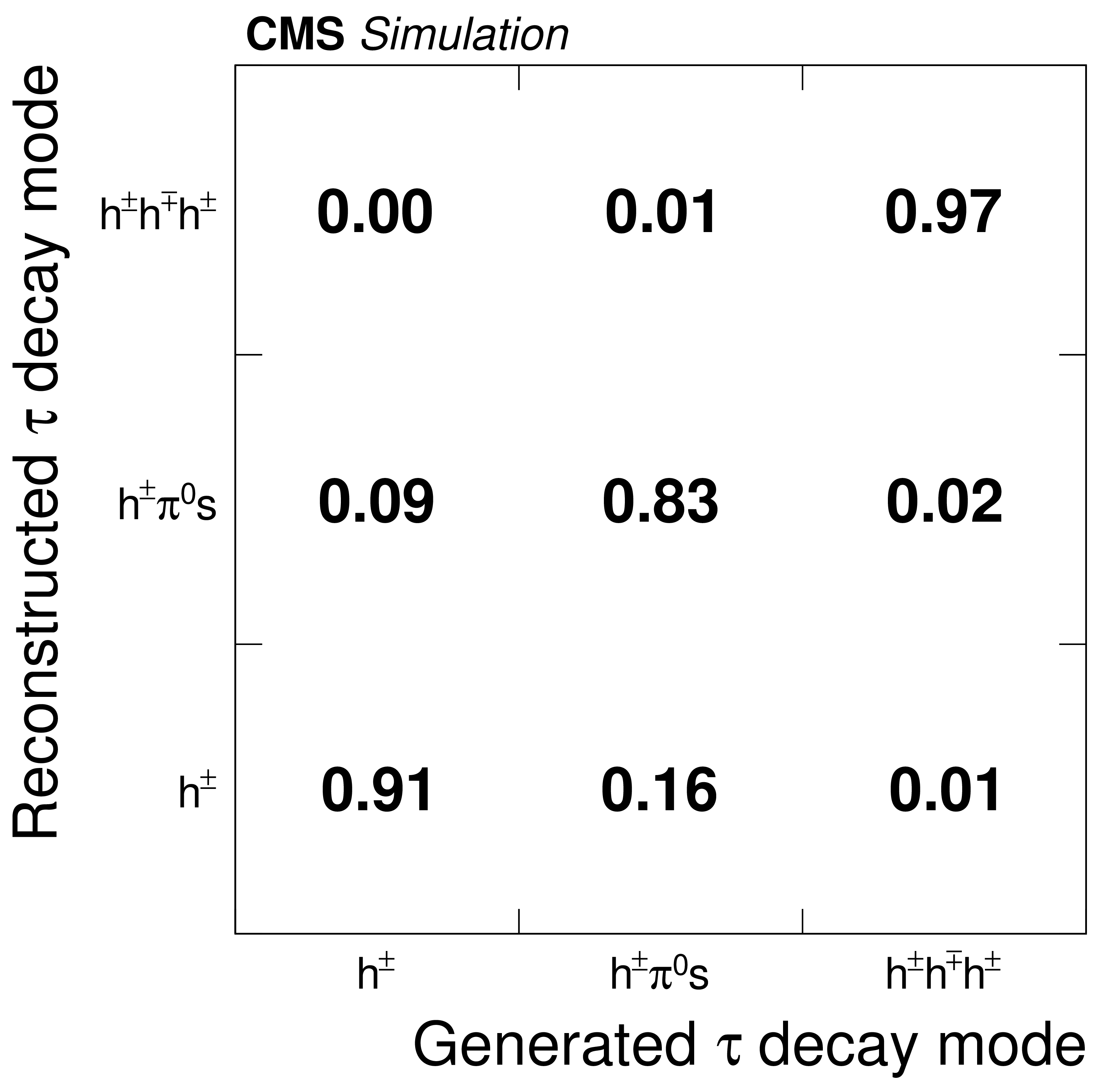
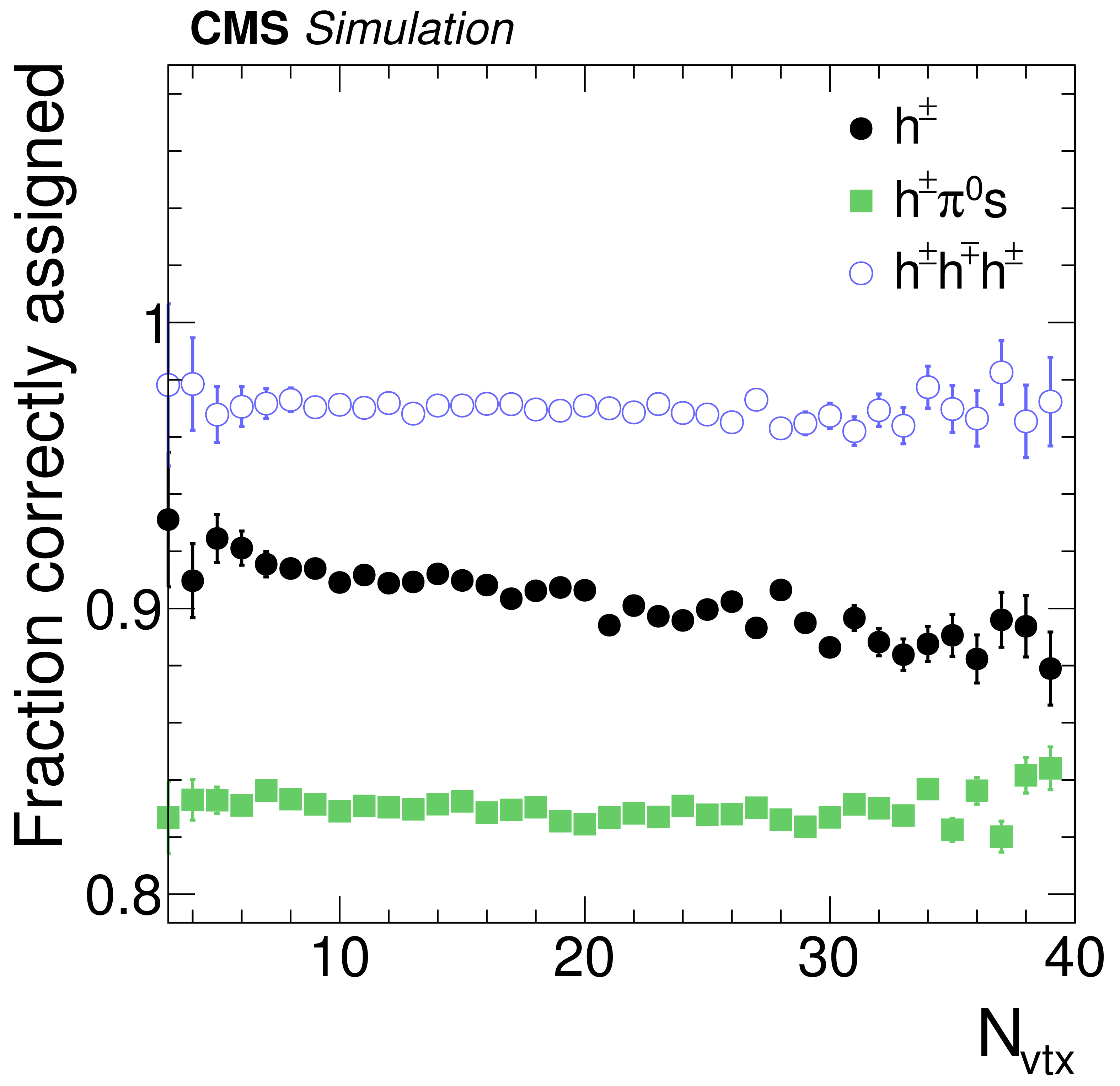
a: Correlation between generated and reconstructed $ { {\tau }_{\mathrm {h}}} $ decay modes for $ { {\tau }_{\mathrm {h}}} $ decays in $ {\mathrm {Z}}/ { {\gamma } ^{*}} \to {\tau } {\tau }$ events, simulated for pileup conditions characteristic of the LHC Run 1 data-taking period. b: Fraction of generated $ { {\tau }_{\mathrm {h}}} $ reconstructed in the correct decay mode as function of $ {N_{\text {vtx}}} $. Reconstructed $ { {\tau }_{\mathrm {h}}} $ candidates are required to be matched to hadronic $ {\tau }$ decays at the generator-level within $\Delta R < 0.3$, to be reconstructed in one of the decay modes $ {\mathrm {h}^{\pm }} $, $ {\mathrm {h}^{\pm } { {\pi ^0}}} $, $ {\mathrm {h}^{\pm } { {\pi ^0}} { {\pi ^0}}} $, or $ {\mathrm {h}^{\pm }\mathrm {h}^{\mp }\mathrm {h}^{\pm }} $, and pass $ {p_{\mathrm {T}}} >$ 20 GeV, $ {| \eta | } <$ 2.3, and the loose WP of the cutoff-based $ { {\tau }_{\mathrm {h}}} $ isolation discriminant. |
png pdf |
Figure 7-b:
a: Correlation between generated and reconstructed $ { {\tau }_{\mathrm {h}}} $ decay modes for $ { {\tau }_{\mathrm {h}}} $ decays in $ {\mathrm {Z}}/ { {\gamma } ^{*}} \to {\tau } {\tau }$ events, simulated for pileup conditions characteristic of the LHC Run 1 data-taking period. b: Fraction of generated $ { {\tau }_{\mathrm {h}}} $ reconstructed in the correct decay mode as function of $ {N_{\text {vtx}}} $. Reconstructed $ { {\tau }_{\mathrm {h}}} $ candidates are required to be matched to hadronic $ {\tau }$ decays at the generator-level within $\Delta R < 0.3$, to be reconstructed in one of the decay modes $ {\mathrm {h}^{\pm }} $, $ {\mathrm {h}^{\pm } { {\pi ^0}}} $, $ {\mathrm {h}^{\pm } { {\pi ^0}} { {\pi ^0}}} $, or $ {\mathrm {h}^{\pm }\mathrm {h}^{\mp }\mathrm {h}^{\pm }} $, and pass $ {p_{\mathrm {T}}} >$ 20 GeV, $ {| \eta | } <$ 2.3, and the loose WP of the cutoff-based $ { {\tau }_{\mathrm {h}}} $ isolation discriminant. |
png pdf |
Figure 8-a:
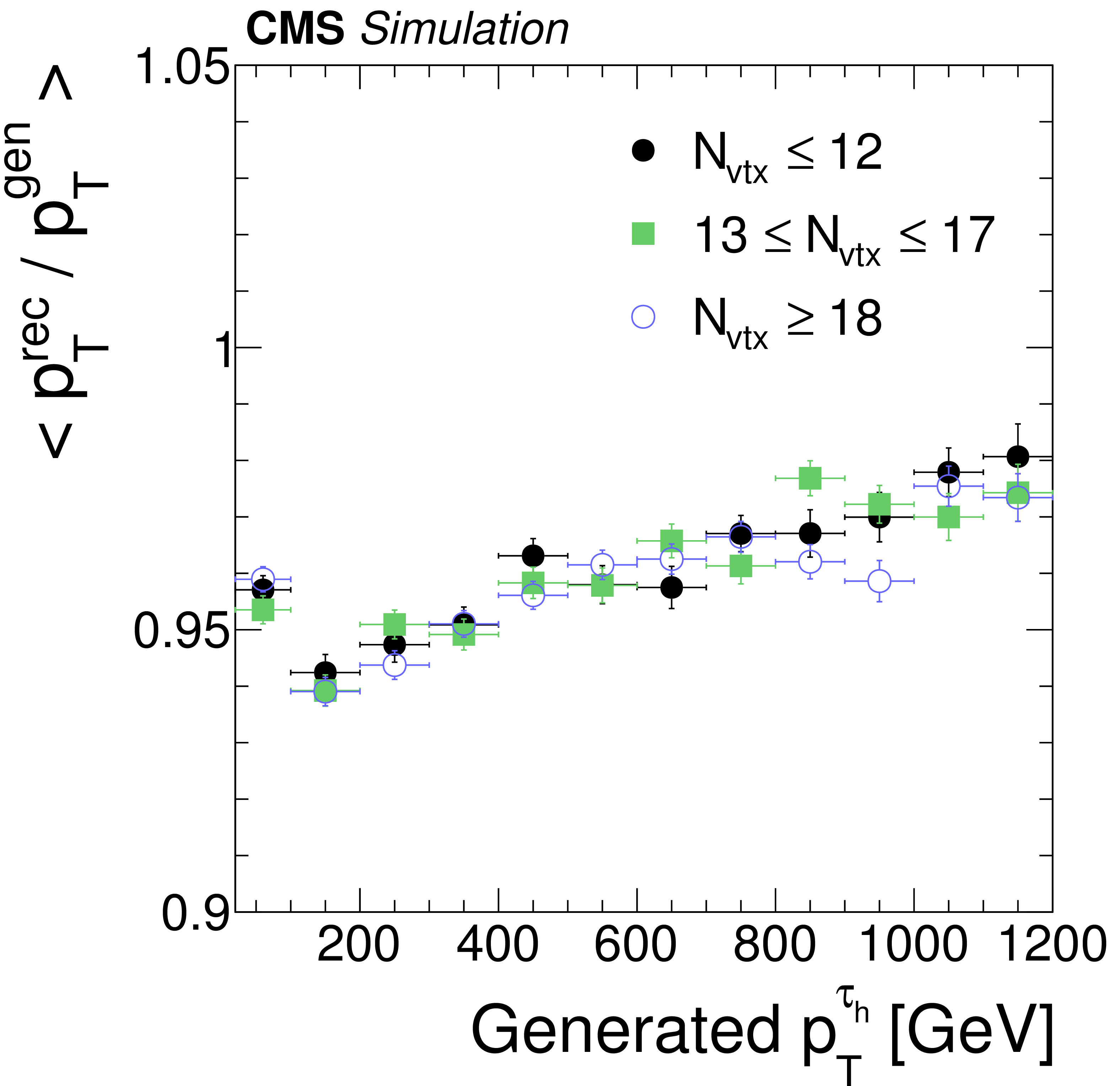
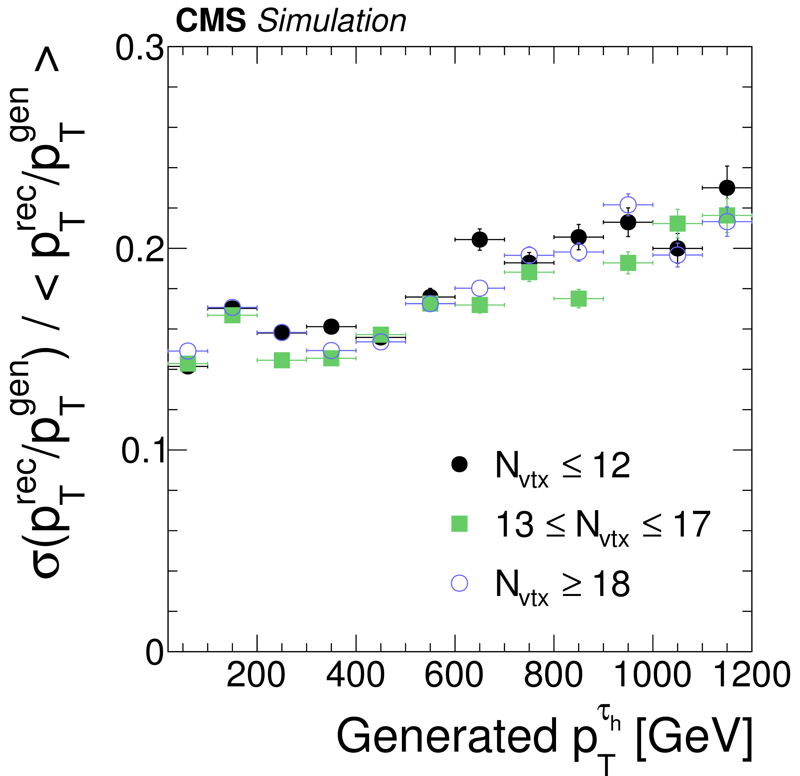
The $ { {\tau }_{\mathrm {h}}} $ energy response (a) and relative resolution (b) as function of generator-level visible $ {\tau }$ $ {p_{\mathrm {T}}} $ in simulated $ { {\mathrm {Z}}'} \to {\tau } {\tau }$ events for different pileup conditions: $ {N_{\text {vtx}}} \leq 12$, $13 \leq {N_{\text {vtx}}} \leq 17$, and $ {N_{\text {vtx}}} \geq 18$. Reconstructed $ { {\tau }_{\mathrm {h}}} $ candidates are required to be matched to hadronic $ {\tau }$ decays at the generator-level within $\Delta R < 0.3$, to be reconstructed in one of the decay modes $ {\mathrm {h}^{\pm }} $, $ {\mathrm {h}^{\pm } { {\pi ^0}}} $, $ {\mathrm {h}^{\pm } { {\pi ^0}} { {\pi ^0}}} $ or $ {\mathrm {h}^{\pm }\mathrm {h}^{\mp }\mathrm {h}^{\pm }} $, and to pass $ {p_{\mathrm {T}}} >$ 20 GeV, $ {| \eta | } <$ 2.3, and the loose WP of the cutoff-based $ { {\tau }_{\mathrm {h}}} $ isolation discriminant. |
png pdf |
Figure 8-b:
The $ { {\tau }_{\mathrm {h}}} $ energy response (a) and relative resolution (b) as function of generator-level visible $ {\tau }$ $ {p_{\mathrm {T}}} $ in simulated $ { {\mathrm {Z}}'} \to {\tau } {\tau }$ events for different pileup conditions: $ {N_{\text {vtx}}} \leq 12$, $13 \leq {N_{\text {vtx}}} \leq 17$, and $ {N_{\text {vtx}}} \geq 18$. Reconstructed $ { {\tau }_{\mathrm {h}}} $ candidates are required to be matched to hadronic $ {\tau }$ decays at the generator-level within $\Delta R < 0.3$, to be reconstructed in one of the decay modes $ {\mathrm {h}^{\pm }} $, $ {\mathrm {h}^{\pm } { {\pi ^0}}} $, $ {\mathrm {h}^{\pm } { {\pi ^0}} { {\pi ^0}}} $ or $ {\mathrm {h}^{\pm }\mathrm {h}^{\mp }\mathrm {h}^{\pm }} $, and to pass $ {p_{\mathrm {T}}} >$ 20 GeV, $ {| \eta | } <$ 2.3, and the loose WP of the cutoff-based $ { {\tau }_{\mathrm {h}}} $ isolation discriminant. |
png pdf |
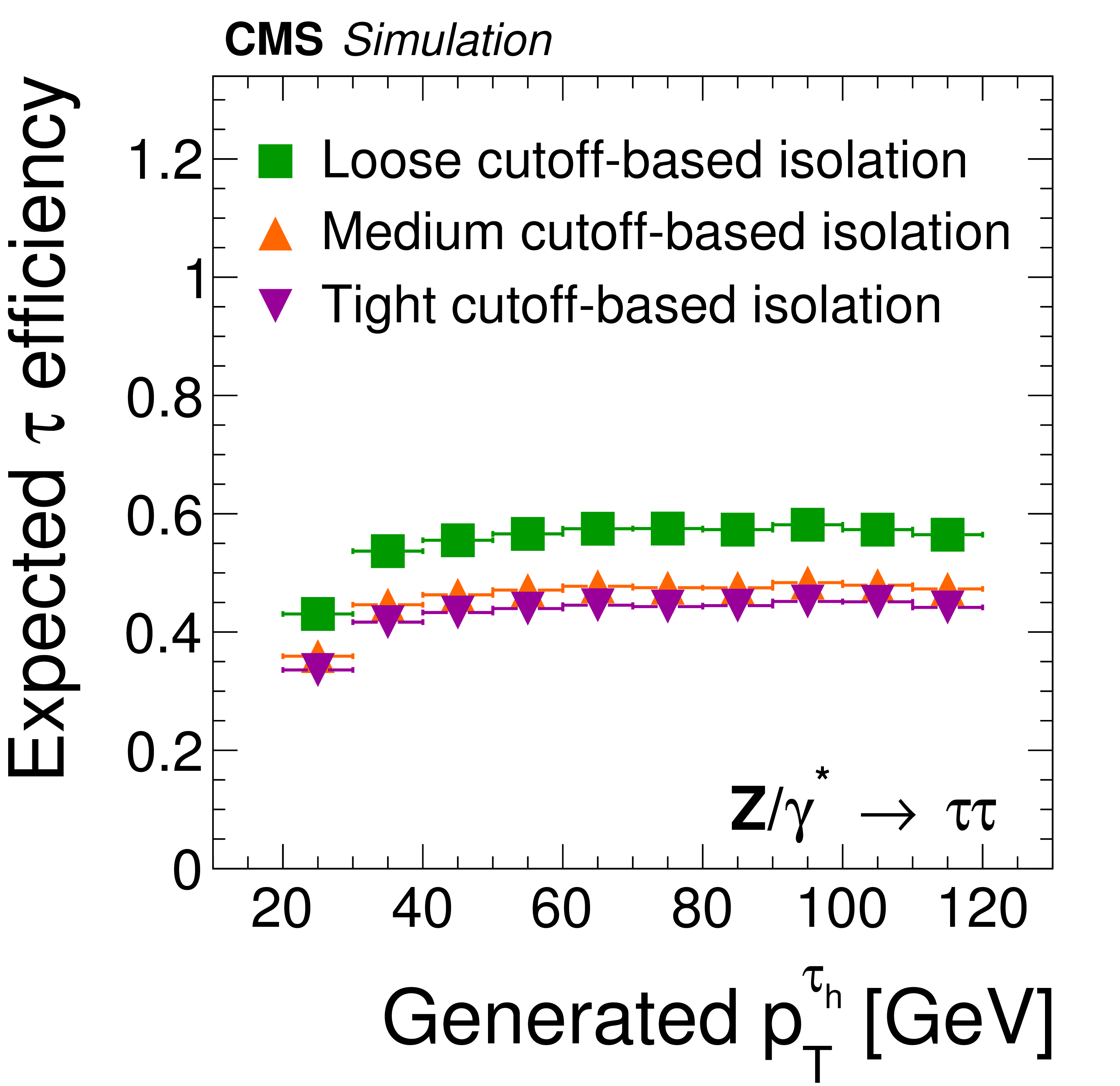
Figure 9-a:
Efficiency for $ { {\tau }_{\mathrm {h}}} $ decays in simulated $ {\mathrm {Z}}/ { {\gamma } ^{*}} \to {\tau } {\tau }$ (a,c) and $ { {\mathrm {Z}}'} \to {\tau } {\tau }$ (b,d) events to be reconstructed in one of the decay modes $ {\mathrm {h}^{\pm }} $, $ {\mathrm {h}^{\pm } { {\pi ^0}}} $, $ {\mathrm {h}^{\pm } { {\pi ^0}} { {\pi ^0}}} $, or $ {\mathrm {h}^{\pm }\mathrm {h}^{\mp }\mathrm {h}^{\pm }} $, to satisfy the conditions $ {p_{\mathrm {T}}} >$ 20 GeV and $ {| \eta | } <$ 2.3, and to pass: the loose, medium and tight WP of the cutoff-based $ { {\tau }_{\mathrm {h}}} $ isolation discriminant (a,b) and the very loose, loose, medium and tight WP of the MVA-based tau isolation discriminant (c,d). The efficiency is shown as a function of the generator-level $ {p_{\mathrm {T}}} $ of the visible $ {\tau }$ decay products in $ { {\tau }_{\mathrm {h}}} $ decays that are within $ {| \eta | } <$ 2.3. |
png pdf |
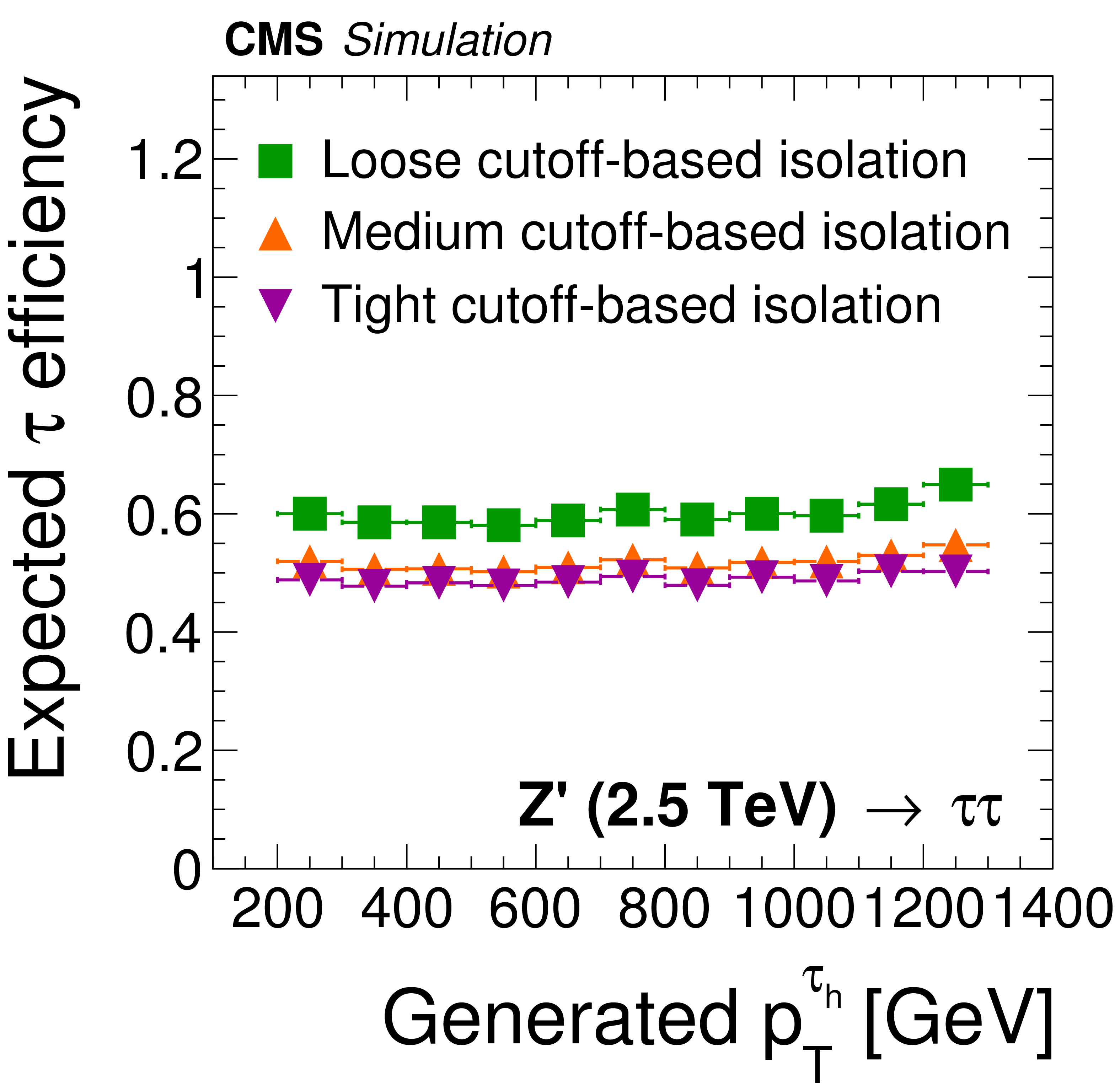
Figure 9-b:
Efficiency for $ { {\tau }_{\mathrm {h}}} $ decays in simulated $ {\mathrm {Z}}/ { {\gamma } ^{*}} \to {\tau } {\tau }$ (a,c) and $ { {\mathrm {Z}}'} \to {\tau } {\tau }$ (b,d) events to be reconstructed in one of the decay modes $ {\mathrm {h}^{\pm }} $, $ {\mathrm {h}^{\pm } { {\pi ^0}}} $, $ {\mathrm {h}^{\pm } { {\pi ^0}} { {\pi ^0}}} $, or $ {\mathrm {h}^{\pm }\mathrm {h}^{\mp }\mathrm {h}^{\pm }} $, to satisfy the conditions $ {p_{\mathrm {T}}} >$ 20 GeV and $ {| \eta | } <$ 2.3, and to pass: the loose, medium and tight WP of the cutoff-based $ { {\tau }_{\mathrm {h}}} $ isolation discriminant (a,b) and the very loose, loose, medium and tight WP of the MVA-based tau isolation discriminant (c,d). The efficiency is shown as a function of the generator-level $ {p_{\mathrm {T}}} $ of the visible $ {\tau }$ decay products in $ { {\tau }_{\mathrm {h}}} $ decays that are within $ {| \eta | } <$ 2.3. |
png pdf |
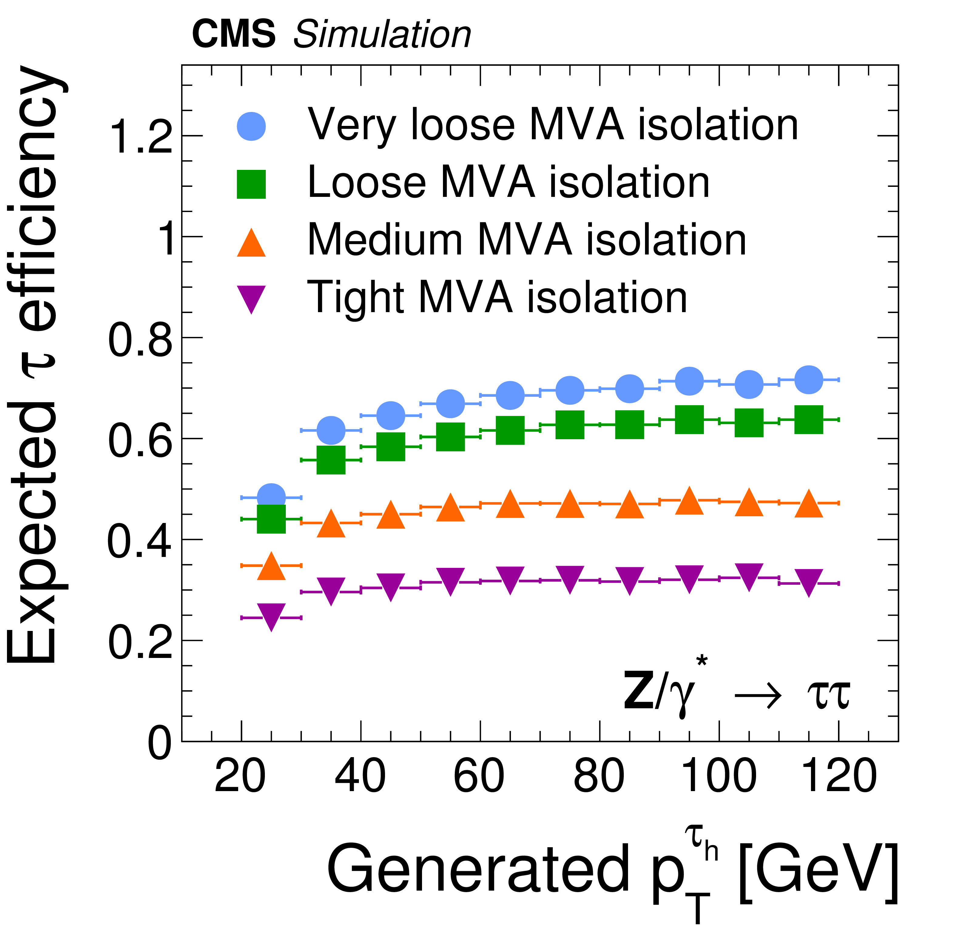
Figure 9-c:
Efficiency for $ { {\tau }_{\mathrm {h}}} $ decays in simulated $ {\mathrm {Z}}/ { {\gamma } ^{*}} \to {\tau } {\tau }$ (a,c) and $ { {\mathrm {Z}}'} \to {\tau } {\tau }$ (b,d) events to be reconstructed in one of the decay modes $ {\mathrm {h}^{\pm }} $, $ {\mathrm {h}^{\pm } { {\pi ^0}}} $, $ {\mathrm {h}^{\pm } { {\pi ^0}} { {\pi ^0}}} $, or $ {\mathrm {h}^{\pm }\mathrm {h}^{\mp }\mathrm {h}^{\pm }} $, to satisfy the conditions $ {p_{\mathrm {T}}} >$ 20 GeV and $ {| \eta | } <$ 2.3, and to pass: the loose, medium and tight WP of the cutoff-based $ { {\tau }_{\mathrm {h}}} $ isolation discriminant (a,b) and the very loose, loose, medium and tight WP of the MVA-based tau isolation discriminant (c,d). The efficiency is shown as a function of the generator-level $ {p_{\mathrm {T}}} $ of the visible $ {\tau }$ decay products in $ { {\tau }_{\mathrm {h}}} $ decays that are within $ {| \eta | } <$ 2.3. |
png pdf |
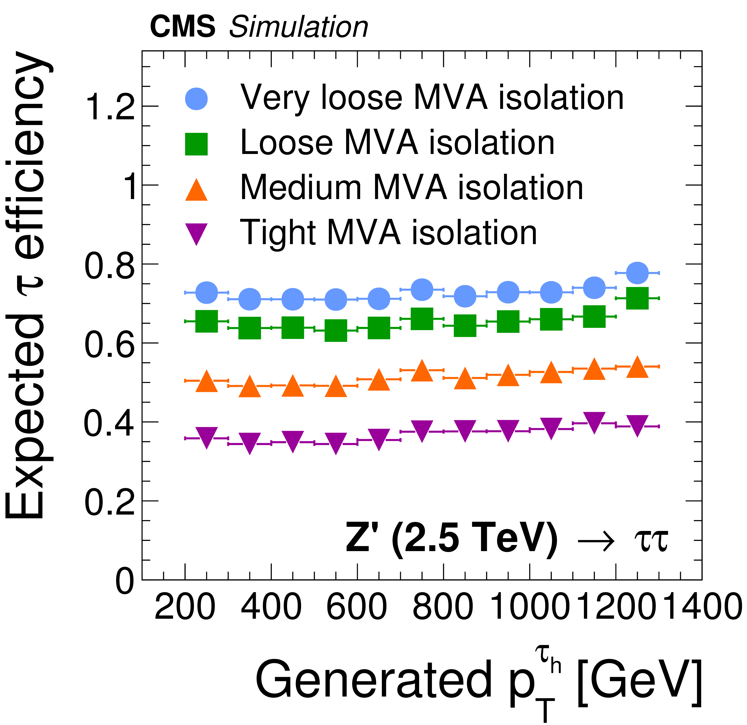
Figure 9-d:
Efficiency for $ { {\tau }_{\mathrm {h}}} $ decays in simulated $ {\mathrm {Z}}/ { {\gamma } ^{*}} \to {\tau } {\tau }$ (a,c) and $ { {\mathrm {Z}}'} \to {\tau } {\tau }$ (b,d) events to be reconstructed in one of the decay modes $ {\mathrm {h}^{\pm }} $, $ {\mathrm {h}^{\pm } { {\pi ^0}}} $, $ {\mathrm {h}^{\pm } { {\pi ^0}} { {\pi ^0}}} $, or $ {\mathrm {h}^{\pm }\mathrm {h}^{\mp }\mathrm {h}^{\pm }} $, to satisfy the conditions $ {p_{\mathrm {T}}} >$ 20 GeV and $ {| \eta | } <$ 2.3, and to pass: the loose, medium and tight WP of the cutoff-based $ { {\tau }_{\mathrm {h}}} $ isolation discriminant (a,b) and the very loose, loose, medium and tight WP of the MVA-based tau isolation discriminant (c,d). The efficiency is shown as a function of the generator-level $ {p_{\mathrm {T}}} $ of the visible $ {\tau }$ decay products in $ { {\tau }_{\mathrm {h}}} $ decays that are within $ {| \eta | } <$ 2.3. |
png pdf |
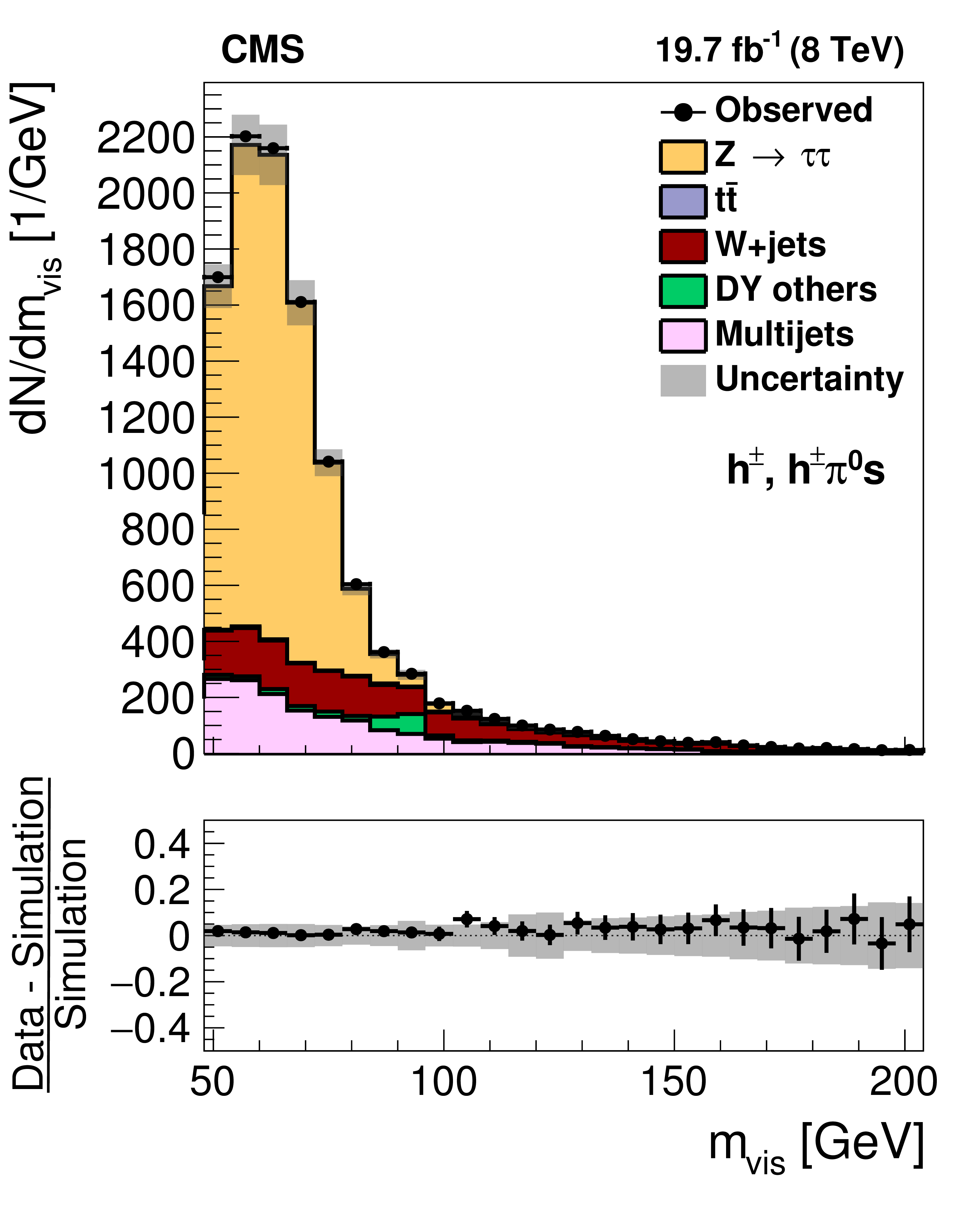
Figure 10-a:
a,b: Distribution in the visible mass of $ {\mathrm {Z}}/ { {\gamma } ^{*}} \to {\tau } {\tau }\to {{\mu }} { {\tau }_{\mathrm {h}}} $ candidate events, in which the reconstructed $ { {\tau }_{\mathrm {h}}} $ candidate contains (a) a single or (b) three charged particles. c,d: Distribution in (c) transverse impact parameter for events in which the $ { {\tau }_{\mathrm {h}}} $ candidate contains one charged particle and (d) in the distance between the $ {\tau }$ production and decay vertex for events in which the $ { {\tau }_{\mathrm {h}}} $ candidate contains three charged particles. The $ {\mathrm {Z}}/ { {\gamma } ^{*}} \to {\ell } {\ell }$ ($ {\ell }= {\mathrm {e}}$, $ {{\mu }}$, $ {\tau }$) events in which either the reconstructed muon or the reconstructed $ { {\tau }_{\mathrm {h}}} $ candidate are misidentified are denoted by ``DY others''. |
png pdf |
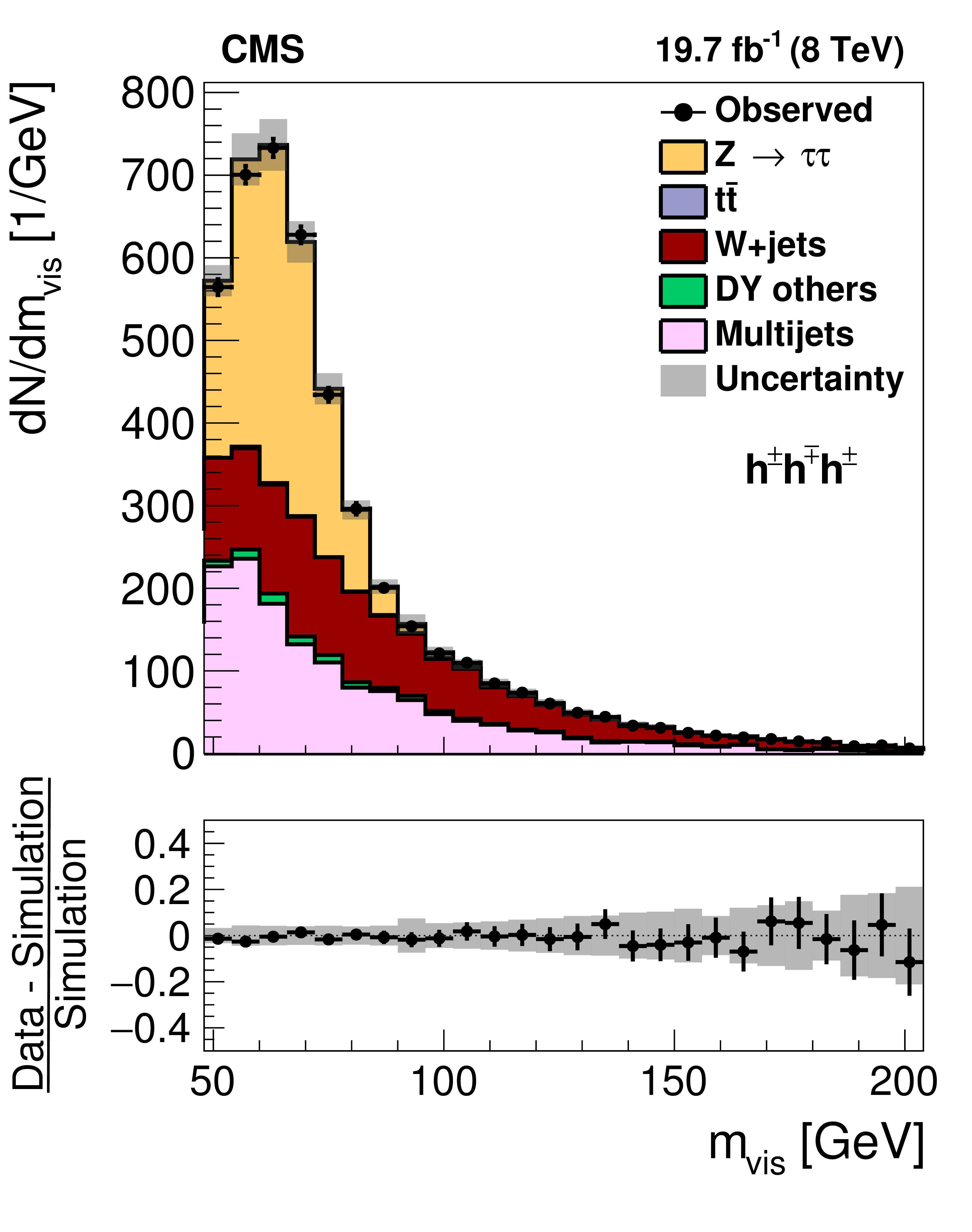
Figure 10-b:
a,b: Distribution in the visible mass of $ {\mathrm {Z}}/ { {\gamma } ^{*}} \to {\tau } {\tau }\to {{\mu }} { {\tau }_{\mathrm {h}}} $ candidate events, in which the reconstructed $ { {\tau }_{\mathrm {h}}} $ candidate contains (a) a single or (b) three charged particles. c,d: Distribution in (c) transverse impact parameter for events in which the $ { {\tau }_{\mathrm {h}}} $ candidate contains one charged particle and (d) in the distance between the $ {\tau }$ production and decay vertex for events in which the $ { {\tau }_{\mathrm {h}}} $ candidate contains three charged particles. The $ {\mathrm {Z}}/ { {\gamma } ^{*}} \to {\ell } {\ell }$ ($ {\ell }= {\mathrm {e}}$, $ {{\mu }}$, $ {\tau }$) events in which either the reconstructed muon or the reconstructed $ { {\tau }_{\mathrm {h}}} $ candidate are misidentified are denoted by ``DY others''. |
png pdf |
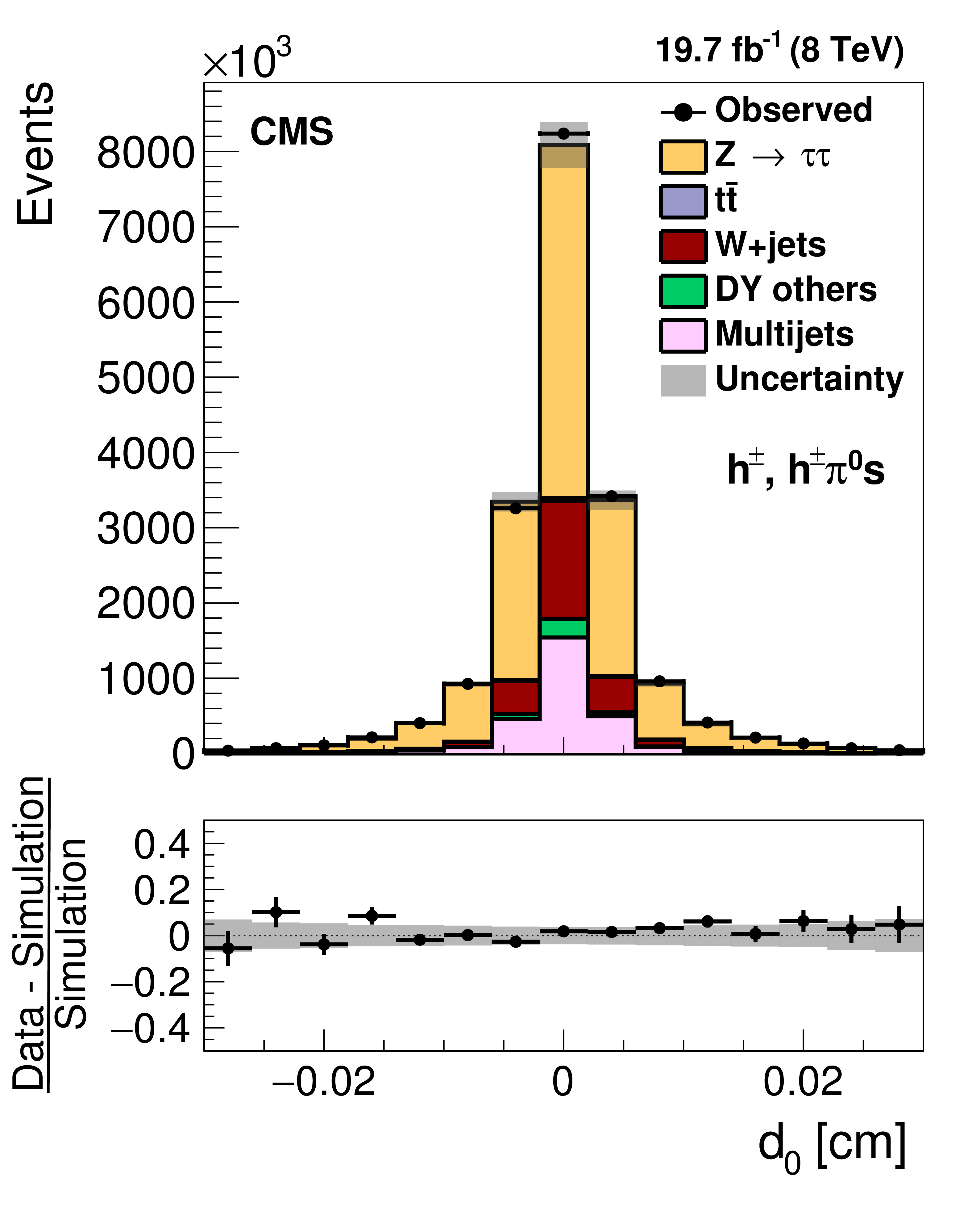
Figure 10-c:
a,b: Distribution in the visible mass of $ {\mathrm {Z}}/ { {\gamma } ^{*}} \to {\tau } {\tau }\to {{\mu }} { {\tau }_{\mathrm {h}}} $ candidate events, in which the reconstructed $ { {\tau }_{\mathrm {h}}} $ candidate contains (a) a single or (b) three charged particles. c,d: Distribution in (c) transverse impact parameter for events in which the $ { {\tau }_{\mathrm {h}}} $ candidate contains one charged particle and (d) in the distance between the $ {\tau }$ production and decay vertex for events in which the $ { {\tau }_{\mathrm {h}}} $ candidate contains three charged particles. The $ {\mathrm {Z}}/ { {\gamma } ^{*}} \to {\ell } {\ell }$ ($ {\ell }= {\mathrm {e}}$, $ {{\mu }}$, $ {\tau }$) events in which either the reconstructed muon or the reconstructed $ { {\tau }_{\mathrm {h}}} $ candidate are misidentified are denoted by ``DY others''. |
png pdf |
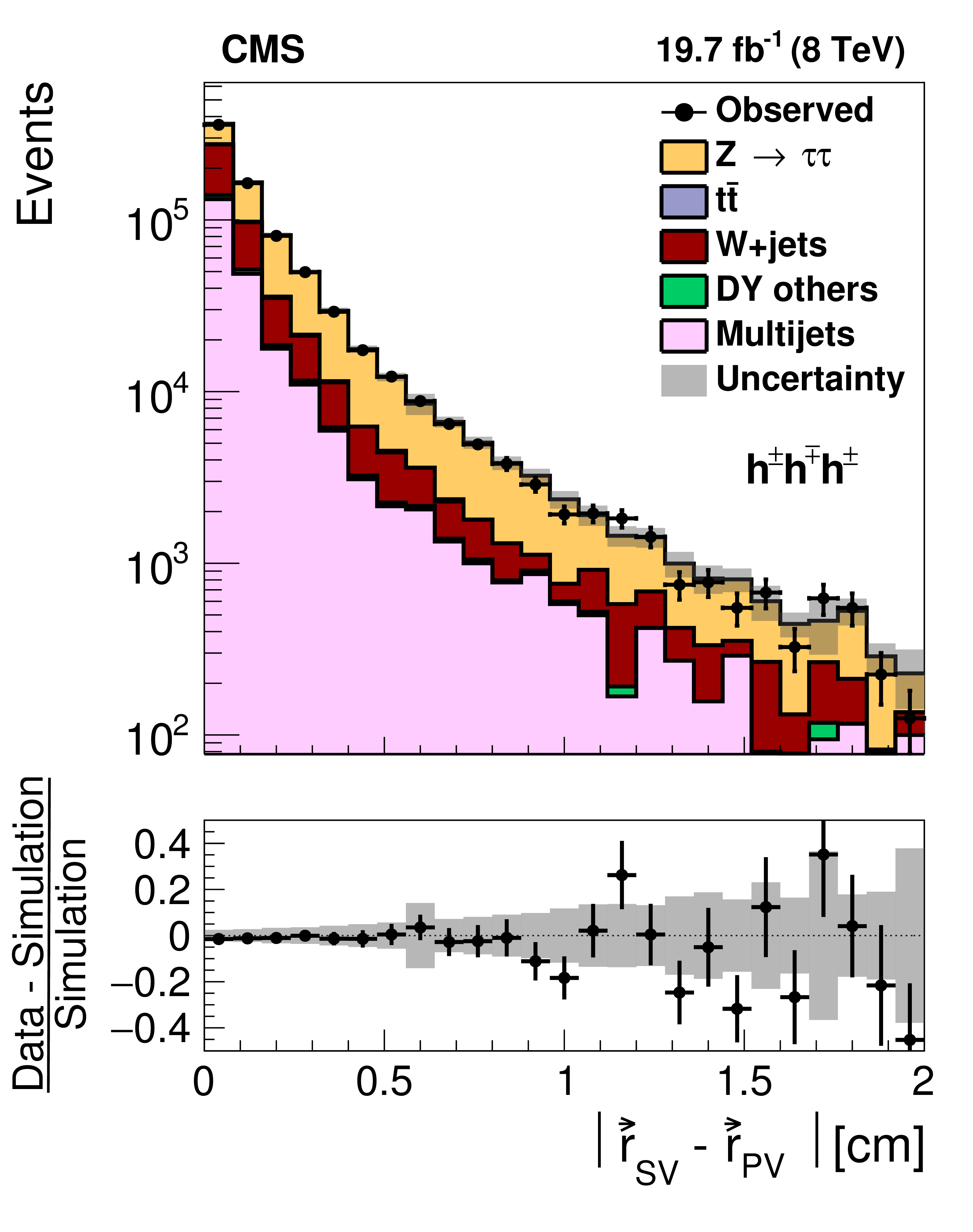
Figure 10-d:
a,b: Distribution in the visible mass of $ {\mathrm {Z}}/ { {\gamma } ^{*}} \to {\tau } {\tau }\to {{\mu }} { {\tau }_{\mathrm {h}}} $ candidate events, in which the reconstructed $ { {\tau }_{\mathrm {h}}} $ candidate contains (a) a single or (b) three charged particles. c,d: Distribution in (c) transverse impact parameter for events in which the $ { {\tau }_{\mathrm {h}}} $ candidate contains one charged particle and (d) in the distance between the $ {\tau }$ production and decay vertex for events in which the $ { {\tau }_{\mathrm {h}}} $ candidate contains three charged particles. The $ {\mathrm {Z}}/ { {\gamma } ^{*}} \to {\ell } {\ell }$ ($ {\ell }= {\mathrm {e}}$, $ {{\mu }}$, $ {\tau }$) events in which either the reconstructed muon or the reconstructed $ { {\tau }_{\mathrm {h}}} $ candidate are misidentified are denoted by ``DY others''. |
png pdf |
Figure 11-a:
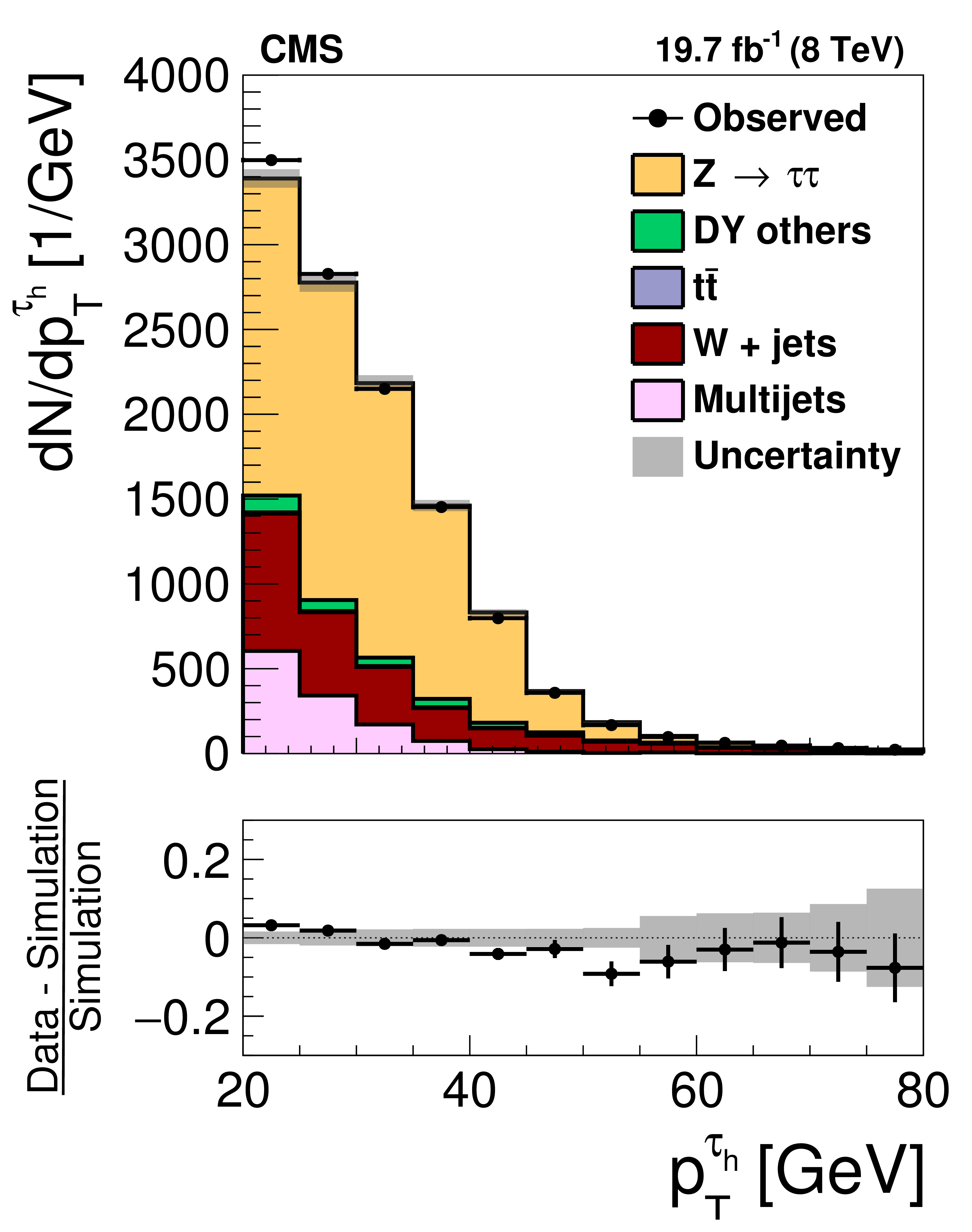
Distribution in the $ {p_{\mathrm {T}}} $ of $ { {\tau }_{\mathrm {h}}} $ candidates in (a) $ {\mathrm {Z}}/ { {\gamma } ^{*}} \to {\tau } {\tau }$ and (b) $ {\mathrm {t}} {\overline {\mathrm {t}}}$ events in data and in simulations. The $ {\mathrm {Z}}/ { {\gamma } ^{*}} \to {\ell } {\ell }$ ($ {\ell }= {\mathrm {e}}$, $ {{\mu }}$, $ {\tau }$) and $ {\mathrm {t}} {\overline {\mathrm {t}}}$ events in which either the reconstructed muon or the reconstructed $ { {\tau }_{\mathrm {h}}} $ candidate is misidentified are denoted in the MC simulation by ``DY others'' and ``$ {\mathrm {t}} {\overline {\mathrm {t}}}$ others'', respectively. |
png pdf |
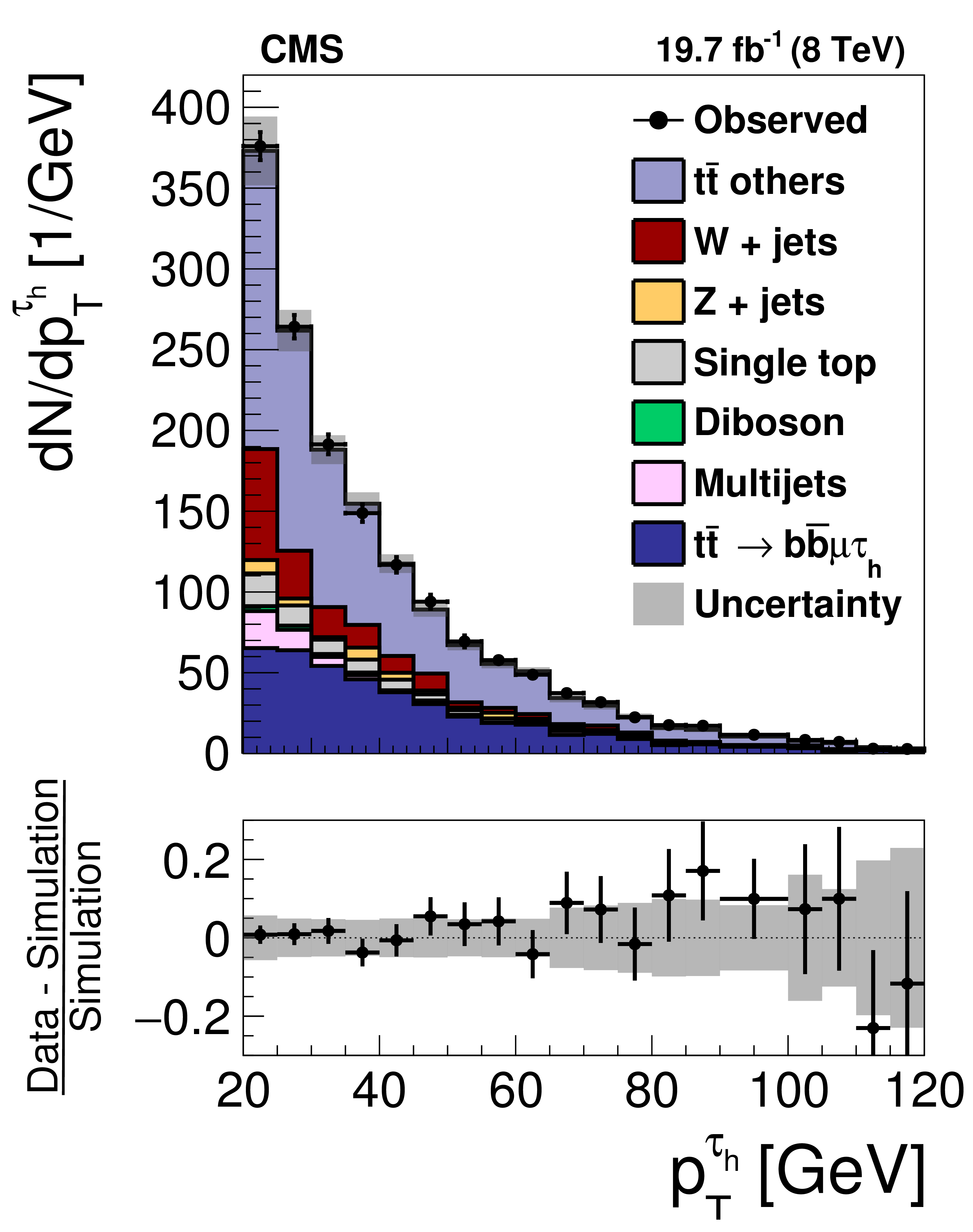
Figure 11-b:
Distribution in the $ {p_{\mathrm {T}}} $ of $ { {\tau }_{\mathrm {h}}} $ candidates in (a) $ {\mathrm {Z}}/ { {\gamma } ^{*}} \to {\tau } {\tau }$ and (b) $ {\mathrm {t}} {\overline {\mathrm {t}}}$ events in data and in simulations. The $ {\mathrm {Z}}/ { {\gamma } ^{*}} \to {\ell } {\ell }$ ($ {\ell }= {\mathrm {e}}$, $ {{\mu }}$, $ {\tau }$) and $ {\mathrm {t}} {\overline {\mathrm {t}}}$ events in which either the reconstructed muon or the reconstructed $ { {\tau }_{\mathrm {h}}} $ candidate is misidentified are denoted in the MC simulation by ``DY others'' and ``$ {\mathrm {t}} {\overline {\mathrm {t}}}$ others'', respectively. |
png pdf |
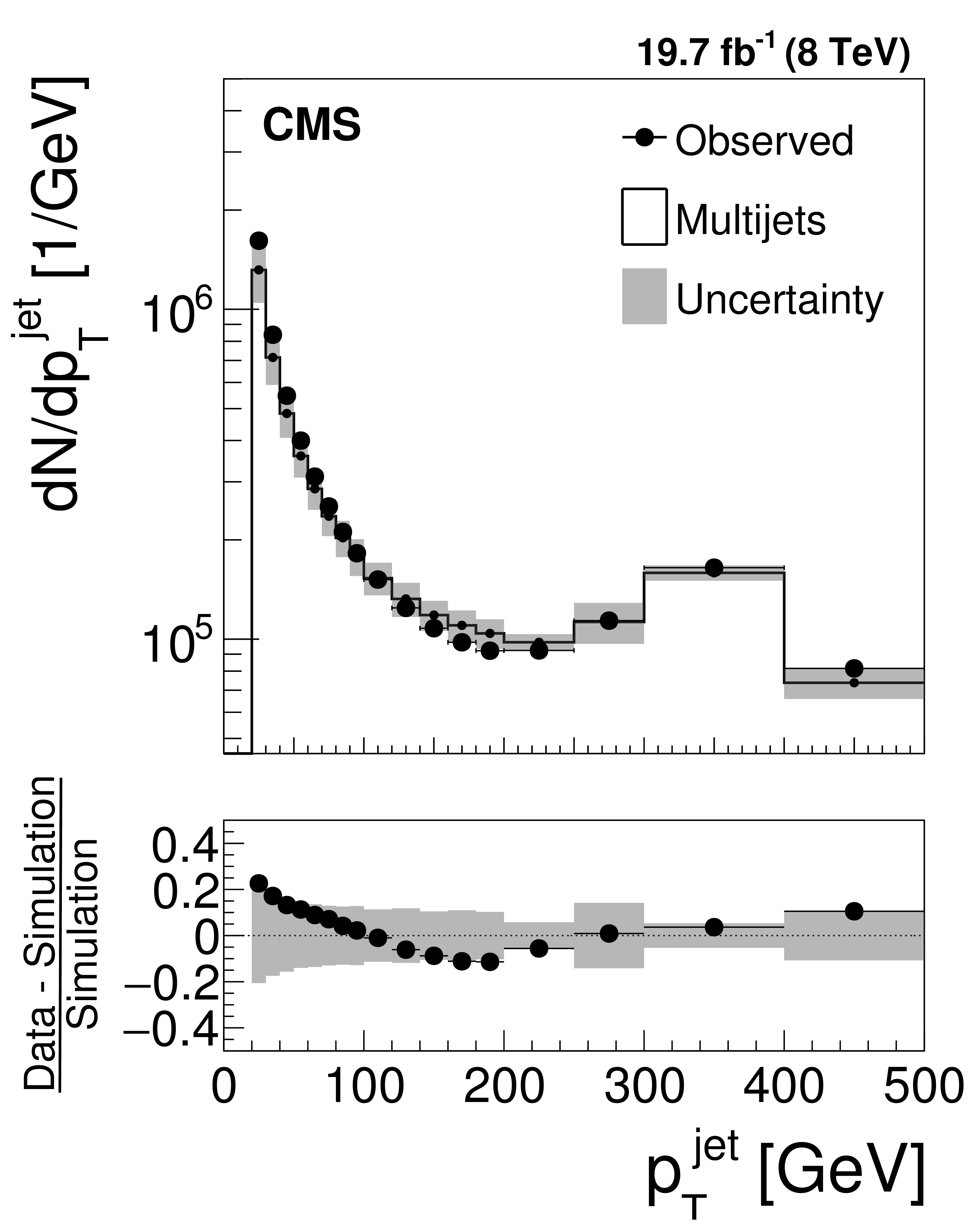
Figure 12-a:
Jet $ {p_{\mathrm {T}}} $ distribution in (a) multijet and (b) W+jets events observed in data, compared to the MC expectation. The uncertainty in the MC expectation is dominated by the uncertainty in the jet energy scale. |

png pdf |
Figure 12-b:
Jet $ {p_{\mathrm {T}}} $ distribution in (a) multijet and (b) W+jets events observed in data, compared to the MC expectation. The uncertainty in the MC expectation is dominated by the uncertainty in the jet energy scale. |
png pdf |
Figure 13-a:
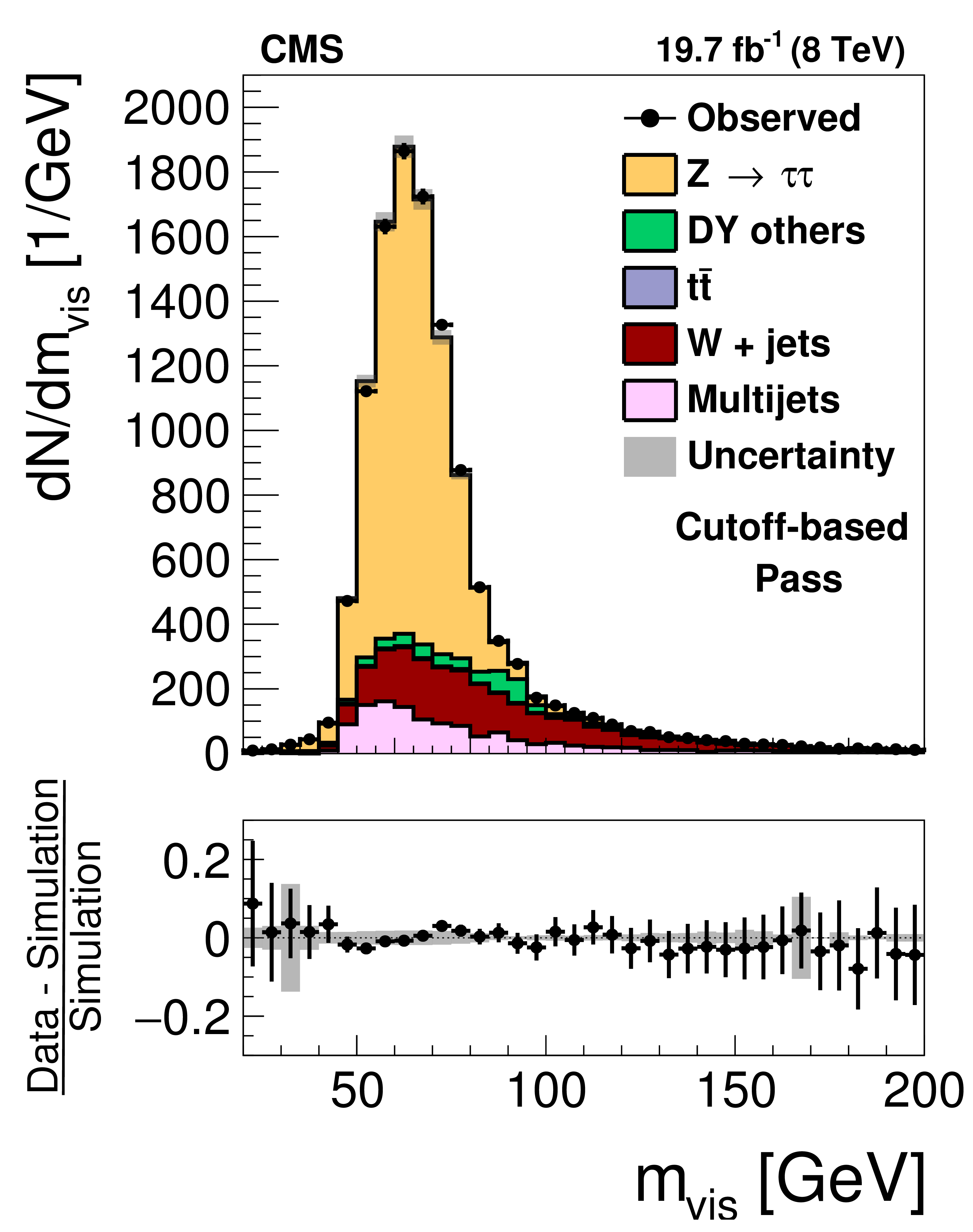
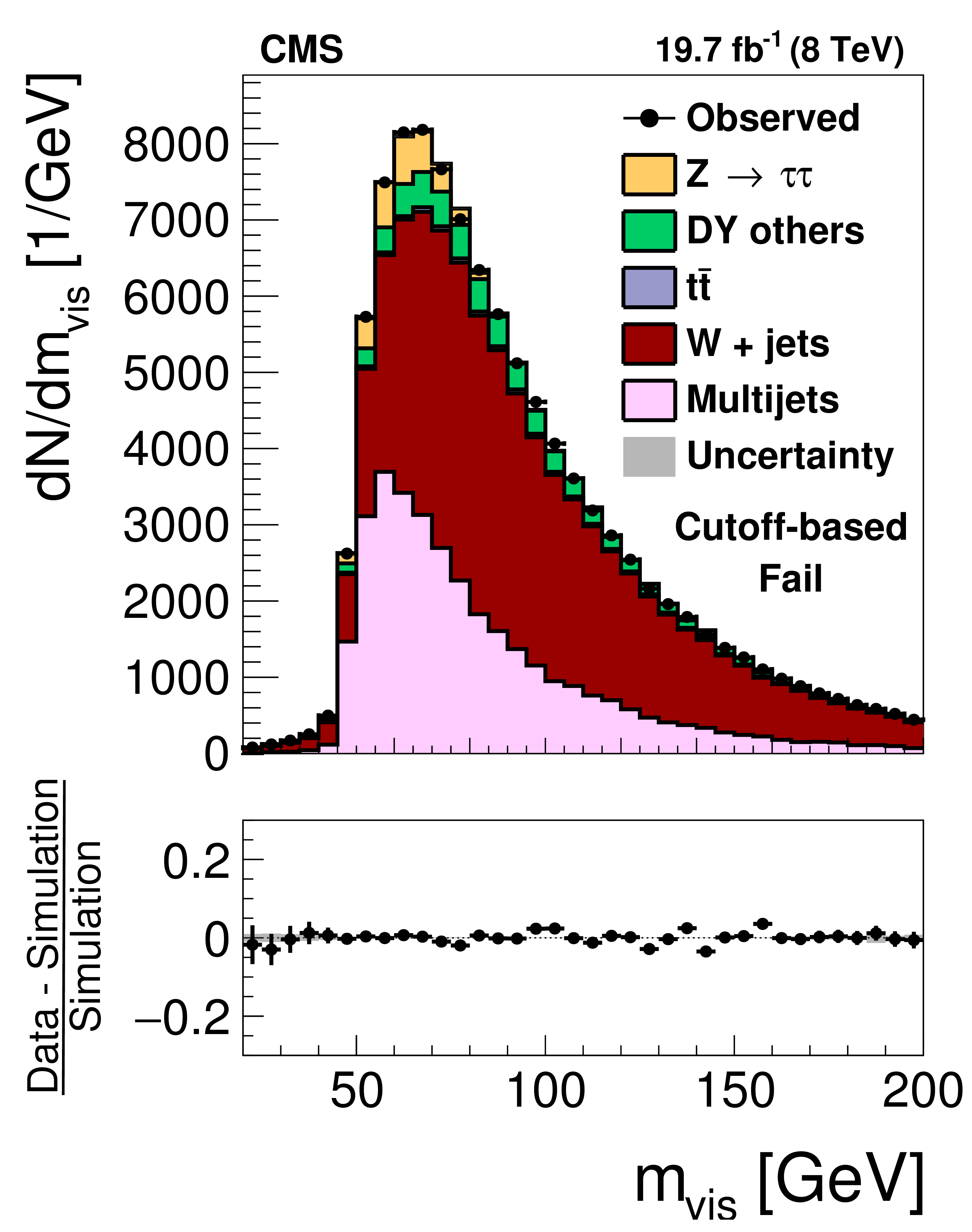
Distribution in $ {m_{\text {vis}}} $ observed in the pass (a,c) and fail (b,d) samples of $ {\mathrm {Z}}/ { {\gamma } ^{*}} \to {\tau } {\tau }$ candidate events used to measure the $ { {\tau }_{\mathrm {h}}} $ identification efficiency, compared to the MC expectation, for the loose WP of the cutoff-based (a,b) and MVA-based (c,d) $ { {\tau }_{\mathrm {h}}} $ isolation discriminants. $ {\mathrm {Z}}/ { {\gamma } ^{*}} \to {\ell } {\ell }$ ($ {\ell }= {\mathrm {e}}$, $ {{\mu }}$, $ {\tau }$) events in which either the reconstructed muon or the reconstructed $ { {\tau }_{\mathrm {h}}} $ candidate is due to a misidentification are denoted by ``DY others''. The expected $ {m_{\text {vis}}} $ distribution is shown for the values of nuisance parameters obtained from the likelihood fit to the data, described in Section 7.3. The ``Uncertainty'' bands represent the statistical and systematic uncertainties added in quadrature. |
png pdf |
Figure 13-b:
Distribution in $ {m_{\text {vis}}} $ observed in the pass (a,c) and fail (b,d) samples of $ {\mathrm {Z}}/ { {\gamma } ^{*}} \to {\tau } {\tau }$ candidate events used to measure the $ { {\tau }_{\mathrm {h}}} $ identification efficiency, compared to the MC expectation, for the loose WP of the cutoff-based (a,b) and MVA-based (c,d) $ { {\tau }_{\mathrm {h}}} $ isolation discriminants. $ {\mathrm {Z}}/ { {\gamma } ^{*}} \to {\ell } {\ell }$ ($ {\ell }= {\mathrm {e}}$, $ {{\mu }}$, $ {\tau }$) events in which either the reconstructed muon or the reconstructed $ { {\tau }_{\mathrm {h}}} $ candidate is due to a misidentification are denoted by ``DY others''. The expected $ {m_{\text {vis}}} $ distribution is shown for the values of nuisance parameters obtained from the likelihood fit to the data, described in Section 7.3. The ``Uncertainty'' bands represent the statistical and systematic uncertainties added in quadrature. |

png pdf |
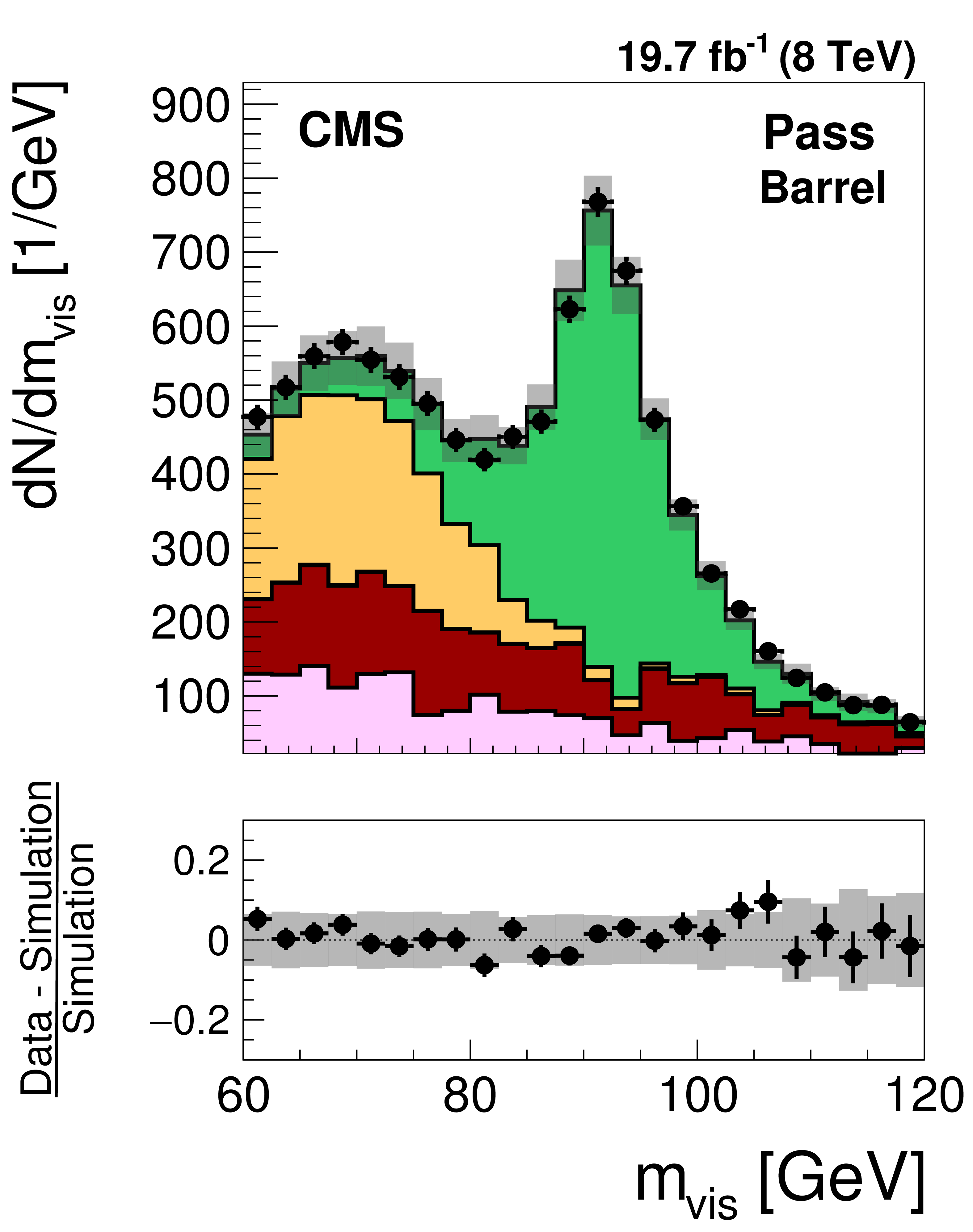
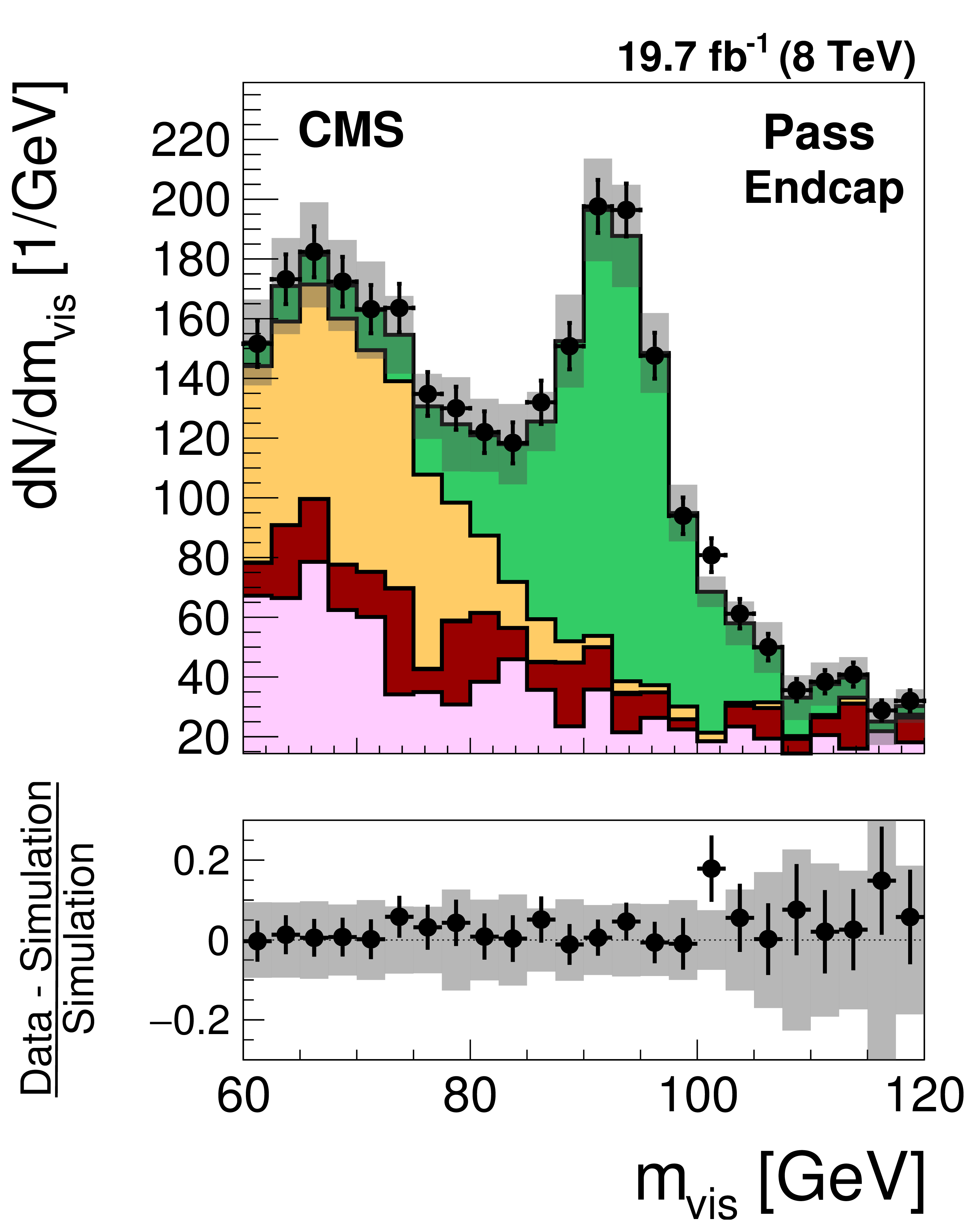
Figure 13-c:
Distribution in $ {m_{\text {vis}}} $ observed in the pass (a,c) and fail (b,d) samples of $ {\mathrm {Z}}/ { {\gamma } ^{*}} \to {\tau } {\tau }$ candidate events used to measure the $ { {\tau }_{\mathrm {h}}} $ identification efficiency, compared to the MC expectation, for the loose WP of the cutoff-based (a,b) and MVA-based (c,d) $ { {\tau }_{\mathrm {h}}} $ isolation discriminants. $ {\mathrm {Z}}/ { {\gamma } ^{*}} \to {\ell } {\ell }$ ($ {\ell }= {\mathrm {e}}$, $ {{\mu }}$, $ {\tau }$) events in which either the reconstructed muon or the reconstructed $ { {\tau }_{\mathrm {h}}} $ candidate is due to a misidentification are denoted by ``DY others''. The expected $ {m_{\text {vis}}} $ distribution is shown for the values of nuisance parameters obtained from the likelihood fit to the data, described in Section 7.3. The ``Uncertainty'' bands represent the statistical and systematic uncertainties added in quadrature. |

png pdf |
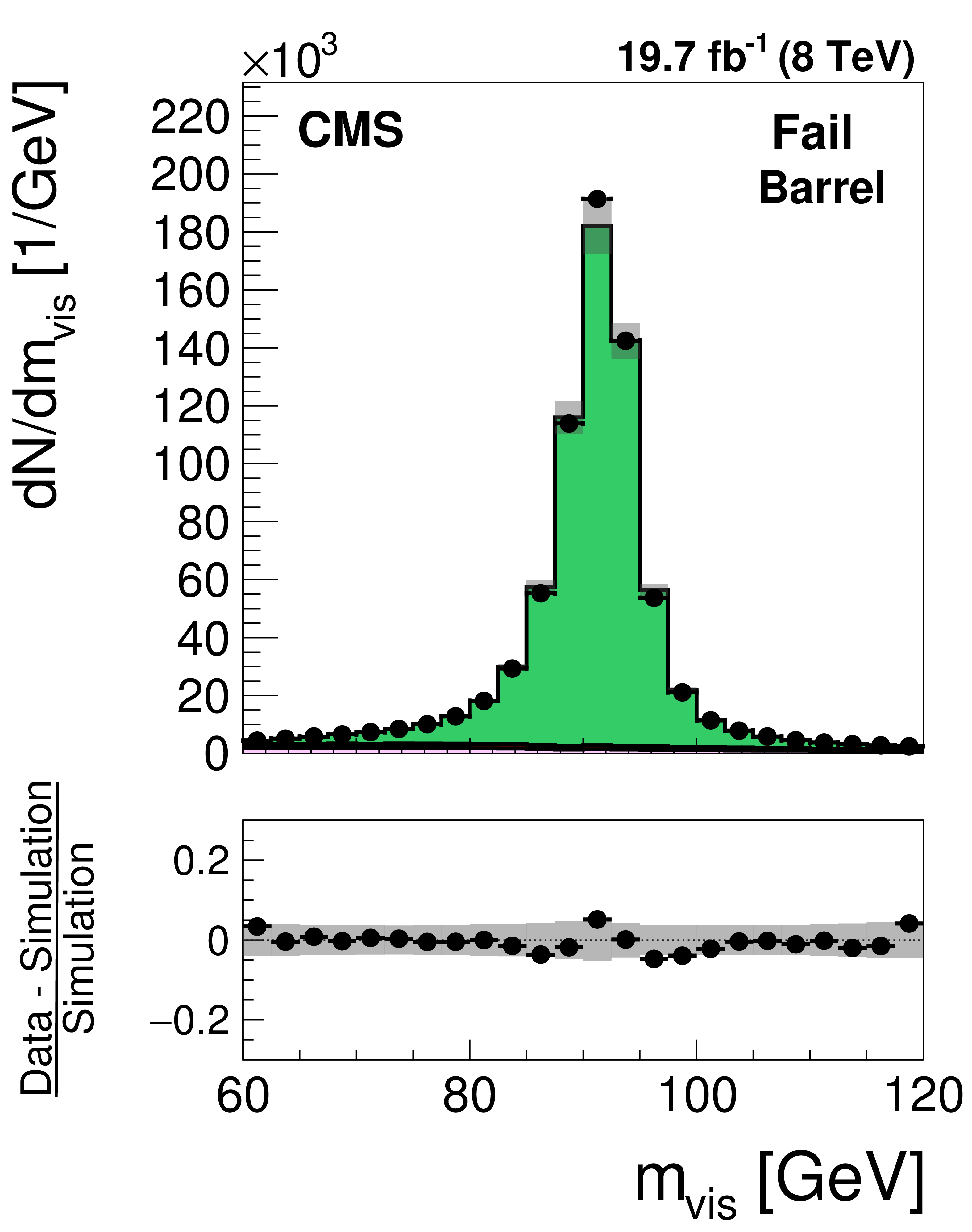
Figure 13-d:
Distribution in $ {m_{\text {vis}}} $ observed in the pass (a,c) and fail (b,d) samples of $ {\mathrm {Z}}/ { {\gamma } ^{*}} \to {\tau } {\tau }$ candidate events used to measure the $ { {\tau }_{\mathrm {h}}} $ identification efficiency, compared to the MC expectation, for the loose WP of the cutoff-based (a,b) and MVA-based (c,d) $ { {\tau }_{\mathrm {h}}} $ isolation discriminants. $ {\mathrm {Z}}/ { {\gamma } ^{*}} \to {\ell } {\ell }$ ($ {\ell }= {\mathrm {e}}$, $ {{\mu }}$, $ {\tau }$) events in which either the reconstructed muon or the reconstructed $ { {\tau }_{\mathrm {h}}} $ candidate is due to a misidentification are denoted by ``DY others''. The expected $ {m_{\text {vis}}} $ distribution is shown for the values of nuisance parameters obtained from the likelihood fit to the data, described in Section 7.3. The ``Uncertainty'' bands represent the statistical and systematic uncertainties added in quadrature. |

png pdf |
Figure 14-a:
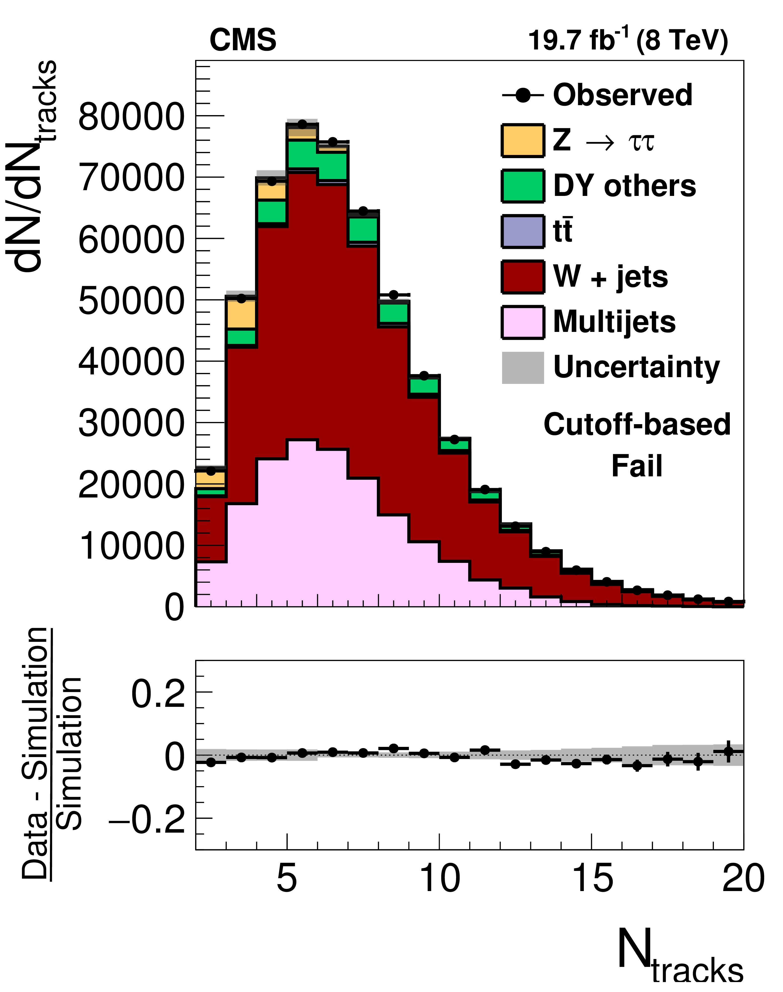
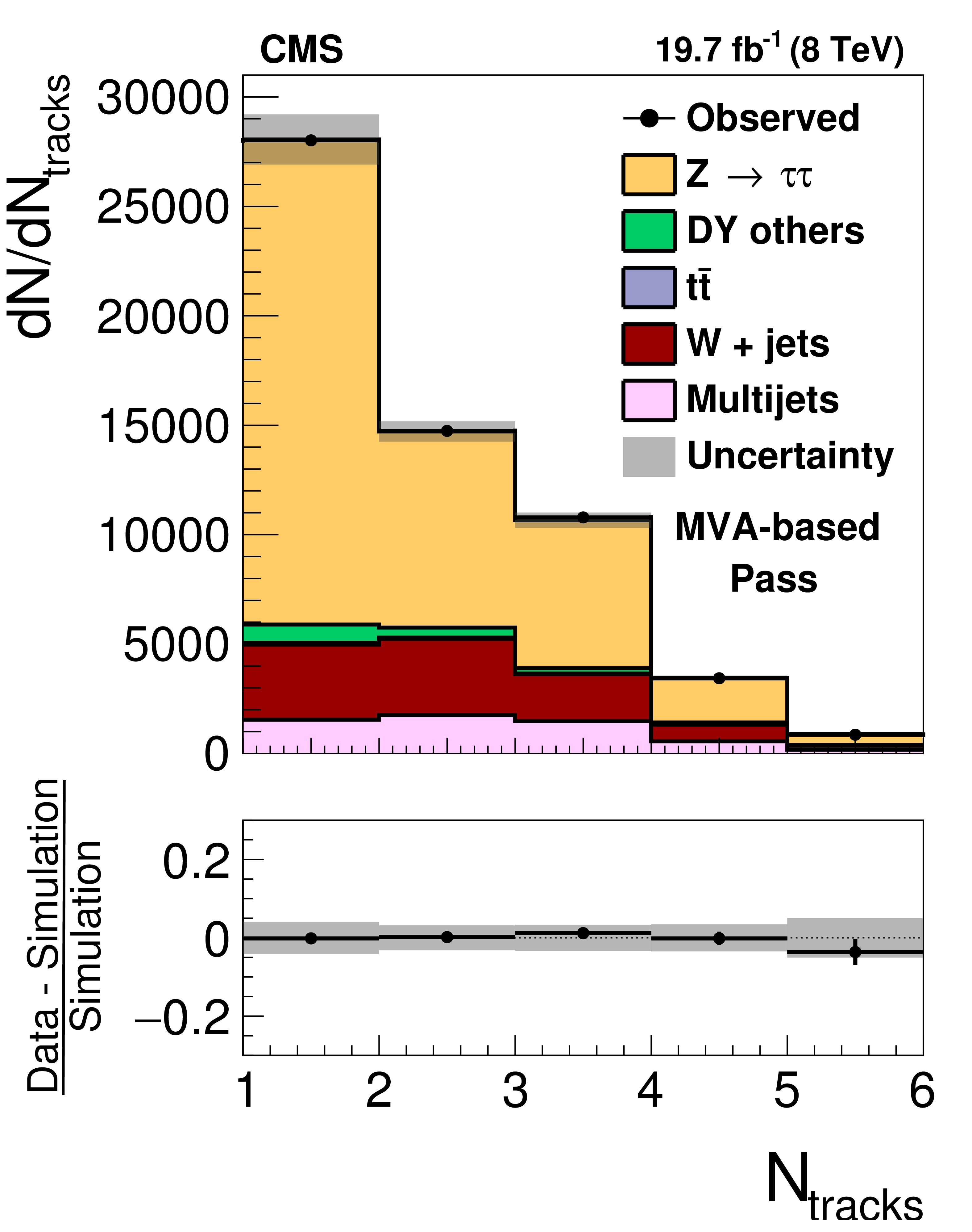
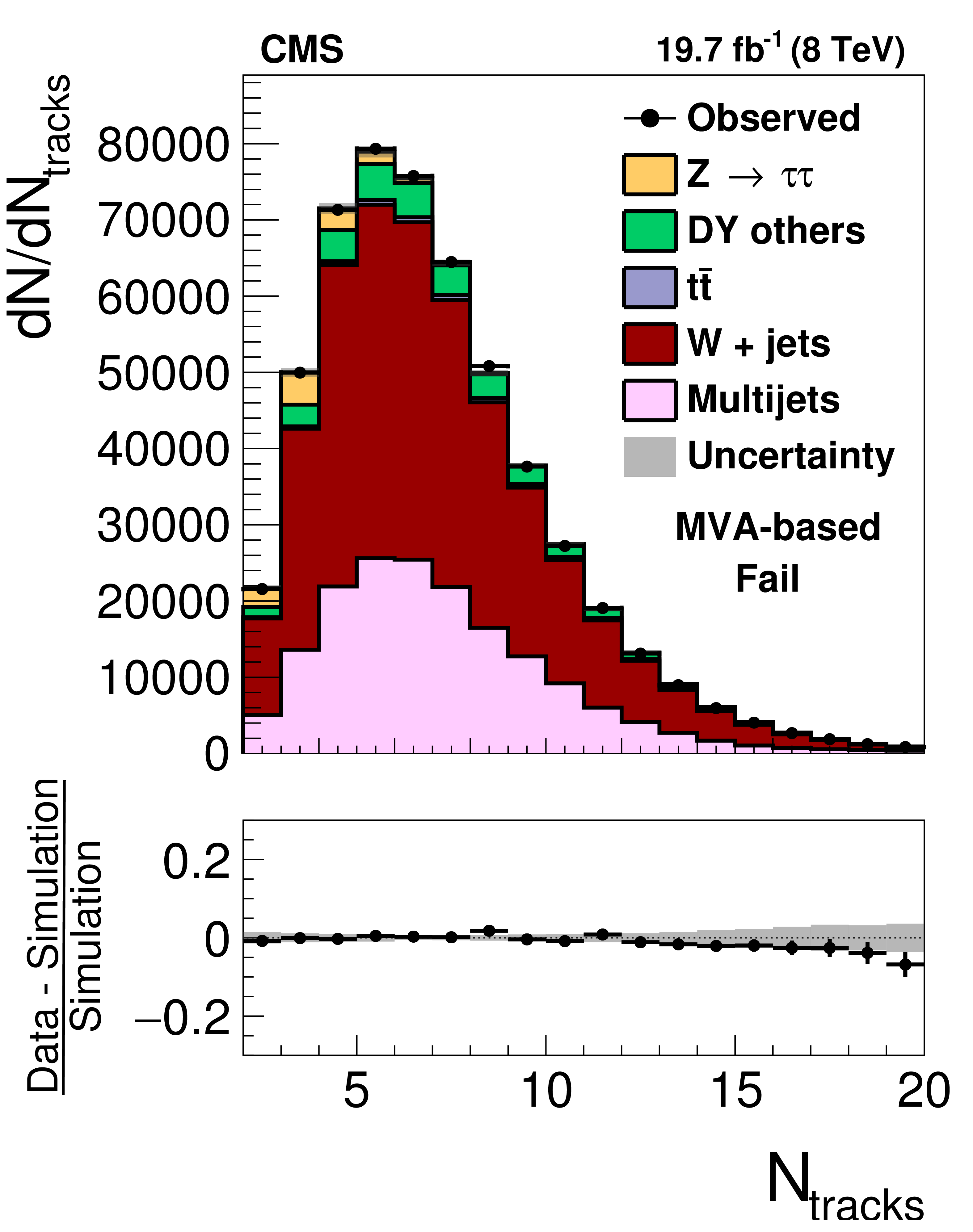
Distribution in $ {N_{\text {tracks}}} $ observed in the pass (a,c) and fail (b,d) samples of $ {\mathrm {Z}}/ { {\gamma } ^{*}} \to {\tau } {\tau }$ candidate events used to measure the $ { {\tau }_{\mathrm {h}}} $ identification efficiency, compared to the MC expectation, for the loose WP of the cutoff-based (a,b) and MVA-based (c,d) $ { {\tau }_{\mathrm {h}}} $ isolation discriminants. $ {\mathrm {Z}}/ { {\gamma } ^{*}} \to {\ell } {\ell }$ ($ {\ell }= {\mathrm {e}}$, $ {{\mu }}$, $ {\tau }$) events in which either the reconstructed muon or the reconstructed $ { {\tau }_{\mathrm {h}}} $ candidate is due to a misidentification are denoted by ``DY others''. The expected $ {N_{\text {tracks}}} $ distribution is shown for the values of nuisance parameters obtained from the likelihood fit to the data, described in Section 7.3. The ``Uncertainty'' bands represent the statistical and systematic uncertainties added in quadrature. |
png pdf |
Figure 14-b:
Distribution in $ {N_{\text {tracks}}} $ observed in the pass (a,c) and fail (b,d) samples of $ {\mathrm {Z}}/ { {\gamma } ^{*}} \to {\tau } {\tau }$ candidate events used to measure the $ { {\tau }_{\mathrm {h}}} $ identification efficiency, compared to the MC expectation, for the loose WP of the cutoff-based (a,b) and MVA-based (c,d) $ { {\tau }_{\mathrm {h}}} $ isolation discriminants. $ {\mathrm {Z}}/ { {\gamma } ^{*}} \to {\ell } {\ell }$ ($ {\ell }= {\mathrm {e}}$, $ {{\mu }}$, $ {\tau }$) events in which either the reconstructed muon or the reconstructed $ { {\tau }_{\mathrm {h}}} $ candidate is due to a misidentification are denoted by ``DY others''. The expected $ {N_{\text {tracks}}} $ distribution is shown for the values of nuisance parameters obtained from the likelihood fit to the data, described in Section 7.3. The ``Uncertainty'' bands represent the statistical and systematic uncertainties added in quadrature. |
png pdf |
Figure 14-c:
Distribution in $ {N_{\text {tracks}}} $ observed in the pass (a,c) and fail (b,d) samples of $ {\mathrm {Z}}/ { {\gamma } ^{*}} \to {\tau } {\tau }$ candidate events used to measure the $ { {\tau }_{\mathrm {h}}} $ identification efficiency, compared to the MC expectation, for the loose WP of the cutoff-based (a,b) and MVA-based (c,d) $ { {\tau }_{\mathrm {h}}} $ isolation discriminants. $ {\mathrm {Z}}/ { {\gamma } ^{*}} \to {\ell } {\ell }$ ($ {\ell }= {\mathrm {e}}$, $ {{\mu }}$, $ {\tau }$) events in which either the reconstructed muon or the reconstructed $ { {\tau }_{\mathrm {h}}} $ candidate is due to a misidentification are denoted by ``DY others''. The expected $ {N_{\text {tracks}}} $ distribution is shown for the values of nuisance parameters obtained from the likelihood fit to the data, described in Section 7.3. The ``Uncertainty'' bands represent the statistical and systematic uncertainties added in quadrature. |
png pdf |
Figure 14-d:
Distribution in $ {N_{\text {tracks}}} $ observed in the pass (a,c) and fail (b,d) samples of $ {\mathrm {Z}}/ { {\gamma } ^{*}} \to {\tau } {\tau }$ candidate events used to measure the $ { {\tau }_{\mathrm {h}}} $ identification efficiency, compared to the MC expectation, for the loose WP of the cutoff-based (a,b) and MVA-based (c,d) $ { {\tau }_{\mathrm {h}}} $ isolation discriminants. $ {\mathrm {Z}}/ { {\gamma } ^{*}} \to {\ell } {\ell }$ ($ {\ell }= {\mathrm {e}}$, $ {{\mu }}$, $ {\tau }$) events in which either the reconstructed muon or the reconstructed $ { {\tau }_{\mathrm {h}}} $ candidate is due to a misidentification are denoted by ``DY others''. The expected $ {N_{\text {tracks}}} $ distribution is shown for the values of nuisance parameters obtained from the likelihood fit to the data, described in Section 7.3. The ``Uncertainty'' bands represent the statistical and systematic uncertainties added in quadrature. |
png pdf |
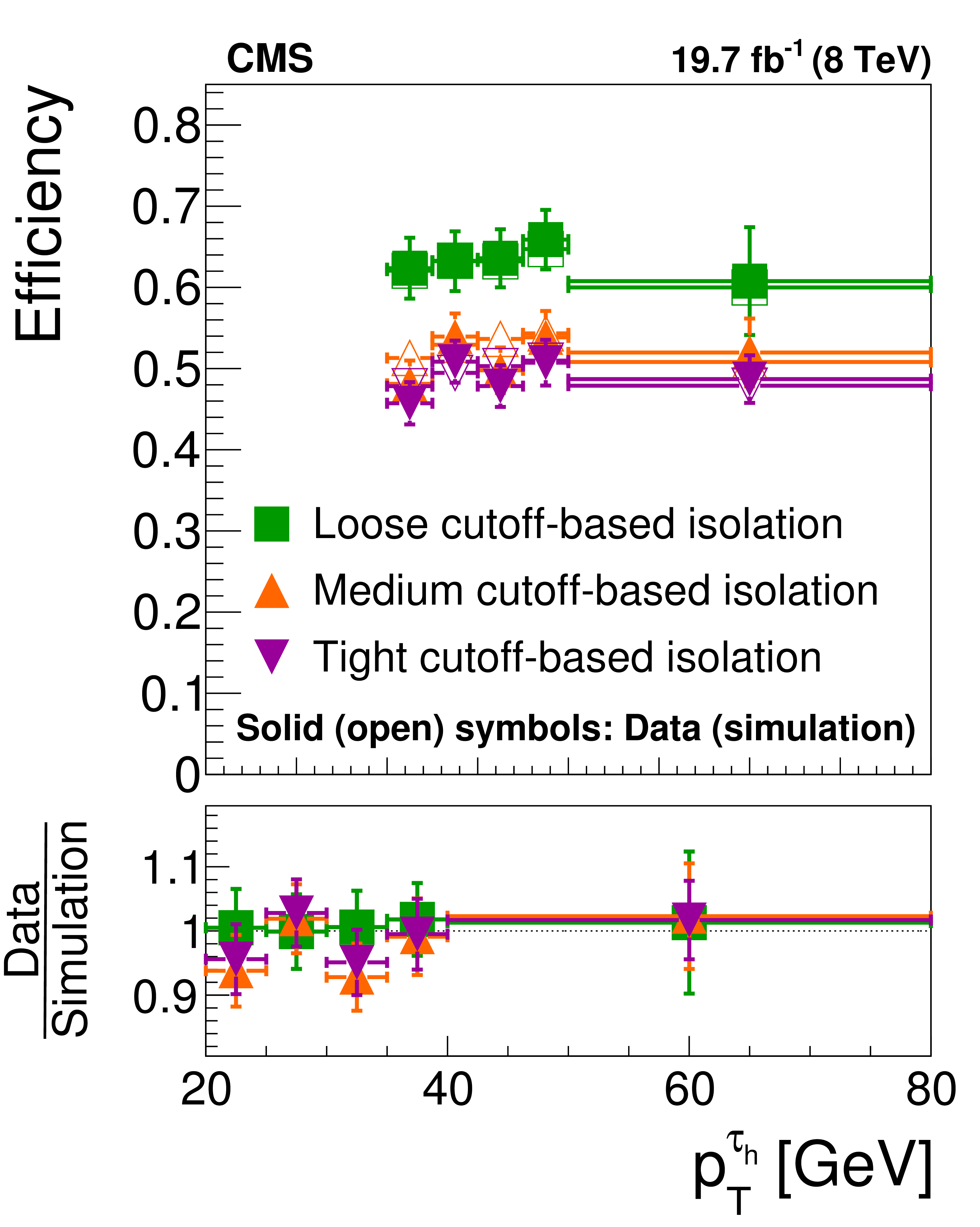
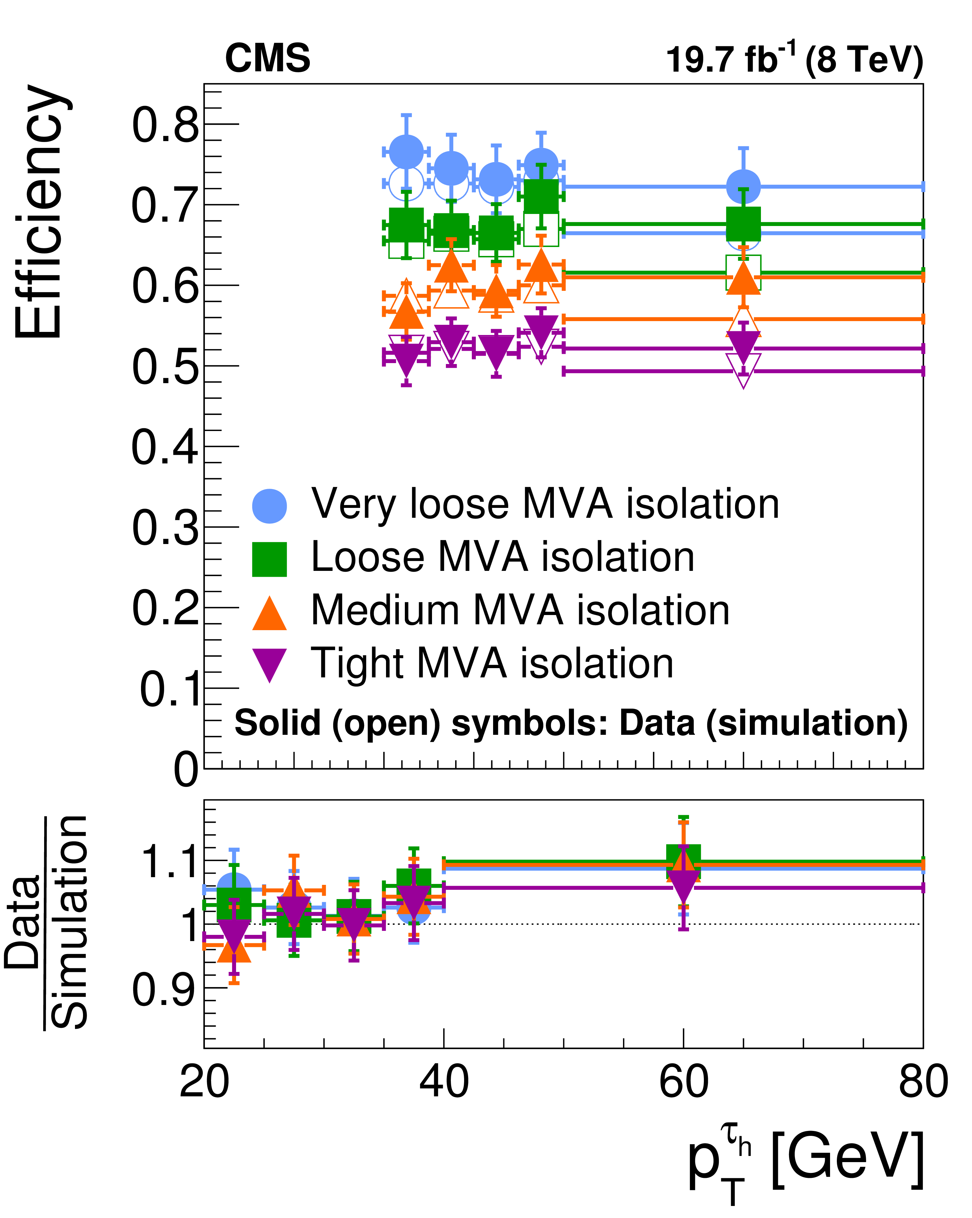
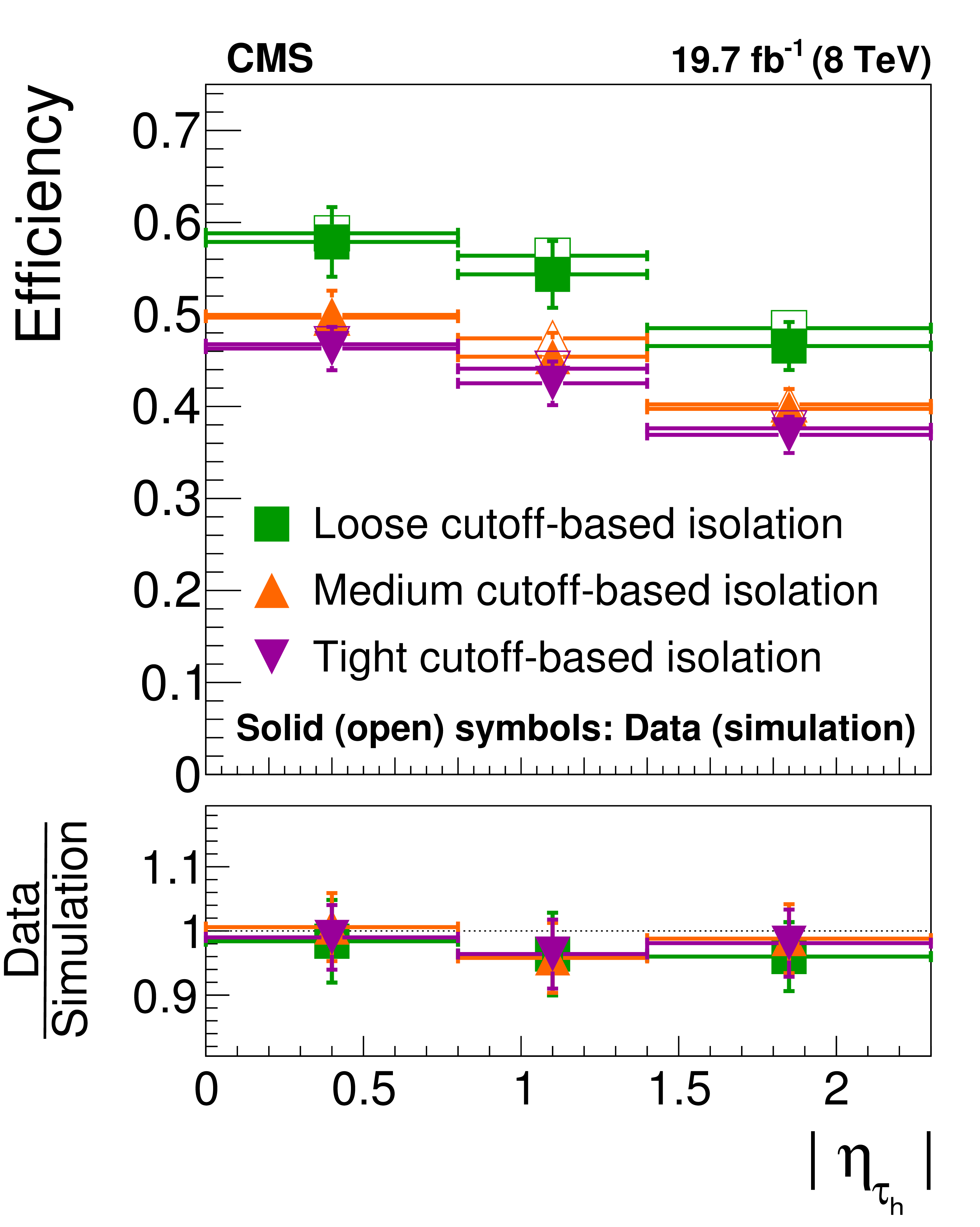
Figure 15-a:
Tau identification efficiency measured in $ {\mathrm {Z}}/ { {\gamma } ^{*}} \to {\tau } {\tau }\to {{\mu }} { {\tau }_{\mathrm {h}}} $ events as function of $ {p_{\mathrm {T}}} $ and $\eta $, for the cutoff-based and MVA-based $ { {\tau }_{\mathrm {h}}} $ isolation discriminants, compared to the MC expectation. The efficiency is computed relative to $ { {\tau }_{\mathrm {h}}} $ candidates passing the loose $ { {\tau }_{\mathrm {h}}} $ candidate selection described in Section 8.1. |
png pdf |
Figure 15-b:
Tau identification efficiency measured in $ {\mathrm {Z}}/ { {\gamma } ^{*}} \to {\tau } {\tau }\to {{\mu }} { {\tau }_{\mathrm {h}}} $ events as function of $ {p_{\mathrm {T}}} $ and $\eta $, for the cutoff-based and MVA-based $ { {\tau }_{\mathrm {h}}} $ isolation discriminants, compared to the MC expectation. The efficiency is computed relative to $ { {\tau }_{\mathrm {h}}} $ candidates passing the loose $ { {\tau }_{\mathrm {h}}} $ candidate selection described in Section 8.1. |
png pdf |
Figure 15-c:
Tau identification efficiency measured in $ {\mathrm {Z}}/ { {\gamma } ^{*}} \to {\tau } {\tau }\to {{\mu }} { {\tau }_{\mathrm {h}}} $ events as function of $ {p_{\mathrm {T}}} $ and $\eta $, for the cutoff-based and MVA-based $ { {\tau }_{\mathrm {h}}} $ isolation discriminants, compared to the MC expectation. The efficiency is computed relative to $ { {\tau }_{\mathrm {h}}} $ candidates passing the loose $ { {\tau }_{\mathrm {h}}} $ candidate selection described in Section 8.1. |

png pdf |
Figure 15-d:
Tau identification efficiency measured in $ {\mathrm {Z}}/ { {\gamma } ^{*}} \to {\tau } {\tau }\to {{\mu }} { {\tau }_{\mathrm {h}}} $ events as function of $ {p_{\mathrm {T}}} $ and $\eta $, for the cutoff-based and MVA-based $ { {\tau }_{\mathrm {h}}} $ isolation discriminants, compared to the MC expectation. The efficiency is computed relative to $ { {\tau }_{\mathrm {h}}} $ candidates passing the loose $ { {\tau }_{\mathrm {h}}} $ candidate selection described in Section 8.1. |

png pdf |
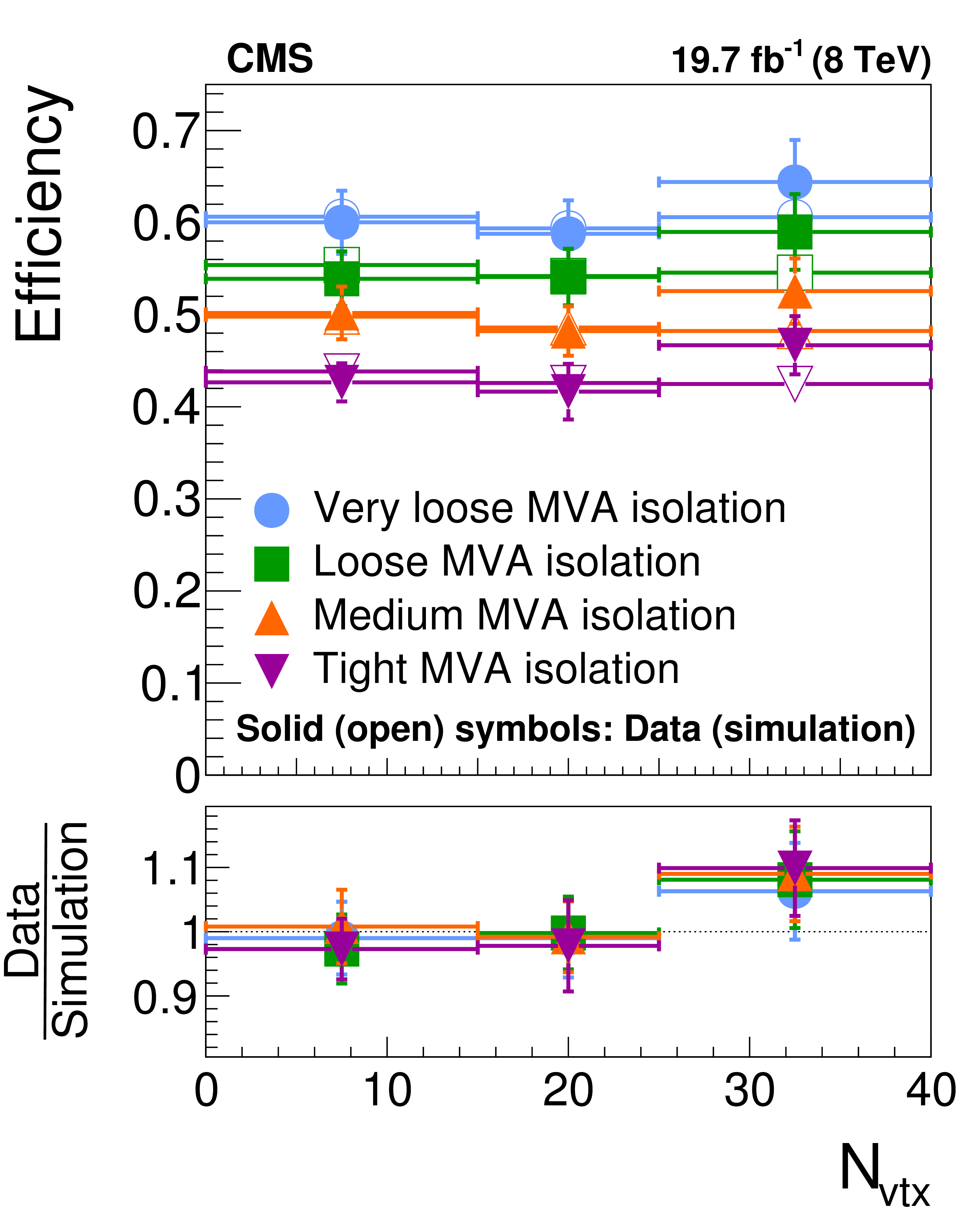
Figure 16-a:
Tau identification efficiency measured in $ {\mathrm {Z}}/ { {\gamma } ^{*}} \to {\tau } {\tau }\to {{\mu }} { {\tau }_{\mathrm {h}}} $ events as a function of the number of reconstructed vertices $ {N_{\text {vtx}}} $, for the cutoff-based and MVA-based $ { {\tau }_{\mathrm {h}}} $ isolation discriminants, compared to the MC expectation. The efficiency is computed relative to $ { {\tau }_{\mathrm {h}}} $ candidates passing the loose $ { {\tau }_{\mathrm {h}}} $ candidate selection described in Section 8.1. |
png pdf |
Figure 16-b:
Tau identification efficiency measured in $ {\mathrm {Z}}/ { {\gamma } ^{*}} \to {\tau } {\tau }\to {{\mu }} { {\tau }_{\mathrm {h}}} $ events as a function of the number of reconstructed vertices $ {N_{\text {vtx}}} $, for the cutoff-based and MVA-based $ { {\tau }_{\mathrm {h}}} $ isolation discriminants, compared to the MC expectation. The efficiency is computed relative to $ { {\tau }_{\mathrm {h}}} $ candidates passing the loose $ { {\tau }_{\mathrm {h}}} $ candidate selection described in Section 8.1. |
png pdf |
Figure 17-a:
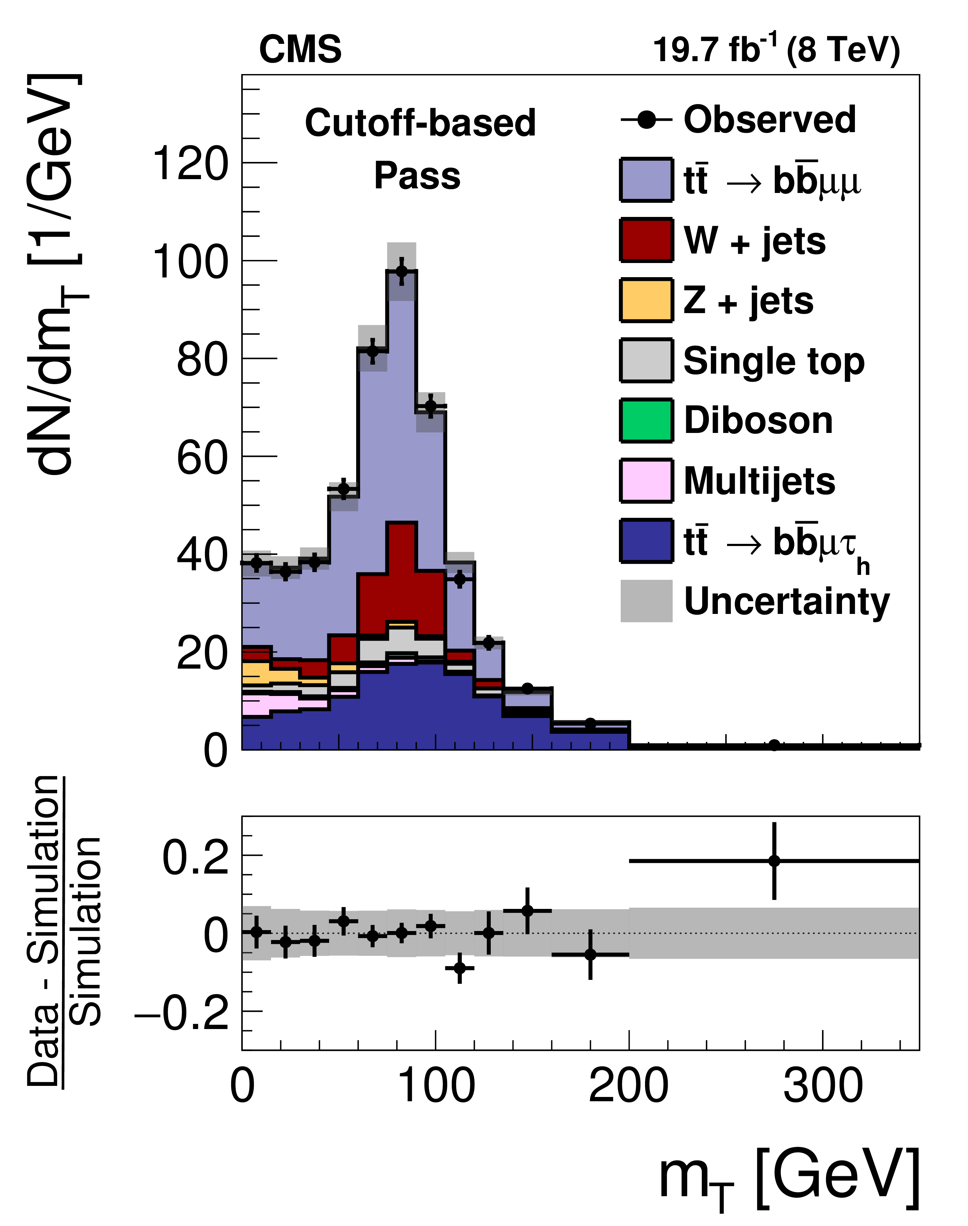
Distribution in the transverse mass of the muon and $ {E_{\mathrm {T}}^{\text {miss}}} $ in the pass region (a,c) and in the dimuon region (b,d) in $ {\mathrm {t}} {\overline {\mathrm {t}}}$ events used to measure the $ { {\tau }_{\mathrm {h}}} $ identification efficiency, for the loose WP of the cutoff-based (a,b) and MVA-based (c,d) $ { {\tau }_{\mathrm {h}}} $ isolation discriminants, respectively. The $ {\mathrm {t}} {\overline {\mathrm {t}}}$ events in which either the reconstructed muon or the reconstructed $ { {\tau }_{\mathrm {h}}} $ candidate are misidentified are denoted by ``$ {\mathrm {t}} {\overline {\mathrm {t}}}$ others''. The expected $ {m_{\mathrm {T}}} $ distribution is shown for the values of nuisance parameters obtained from the likelihood fit to the data, as described in Section 7.3. The ``Uncertainty'' band represents the statistical and systematic uncertainties added in quadrature. |

png pdf |
Figure 17-b:
Distribution in the transverse mass of the muon and $ {E_{\mathrm {T}}^{\text {miss}}} $ in the pass region (a,c) and in the dimuon region (b,d) in $ {\mathrm {t}} {\overline {\mathrm {t}}}$ events used to measure the $ { {\tau }_{\mathrm {h}}} $ identification efficiency, for the loose WP of the cutoff-based (a,b) and MVA-based (c,d) $ { {\tau }_{\mathrm {h}}} $ isolation discriminants, respectively. The $ {\mathrm {t}} {\overline {\mathrm {t}}}$ events in which either the reconstructed muon or the reconstructed $ { {\tau }_{\mathrm {h}}} $ candidate are misidentified are denoted by ``$ {\mathrm {t}} {\overline {\mathrm {t}}}$ others''. The expected $ {m_{\mathrm {T}}} $ distribution is shown for the values of nuisance parameters obtained from the likelihood fit to the data, as described in Section 7.3. The ``Uncertainty'' band represents the statistical and systematic uncertainties added in quadrature. |

png pdf |
Figure 17-c:
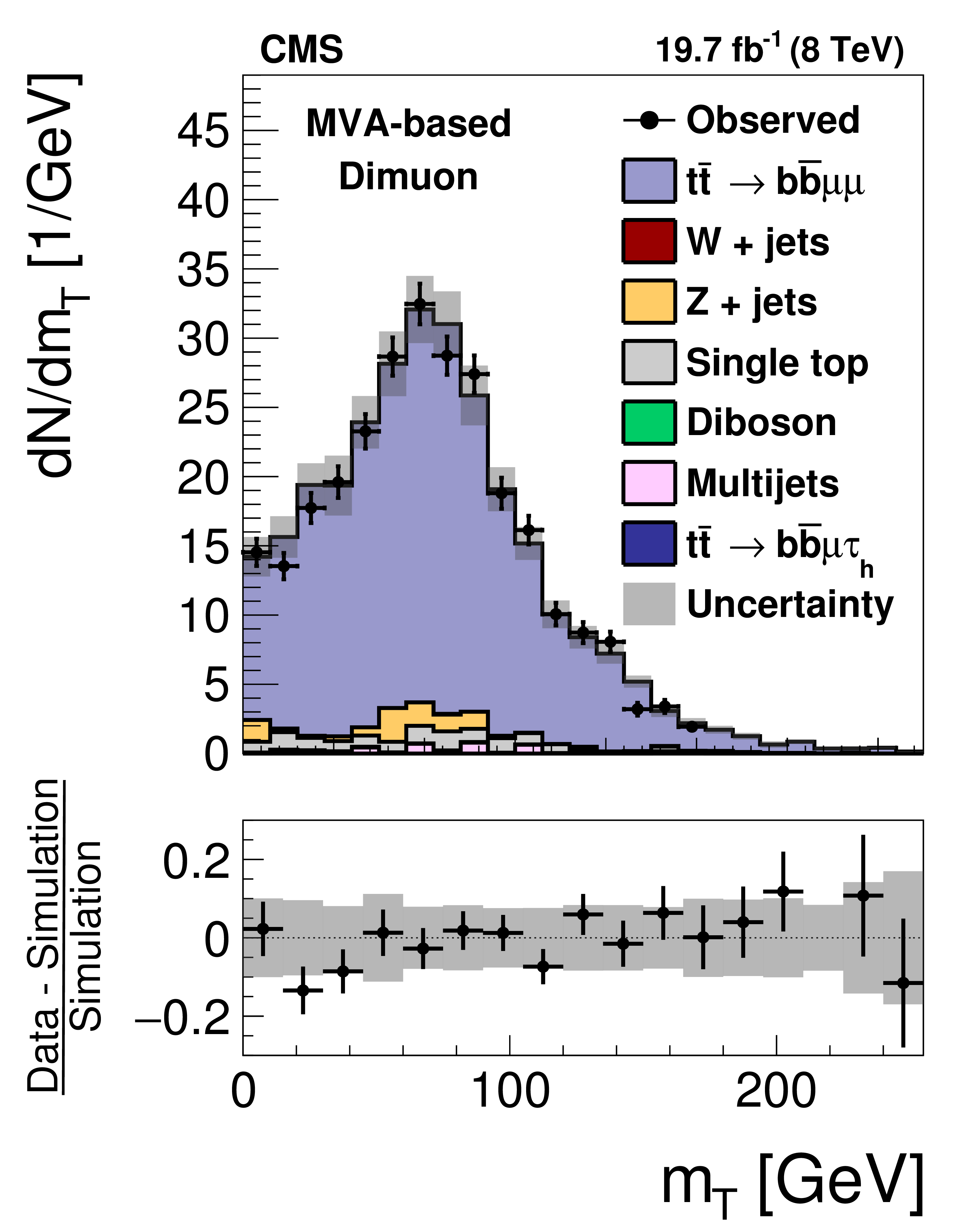
Distribution in the transverse mass of the muon and $ {E_{\mathrm {T}}^{\text {miss}}} $ in the pass region (a,c) and in the dimuon region (b,d) in $ {\mathrm {t}} {\overline {\mathrm {t}}}$ events used to measure the $ { {\tau }_{\mathrm {h}}} $ identification efficiency, for the loose WP of the cutoff-based (a,b) and MVA-based (c,d) $ { {\tau }_{\mathrm {h}}} $ isolation discriminants, respectively. The $ {\mathrm {t}} {\overline {\mathrm {t}}}$ events in which either the reconstructed muon or the reconstructed $ { {\tau }_{\mathrm {h}}} $ candidate are misidentified are denoted by ``$ {\mathrm {t}} {\overline {\mathrm {t}}}$ others''. The expected $ {m_{\mathrm {T}}} $ distribution is shown for the values of nuisance parameters obtained from the likelihood fit to the data, as described in Section 7.3. The ``Uncertainty'' band represents the statistical and systematic uncertainties added in quadrature. |
png pdf |
Figure 17-d:
Distribution in the transverse mass of the muon and $ {E_{\mathrm {T}}^{\text {miss}}} $ in the pass region (a,c) and in the dimuon region (b,d) in $ {\mathrm {t}} {\overline {\mathrm {t}}}$ events used to measure the $ { {\tau }_{\mathrm {h}}} $ identification efficiency, for the loose WP of the cutoff-based (a,b) and MVA-based (c,d) $ { {\tau }_{\mathrm {h}}} $ isolation discriminants, respectively. The $ {\mathrm {t}} {\overline {\mathrm {t}}}$ events in which either the reconstructed muon or the reconstructed $ { {\tau }_{\mathrm {h}}} $ candidate are misidentified are denoted by ``$ {\mathrm {t}} {\overline {\mathrm {t}}}$ others''. The expected $ {m_{\mathrm {T}}} $ distribution is shown for the values of nuisance parameters obtained from the likelihood fit to the data, as described in Section 7.3. The ``Uncertainty'' band represents the statistical and systematic uncertainties added in quadrature. |
png pdf |
Figure 18-a:
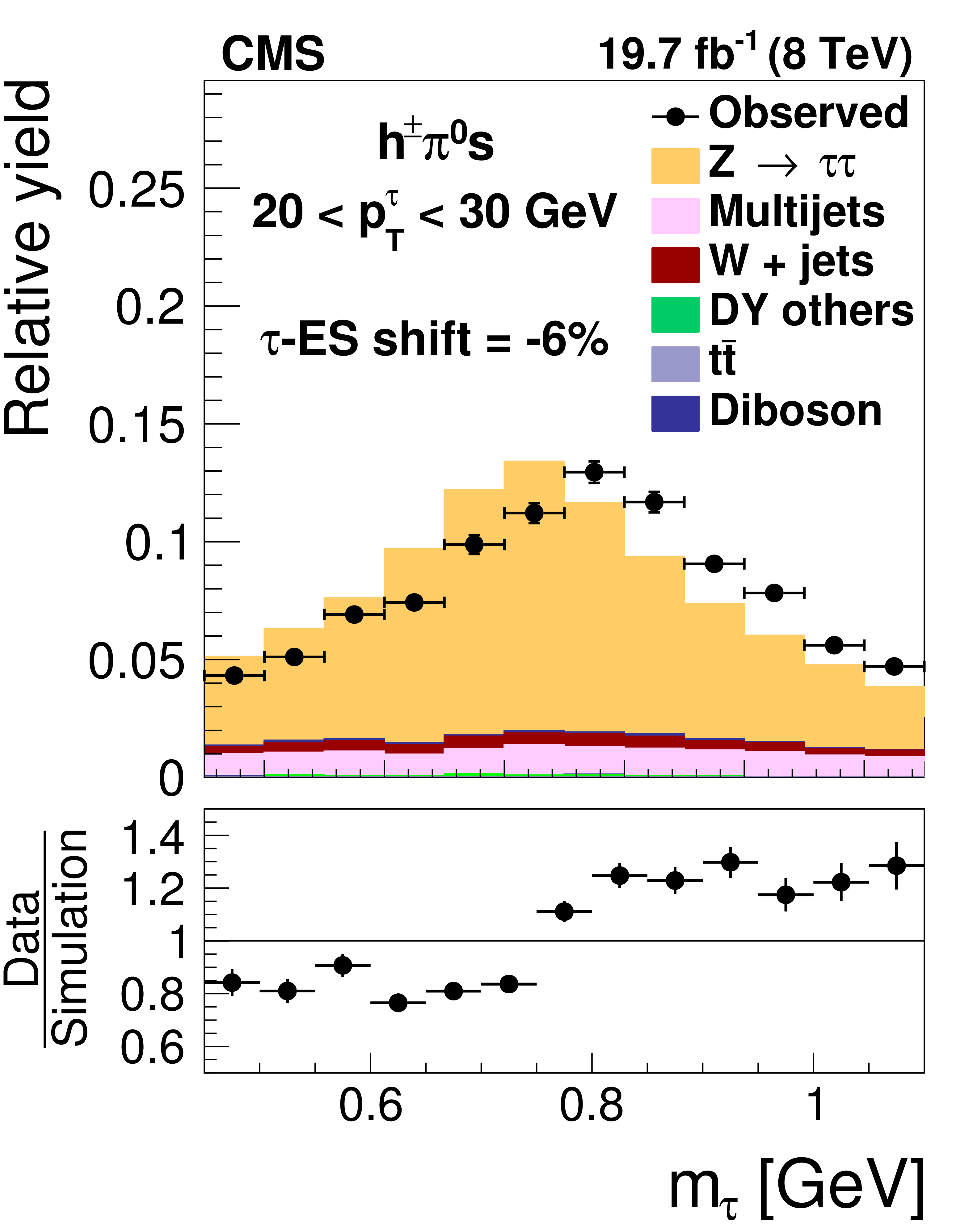
Distribution in $m_{ { {\tau }_{\mathrm {h}}} }$, observed in events containing $ { {\tau }_{\mathrm {h}}} $ candidates of 20 $< {p_{\mathrm {T}}} <$ 30 GeV, reconstructed in the decay modes $ {\mathrm {h}^{\pm } { {\pi ^0}}\text {s}} $ (a,b,c) and $ {\mathrm {h}^{\pm }\mathrm {h}^{\mp }\mathrm {h}^{\pm }} $ (d,e,f), compared to the sum of $ {\mathrm {Z}}/ { {\gamma } ^{*}} \to {\tau } {\tau }$ signal plus background expectation. The $m_{ { {\tau }_{\mathrm {h}}} }$ shape templates for the $ {\mathrm {Z}}/ { {\gamma } ^{*}} \to {\tau } {\tau }$ signal are shown for $ {\tau }$ES variations of $-6%$ (a,d), 0% (b,e) and $+6%$ (c,f). For clarity, the symbols $ {p_{\mathrm {T}}} ^{ {\tau }}$ and $m_{ {\tau }}$ are used instead of $ {p_{\mathrm {T}}} ^{ { {\tau }_{\mathrm {h}}} }$ and $m_{ { {\tau }_{\mathrm {h}}} }$ in these plots. |
png pdf |
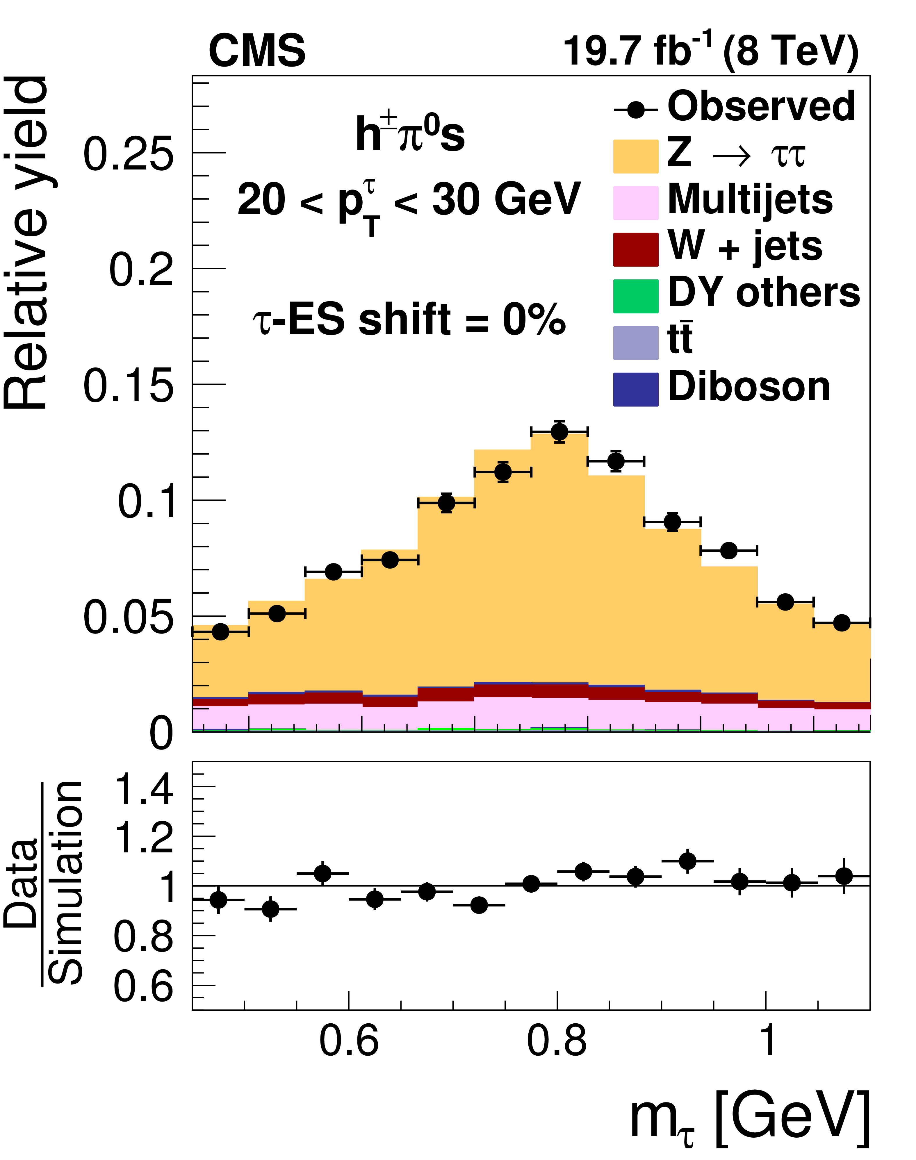
Figure 18-b:
Distribution in $m_{ { {\tau }_{\mathrm {h}}} }$, observed in events containing $ { {\tau }_{\mathrm {h}}} $ candidates of 20 $< {p_{\mathrm {T}}} <$ 30 GeV, reconstructed in the decay modes $ {\mathrm {h}^{\pm } { {\pi ^0}}\text {s}} $ (a,b,c) and $ {\mathrm {h}^{\pm }\mathrm {h}^{\mp }\mathrm {h}^{\pm }} $ (d,e,f), compared to the sum of $ {\mathrm {Z}}/ { {\gamma } ^{*}} \to {\tau } {\tau }$ signal plus background expectation. The $m_{ { {\tau }_{\mathrm {h}}} }$ shape templates for the $ {\mathrm {Z}}/ { {\gamma } ^{*}} \to {\tau } {\tau }$ signal are shown for $ {\tau }$ES variations of $-6%$ (a,d), 0% (b,e) and $+6%$ (c,f). For clarity, the symbols $ {p_{\mathrm {T}}} ^{ {\tau }}$ and $m_{ {\tau }}$ are used instead of $ {p_{\mathrm {T}}} ^{ { {\tau }_{\mathrm {h}}} }$ and $m_{ { {\tau }_{\mathrm {h}}} }$ in these plots. |

png pdf |
Figure 18-c:
Distribution in $m_{ { {\tau }_{\mathrm {h}}} }$, observed in events containing $ { {\tau }_{\mathrm {h}}} $ candidates of 20 $< {p_{\mathrm {T}}} <$ 30 GeV, reconstructed in the decay modes $ {\mathrm {h}^{\pm } { {\pi ^0}}\text {s}} $ (a,b,c) and $ {\mathrm {h}^{\pm }\mathrm {h}^{\mp }\mathrm {h}^{\pm }} $ (d,e,f), compared to the sum of $ {\mathrm {Z}}/ { {\gamma } ^{*}} \to {\tau } {\tau }$ signal plus background expectation. The $m_{ { {\tau }_{\mathrm {h}}} }$ shape templates for the $ {\mathrm {Z}}/ { {\gamma } ^{*}} \to {\tau } {\tau }$ signal are shown for $ {\tau }$ES variations of $-6%$ (a,d), 0% (b,e) and $+6%$ (c,f). For clarity, the symbols $ {p_{\mathrm {T}}} ^{ {\tau }}$ and $m_{ {\tau }}$ are used instead of $ {p_{\mathrm {T}}} ^{ { {\tau }_{\mathrm {h}}} }$ and $m_{ { {\tau }_{\mathrm {h}}} }$ in these plots. |
png pdf |
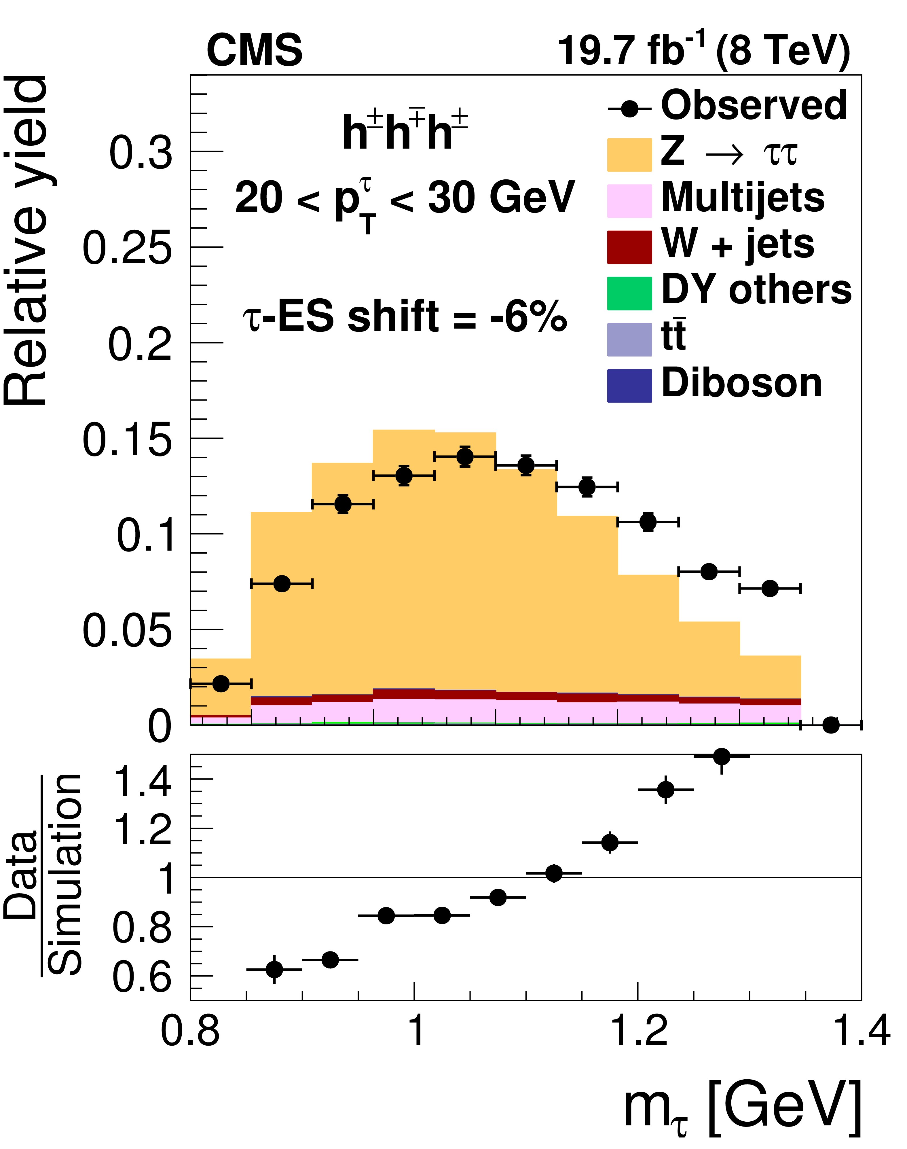
Figure 18-d:
Distribution in $m_{ { {\tau }_{\mathrm {h}}} }$, observed in events containing $ { {\tau }_{\mathrm {h}}} $ candidates of 20 $< {p_{\mathrm {T}}} <$ 30 GeV, reconstructed in the decay modes $ {\mathrm {h}^{\pm } { {\pi ^0}}\text {s}} $ (a,b,c) and $ {\mathrm {h}^{\pm }\mathrm {h}^{\mp }\mathrm {h}^{\pm }} $ (d,e,f), compared to the sum of $ {\mathrm {Z}}/ { {\gamma } ^{*}} \to {\tau } {\tau }$ signal plus background expectation. The $m_{ { {\tau }_{\mathrm {h}}} }$ shape templates for the $ {\mathrm {Z}}/ { {\gamma } ^{*}} \to {\tau } {\tau }$ signal are shown for $ {\tau }$ES variations of $-6%$ (a,d), 0% (b,e) and $+6%$ (c,f). For clarity, the symbols $ {p_{\mathrm {T}}} ^{ {\tau }}$ and $m_{ {\tau }}$ are used instead of $ {p_{\mathrm {T}}} ^{ { {\tau }_{\mathrm {h}}} }$ and $m_{ { {\tau }_{\mathrm {h}}} }$ in these plots. |

png pdf |
Figure 18-e:
Distribution in $m_{ { {\tau }_{\mathrm {h}}} }$, observed in events containing $ { {\tau }_{\mathrm {h}}} $ candidates of 20 $< {p_{\mathrm {T}}} <$ 30 GeV, reconstructed in the decay modes $ {\mathrm {h}^{\pm } { {\pi ^0}}\text {s}} $ (a,b,c) and $ {\mathrm {h}^{\pm }\mathrm {h}^{\mp }\mathrm {h}^{\pm }} $ (d,e,f), compared to the sum of $ {\mathrm {Z}}/ { {\gamma } ^{*}} \to {\tau } {\tau }$ signal plus background expectation. The $m_{ { {\tau }_{\mathrm {h}}} }$ shape templates for the $ {\mathrm {Z}}/ { {\gamma } ^{*}} \to {\tau } {\tau }$ signal are shown for $ {\tau }$ES variations of $-6%$ (a,d), 0% (b,e) and $+6%$ (c,f). For clarity, the symbols $ {p_{\mathrm {T}}} ^{ {\tau }}$ and $m_{ {\tau }}$ are used instead of $ {p_{\mathrm {T}}} ^{ { {\tau }_{\mathrm {h}}} }$ and $m_{ { {\tau }_{\mathrm {h}}} }$ in these plots. |
png pdf |
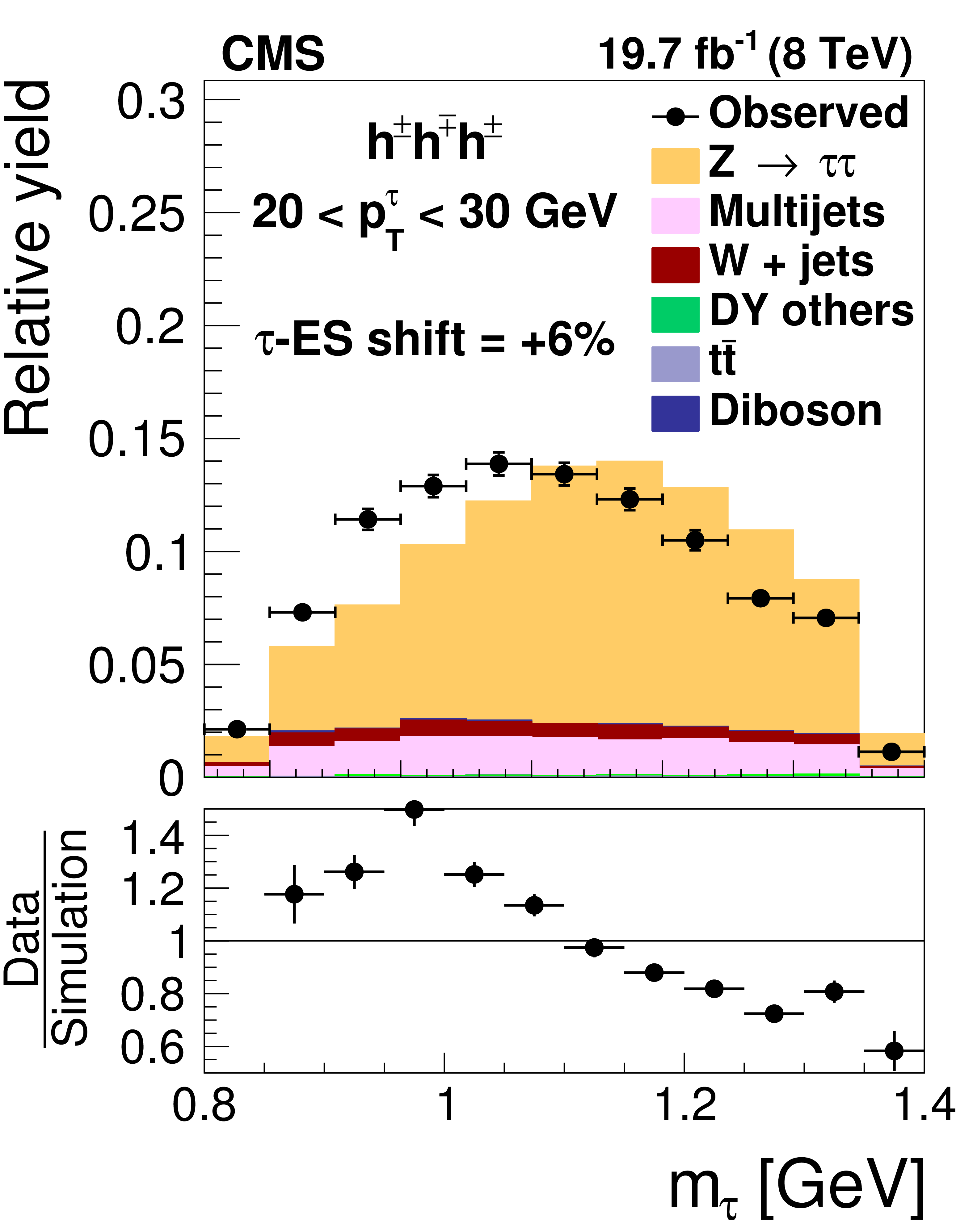
Figure 18-f:
Distribution in $m_{ { {\tau }_{\mathrm {h}}} }$, observed in events containing $ { {\tau }_{\mathrm {h}}} $ candidates of 20 $< {p_{\mathrm {T}}} <$ 30 GeV, reconstructed in the decay modes $ {\mathrm {h}^{\pm } { {\pi ^0}}\text {s}} $ (a,b,c) and $ {\mathrm {h}^{\pm }\mathrm {h}^{\mp }\mathrm {h}^{\pm }} $ (d,e,f), compared to the sum of $ {\mathrm {Z}}/ { {\gamma } ^{*}} \to {\tau } {\tau }$ signal plus background expectation. The $m_{ { {\tau }_{\mathrm {h}}} }$ shape templates for the $ {\mathrm {Z}}/ { {\gamma } ^{*}} \to {\tau } {\tau }$ signal are shown for $ {\tau }$ES variations of $-6%$ (a,d), 0% (b,e) and $+6%$ (c,f). For clarity, the symbols $ {p_{\mathrm {T}}} ^{ {\tau }}$ and $m_{ {\tau }}$ are used instead of $ {p_{\mathrm {T}}} ^{ { {\tau }_{\mathrm {h}}} }$ and $m_{ { {\tau }_{\mathrm {h}}} }$ in these plots. |
png pdf |
Figure 19-a:
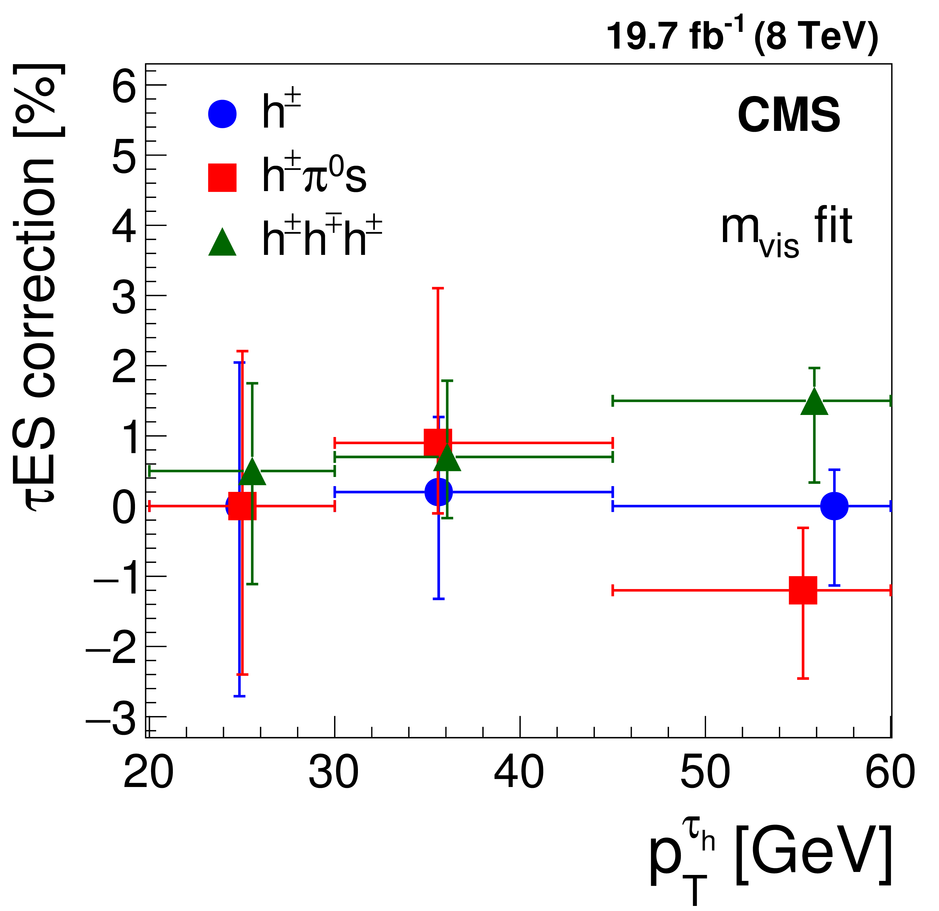
Energy scale corrections for $ { {\tau }_{\mathrm {h}}} $ measured in $ {\mathrm {Z}}/ { {\gamma } ^{*}} \to {\tau } {\tau }$ events, using the distribution in (a) visible mass of muon and $ { {\tau }_{\mathrm {h}}} $ and (b) of the $ { {\tau }_{\mathrm {h}}} $ candidate mass, for $ { {\tau }_{\mathrm {h}}} $ reconstructed in different decay modes and in different ranges of $ { {\tau }_{\mathrm {h}}} $ candidate $ {p_{\mathrm {T}}} $. |
png pdf |
Figure 19-b:
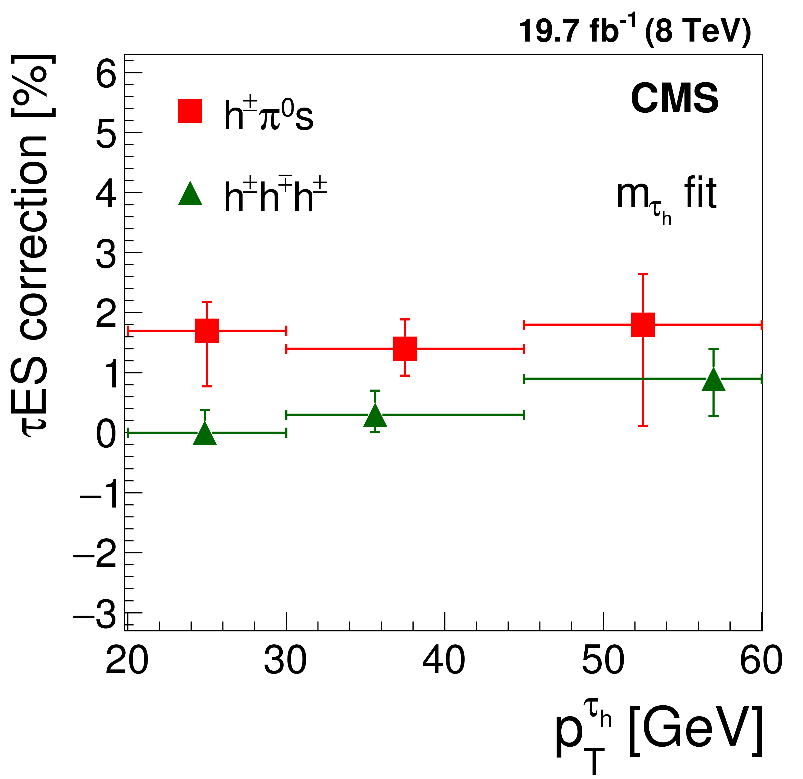
Energy scale corrections for $ { {\tau }_{\mathrm {h}}} $ measured in $ {\mathrm {Z}}/ { {\gamma } ^{*}} \to {\tau } {\tau }$ events, using the distribution in (a) visible mass of muon and $ { {\tau }_{\mathrm {h}}} $ and (b) of the $ { {\tau }_{\mathrm {h}}} $ candidate mass, for $ { {\tau }_{\mathrm {h}}} $ reconstructed in different decay modes and in different ranges of $ { {\tau }_{\mathrm {h}}} $ candidate $ {p_{\mathrm {T}}} $. |
png pdf |
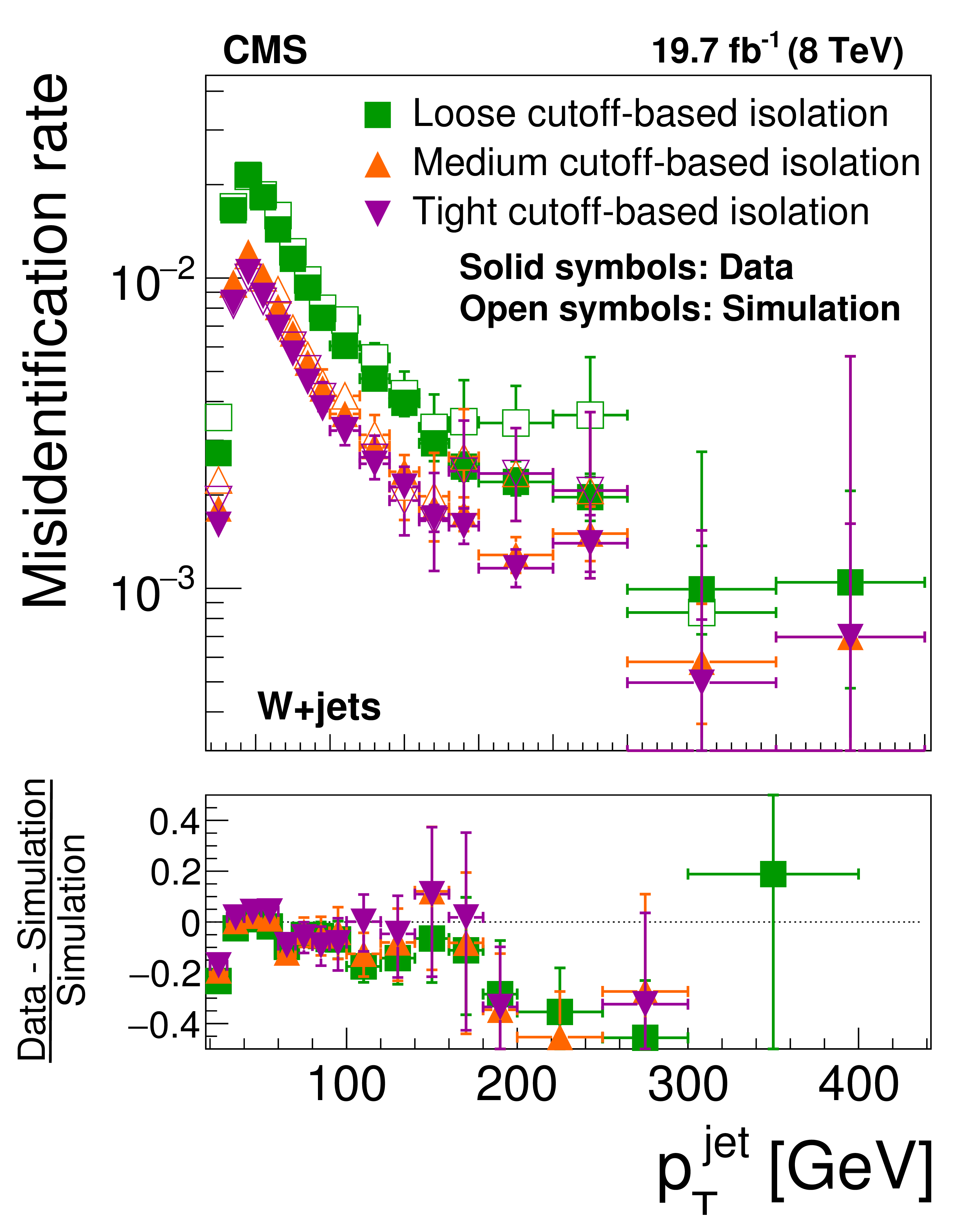
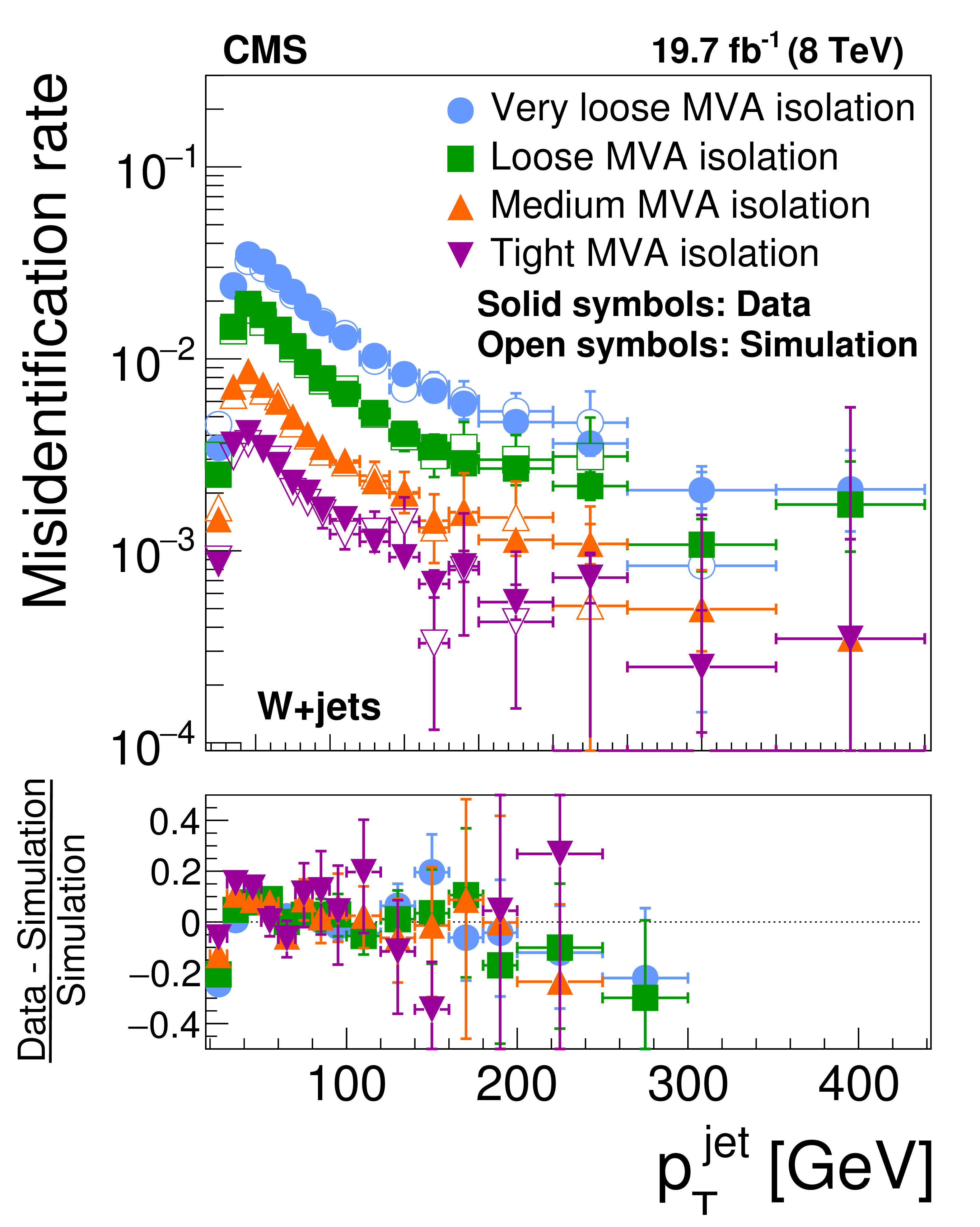
Figure 20-a:
Probabilities for quark and gluon jets in W+jets (a,b) and multijet (c,d) events to pass the cutoff-based (a,c) and MVA-based (b,d) $ { {\tau }_{\mathrm {h}}} $ isolation discriminant, as a function of jet $ {p_{\mathrm {T}}} $. The misidentification rates measured in the data are compared to the MC expectation. |
png pdf |
Figure 20-b:
Probabilities for quark and gluon jets in W+jets (a,b) and multijet (c,d) events to pass the cutoff-based (a,c) and MVA-based (b,d) $ { {\tau }_{\mathrm {h}}} $ isolation discriminant, as a function of jet $ {p_{\mathrm {T}}} $. The misidentification rates measured in the data are compared to the MC expectation. |
png pdf |
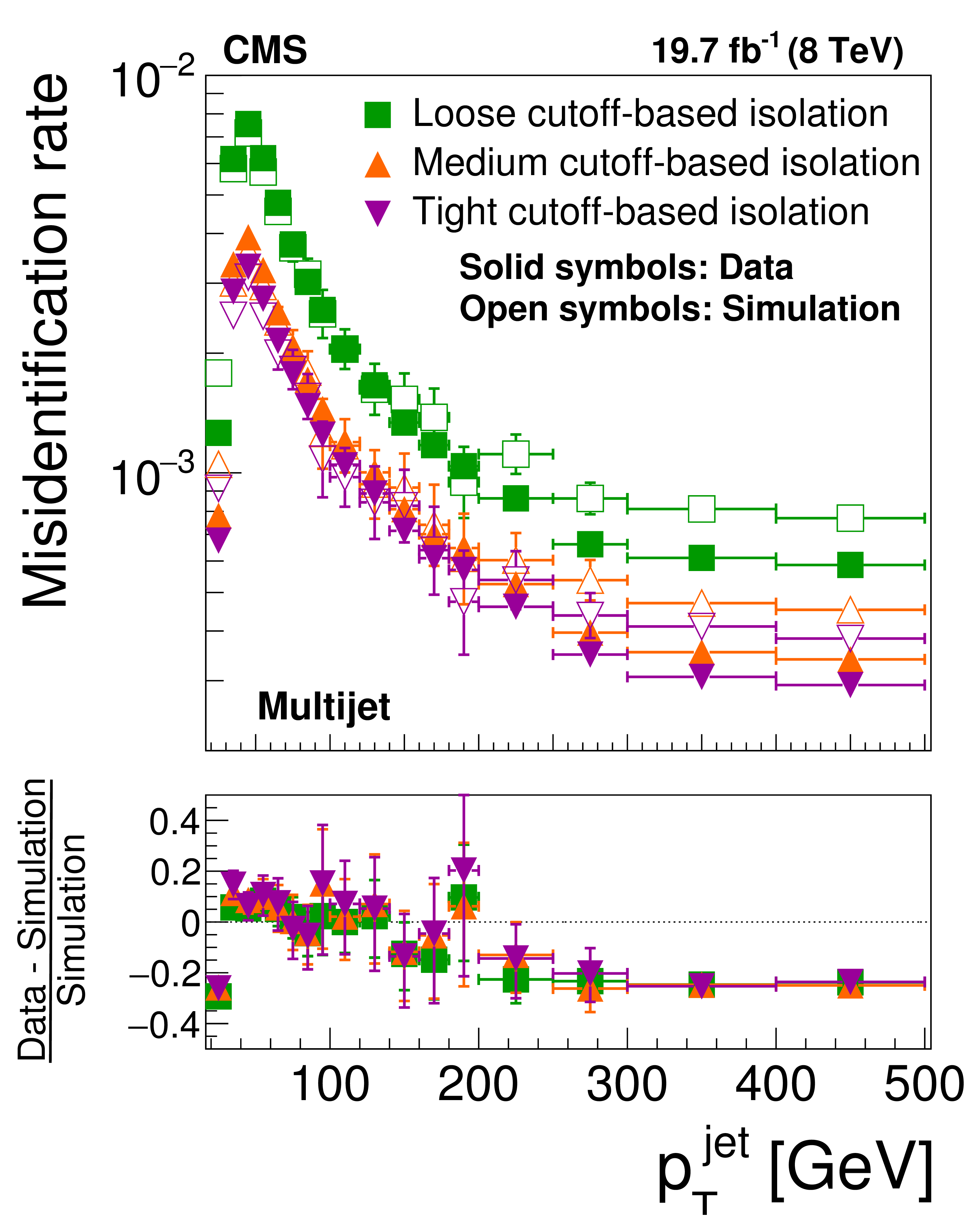
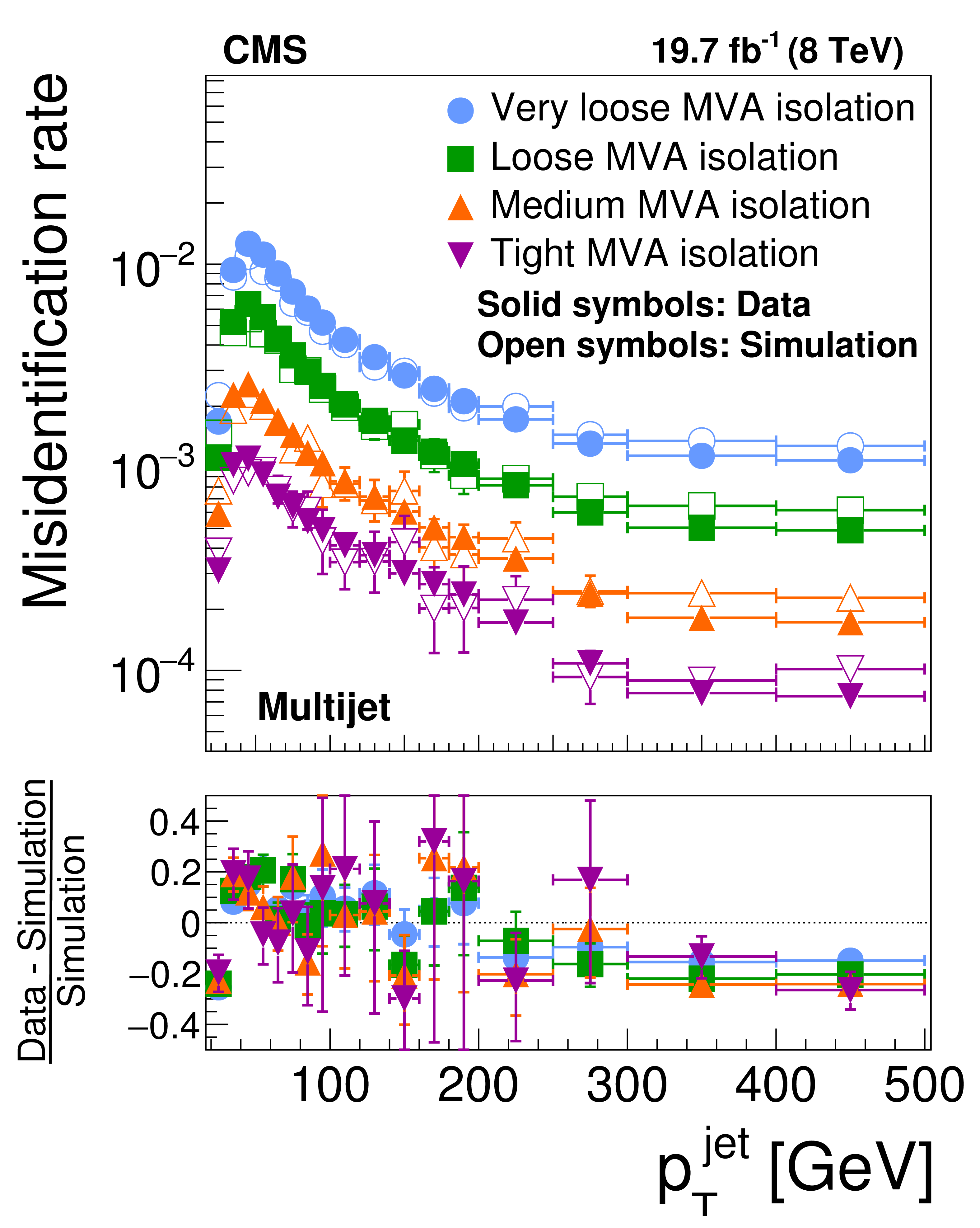
Figure 20-c:
Probabilities for quark and gluon jets in W+jets (a,b) and multijet (c,d) events to pass the cutoff-based (a,c) and MVA-based (b,d) $ { {\tau }_{\mathrm {h}}} $ isolation discriminant, as a function of jet $ {p_{\mathrm {T}}} $. The misidentification rates measured in the data are compared to the MC expectation. |
png pdf |
Figure 20-d:
Probabilities for quark and gluon jets in W+jets (a,b) and multijet (c,d) events to pass the cutoff-based (a,c) and MVA-based (b,d) $ { {\tau }_{\mathrm {h}}} $ isolation discriminant, as a function of jet $ {p_{\mathrm {T}}} $. The misidentification rates measured in the data are compared to the MC expectation. |
png pdf |
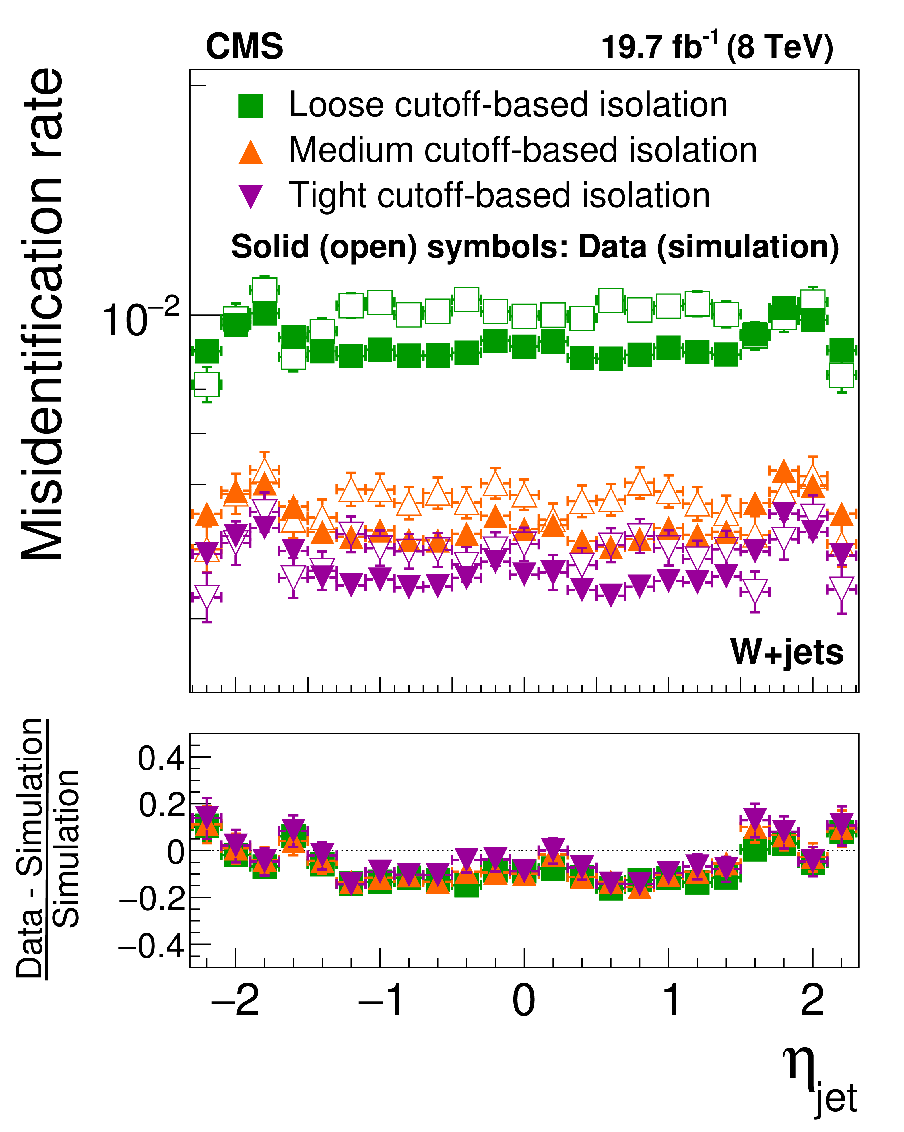
Figure 21-a:
Probabilities for quark and gluon jets in W+jets (a,b) and multijet (c,d) events to pass the cutoff-based (a,c) and MVA-based (b,d) $ { {\tau }_{\mathrm {h}}} $ isolation discriminant, as a function of jet $\eta $. The misidentification rates measured in the data are compared to the MC expectation. |

png pdf |
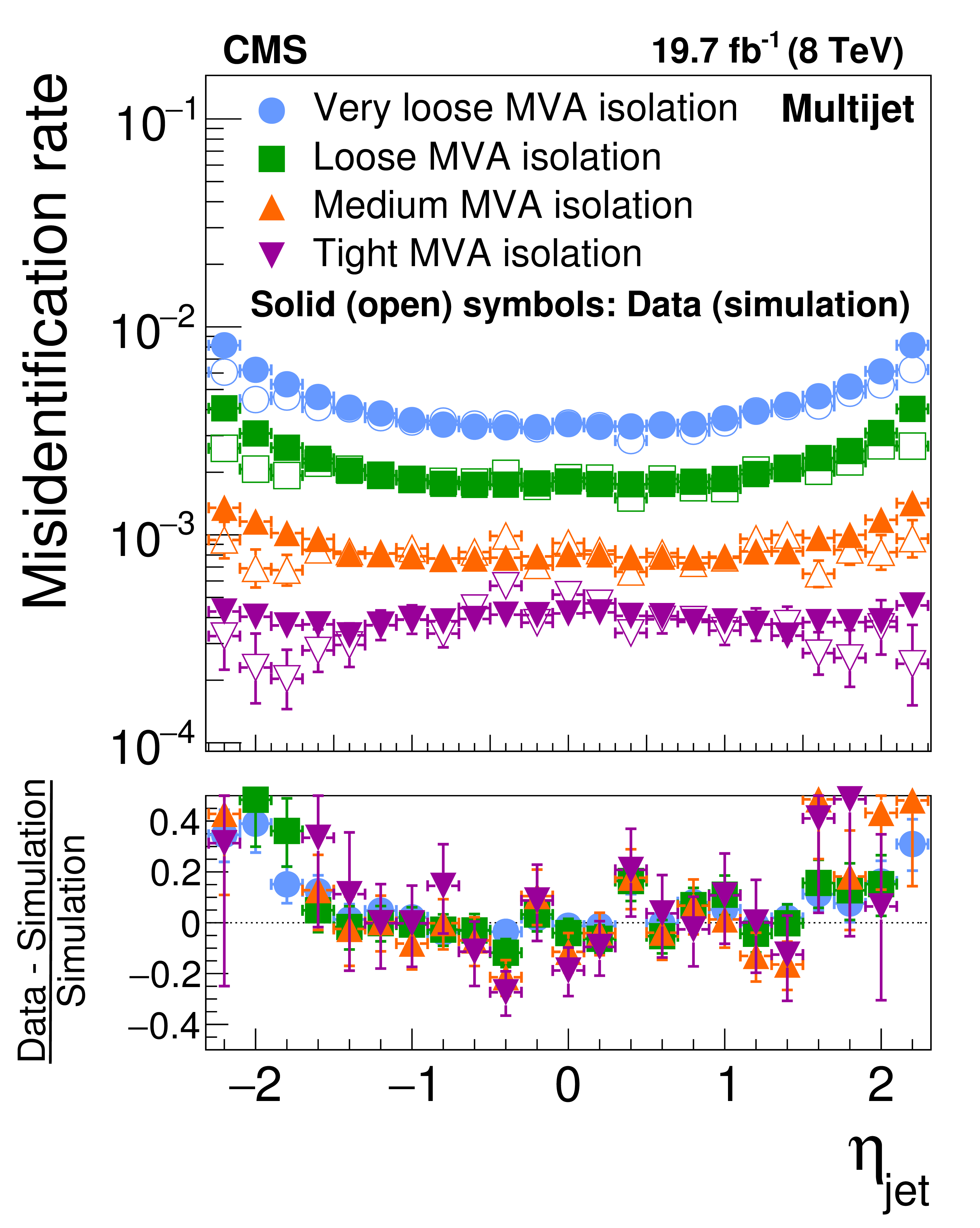
Figure 21-b:
Probabilities for quark and gluon jets in W+jets (a,b) and multijet (c,d) events to pass the cutoff-based (a,c) and MVA-based (b,d) $ { {\tau }_{\mathrm {h}}} $ isolation discriminant, as a function of jet $\eta $. The misidentification rates measured in the data are compared to the MC expectation. |

png pdf |
Figure 21-c:
Probabilities for quark and gluon jets in W+jets (a,b) and multijet (c,d) events to pass the cutoff-based (a,c) and MVA-based (b,d) $ { {\tau }_{\mathrm {h}}} $ isolation discriminant, as a function of jet $\eta $. The misidentification rates measured in the data are compared to the MC expectation. |
png pdf |
Figure 21-d:
Probabilities for quark and gluon jets in W+jets (a,b) and multijet (c,d) events to pass the cutoff-based (a,c) and MVA-based (b,d) $ { {\tau }_{\mathrm {h}}} $ isolation discriminant, as a function of jet $\eta $. The misidentification rates measured in the data are compared to the MC expectation. |
png pdf |
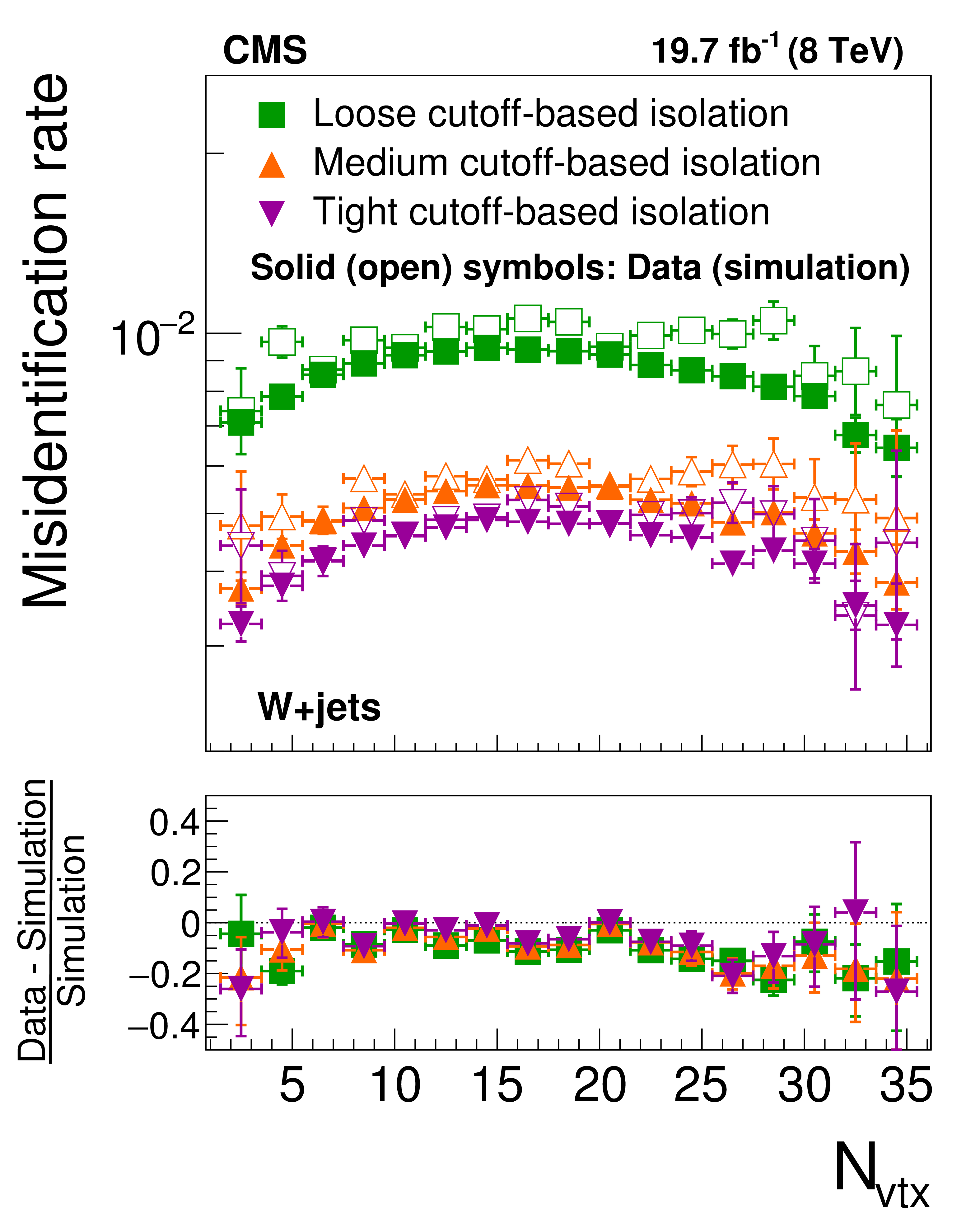
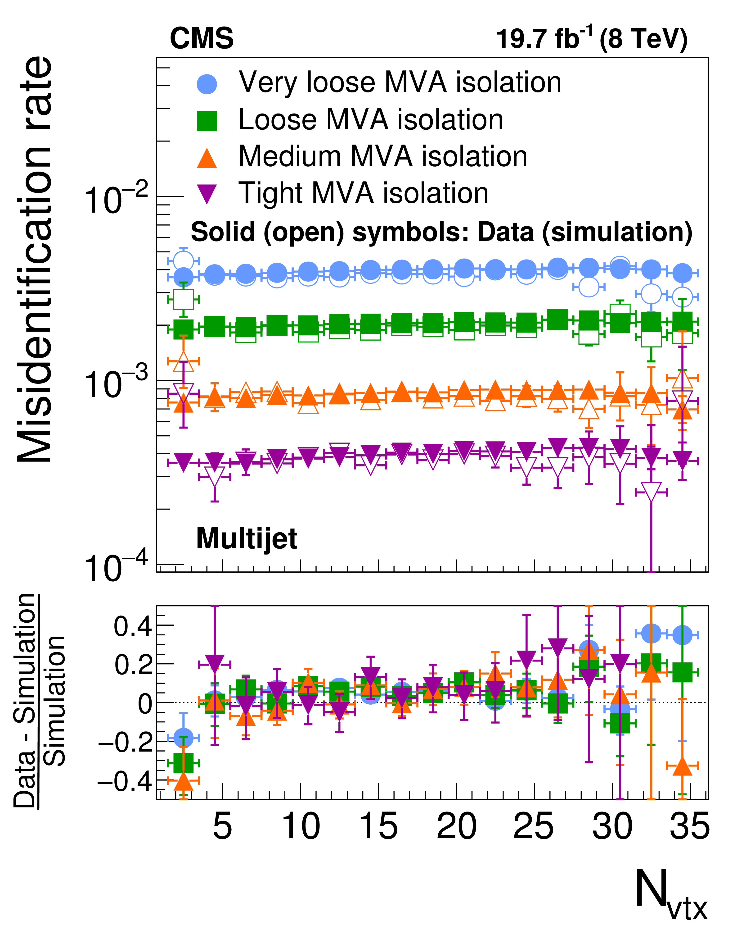
Figure 22-a:
Probabilities for quark and gluon jets in W+jets (a,b) and multijet (c,d) events to pass the cutoff-based (a,c) and MVA-based (b,d) $ { {\tau }_{\mathrm {h}}} $ isolation discriminant, as a function of $ {N_{\text {vtx}}} $. The misidentification rates measured in the data are compared to the MC expectation. |
png pdf |
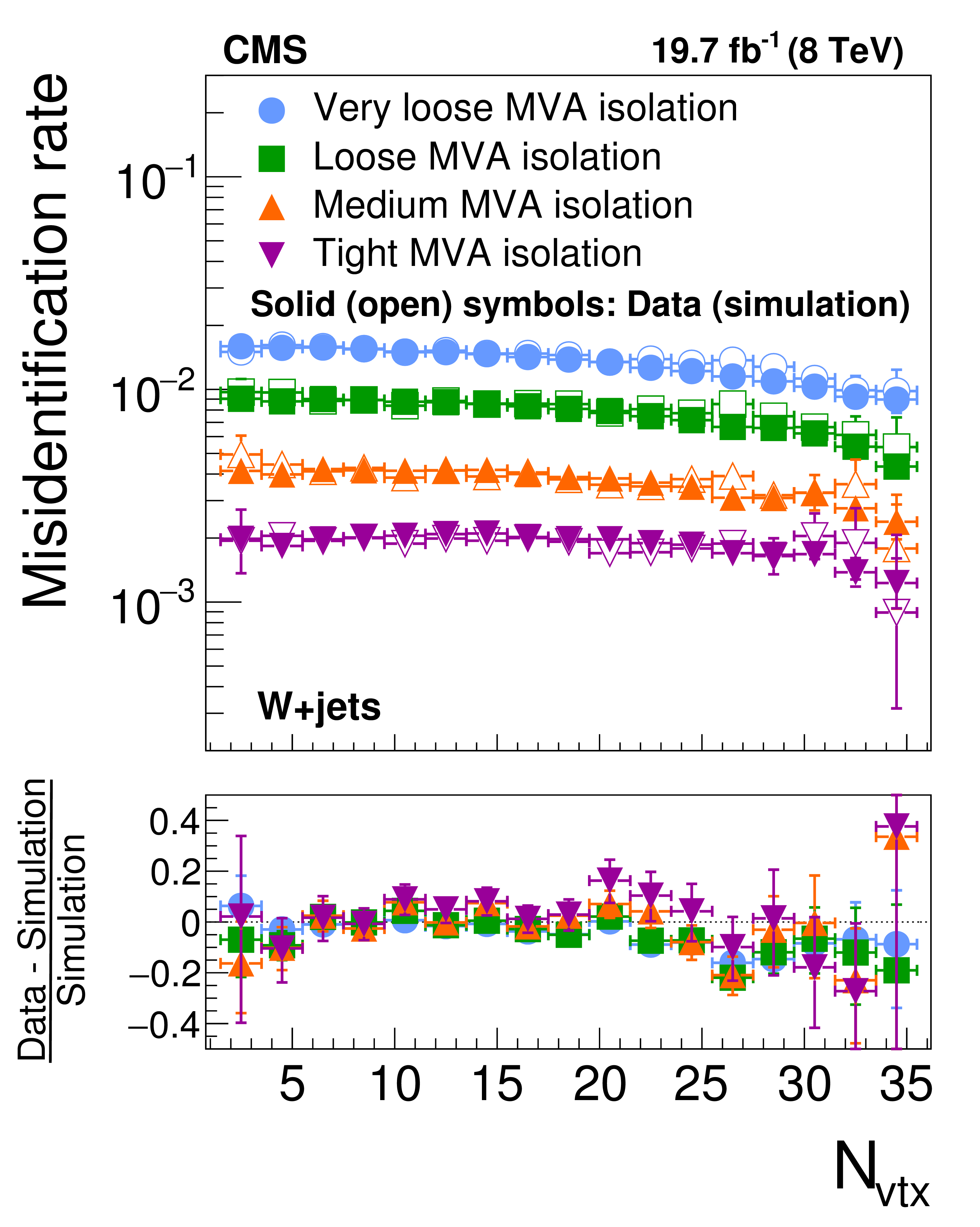
Figure 22-b:
Probabilities for quark and gluon jets in W+jets (a,b) and multijet (c,d) events to pass the cutoff-based (a,c) and MVA-based (b,d) $ { {\tau }_{\mathrm {h}}} $ isolation discriminant, as a function of $ {N_{\text {vtx}}} $. The misidentification rates measured in the data are compared to the MC expectation. |

png pdf |
Figure 22-c:
Probabilities for quark and gluon jets in W+jets (a,b) and multijet (c,d) events to pass the cutoff-based (a,c) and MVA-based (b,d) $ { {\tau }_{\mathrm {h}}} $ isolation discriminant, as a function of $ {N_{\text {vtx}}} $. The misidentification rates measured in the data are compared to the MC expectation. |
png pdf |
Figure 22-d:
Probabilities for quark and gluon jets in W+jets (a,b) and multijet (c,d) events to pass the cutoff-based (a,c) and MVA-based (b,d) $ { {\tau }_{\mathrm {h}}} $ isolation discriminant, as a function of $ {N_{\text {vtx}}} $. The misidentification rates measured in the data are compared to the MC expectation. |
png pdf |
Figure 23-a:
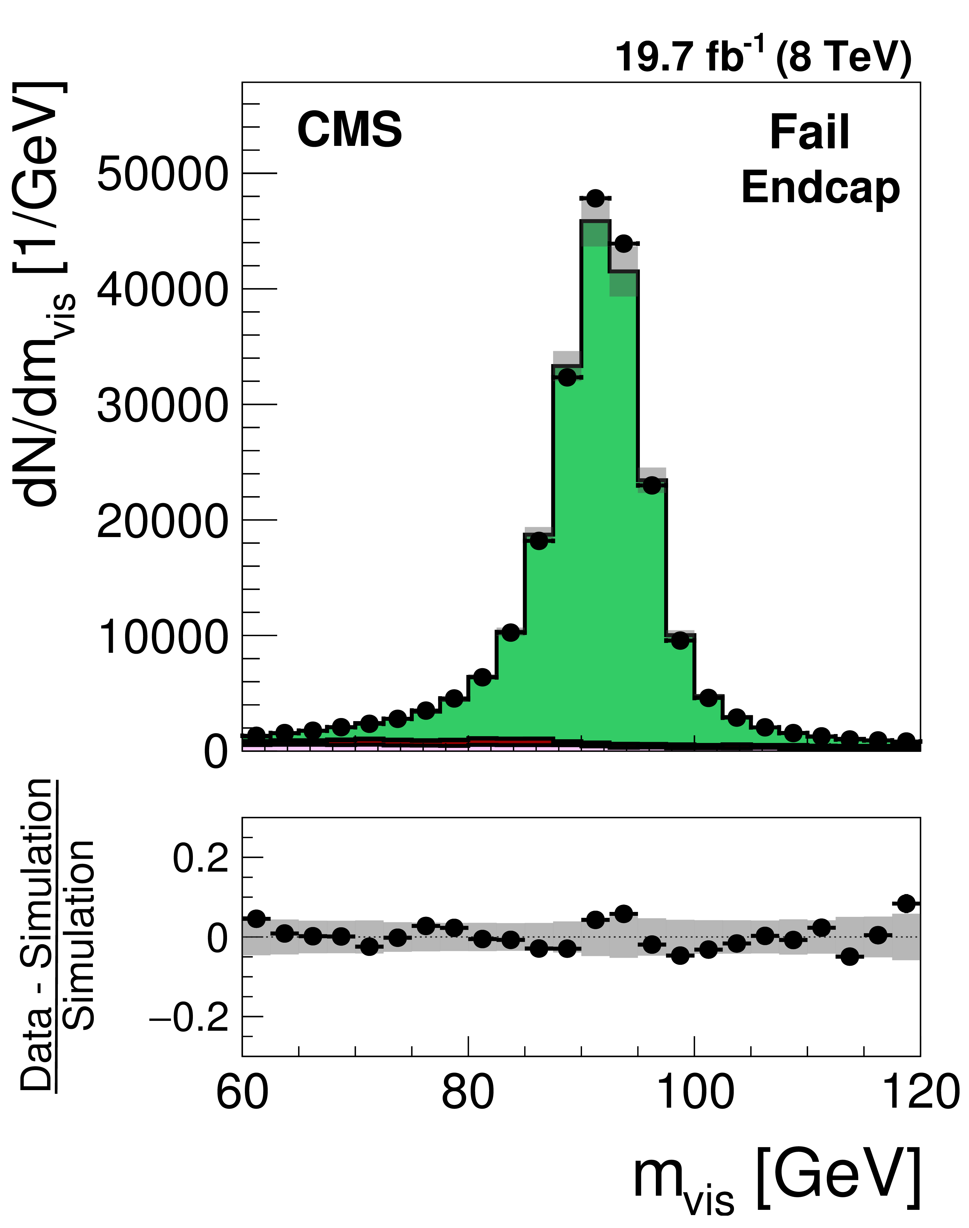
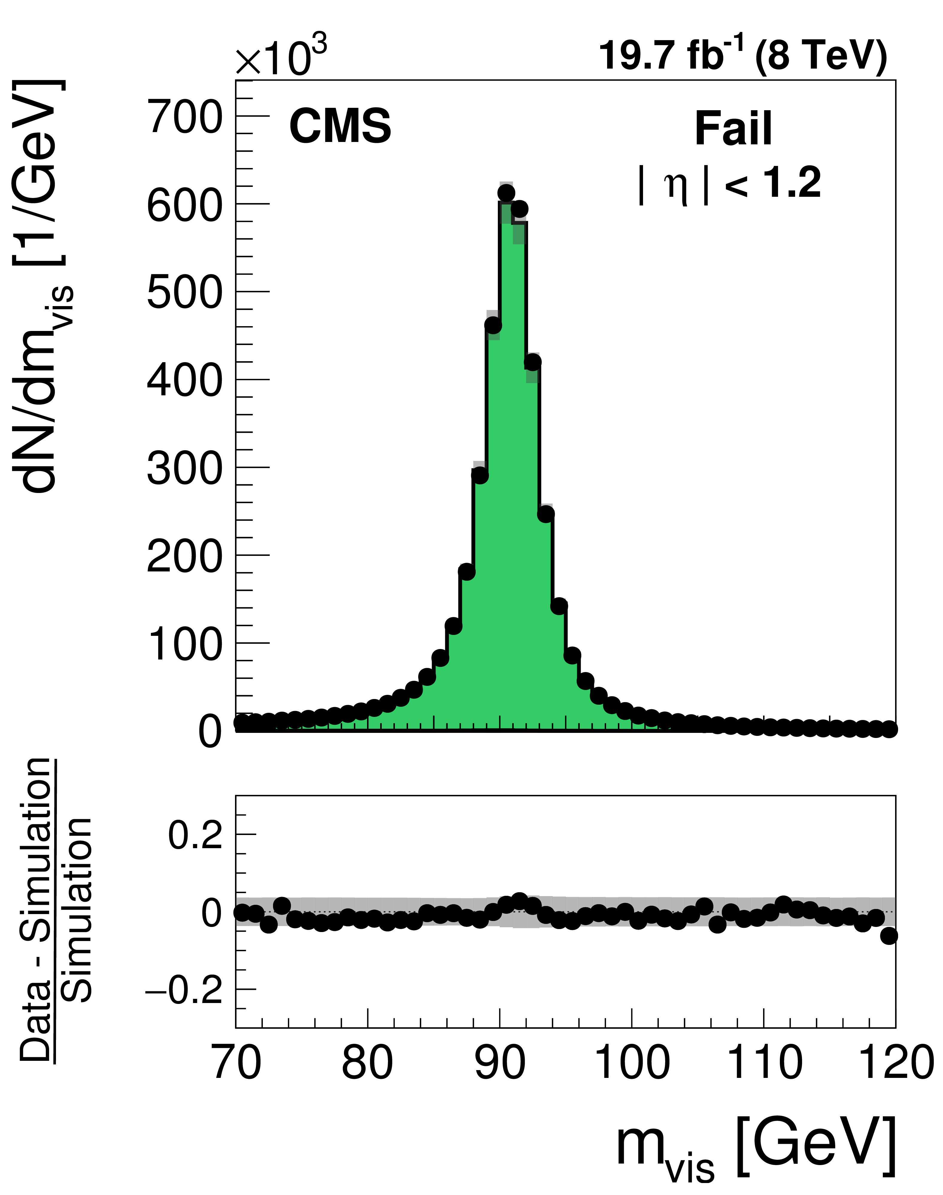
Distribution in the visible mass of the tag and probe pair in the pass (a,d) and fail (b,e) regions, for the loose WP of the electron discriminant in the barrel (a,b) and endcap (d,e) regions. The distributions observed in $ {\mathrm {Z}}/ { {\gamma } ^{*}} \to {\mathrm {e}} {\mathrm {e}}$ candidate events selected in data are compared to the MC expectation, shown for the values of nuisance parameters obtained from the likelihood fit to the data, as described in Section 7.3. The $ {\mathrm {Z}}/ { {\gamma } ^{*}} \to {\ell } {\ell }$ ($ {\ell }= {\mathrm {e}}$, $ {{\mu }}$, $ {\tau }$) events in which either the tag or the probe electron are misidentified are denoted by ``DY others''. The $ {\mathrm {t}} {\overline {\mathrm {t}}}$, single top quark, and diboson backgrounds yield a negligible contribution to the selected event sample and, while present in the fit, are omitted from the legend. The ``Uncertainty'' band represents the statistical and systematic uncertainties added in quadrature. |
png pdf |
Figure 23-b:
Distribution in the visible mass of the tag and probe pair in the pass (a,d) and fail (b,e) regions, for the loose WP of the electron discriminant in the barrel (a,b) and endcap (d,e) regions. The distributions observed in $ {\mathrm {Z}}/ { {\gamma } ^{*}} \to {\mathrm {e}} {\mathrm {e}}$ candidate events selected in data are compared to the MC expectation, shown for the values of nuisance parameters obtained from the likelihood fit to the data, as described in Section 7.3. The $ {\mathrm {Z}}/ { {\gamma } ^{*}} \to {\ell } {\ell }$ ($ {\ell }= {\mathrm {e}}$, $ {{\mu }}$, $ {\tau }$) events in which either the tag or the probe electron are misidentified are denoted by ``DY others''. The $ {\mathrm {t}} {\overline {\mathrm {t}}}$, single top quark, and diboson backgrounds yield a negligible contribution to the selected event sample and, while present in the fit, are omitted from the legend. The ``Uncertainty'' band represents the statistical and systematic uncertainties added in quadrature. |

png pdf |
Figure 23-c:
Distribution in the visible mass of the tag and probe pair in the pass (a,d) and fail (b,e) regions, for the loose WP of the electron discriminant in the barrel (a,b) and endcap (d,e) regions. The distributions observed in $ {\mathrm {Z}}/ { {\gamma } ^{*}} \to {\mathrm {e}} {\mathrm {e}}$ candidate events selected in data are compared to the MC expectation, shown for the values of nuisance parameters obtained from the likelihood fit to the data, as described in Section 7.3. The $ {\mathrm {Z}}/ { {\gamma } ^{*}} \to {\ell } {\ell }$ ($ {\ell }= {\mathrm {e}}$, $ {{\mu }}$, $ {\tau }$) events in which either the tag or the probe electron are misidentified are denoted by ``DY others''. The $ {\mathrm {t}} {\overline {\mathrm {t}}}$, single top quark, and diboson backgrounds yield a negligible contribution to the selected event sample and, while present in the fit, are omitted from the legend. The ``Uncertainty'' band represents the statistical and systematic uncertainties added in quadrature. |
png pdf |
Figure 23-d:
Distribution in the visible mass of the tag and probe pair in the pass (a,d) and fail (b,e) regions, for the loose WP of the electron discriminant in the barrel (a,b) and endcap (d,e) regions. The distributions observed in $ {\mathrm {Z}}/ { {\gamma } ^{*}} \to {\mathrm {e}} {\mathrm {e}}$ candidate events selected in data are compared to the MC expectation, shown for the values of nuisance parameters obtained from the likelihood fit to the data, as described in Section 7.3. The $ {\mathrm {Z}}/ { {\gamma } ^{*}} \to {\ell } {\ell }$ ($ {\ell }= {\mathrm {e}}$, $ {{\mu }}$, $ {\tau }$) events in which either the tag or the probe electron are misidentified are denoted by ``DY others''. The $ {\mathrm {t}} {\overline {\mathrm {t}}}$, single top quark, and diboson backgrounds yield a negligible contribution to the selected event sample and, while present in the fit, are omitted from the legend. The ``Uncertainty'' band represents the statistical and systematic uncertainties added in quadrature. |
png pdf |
Figure 23-e:
Distribution in the visible mass of the tag and probe pair in the pass (a,d) and fail (b,e) regions, for the loose WP of the electron discriminant in the barrel (a,b) and endcap (d,e) regions. The distributions observed in $ {\mathrm {Z}}/ { {\gamma } ^{*}} \to {\mathrm {e}} {\mathrm {e}}$ candidate events selected in data are compared to the MC expectation, shown for the values of nuisance parameters obtained from the likelihood fit to the data, as described in Section 7.3. The $ {\mathrm {Z}}/ { {\gamma } ^{*}} \to {\ell } {\ell }$ ($ {\ell }= {\mathrm {e}}$, $ {{\mu }}$, $ {\tau }$) events in which either the tag or the probe electron are misidentified are denoted by ``DY others''. The $ {\mathrm {t}} {\overline {\mathrm {t}}}$, single top quark, and diboson backgrounds yield a negligible contribution to the selected event sample and, while present in the fit, are omitted from the legend. The ``Uncertainty'' band represents the statistical and systematic uncertainties added in quadrature. |
png pdf |
Figure 23-f:
Distribution in the visible mass of the tag and probe pair in the pass (a,d) and fail (b,e) regions, for the loose WP of the electron discriminant in the barrel (a,b) and endcap (d,e) regions. The distributions observed in $ {\mathrm {Z}}/ { {\gamma } ^{*}} \to {\mathrm {e}} {\mathrm {e}}$ candidate events selected in data are compared to the MC expectation, shown for the values of nuisance parameters obtained from the likelihood fit to the data, as described in Section 7.3. The $ {\mathrm {Z}}/ { {\gamma } ^{*}} \to {\ell } {\ell }$ ($ {\ell }= {\mathrm {e}}$, $ {{\mu }}$, $ {\tau }$) events in which either the tag or the probe electron are misidentified are denoted by ``DY others''. The $ {\mathrm {t}} {\overline {\mathrm {t}}}$, single top quark, and diboson backgrounds yield a negligible contribution to the selected event sample and, while present in the fit, are omitted from the legend. The ``Uncertainty'' band represents the statistical and systematic uncertainties added in quadrature. |
png pdf |
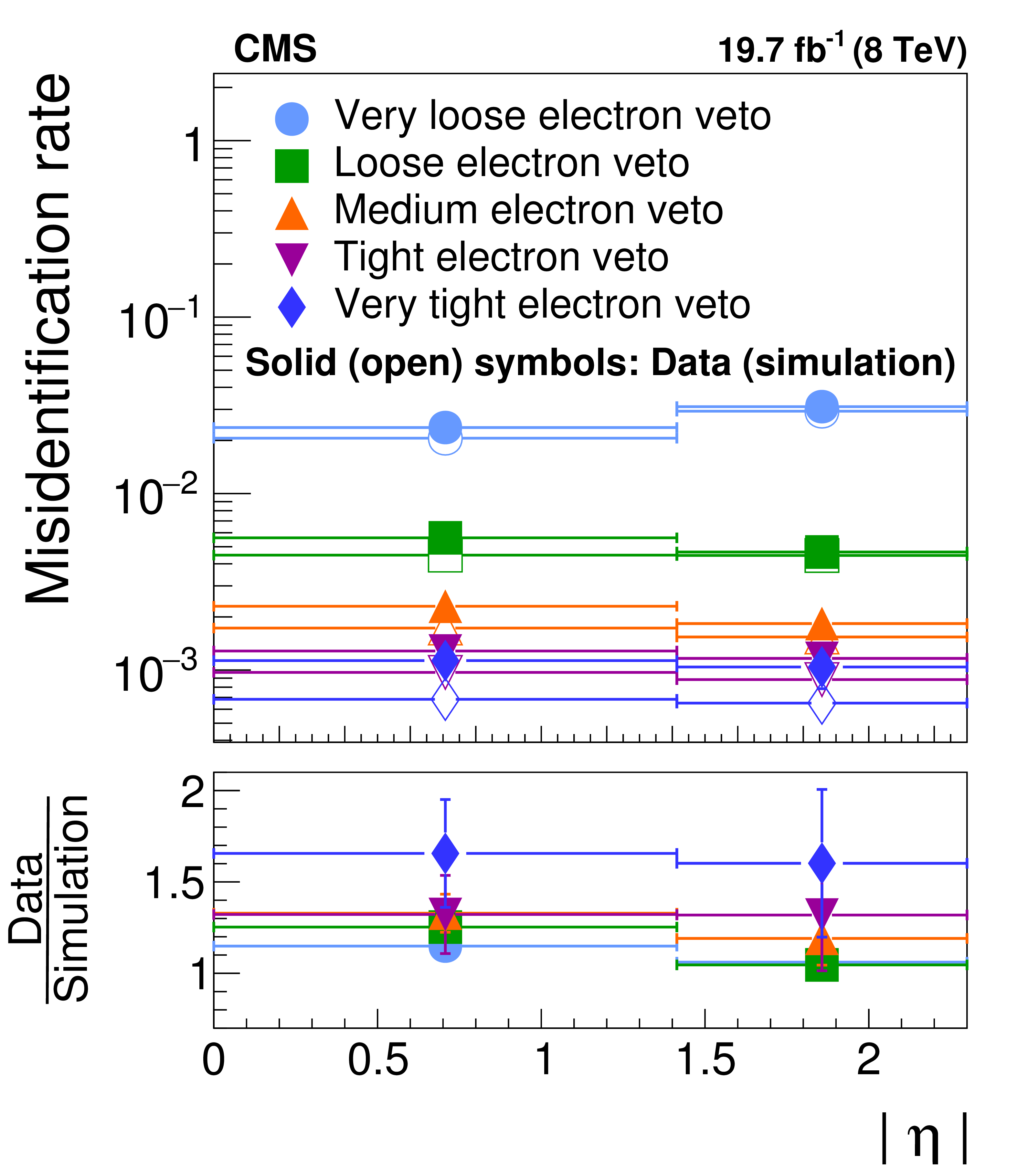
Figure 24:
Probability for electrons in $ {\mathrm {Z}}/ { {\gamma } ^{*}} \to {\mathrm {e}} {\mathrm {e}}$ events to pass different WP of the discriminant against electrons. The $ {\mathrm {e}}\to { {\tau }_{\mathrm {h}}} $ misidentification rates measured in data are compared to the MC expectation, separately for electrons in the barrel ($ {| \eta | } <$ 1.46) and in the endcap ($ {| \eta | } > $ 1.56) regions of the electromagnetic calorimeter. |

png pdf |
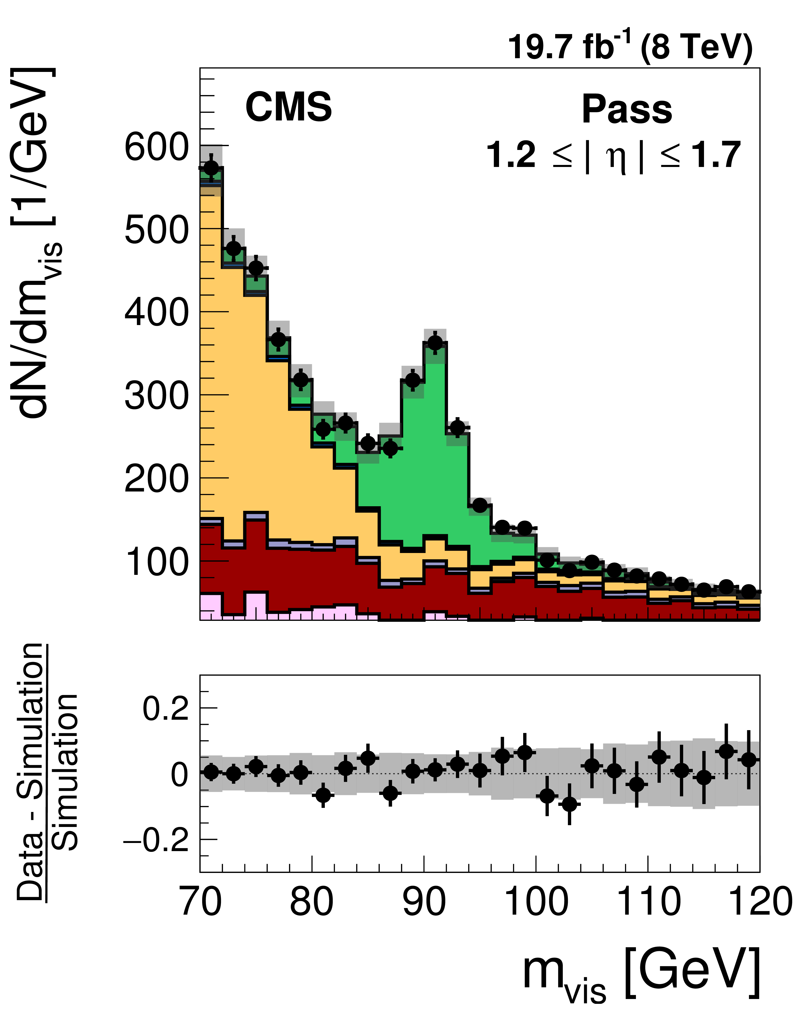
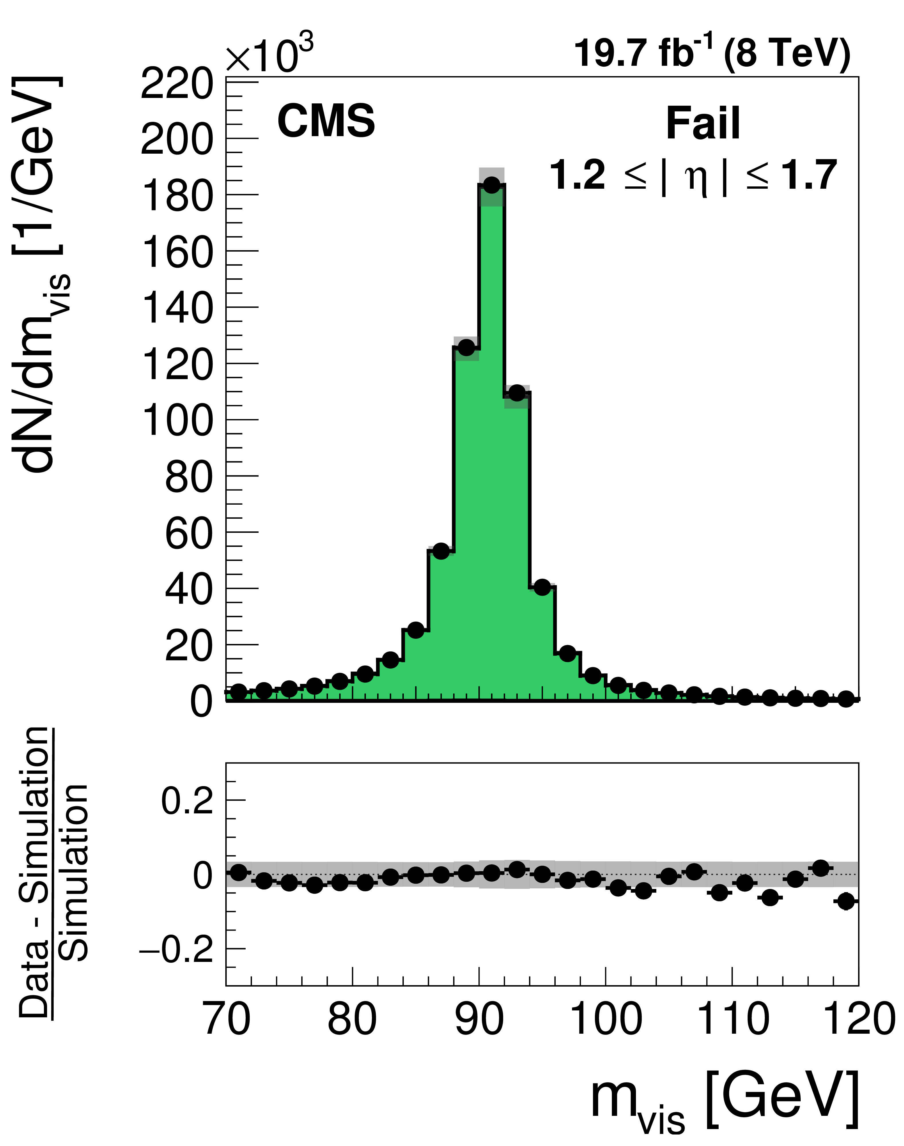
Figure 25-a:
Distribution in the mass of the tag and probe pair in the pass (a,d) and fail (b,e) regions, for the loose WP of the cutoff-based muon discriminant in the region $ {| \eta | } <$ 1.2 (a,b) and 1.2 $\leq {| \eta | } \leq$ 1.7 (d,e). The distributions in $ {\mathrm {Z}}/ { {\gamma } ^{*}} \to {{\mu }} {{\mu }}$ candidate events selected in data are compared to the MC expectation, shown for the values of nuisance parameters obtained from the likelihood fit to the data, as described in Section 7.3. The $ {\mathrm {Z}}/ { {\gamma } ^{*}} \to {\ell } {\ell }$ ($ {\ell }= {\mathrm {e}}$, $ {{\mu }}$, $ {\tau }$) events in which either the tag or the probe muon are misidentified are denoted by ``DY others''. The ``Uncertainty'' band represents the statistical and systematic uncertainties added in quadrature. |
png pdf |
Figure 25-b:
Distribution in the mass of the tag and probe pair in the pass (a,d) and fail (b,e) regions, for the loose WP of the cutoff-based muon discriminant in the region $ {| \eta | } <$ 1.2 (a,b) and 1.2 $\leq {| \eta | } \leq$ 1.7 (d,e). The distributions in $ {\mathrm {Z}}/ { {\gamma } ^{*}} \to {{\mu }} {{\mu }}$ candidate events selected in data are compared to the MC expectation, shown for the values of nuisance parameters obtained from the likelihood fit to the data, as described in Section 7.3. The $ {\mathrm {Z}}/ { {\gamma } ^{*}} \to {\ell } {\ell }$ ($ {\ell }= {\mathrm {e}}$, $ {{\mu }}$, $ {\tau }$) events in which either the tag or the probe muon are misidentified are denoted by ``DY others''. The ``Uncertainty'' band represents the statistical and systematic uncertainties added in quadrature. |

png pdf |
Figure 25-c:
Distribution in the mass of the tag and probe pair in the pass (a,d) and fail (b,e) regions, for the loose WP of the cutoff-based muon discriminant in the region $ {| \eta | } <$ 1.2 (a,b) and 1.2 $\leq {| \eta | } \leq$ 1.7 (d,e). The distributions in $ {\mathrm {Z}}/ { {\gamma } ^{*}} \to {{\mu }} {{\mu }}$ candidate events selected in data are compared to the MC expectation, shown for the values of nuisance parameters obtained from the likelihood fit to the data, as described in Section 7.3. The $ {\mathrm {Z}}/ { {\gamma } ^{*}} \to {\ell } {\ell }$ ($ {\ell }= {\mathrm {e}}$, $ {{\mu }}$, $ {\tau }$) events in which either the tag or the probe muon are misidentified are denoted by ``DY others''. The ``Uncertainty'' band represents the statistical and systematic uncertainties added in quadrature. |
png pdf |
Figure 25-d:
Distribution in the mass of the tag and probe pair in the pass (a,d) and fail (b,e) regions, for the loose WP of the cutoff-based muon discriminant in the region $ {| \eta | } <$ 1.2 (a,b) and 1.2 $\leq {| \eta | } \leq$ 1.7 (d,e). The distributions in $ {\mathrm {Z}}/ { {\gamma } ^{*}} \to {{\mu }} {{\mu }}$ candidate events selected in data are compared to the MC expectation, shown for the values of nuisance parameters obtained from the likelihood fit to the data, as described in Section 7.3. The $ {\mathrm {Z}}/ { {\gamma } ^{*}} \to {\ell } {\ell }$ ($ {\ell }= {\mathrm {e}}$, $ {{\mu }}$, $ {\tau }$) events in which either the tag or the probe muon are misidentified are denoted by ``DY others''. The ``Uncertainty'' band represents the statistical and systematic uncertainties added in quadrature. |
png pdf |
Figure 25-e:
Distribution in the mass of the tag and probe pair in the pass (a,d) and fail (b,e) regions, for the loose WP of the cutoff-based muon discriminant in the region $ {| \eta | } <$ 1.2 (a,b) and 1.2 $\leq {| \eta | } \leq$ 1.7 (d,e). The distributions in $ {\mathrm {Z}}/ { {\gamma } ^{*}} \to {{\mu }} {{\mu }}$ candidate events selected in data are compared to the MC expectation, shown for the values of nuisance parameters obtained from the likelihood fit to the data, as described in Section 7.3. The $ {\mathrm {Z}}/ { {\gamma } ^{*}} \to {\ell } {\ell }$ ($ {\ell }= {\mathrm {e}}$, $ {{\mu }}$, $ {\tau }$) events in which either the tag or the probe muon are misidentified are denoted by ``DY others''. The ``Uncertainty'' band represents the statistical and systematic uncertainties added in quadrature. |
png pdf |
Figure 25-f:
Distribution in the mass of the tag and probe pair in the pass (a,d) and fail (b,e) regions, for the loose WP of the cutoff-based muon discriminant in the region $ {| \eta | } <$ 1.2 (a,b) and 1.2 $\leq {| \eta | } \leq$ 1.7 (d,e). The distributions in $ {\mathrm {Z}}/ { {\gamma } ^{*}} \to {{\mu }} {{\mu }}$ candidate events selected in data are compared to the MC expectation, shown for the values of nuisance parameters obtained from the likelihood fit to the data, as described in Section 7.3. The $ {\mathrm {Z}}/ { {\gamma } ^{*}} \to {\ell } {\ell }$ ($ {\ell }= {\mathrm {e}}$, $ {{\mu }}$, $ {\tau }$) events in which either the tag or the probe muon are misidentified are denoted by ``DY others''. The ``Uncertainty'' band represents the statistical and systematic uncertainties added in quadrature. |
png pdf |
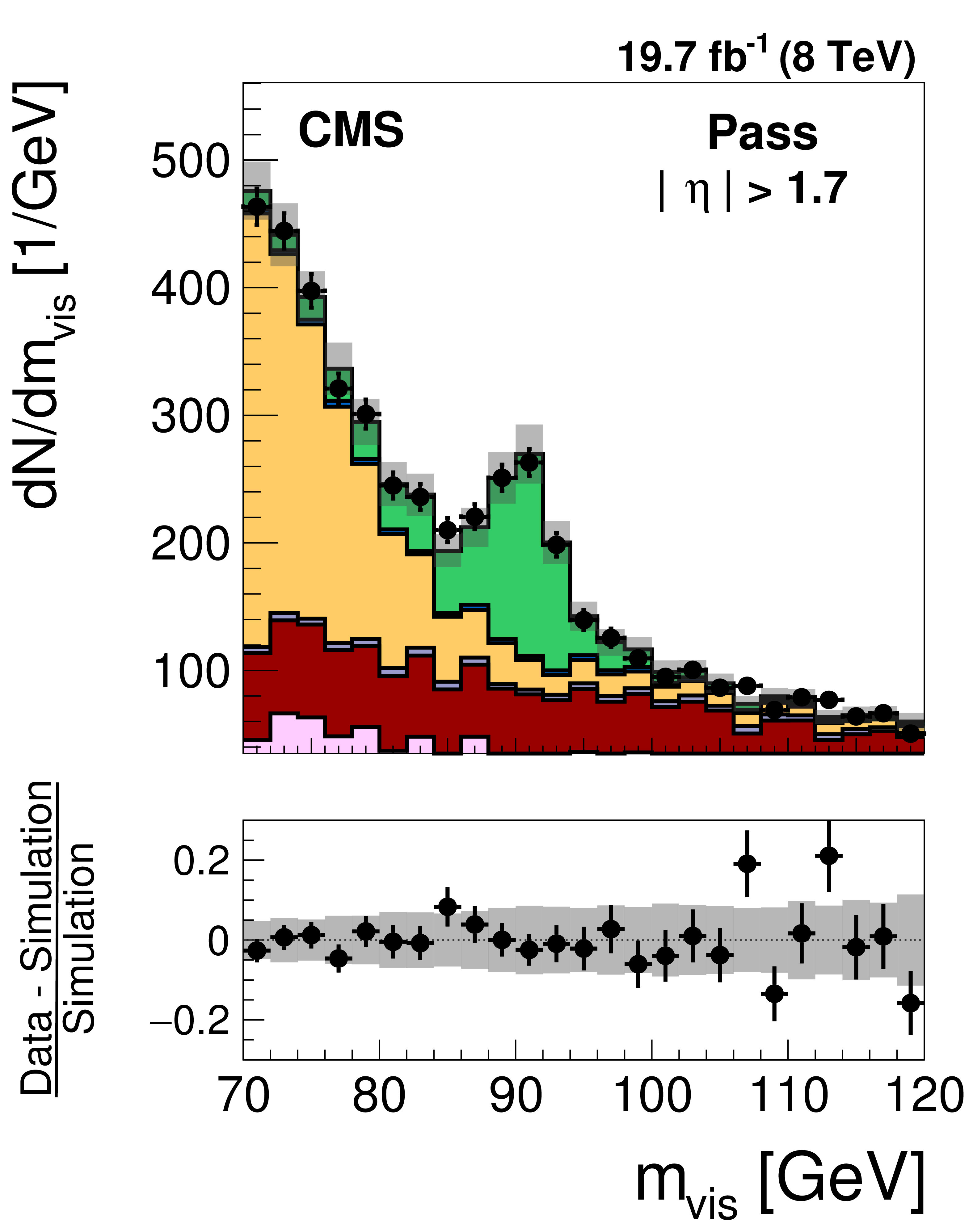
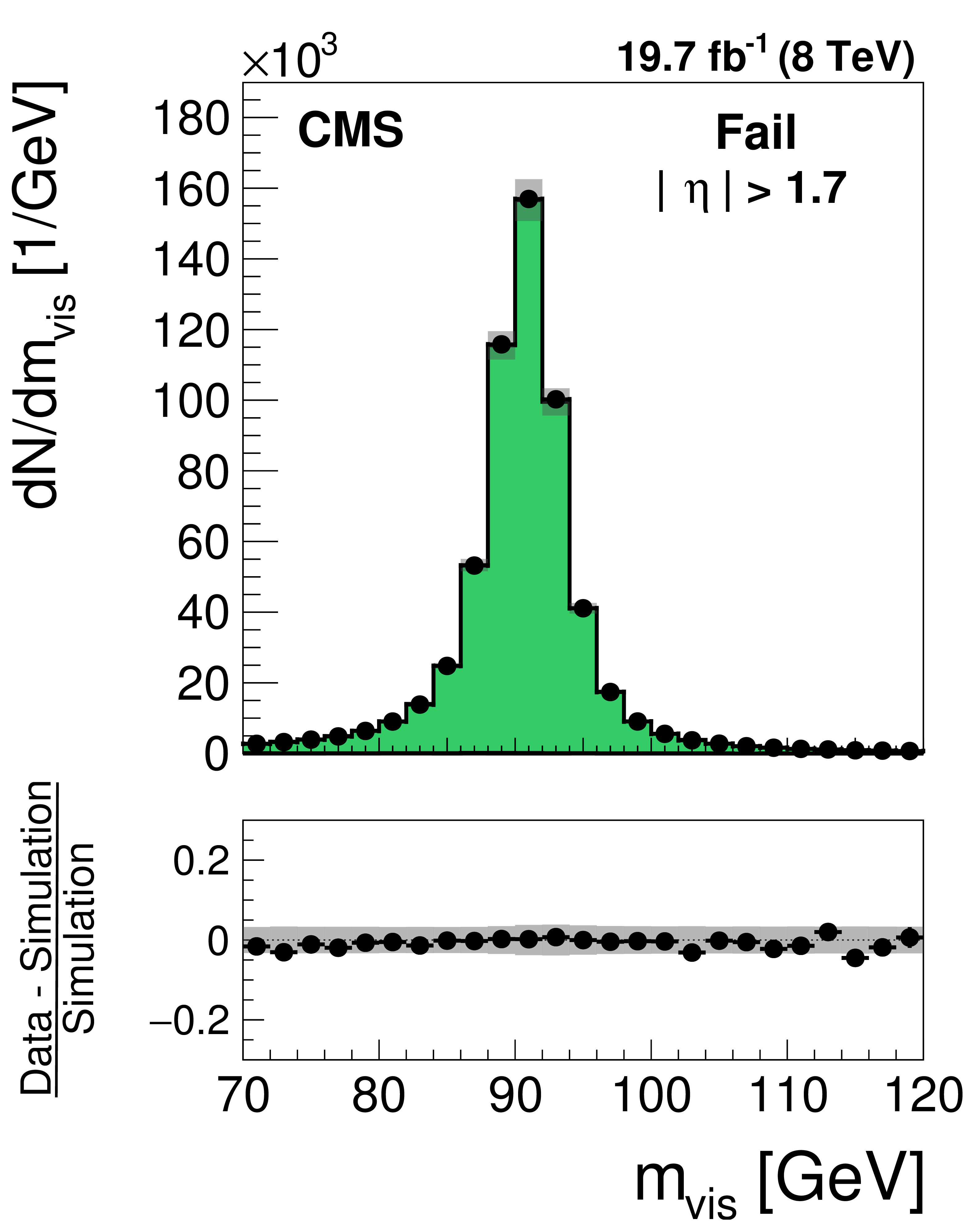
Figure 26-a:
Distribution in the mass of the tag and probe pair in the pass (a) and fail (b) regions, for the loose WP of the cutoff-based muon discriminant in the region $ {| \eta | } > $ 1.7. The distributions in $ {\mathrm {Z}}/ { {\gamma } ^{*}} \to {{\mu }} {{\mu }}$ candidate events selected in data are compared to the MC expectation, shown for the values of nuisance parameters obtained from the likelihood fit to the data, as described in Section 7.3. The $ {\mathrm {Z}}/ { {\gamma } ^{*}} \to {\ell } {\ell }$ ($ {\ell }= {\mathrm {e}}$, $ {{\mu }}$, $ {\tau }$) events in which either the tag or the probe muon are misidentified are denoted by ``DY others''. The ``Uncertainty'' band represents the statistical and systematic uncertainties added in quadrature. |
png pdf |
Figure 26-b:
Distribution in the mass of the tag and probe pair in the pass (a) and fail (b) regions, for the loose WP of the cutoff-based muon discriminant in the region $ {| \eta | } > $ 1.7. The distributions in $ {\mathrm {Z}}/ { {\gamma } ^{*}} \to {{\mu }} {{\mu }}$ candidate events selected in data are compared to the MC expectation, shown for the values of nuisance parameters obtained from the likelihood fit to the data, as described in Section 7.3. The $ {\mathrm {Z}}/ { {\gamma } ^{*}} \to {\ell } {\ell }$ ($ {\ell }= {\mathrm {e}}$, $ {{\mu }}$, $ {\tau }$) events in which either the tag or the probe muon are misidentified are denoted by ``DY others''. The ``Uncertainty'' band represents the statistical and systematic uncertainties added in quadrature. |

png pdf |
Figure 26-c:
Distribution in the mass of the tag and probe pair in the pass (a) and fail (b) regions, for the loose WP of the cutoff-based muon discriminant in the region $ {| \eta | } > $ 1.7. The distributions in $ {\mathrm {Z}}/ { {\gamma } ^{*}} \to {{\mu }} {{\mu }}$ candidate events selected in data are compared to the MC expectation, shown for the values of nuisance parameters obtained from the likelihood fit to the data, as described in Section 7.3. The $ {\mathrm {Z}}/ { {\gamma } ^{*}} \to {\ell } {\ell }$ ($ {\ell }= {\mathrm {e}}$, $ {{\mu }}$, $ {\tau }$) events in which either the tag or the probe muon are misidentified are denoted by ``DY others''. The ``Uncertainty'' band represents the statistical and systematic uncertainties added in quadrature. |
png pdf |
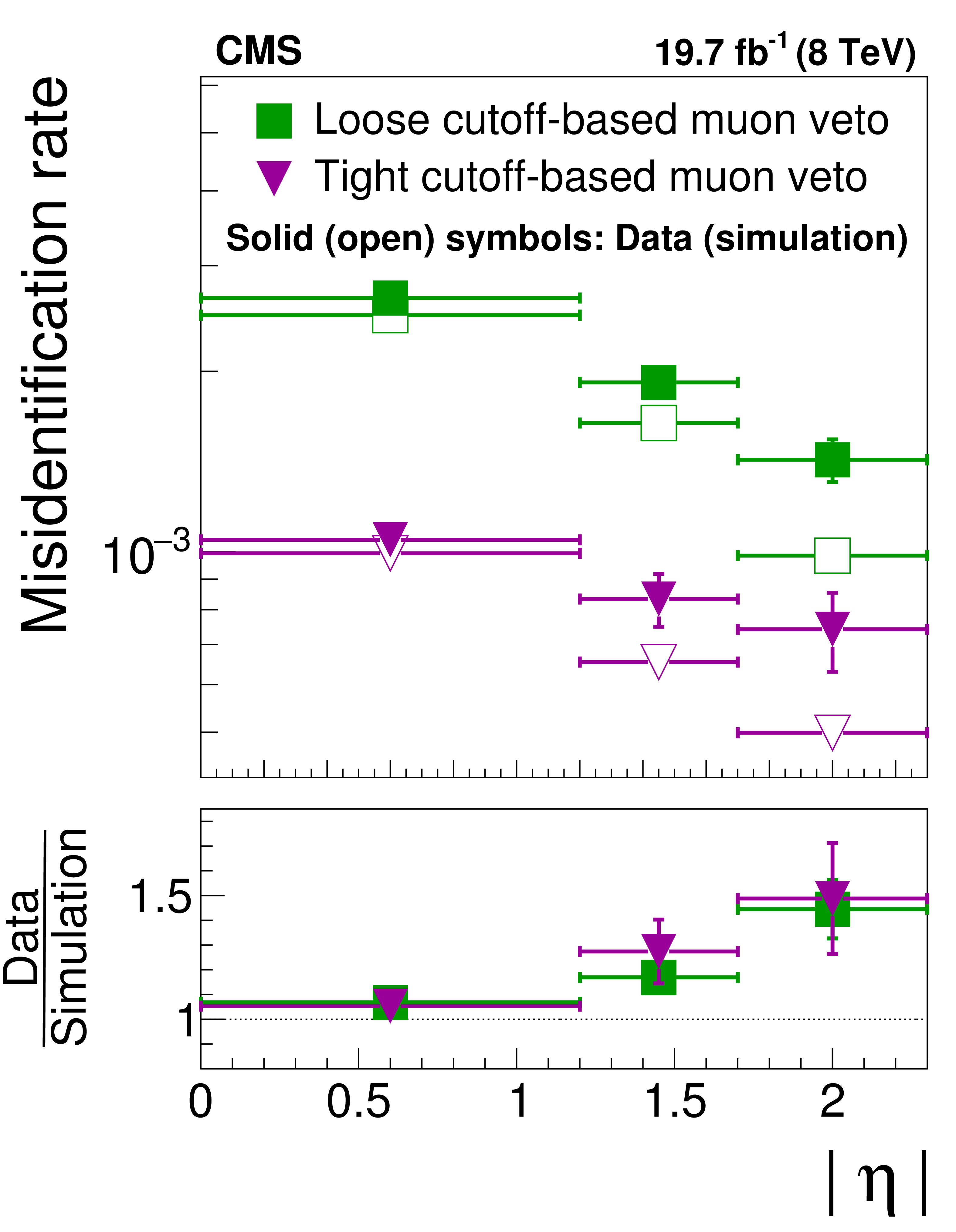
Figure 27-a:
Probability for muons in $ {\mathrm {Z}}/ { {\gamma } ^{*}} \to {{\mu }} {{\mu }}$ events to pass different WP of the (a) cut-based and (b) MVA-based discriminants against muons. The $ {{\mu }}\to { {\tau }_{\mathrm {h}}} $ misidentification rates measured in data are compared to the MC simulation in the regions $ {| \eta | } < $1.2, 1.2 $\leq {| \eta | } \leq $ 1.7, and $ {| \eta | } > $ 1.7. |
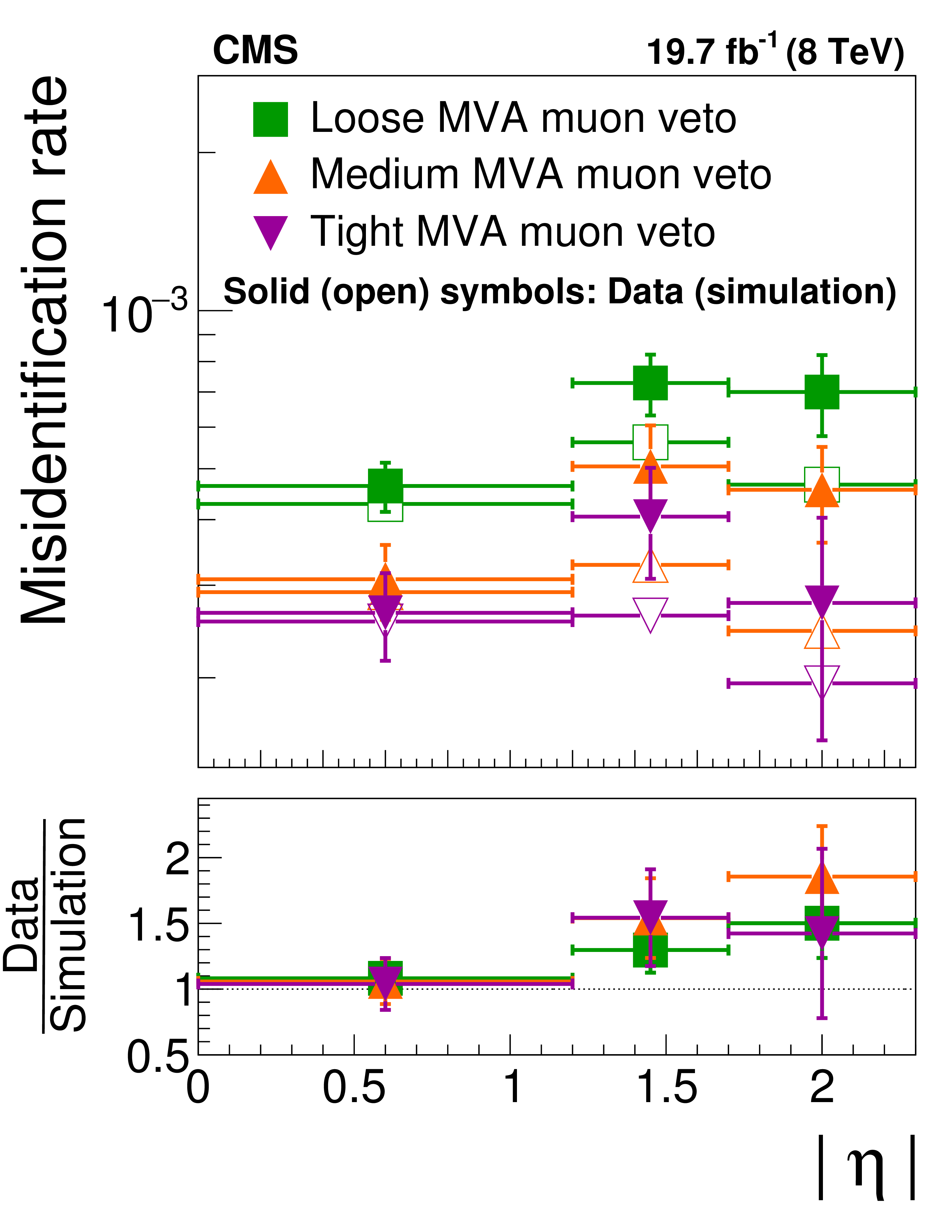
png pdf |
Figure 27-b:
Probability for muons in $ {\mathrm {Z}}/ { {\gamma } ^{*}} \to {{\mu }} {{\mu }}$ events to pass different WP of the (a) cut-based and (b) MVA-based discriminants against muons. The $ {{\mu }}\to { {\tau }_{\mathrm {h}}} $ misidentification rates measured in data are compared to the MC simulation in the regions $ {| \eta | } < $1.2, 1.2 $\leq {| \eta | } \leq $ 1.7, and $ {| \eta | } > $ 1.7. |
| Tables | |
png pdf |
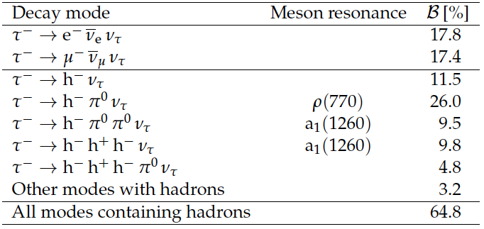
Table 1:
Approximate branching fractions ($\mathcal {B}$) of different $ {\tau }$ decay modes [18]. The generic symbol $\mathrm {h}^{-}$ represents a charged hadron (either a pion or a kaon). Charge conjugation invariance is assumed in this paper. |
png pdf |
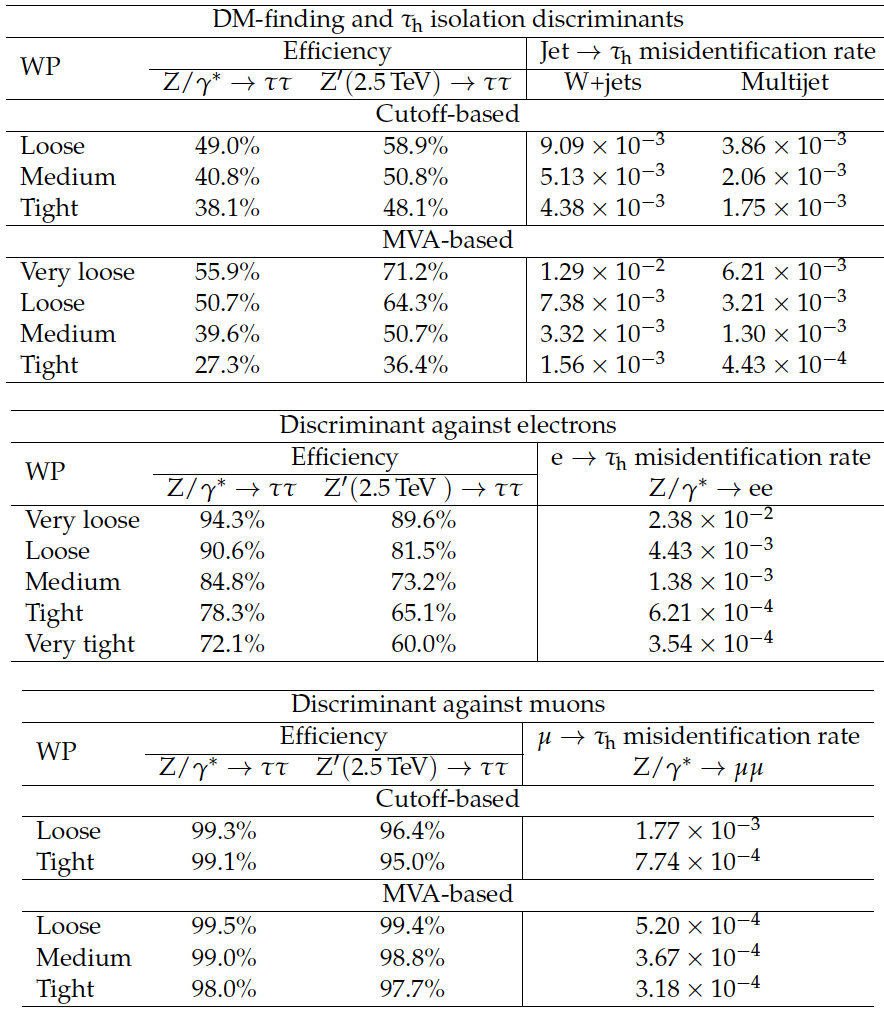
Table 2:
Expected efficiencies and misidentification rates of various $ { {\tau }_{\mathrm {h}}} $ identification discriminants, averaged over $ {p_{\mathrm {T}}} $ and $\eta $, for pileup conditions characteristic of the LHC Run 1 data-taking period. The DM-finding criterion refers to the requirement that the $ { {\tau }_{\mathrm {h}}} $ candidate be reconstructed in one of the decay modes $ {\mathrm {h}^{\pm }} $, $ {\mathrm {h}^{\pm } { {\pi ^0}}} $, $ {\mathrm {h}^{\pm } { {\pi ^0}} { {\pi ^0}}} $, or $ {\mathrm {h}^{\pm }\mathrm {h}^{\mp }\mathrm {h}^{\pm }} $ (cf. Section 5.1). |
png pdf |
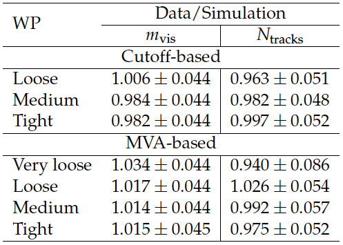
Table 3:
Data-to-MC ratios of the efficiency for $ { {\tau }_{\mathrm {h}}} $ decays to pass different identification discriminants, measured in $ {\mathrm {Z}}/ { {\gamma } ^{*}} \to {\tau } {\tau }\to {{\mu }} { {\tau }_{\mathrm {h}}} $ events. The results obtained using the observables $ {m_{\text {vis}}} $ and $ {N_{\text {tracks}}} $ are quoted in separate columns. |
png pdf |
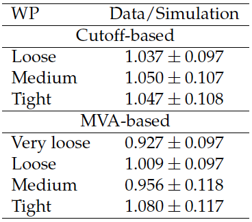
Table 4:
Data-to-MC ratios of the efficiency for $ { {\tau }_{\mathrm {h}}} $ decays in $ {\mathrm {t}} {\overline {\mathrm {t}}}\to {\mathrm {b}} {\overline {\mathrm {b}}} {{\mu }} { {\tau }_{\mathrm {h}}} $ events to pass different $ { {\tau }_{\mathrm {h}}} $ identification discriminants. |
png pdf |
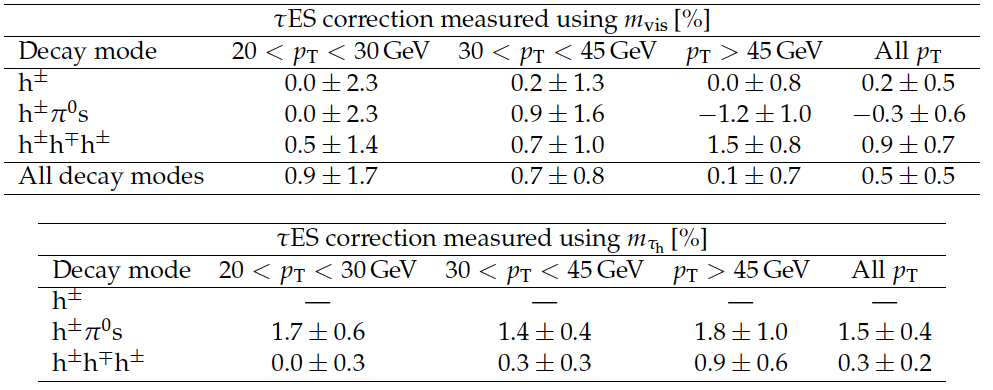
Table 5:
Energy scale corrections for $ { {\tau }_{\mathrm {h}}} $ measured in $ {\mathrm {Z}}/ { {\gamma } ^{*}} \to {\tau } {\tau }$ events, using the distribution in $ {m_{\text {vis}}} $ and $m_{ { {\tau }_{\mathrm {h}}} }$, for $ { {\tau }_{\mathrm {h}}} $ reconstructed in different decay modes and $ { {\tau }_{\mathrm {h}}} $ $ {p_{\mathrm {T}}} $ bins. The $ {\tau }$ES corrections measured for the combination of all $ { {\tau }_{\mathrm {h}}} $ decay modes and $ {p_{\mathrm {T}}} $ bins are also given in the table. It is obtained by means of an independent fit and hence may be different from the average of $ {\tau }$ES corrections measured for individual decay modes. |

png pdf |
Table 6:
Probability for electrons to pass different WP of the discriminant against electrons. The $ {\mathrm {e}}\to { {\tau }_{\mathrm {h}}} $ misidentification rates measured in $ {\mathrm {Z}}/ { {\gamma } ^{*}} \to {\mathrm {e}} {\mathrm {e}}$ events are compared to the MC expectation, separately for electrons in the ECAL barrel and endcap regions. |
png pdf |
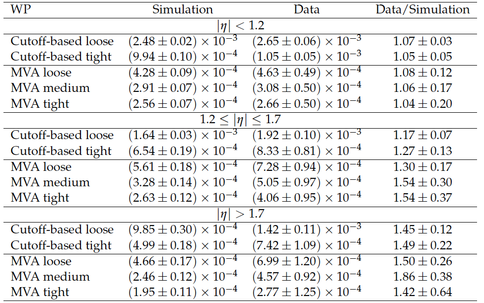
Table 7:
Probability for muons to pass different WP of the cutoff-based and MVA-based discriminants against muons. The $ {{\mu }}\to { {\tau }_{\mathrm {h}}} $ misidentification rates measured in $ {\mathrm {Z}}/ { {\gamma } ^{*}} \to {{\mu }} {{\mu }}$ events are compared to the MC predictions in the regions $ {| \eta | } < $ 1.2, 1.2 $\leq {| \eta | } \leq $ 1.7, and $ {| \eta | } >$ 1.7. |
| Summary |
|
The algorithms used by the CMS experiment for reconstruction and identification of hadronic $\tau$ decays in Run 1 data from the LHC have been presented, and their performance validated with proton-proton collision data recorded at $\sqrt{s} =$ 8 TeV, corresponding to an integrated luminosity of 19.7 fb$^{-1}$. The algorithms achieve a $\tau_{\mathrm{h}}$ identification efficiency of typically 50-60%, and misidentification rates for quark and gluon jets, electrons, and muons that vary between the per mille and per cent level. The reconstruction of different $\tau_{\mathrm{h}}$ decay modes and their energies is demonstrated to be robust against pileup. The $\tau_{\mathrm{h}}$ identification efficiency measured in the data agrees with the MC expectation within the uncertainty of the measurement of about 4.5%. The measured $\text{jet} \to\tau_{\mathrm{h}}$ misidentification rates are about 20% higher than predicted for low-pT jets and 20% lower for high-pT jets. The probabilities for electrons and muons to pass the $\tau_{\mathrm{h}}$ identification criteria, including dedicated discriminants that were developed to reduce the $\mathrm{e} \to \tau_{\mathrm{h}}$ and $\mu \to \tau_{\mathrm{h}}$ misidentification rates, have been measured with a precision that ranges from a few % and 25%, for loose and tight working points, respectively. The measured misidentification rate for electrons exceeds the MC expectation by up to a factor 1.7. The differences observed between data and MC simulation in the probabilities for jets, electrons, and muons to be misidentified as $\tau_{\mathrm{h}}$ decays have been taken into account in physics analyses by applying appropriate MC-to-data correction factors. The procedures developed for studying $\tau_{\mathrm{h}}$ decays have provided a powerful tool for precision measurements as well as for the search for new phenomena beyond the standard model in Run 2 of the LHC. |
|
|
Compact Muon Solenoid LHC, CERN |
|

|

|

|

|

|