

Compact Muon Solenoid
LHC, CERN
| CMS-TRK-11-001 ; CERN-PH-EP-2014-070 | ||
| Description and performance of track and primary-vertex reconstruction with the CMS tracker | ||
| CMS Collaboration | ||
| 26 May 2014 | ||
| J. Instrum. 9 (2014) P10009 | ||
| Abstract: A description is provided of the software algorithms developed for the CMS tracker both for reconstructing charged-particle trajectories in proton-proton interactions and for using the resulting tracks to estimate the positions of the LHC luminous region and individual primary-interaction vertices. Despite the very hostile environment at the LHC, the performance obtained with these algorithms is found to be excellent. For $ \mathrm{ t\bar{t} } $ events under typical 2011 pileup conditions, the average track-reconstruction efficiency for promptly-produced charged particles with transverse momenta of $p_{ \mathrm{T} }$ > 0.9 GeV is 94% for pseudorapidities of |$\eta$| < 0.9 and 85% for |$\eta$| between 0.9 and 2.5. The inefficiency is caused mainly by hadrons that undergo nuclear interactions in the tracker material. For isolated muons, the corresponding efficiencies are essentially 100%. For isolated muons of $p_{ \mathrm{T} }$ = 100 GeV emitted at |$\eta$| lower than 1.4, the resolutions are approximately 2.8% in $p_{ \mathrm{T} }$, and respectively, 10 microns and 30 microns in the transverse and longitudinal impact parameters. The position resolution achieved for reconstructed primary vertices that correspond to interesting pp collisions is 10-12 microns in each of the three spatial dimensions. The tracking and vertexing software is fast and flexible, and easily adaptable to other functions, such as fast tracking for the trigger, or dedicated tracking for electrons that takes into account bremsstrahlung. | ||
| Links: e-print arXiv:1405.6569 [physics.ins-det] (PDF) ; CDS record ; inSPIRE record ; CADI line (restricted) ; | ||
| Figures | |

png pdf |
Figure 1:
Schematic cross section through the CMS tracker in the $r$-$z$ plane. In this view, the tracker is symmetric about the horizontal line $r=0$, so only the top half is shown here. The centre of the tracker, corresponding to the approximate position of the pp collision point, is indicated by a star. Green dashed lines help the reader understand which modules belong to each of the named tracker subsystems. Strip tracker modules that provide 2-D hits are shown by thin, black lines, while those permitting the reconstruction of hit positions in 3-D are shown by thick, blue lines. The latter actually each consist of two back-to-back strip modules, in which one module is rotated through a `stereo' angle. The pixel modules, shown by the red lines, also provide 3-D hits. Within a given layer, each module is shifted slightly in $r$ or $z$ with respect to its neighbouring modules, which allows them to overlap, thereby avoiding gaps in the acceptance. |
png pdf |
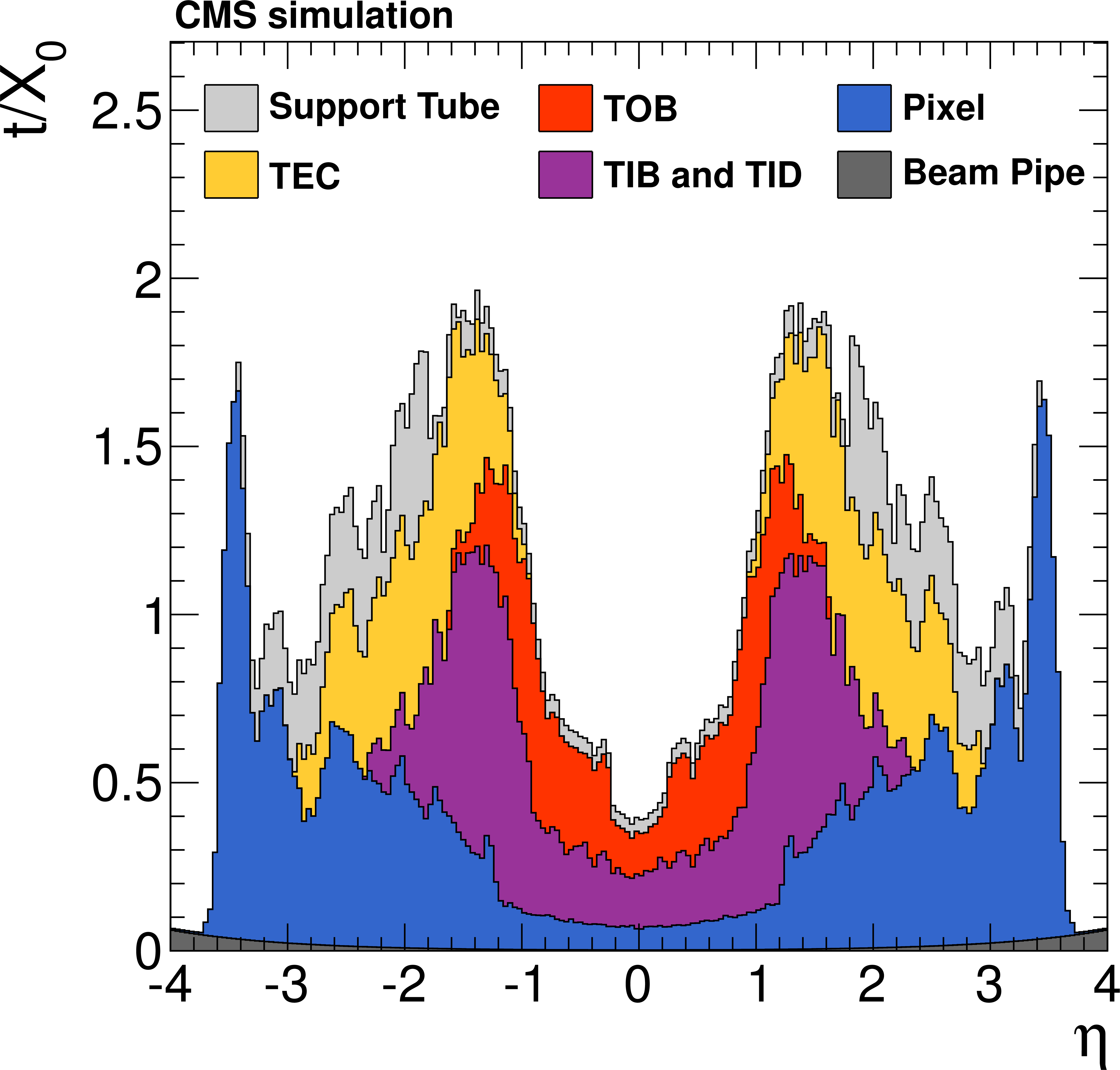
Figure 2-a:
Total thickness $t$ of the tracker material traversed by a particle produced at the nominal interaction point, as a function of pseudorapidity $\eta $, expressed in units of radiation length $X_0$ (a) and nuclear interaction length $\lambda _I$ (b). The contribution to the total material budget of each of the subsystems that comprise the CMS tracker is shown, together with contributions from the beam pipe and from the support tube that surrounds the tracker. |

png pdf |
Figure 2-b:
Total thickness $t$ of the tracker material traversed by a particle produced at the nominal interaction point, as a function of pseudorapidity $\eta $, expressed in units of radiation length $X_0$ (a) and nuclear interaction length $\lambda _I$ (b). The contribution to the total material budget of each of the subsystems that comprise the CMS tracker is shown, together with contributions from the beam pipe and from the support tube that surrounds the tracker. |
png pdf |
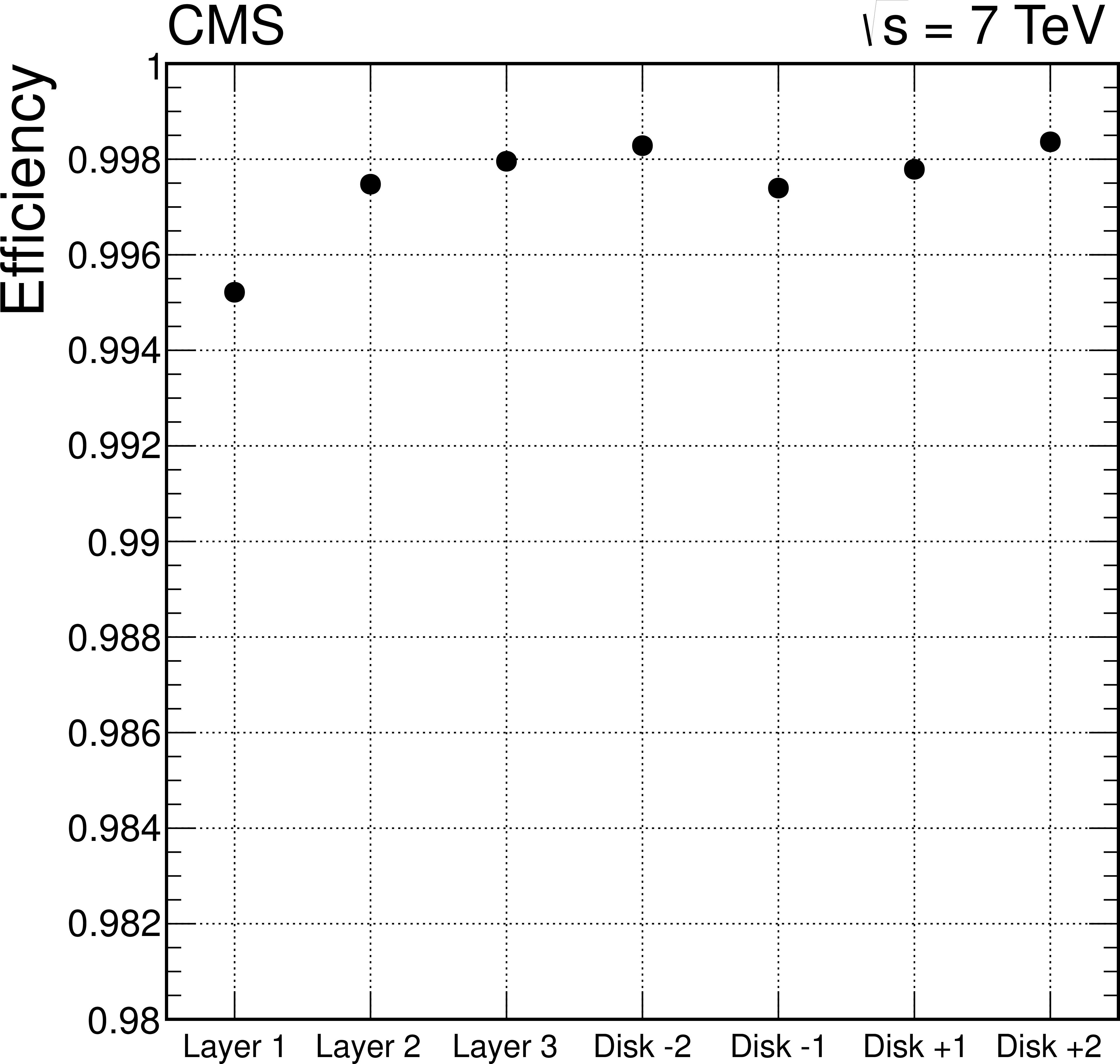
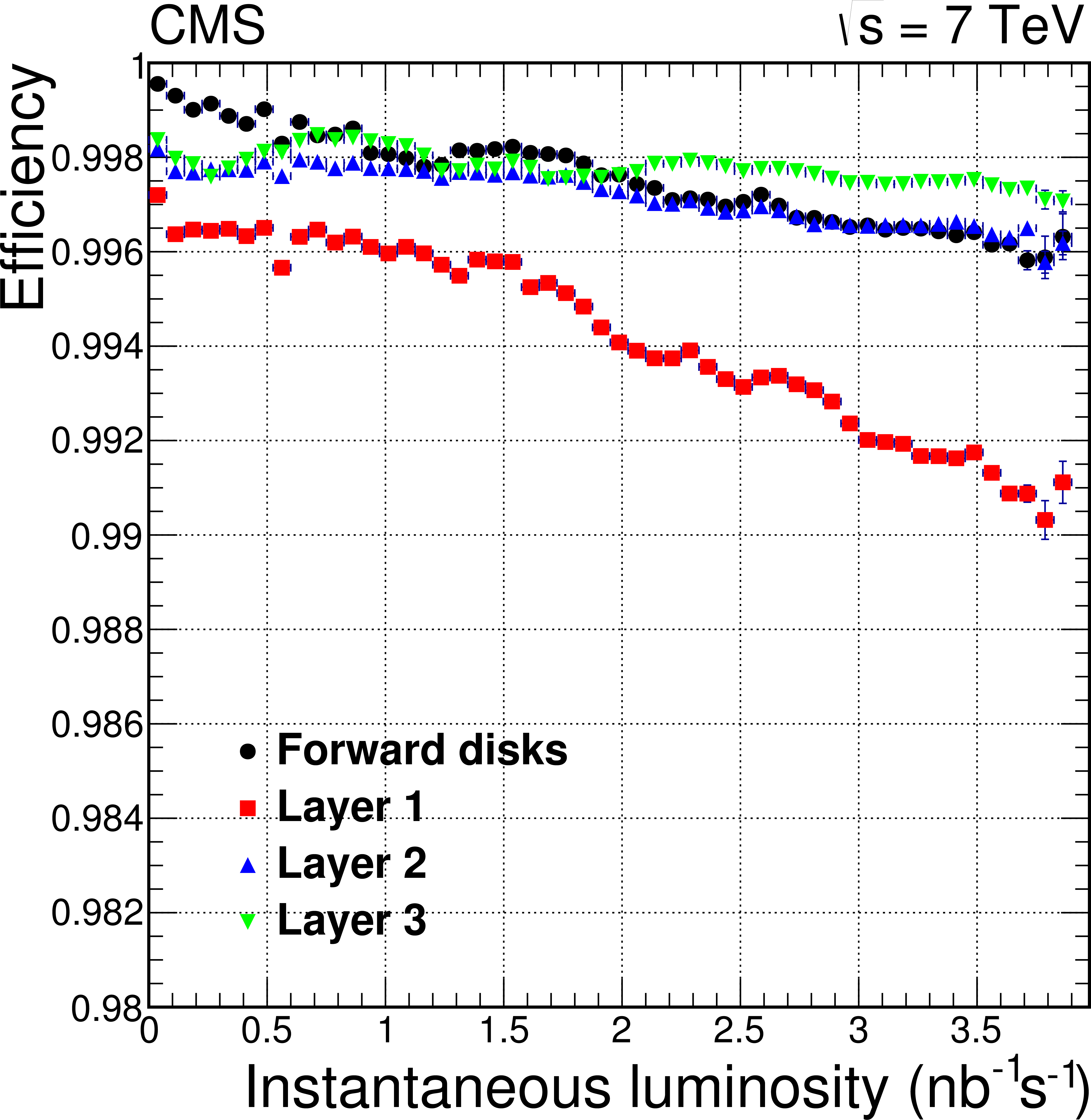
Figure 3-a:
The average hit efficiency for layers or disks in the pixel detector excluding defective modules (a), and the average hit efficiency as a function of instantaneous luminosity (b). The peak luminosity ranged from 1 to 4 nb$^{-1}$s$^{-1}$ during the data taking. |
png pdf |
Figure 3-b:
The average hit efficiency for layers or disks in the pixel detector excluding defective modules (a), and the average hit efficiency as a function of instantaneous luminosity (b). The peak luminosity ranged from 1 to 4 nb$^{-1}$s$^{-1}$ during the data taking. |
png pdf |
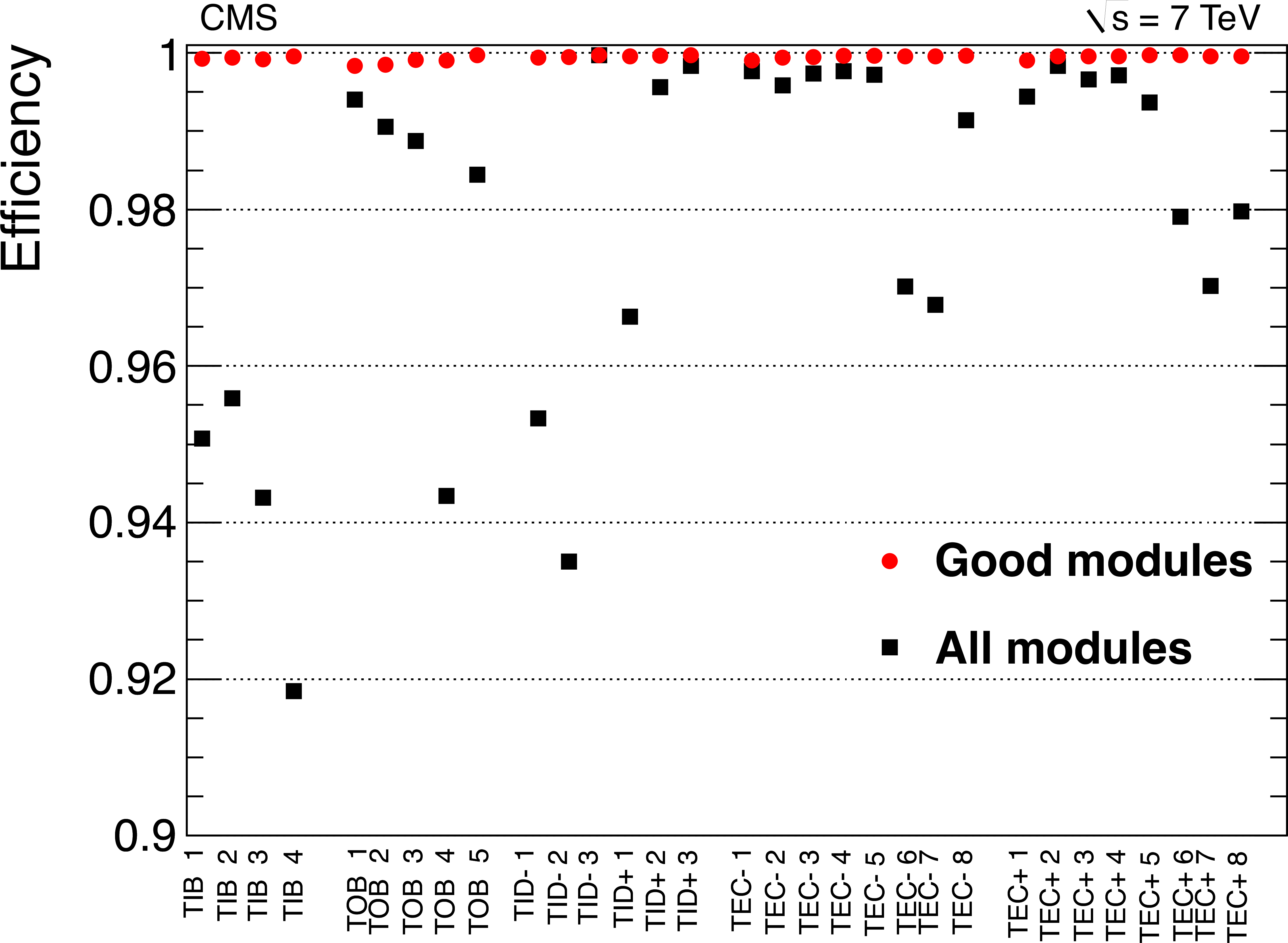
Figure 4:
Average hit efficiency for layers or disks in the strip tracker. The black squares show the hit efficiency in all modules, and the red dots for modules included in the readout. |
png pdf |
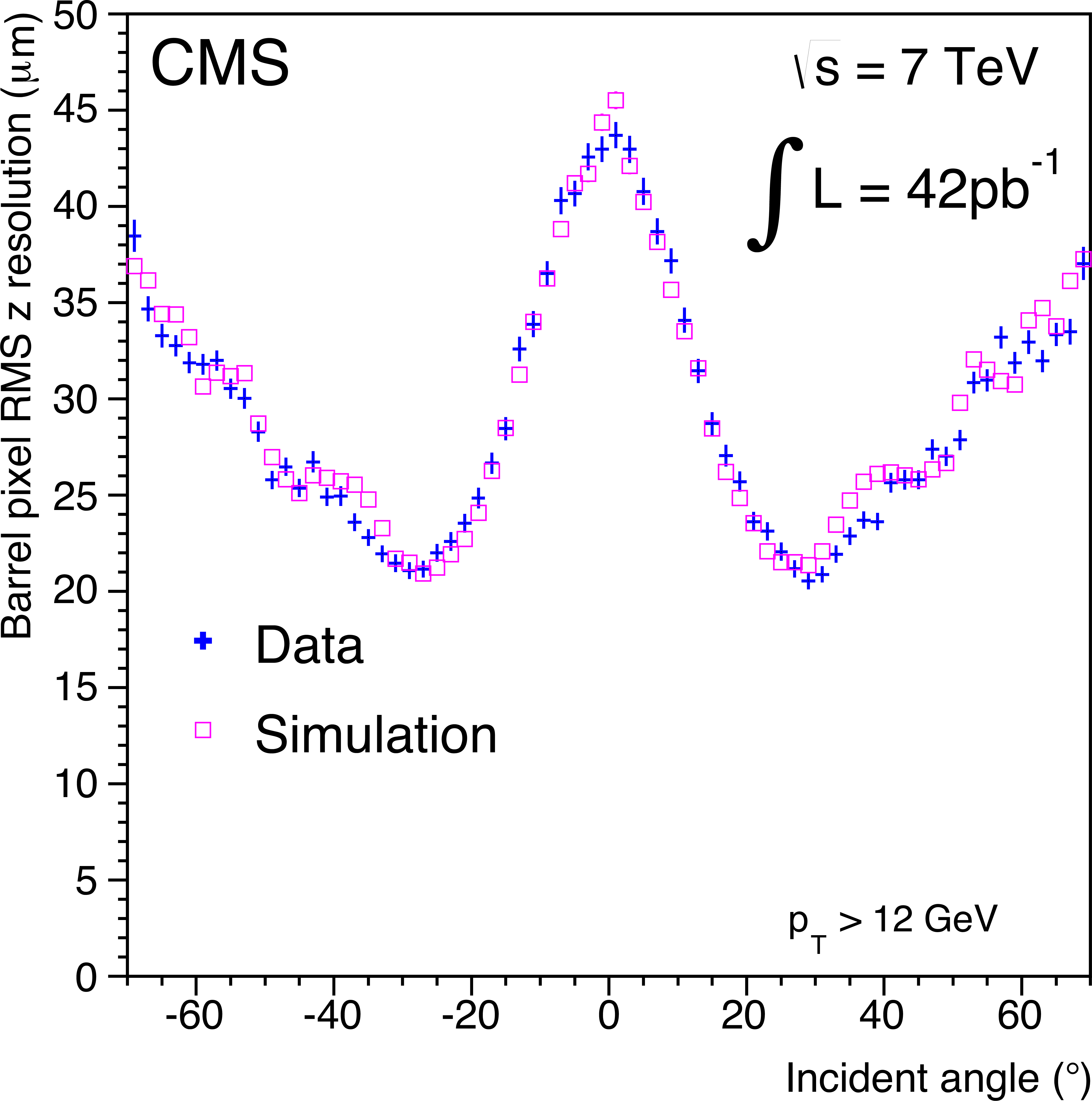
Figure 5:
Resolution in the longitudinal ($z$) coordinate of hits in the barrel section of the pixel detector, shown as a function of the incident angle of the track, which is defined as $90^\circ -\theta $, and equals the angle of the track relative to the normal to the plane of the sensor. Data are compared with MC simulation for tracks with $ {p_{\mathrm {T}}} >$ 12 GeV. |
png pdf |
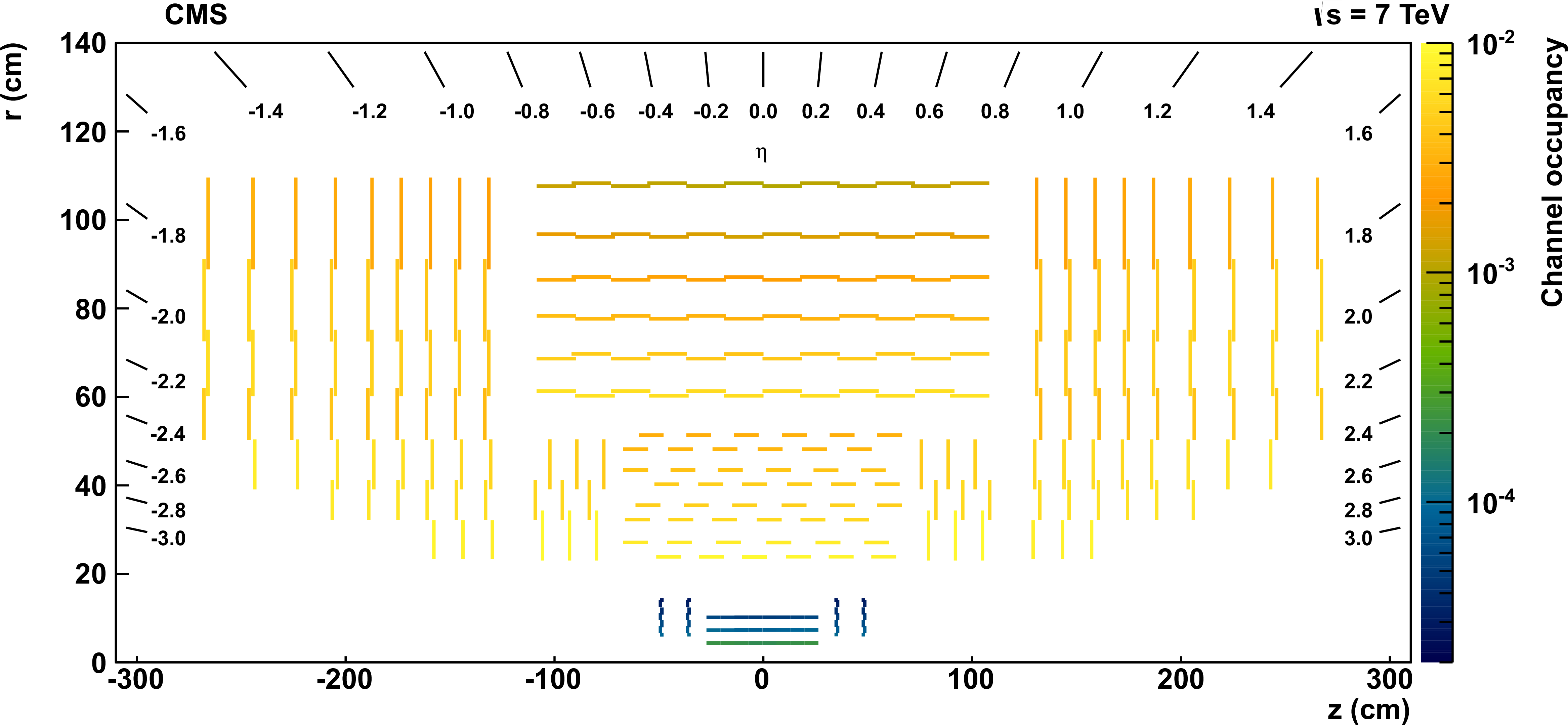
Figure 6:
Channel occupancy (labelled by the scale on the right) for CMS silicon detectors in events taken with unbiased triggers with an average of nine pp interactions per beam crossing, displayed as a function of $\eta $, $r$, and $z$. |
png pdf |
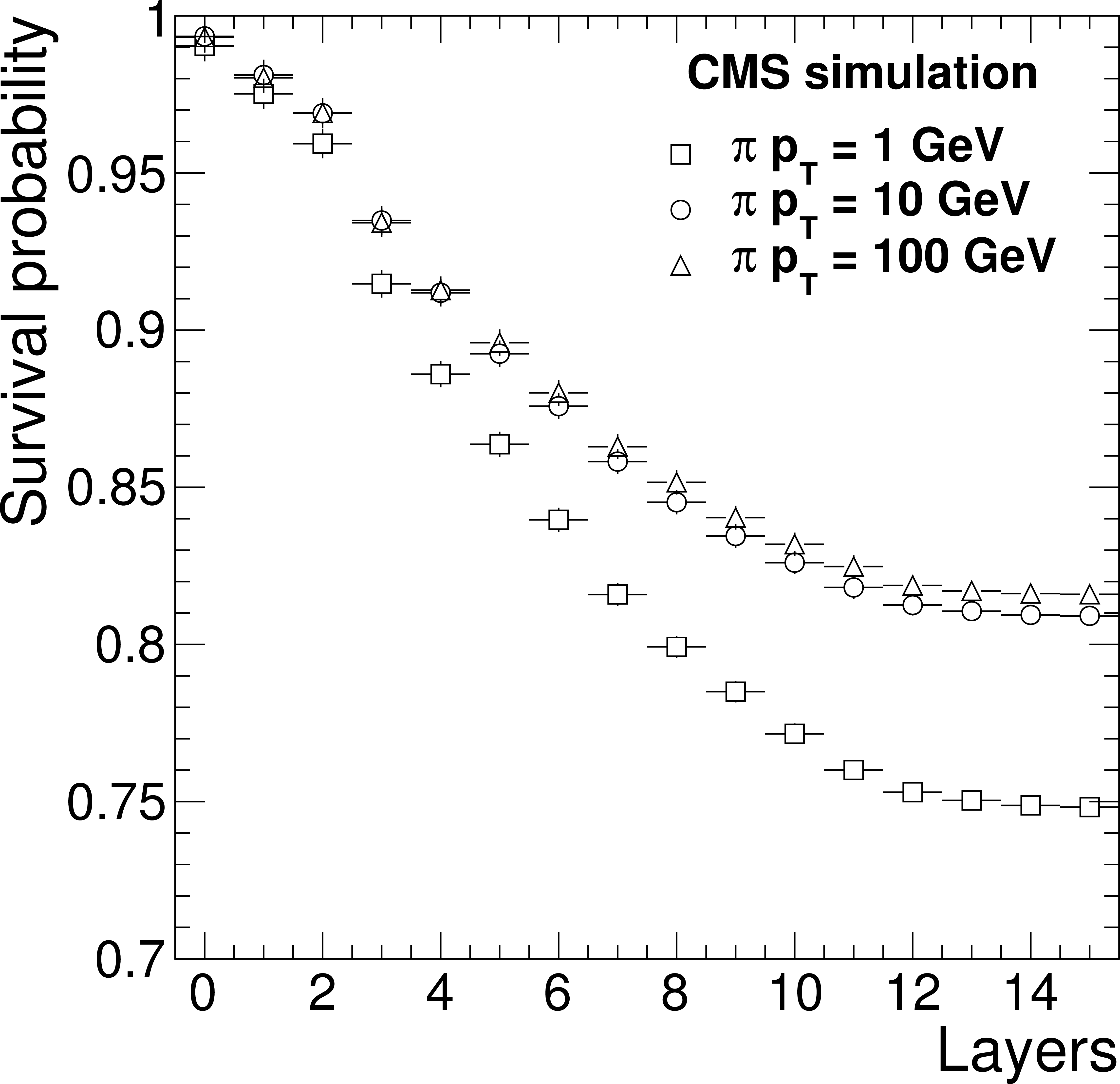
Figure 7:
Fraction of pions produced with $ {| \eta | }<2.5$ that do not undergo a nuclear interaction in the tracker volume, as a function of the number of traversed layers. |
png pdf |
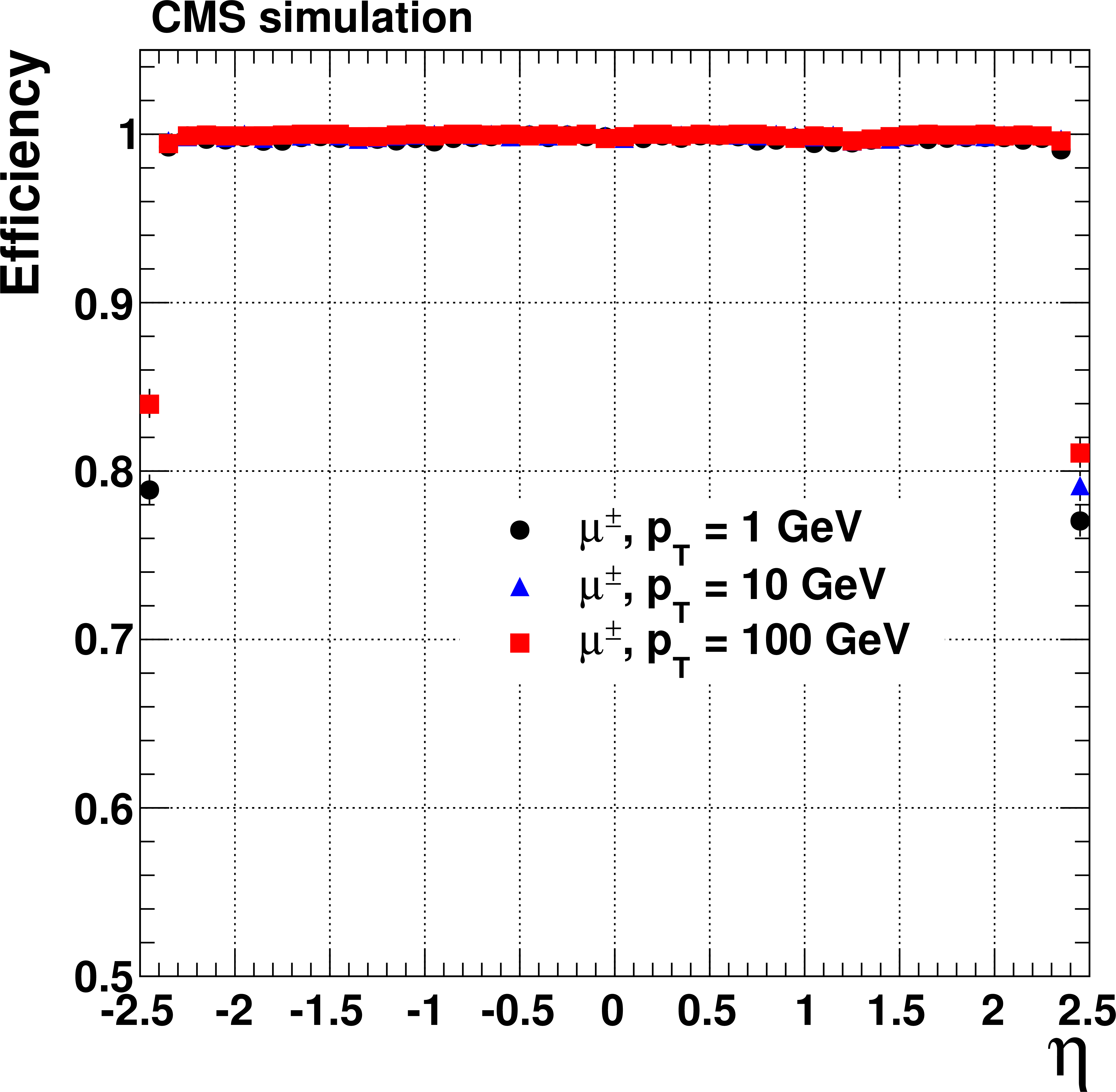
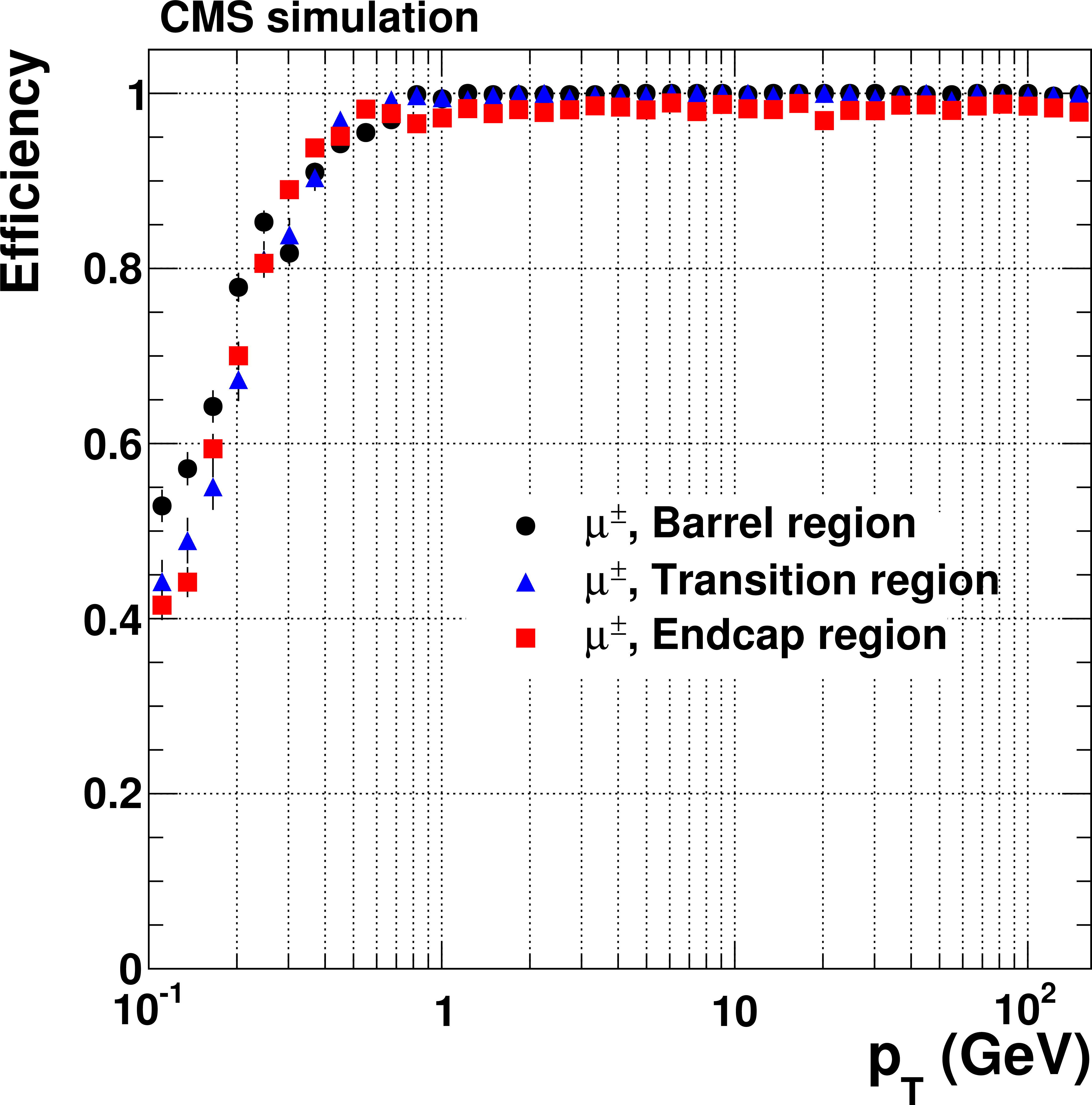
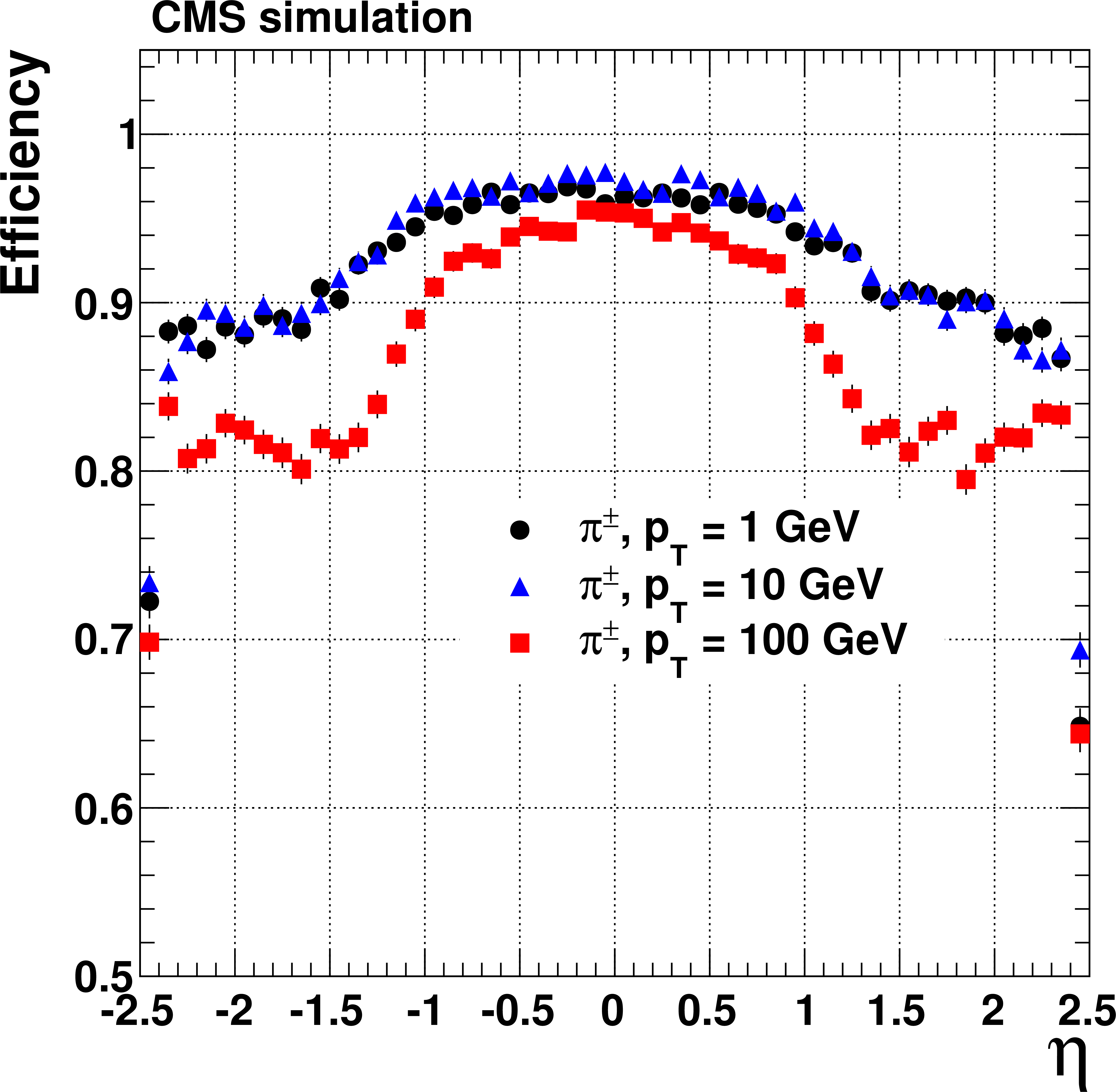
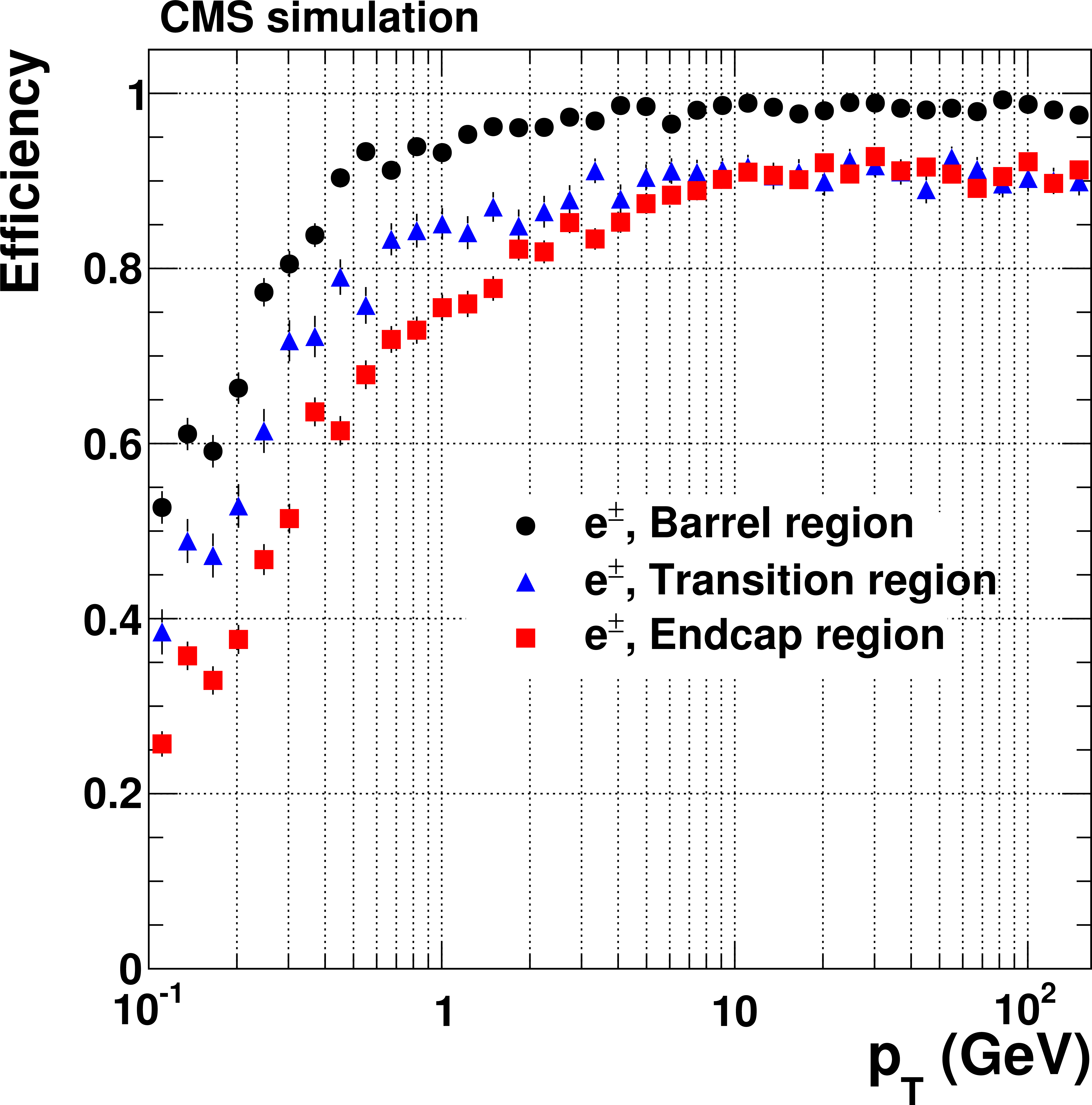
Figure 8-a:
Track reconstruction efficiencies for single, isolated muons (a, b), pions (c, d) and electrons (e, f) passing the high-purity quality requirements. Results are shown as a function of $\eta $ (a, c, e), for $ {p_{\mathrm {T}}} $ = 1, 10, and 100 GeV. They are also shown as a function of $ {p_{\mathrm {T}}} $ (b, d, f), for the barrel, transition, and endcap regions, which are defined by the $\eta $ intervals of 0-0.9, 0.9-1.4 and 1.4-2.5, respectively. |
png pdf |
Figure 8-b:
Track reconstruction efficiencies for single, isolated muons (a, b), pions (c, d) and electrons (e, f) passing the high-purity quality requirements. Results are shown as a function of $\eta $ (a, c, e), for $ {p_{\mathrm {T}}} $ = 1, 10, and 100 GeV. They are also shown as a function of $ {p_{\mathrm {T}}} $ (b, d, f), for the barrel, transition, and endcap regions, which are defined by the $\eta $ intervals of 0-0.9, 0.9-1.4 and 1.4-2.5, respectively. |
png pdf |
Figure 8-c:
Track reconstruction efficiencies for single, isolated muons (a, b), pions (c, d) and electrons (e, f) passing the high-purity quality requirements. Results are shown as a function of $\eta $ (a, c, e), for $ {p_{\mathrm {T}}} $ = 1, 10, and 100 GeV. They are also shown as a function of $ {p_{\mathrm {T}}} $ (b, d, f), for the barrel, transition, and endcap regions, which are defined by the $\eta $ intervals of 0-0.9, 0.9-1.4 and 1.4-2.5, respectively. |

png pdf |
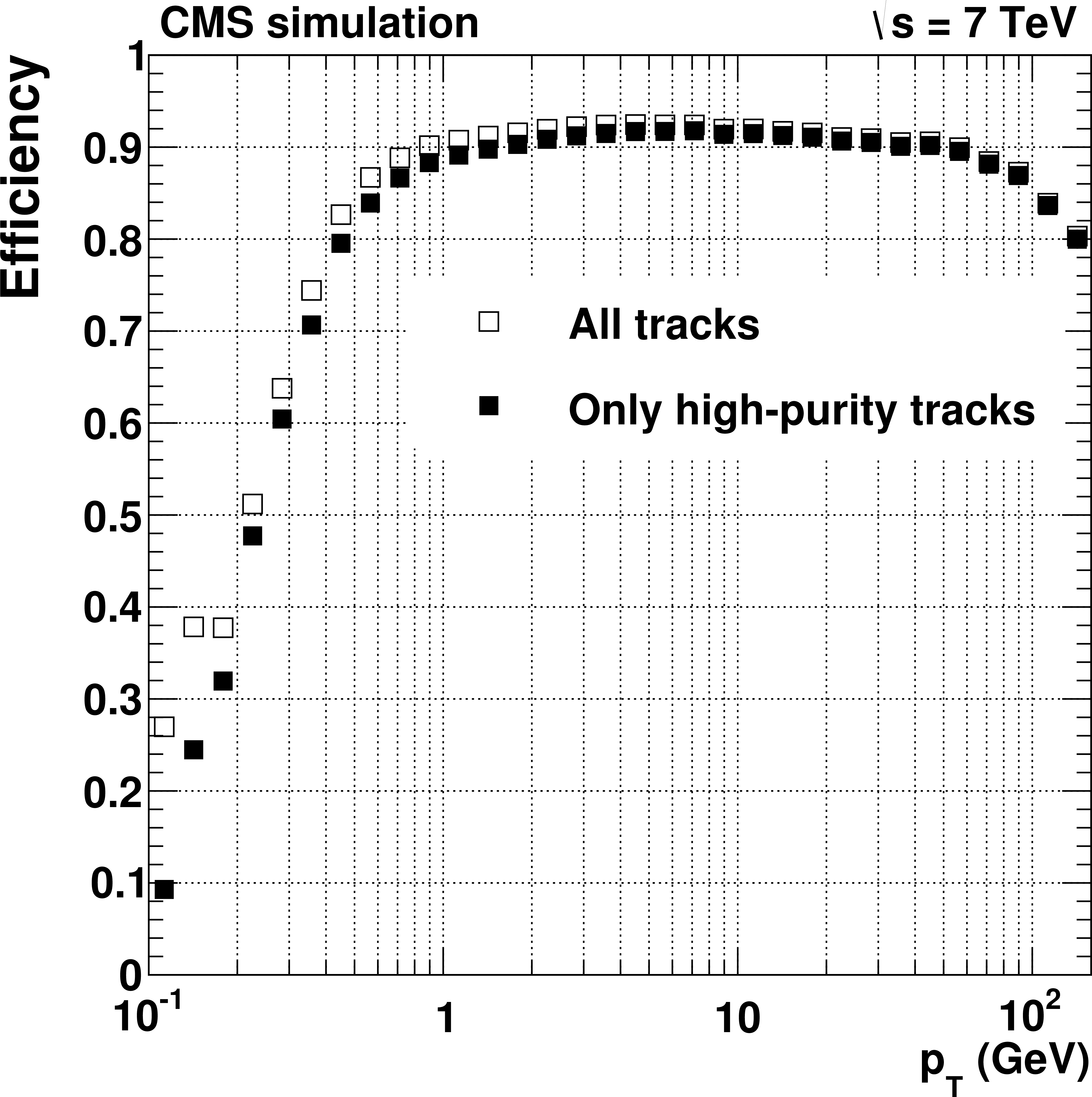
Figure 8-d:
Track reconstruction efficiencies for single, isolated muons (a, b), pions (c, d) and electrons (e, f) passing the high-purity quality requirements. Results are shown as a function of $\eta $ (a, c, e), for $ {p_{\mathrm {T}}} $ = 1, 10, and 100 GeV. They are also shown as a function of $ {p_{\mathrm {T}}} $ (b, d, f), for the barrel, transition, and endcap regions, which are defined by the $\eta $ intervals of 0-0.9, 0.9-1.4 and 1.4-2.5, respectively. |

png pdf |
Figure 8-e:
Track reconstruction efficiencies for single, isolated muons (a, b), pions (c, d) and electrons (e, f) passing the high-purity quality requirements. Results are shown as a function of $\eta $ (a, c, e), for $ {p_{\mathrm {T}}} $ = 1, 10, and 100 GeV. They are also shown as a function of $ {p_{\mathrm {T}}} $ (b, d, f), for the barrel, transition, and endcap regions, which are defined by the $\eta $ intervals of 0-0.9, 0.9-1.4 and 1.4-2.5, respectively. |
png pdf |
Figure 8-f:
Track reconstruction efficiencies for single, isolated muons (a, b), pions (c, d) and electrons (e, f) passing the high-purity quality requirements. Results are shown as a function of $\eta $ (a, c, e), for $ {p_{\mathrm {T}}} $ = 1, 10, and 100 GeV. They are also shown as a function of $ {p_{\mathrm {T}}} $ (b, d, f), for the barrel, transition, and endcap regions, which are defined by the $\eta $ intervals of 0-0.9, 0.9-1.4 and 1.4-2.5, respectively. |
png pdf |
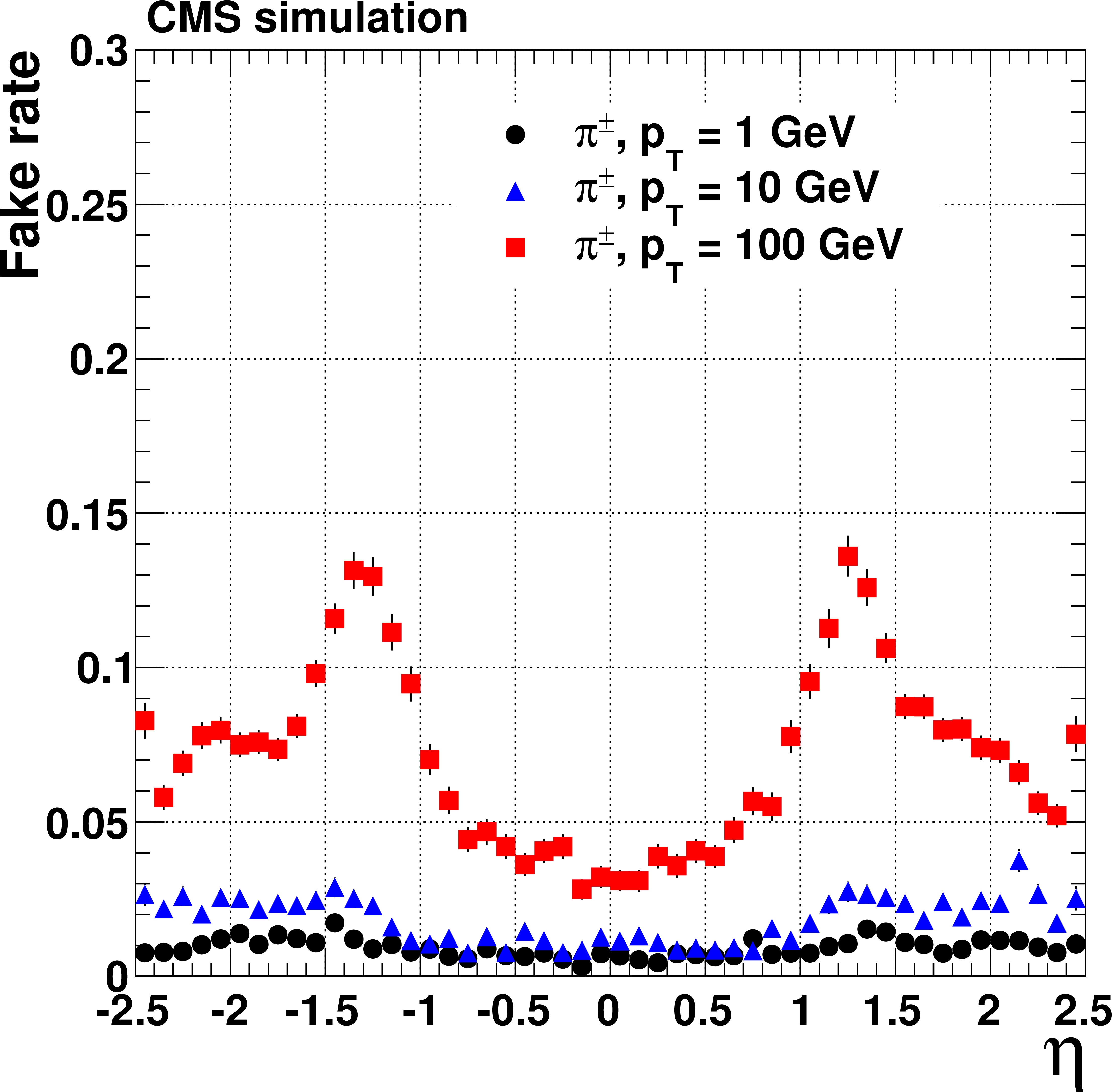
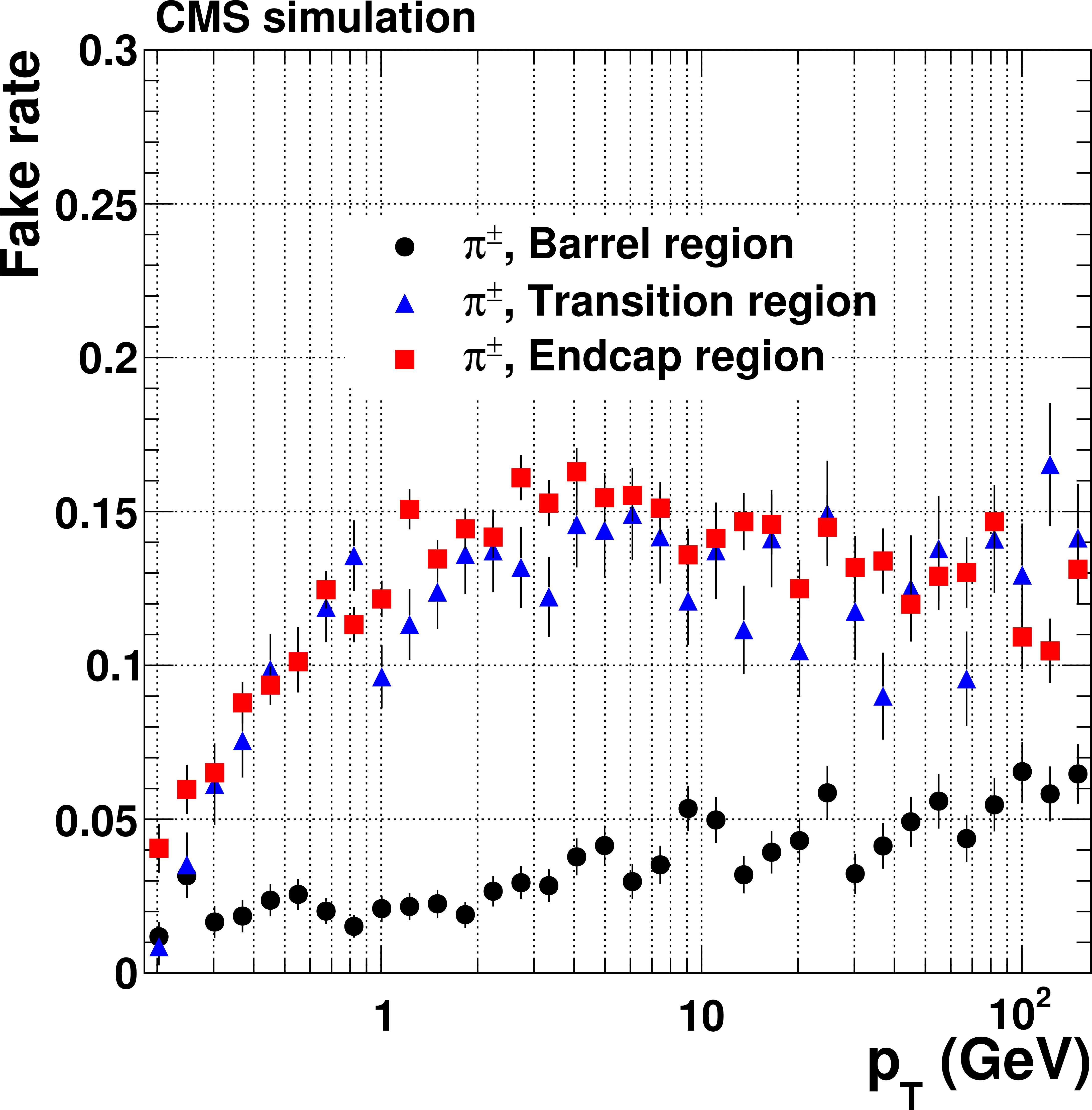
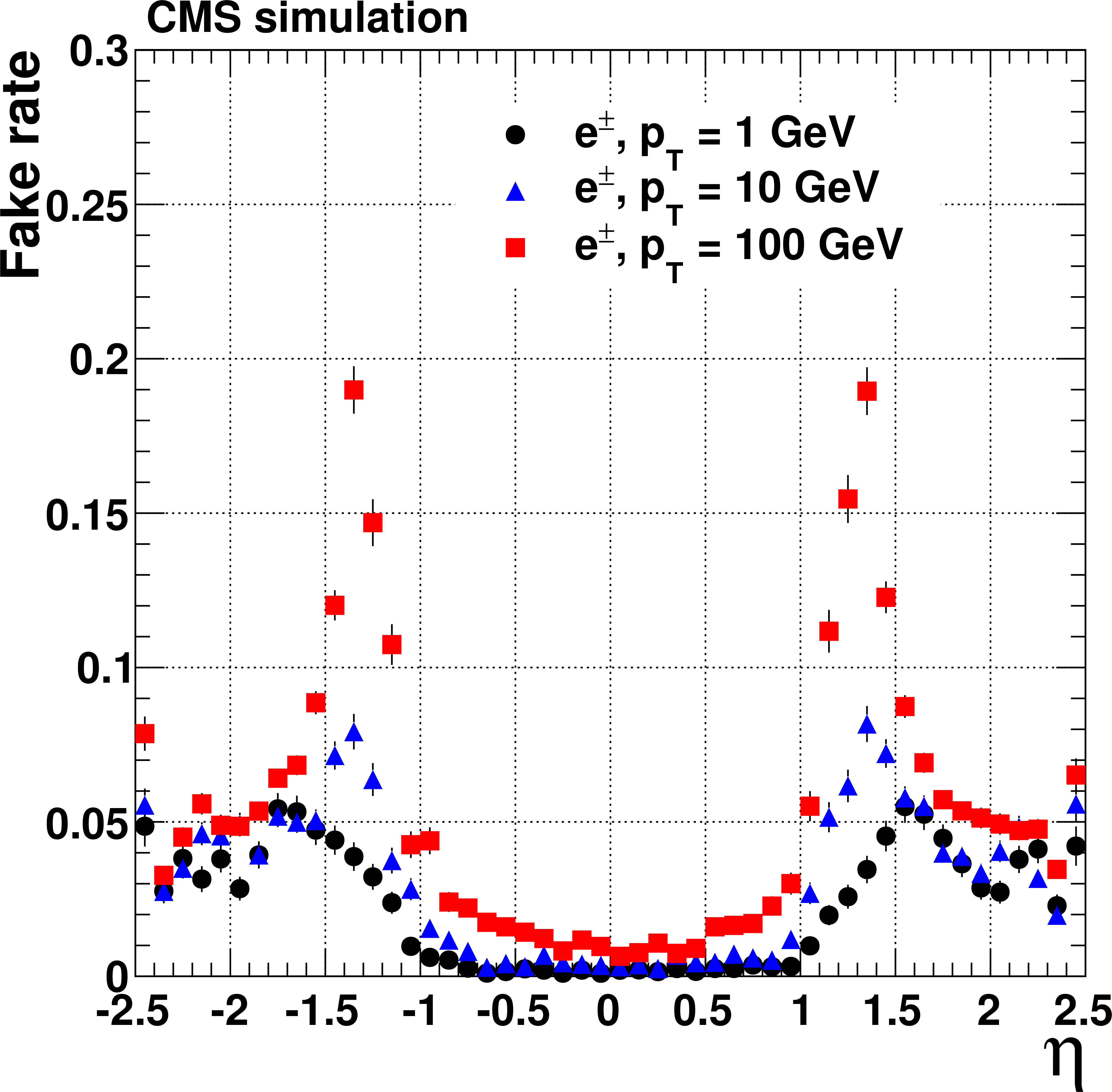
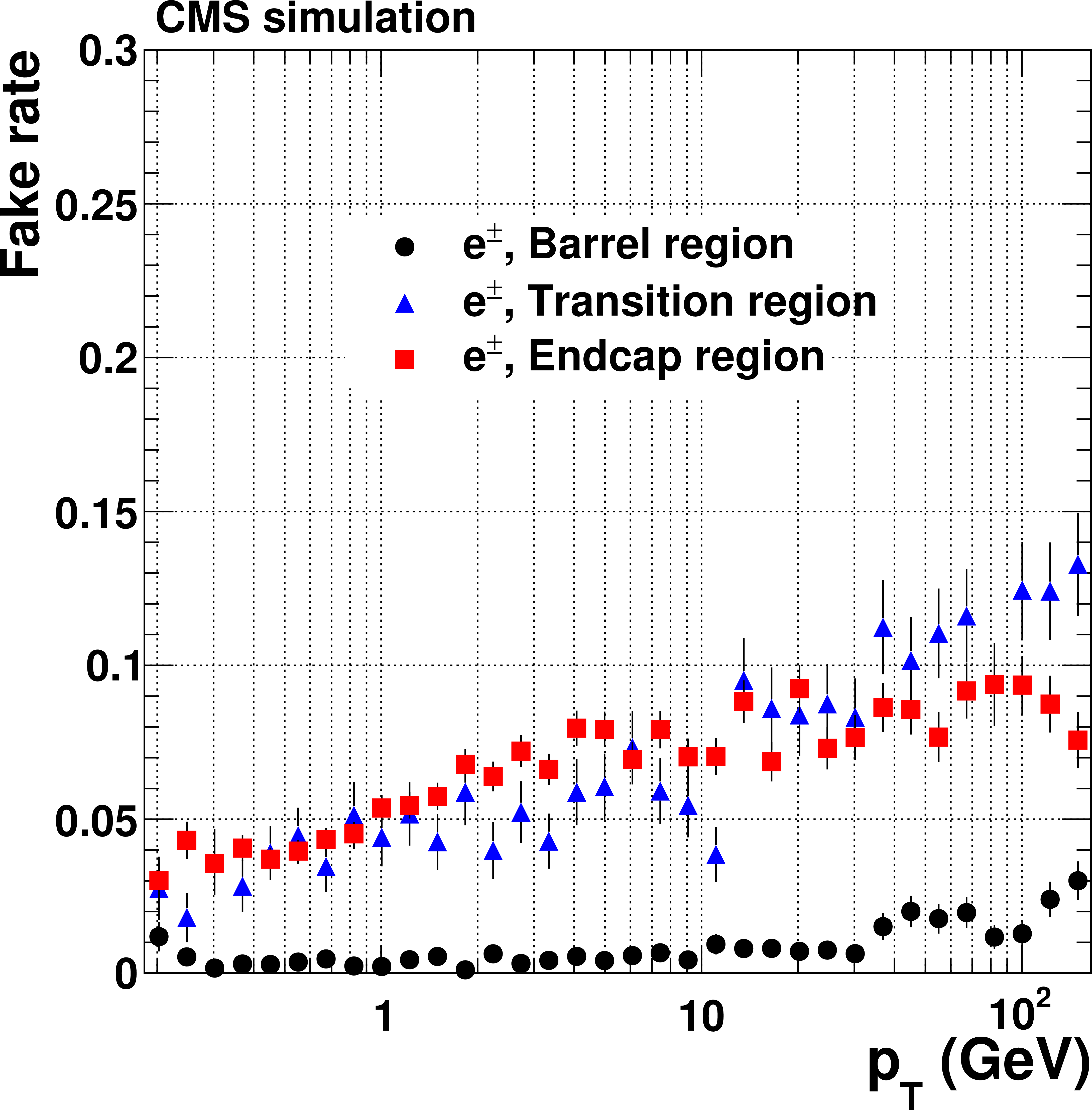
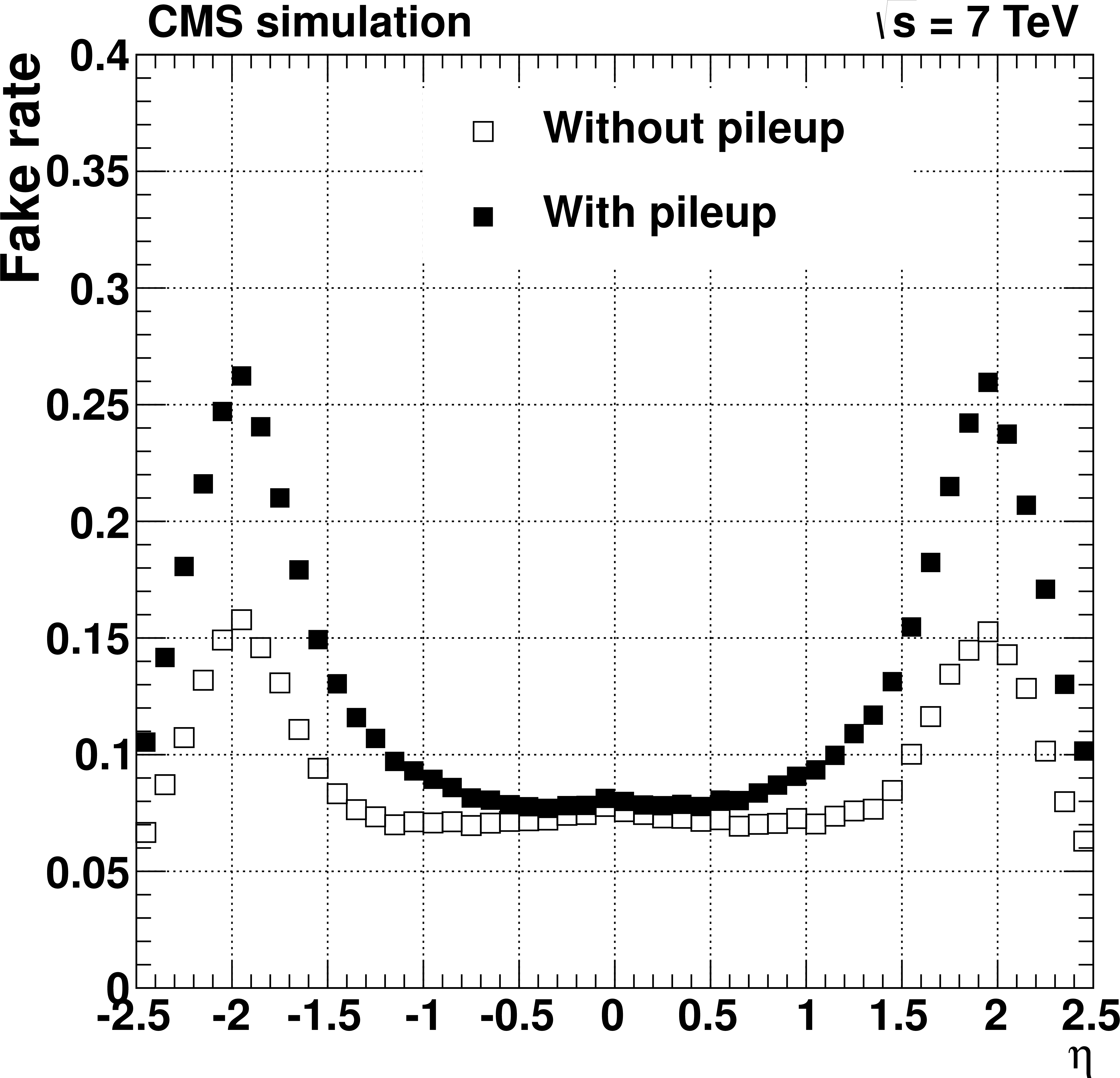
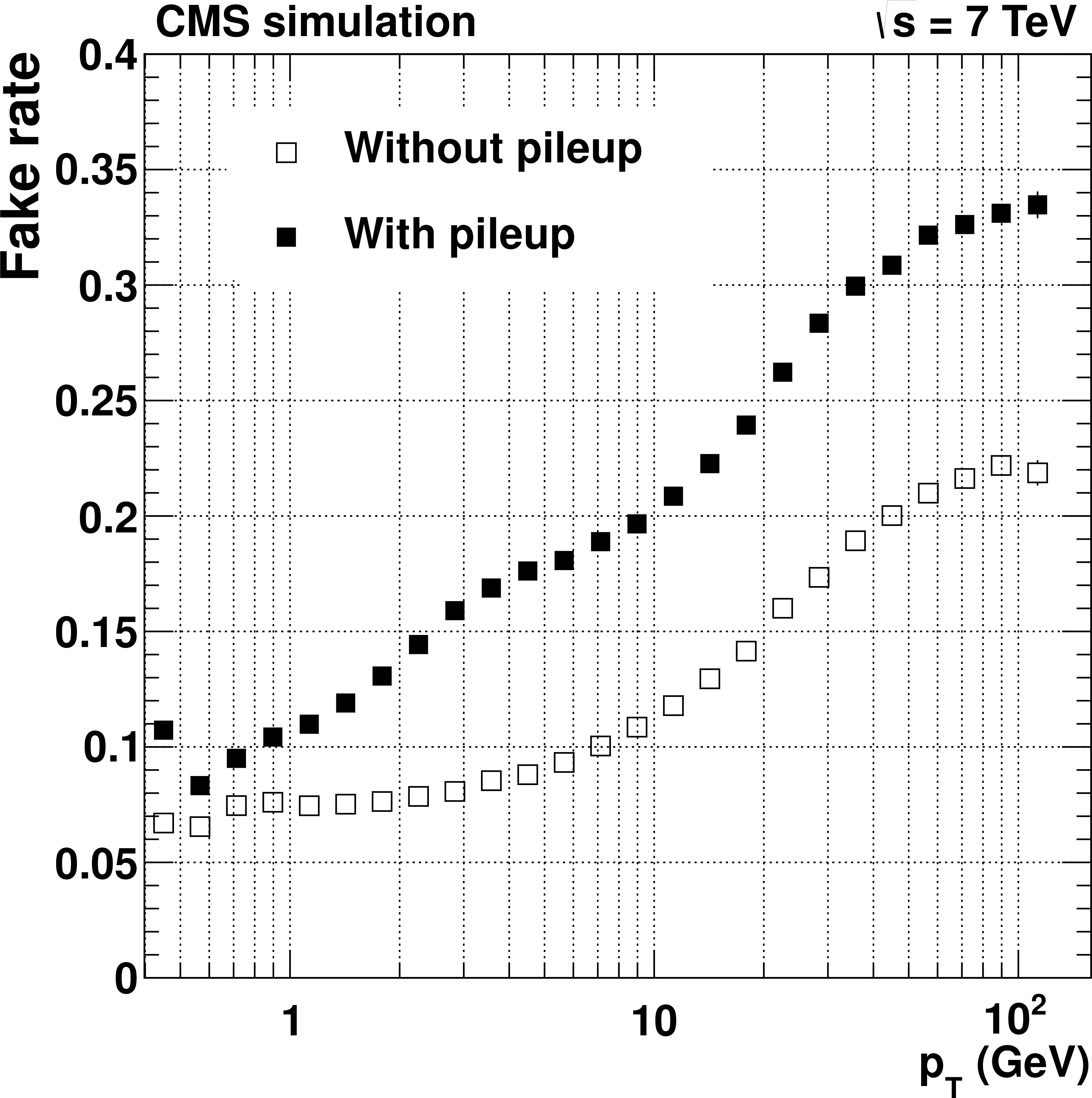
Figure 9-a:
Tracking fake rate for single, isolated pions (a, b) and electrons (c, d) passing high-purity quality requirements. Results are shown, as a function of the reconstructed $\eta $ (a, c), for generated $ {p_{\mathrm {T}}} = $ 1, 10, and 100 GeV. Results are also shown as a function of the reconstructed $ {p_{\mathrm {T}}} $ (b, d), for the barrel, transition, and endcap regions, which are defined by the $\eta $ intervals of 0-0.9, 0.9-1.4 and 1.4-2.5, respectively. The results for $ {p_{\mathrm {T}}} $ are obtained using particles generated with a flat distribution in $\ln {p_{\mathrm {T}}} $. NB The measured fake rate depends strongly on the $ {p_{\mathrm {T}}} $ distribution of the generated particles, since, for example, if no particles are generated in a given $ {p_{\mathrm {T}}} $ range, most tracks reconstructed in that range must necessarily be fake. The generated particles used to make the plots of fake rate versus $\eta $ have a different $ {p_{\mathrm {T}}} $ spectrum to those used to make the plots of fake rate versus $ {p_{\mathrm {T}}} $ , therefore the measured fake rates in these two sets of plots are not directly comparable. |
png pdf |
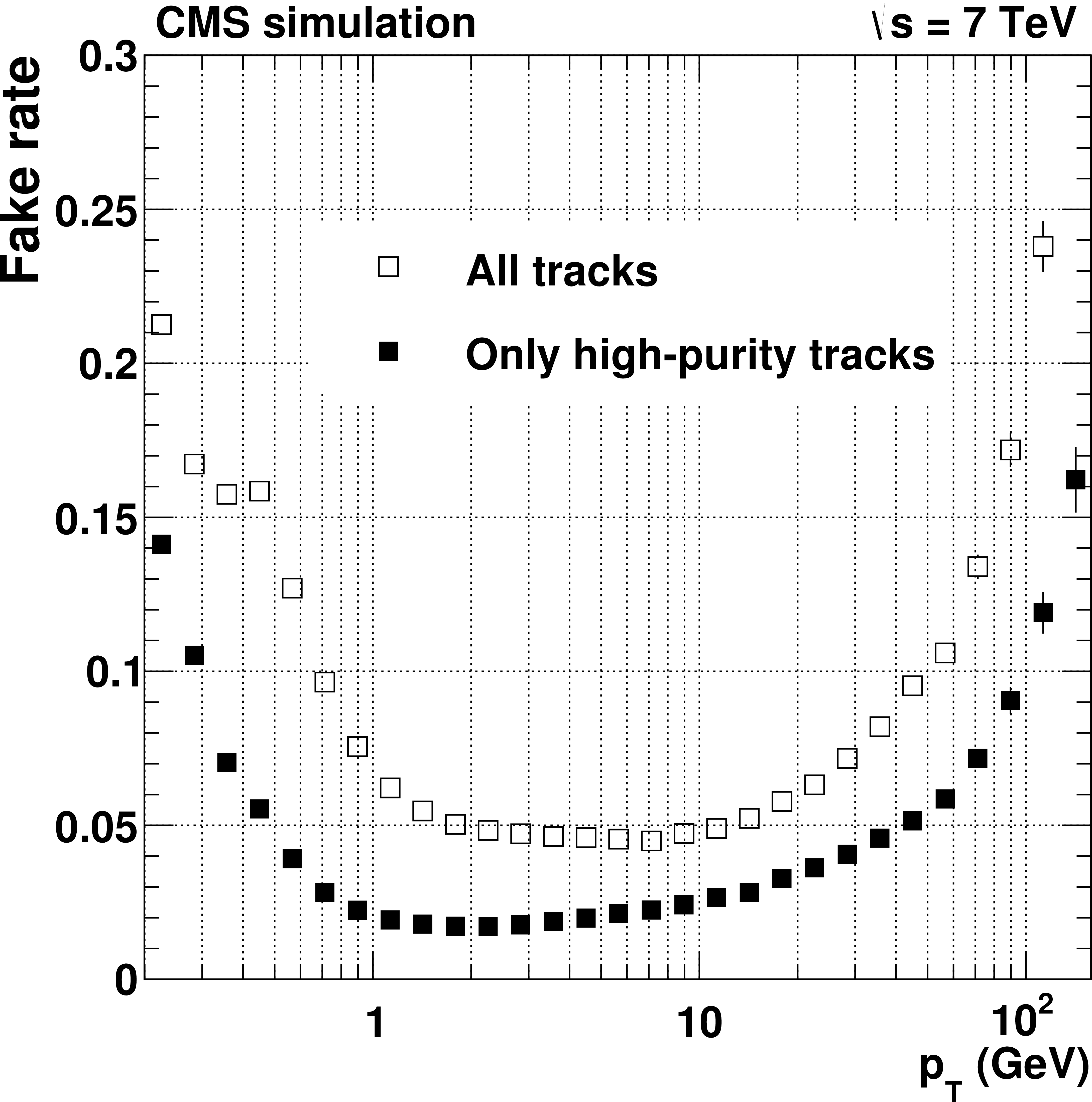
Figure 9-b:
Tracking fake rate for single, isolated pions (a, b) and electrons (c, d) passing high-purity quality requirements. Results are shown, as a function of the reconstructed $\eta $ (a, c), for generated $ {p_{\mathrm {T}}} = $ 1, 10, and 100 GeV. Results are also shown as a function of the reconstructed $ {p_{\mathrm {T}}} $ (b, d), for the barrel, transition, and endcap regions, which are defined by the $\eta $ intervals of 0-0.9, 0.9-1.4 and 1.4-2.5, respectively. The results for $ {p_{\mathrm {T}}} $ are obtained using particles generated with a flat distribution in $\ln {p_{\mathrm {T}}} $. NB The measured fake rate depends strongly on the $ {p_{\mathrm {T}}} $ distribution of the generated particles, since, for example, if no particles are generated in a given $ {p_{\mathrm {T}}} $ range, most tracks reconstructed in that range must necessarily be fake. The generated particles used to make the plots of fake rate versus $\eta $ have a different $ {p_{\mathrm {T}}} $ spectrum to those used to make the plots of fake rate versus $ {p_{\mathrm {T}}} $ , therefore the measured fake rates in these two sets of plots are not directly comparable. |
png pdf |
Figure 9-c:
Tracking fake rate for single, isolated pions (a, b) and electrons (c, d) passing high-purity quality requirements. Results are shown, as a function of the reconstructed $\eta $ (a, c), for generated $ {p_{\mathrm {T}}} = $ 1, 10, and 100 GeV. Results are also shown as a function of the reconstructed $ {p_{\mathrm {T}}} $ (b, d), for the barrel, transition, and endcap regions, which are defined by the $\eta $ intervals of 0-0.9, 0.9-1.4 and 1.4-2.5, respectively. The results for $ {p_{\mathrm {T}}} $ are obtained using particles generated with a flat distribution in $\ln {p_{\mathrm {T}}} $. NB The measured fake rate depends strongly on the $ {p_{\mathrm {T}}} $ distribution of the generated particles, since, for example, if no particles are generated in a given $ {p_{\mathrm {T}}} $ range, most tracks reconstructed in that range must necessarily be fake. The generated particles used to make the plots of fake rate versus $\eta $ have a different $ {p_{\mathrm {T}}} $ spectrum to those used to make the plots of fake rate versus $ {p_{\mathrm {T}}} $ , therefore the measured fake rates in these two sets of plots are not directly comparable. |
png pdf |
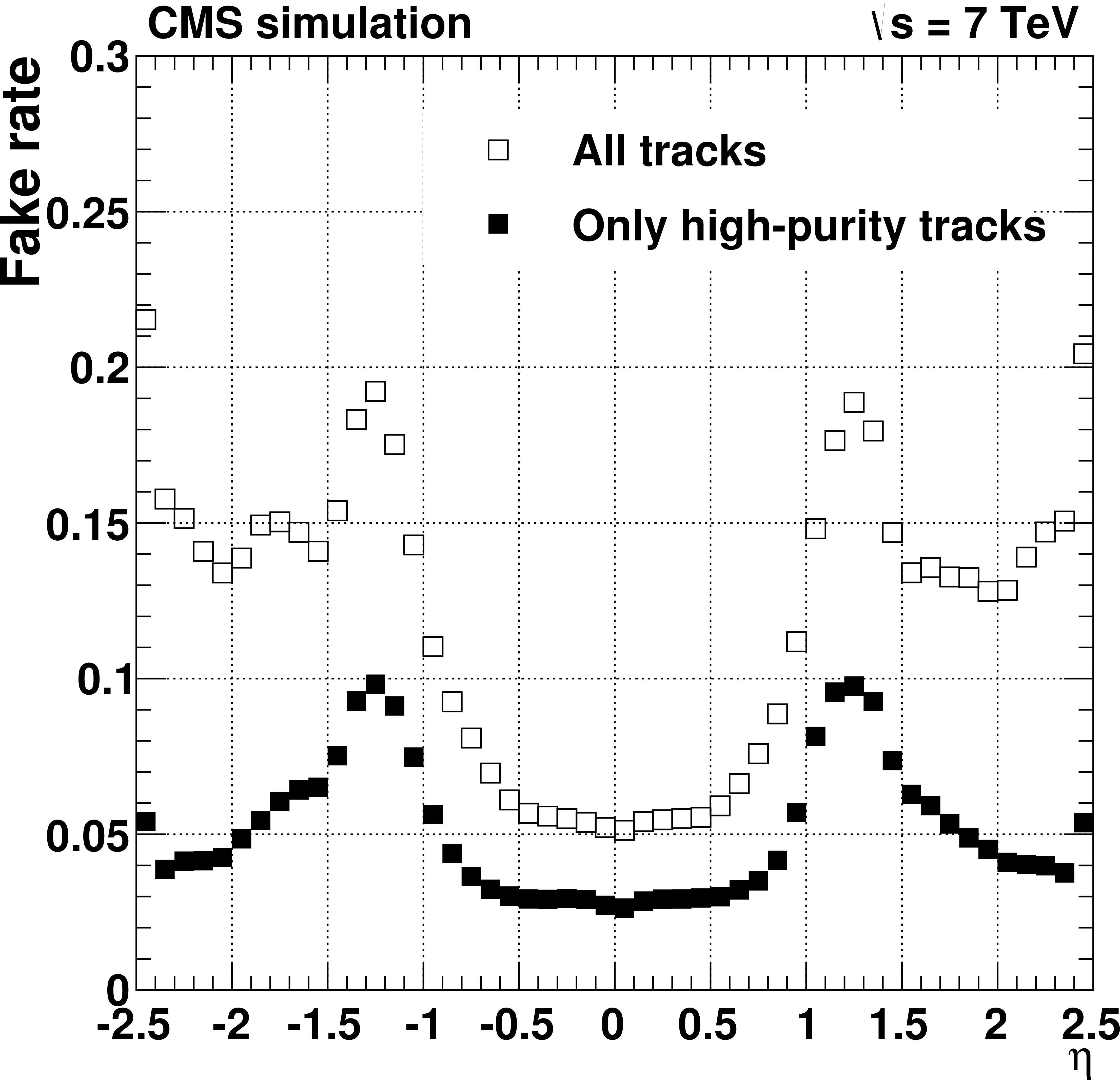
Figure 9-d:
Tracking fake rate for single, isolated pions (a, b) and electrons (c, d) passing high-purity quality requirements. Results are shown, as a function of the reconstructed $\eta $ (a, c), for generated $ {p_{\mathrm {T}}} = $ 1, 10, and 100 GeV. Results are also shown as a function of the reconstructed $ {p_{\mathrm {T}}} $ (b, d), for the barrel, transition, and endcap regions, which are defined by the $\eta $ intervals of 0-0.9, 0.9-1.4 and 1.4-2.5, respectively. The results for $ {p_{\mathrm {T}}} $ are obtained using particles generated with a flat distribution in $\ln {p_{\mathrm {T}}} $. NB The measured fake rate depends strongly on the $ {p_{\mathrm {T}}} $ distribution of the generated particles, since, for example, if no particles are generated in a given $ {p_{\mathrm {T}}} $ range, most tracks reconstructed in that range must necessarily be fake. The generated particles used to make the plots of fake rate versus $\eta $ have a different $ {p_{\mathrm {T}}} $ spectrum to those used to make the plots of fake rate versus $ {p_{\mathrm {T}}} $ , therefore the measured fake rates in these two sets of plots are not directly comparable. |
png pdf |
Figure 10-a:
Tracking efficiency (a, b) and fake rate (c, d) for simulated $ \mathrm{ t \bar{t} } $ events that include superimposed pileup collisions. The number of pileup interactions superimposed on each simulated event is generated randomly from a Poisson distribution with mean value of 8. Plots are for all reconstructed tracks, and also for the subset of tracks passing high-purity requirements. The efficiency and fake rate plots are plotted for $ {| \eta | }< $ 2.5, and the efficiency for charged particles refers to those generated less than 3 cm (30 cm) from the centre of the beam spot in $r$ ($z$) directions. The efficiency as a function of $\eta $ is for generated particles with $ {p_{\mathrm {T}}} > $ 0.9 GeV. |
png pdf |
Figure 10-b:
Tracking efficiency (a, b) and fake rate (c, d) for simulated $ \mathrm{ t \bar{t} } $ events that include superimposed pileup collisions. The number of pileup interactions superimposed on each simulated event is generated randomly from a Poisson distribution with mean value of 8. Plots are for all reconstructed tracks, and also for the subset of tracks passing high-purity requirements. The efficiency and fake rate plots are plotted for $ {| \eta | }< $ 2.5, and the efficiency for charged particles refers to those generated less than 3 cm (30 cm) from the centre of the beam spot in $r$ ($z$) directions. The efficiency as a function of $\eta $ is for generated particles with $ {p_{\mathrm {T}}} > $ 0.9 GeV. |
png pdf |
Figure 10-c:
Tracking efficiency (a, b) and fake rate (c, d) for simulated $ \mathrm{ t \bar{t} } $ events that include superimposed pileup collisions. The number of pileup interactions superimposed on each simulated event is generated randomly from a Poisson distribution with mean value of 8. Plots are for all reconstructed tracks, and also for the subset of tracks passing high-purity requirements. The efficiency and fake rate plots are plotted for $ {| \eta | }< $ 2.5, and the efficiency for charged particles refers to those generated less than 3 cm (30 cm) from the centre of the beam spot in $r$ ($z$) directions. The efficiency as a function of $\eta $ is for generated particles with $ {p_{\mathrm {T}}} > $ 0.9 GeV. |
png pdf |
Figure 10-d:
Tracking efficiency (a, b) and fake rate (c, d) for simulated $ \mathrm{ t \bar{t} } $ events that include superimposed pileup collisions. The number of pileup interactions superimposed on each simulated event is generated randomly from a Poisson distribution with mean value of 8. Plots are for all reconstructed tracks, and also for the subset of tracks passing high-purity requirements. The efficiency and fake rate plots are plotted for $ {| \eta | }< $ 2.5, and the efficiency for charged particles refers to those generated less than 3 cm (30 cm) from the centre of the beam spot in $r$ ($z$) directions. The efficiency as a function of $\eta $ is for generated particles with $ {p_{\mathrm {T}}} > $ 0.9 GeV. |
png pdf |
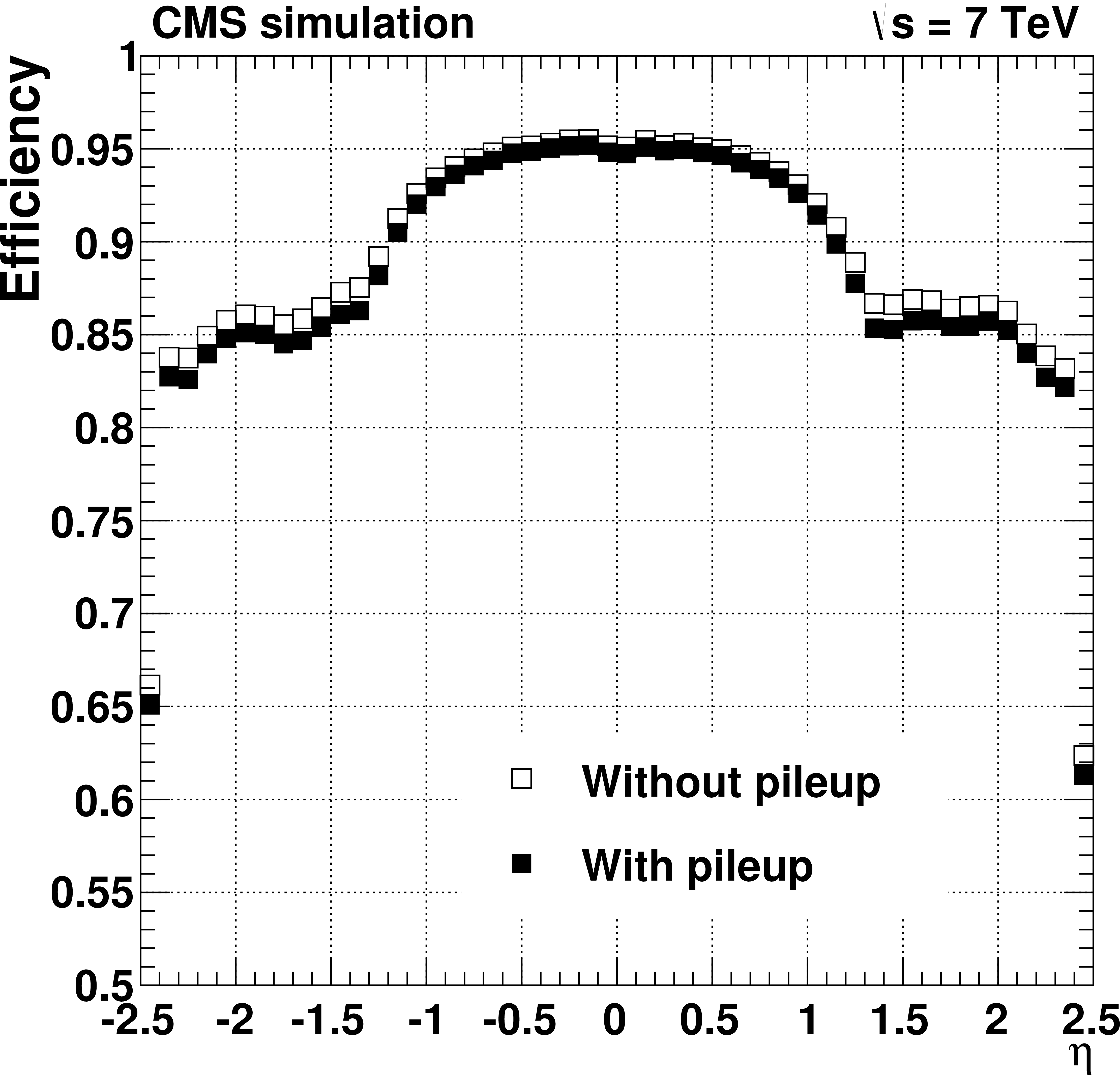
Figure 11-a:
Tracking efficiency (a, b) and fake rate (c, d) for $ \mathrm{ t \bar{t} } $ events simulated with and without superimposed pileup collisions. The number of pileup interactions superimposed on each simulated event is generated randomly from a Poisson distribution with mean value of 8. Plots are produced for the subset of tracks passing the high-purity quality requirements. The efficiency and fake rate plots cover $ {| \eta | }<$ 2.5. The efficiency results are for charged particles produced less than 3 cm (30 cm) from the centre of the beam spot in $r$ ($z$) directions. The efficiency as a function of $\eta $ is for generated particles with $ {p_{\mathrm {T}}} > $ 0.9 GeV. |
png pdf |
Figure 11-b:
Tracking efficiency (a, b) and fake rate (c, d) for $ \mathrm{ t \bar{t} } $ events simulated with and without superimposed pileup collisions. The number of pileup interactions superimposed on each simulated event is generated randomly from a Poisson distribution with mean value of 8. Plots are produced for the subset of tracks passing the high-purity quality requirements. The efficiency and fake rate plots cover $ {| \eta | }<$ 2.5. The efficiency results are for charged particles produced less than 3 cm (30 cm) from the centre of the beam spot in $r$ ($z$) directions. The efficiency as a function of $\eta $ is for generated particles with $ {p_{\mathrm {T}}} > $ 0.9 GeV. |
png pdf |
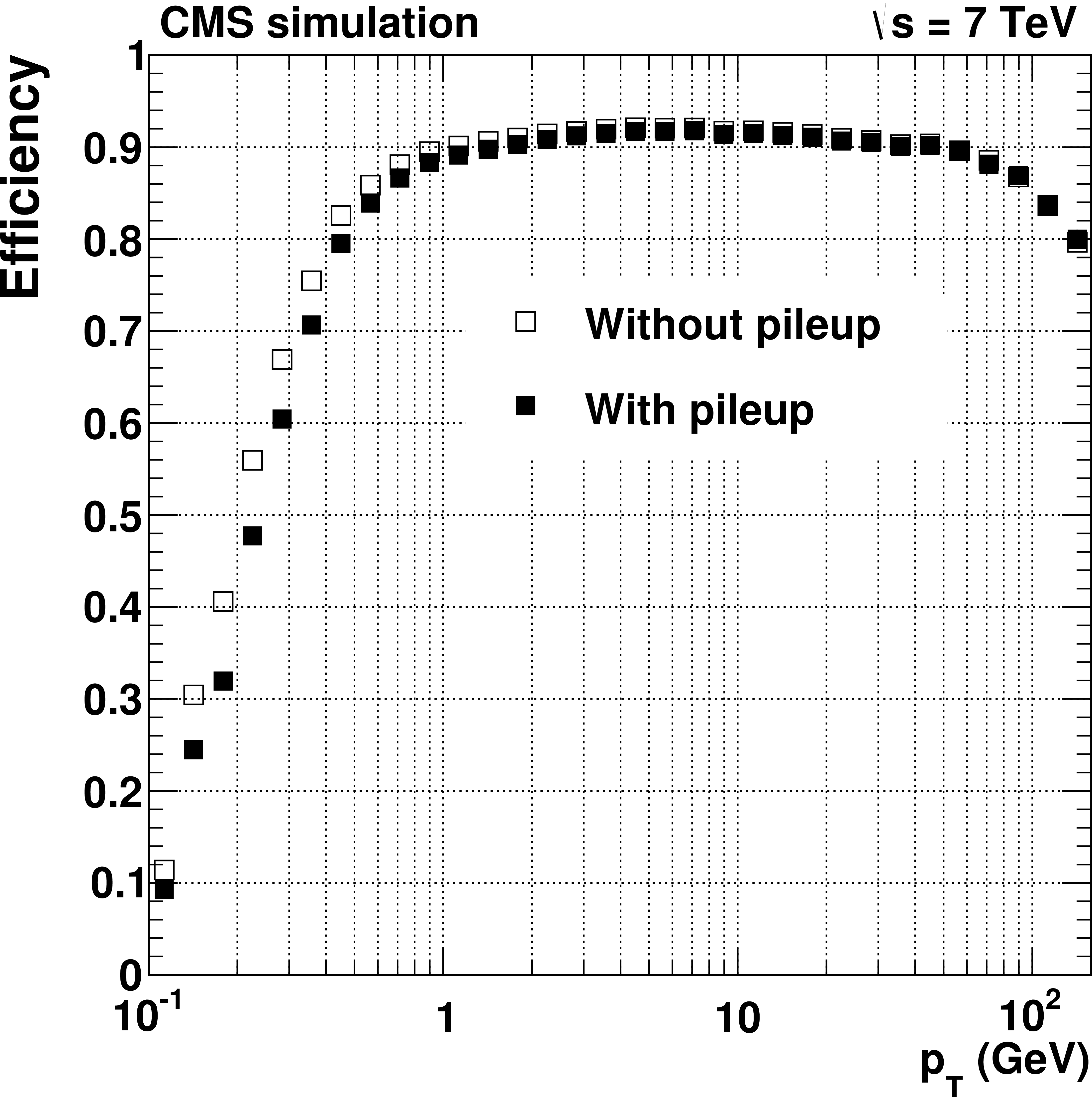
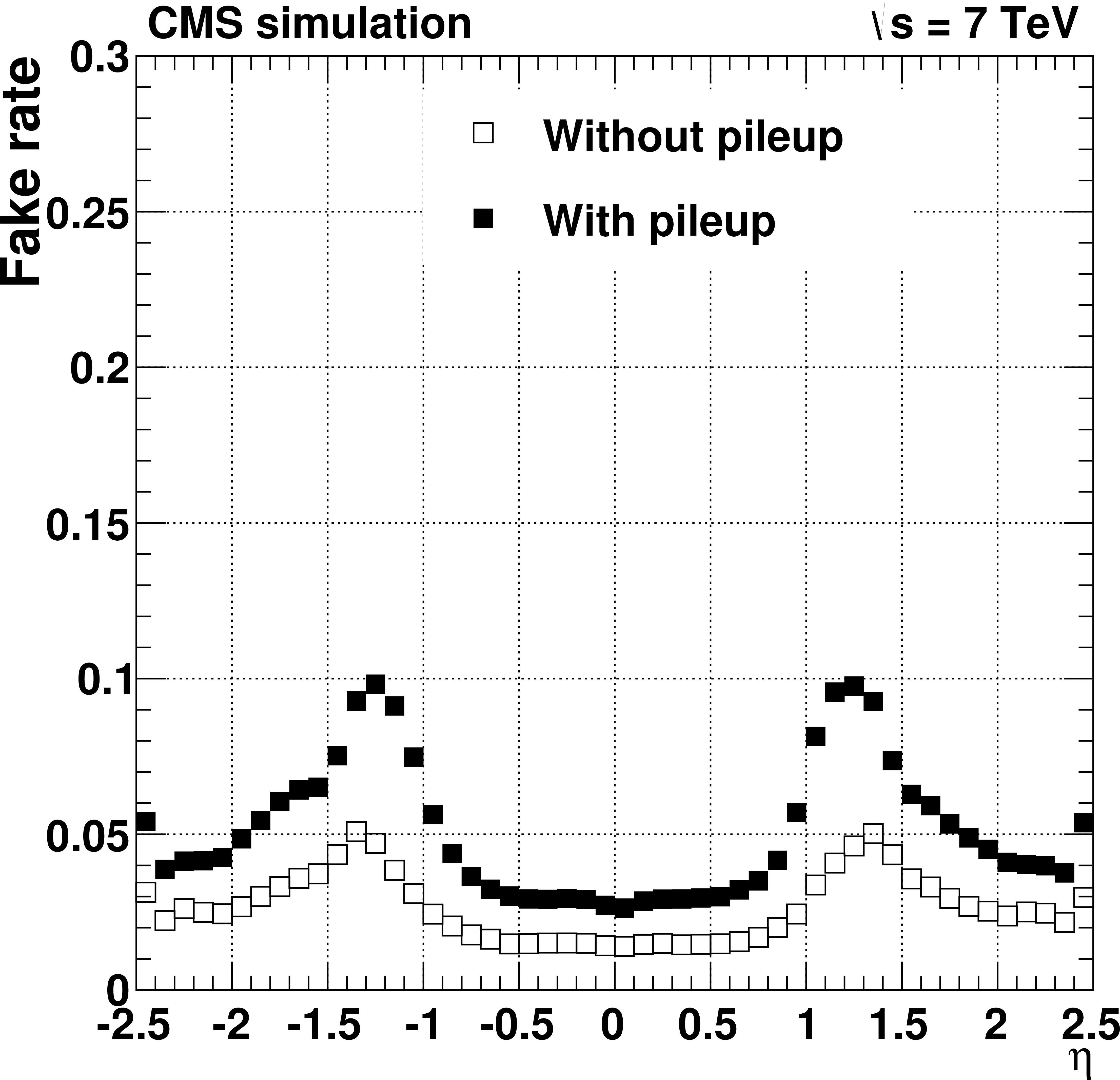
Figure 11-c:
Tracking efficiency (a, b) and fake rate (c, d) for $ \mathrm{ t \bar{t} } $ events simulated with and without superimposed pileup collisions. The number of pileup interactions superimposed on each simulated event is generated randomly from a Poisson distribution with mean value of 8. Plots are produced for the subset of tracks passing the high-purity quality requirements. The efficiency and fake rate plots cover $ {| \eta | }<$ 2.5. The efficiency results are for charged particles produced less than 3 cm (30 cm) from the centre of the beam spot in $r$ ($z$) directions. The efficiency as a function of $\eta $ is for generated particles with $ {p_{\mathrm {T}}} > $ 0.9 GeV. |

png pdf |
Figure 11-d:
Tracking efficiency (a, b) and fake rate (c, d) for $ \mathrm{ t \bar{t} } $ events simulated with and without superimposed pileup collisions. The number of pileup interactions superimposed on each simulated event is generated randomly from a Poisson distribution with mean value of 8. Plots are produced for the subset of tracks passing the high-purity quality requirements. The efficiency and fake rate plots cover $ {| \eta | }<$ 2.5. The efficiency results are for charged particles produced less than 3 cm (30 cm) from the centre of the beam spot in $r$ ($z$) directions. The efficiency as a function of $\eta $ is for generated particles with $ {p_{\mathrm {T}}} > $ 0.9 GeV. |
png pdf |
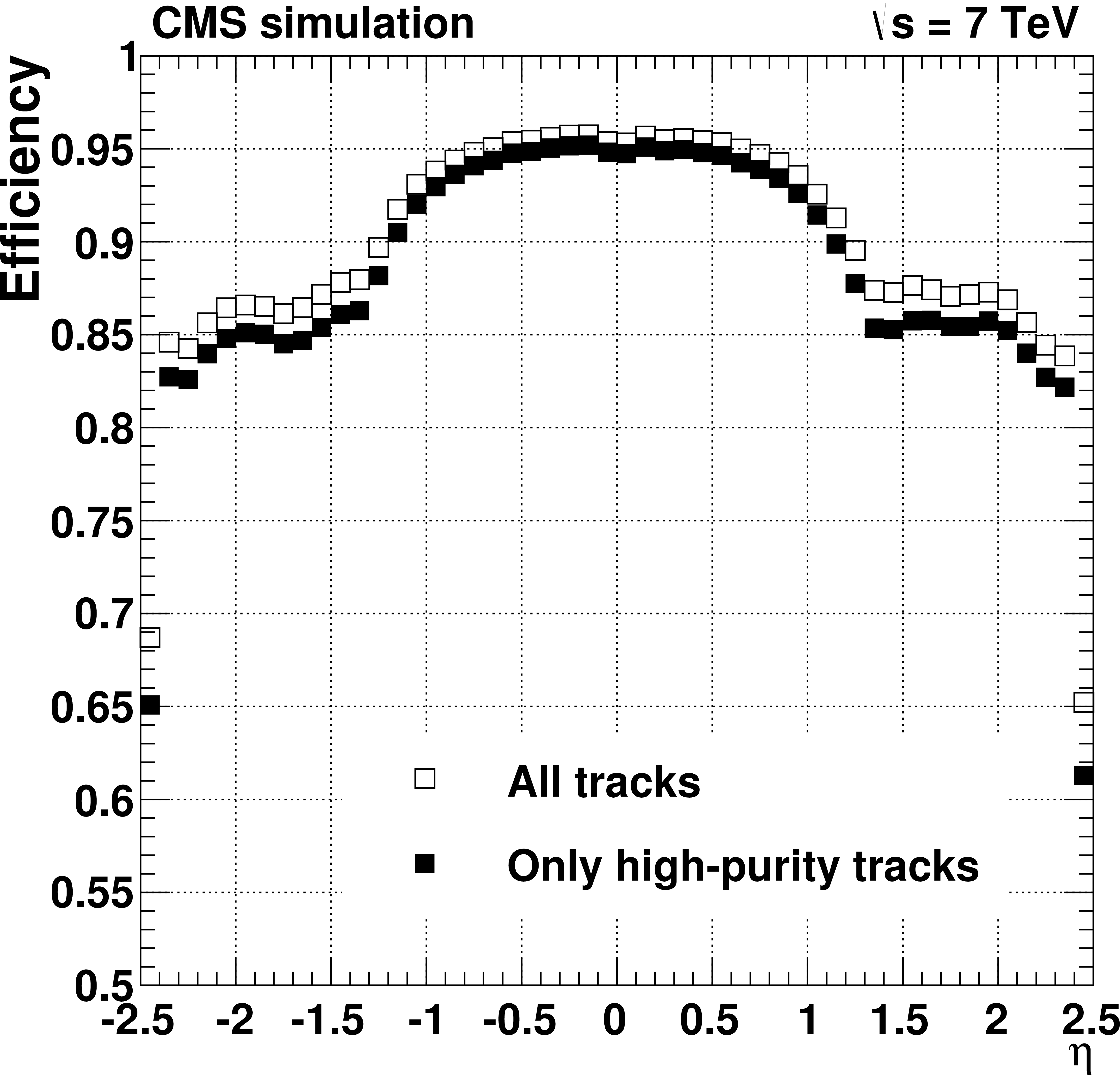
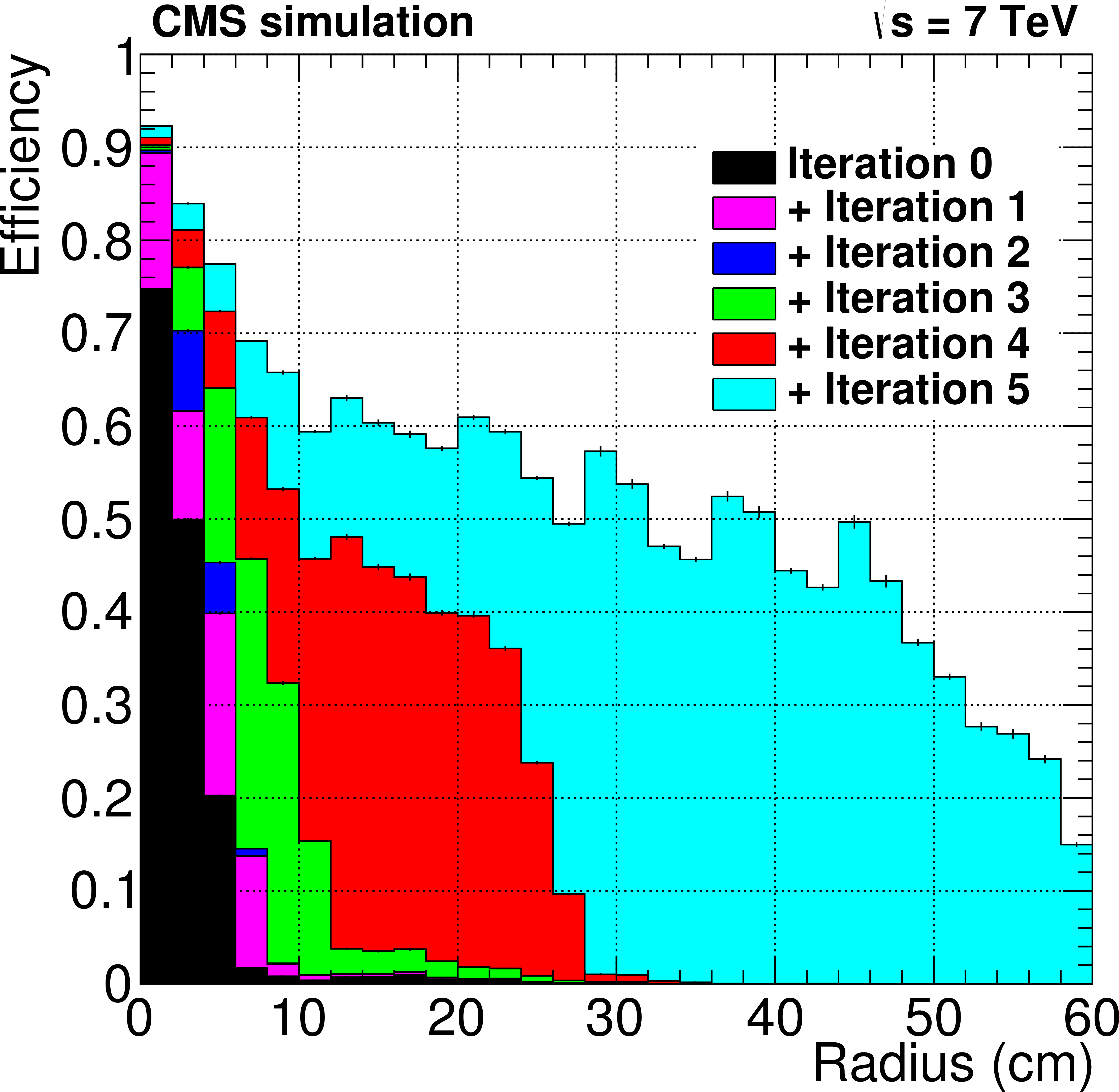
Figure 12:
Cumulative contributions to the overall tracking performance from the six iterations in track reconstruction. The tracking efficiency for simulated $ \mathrm{ t \bar{t} } $ events is shown as a function of transverse distance ($r$) from the beam axis to the production point of each particle, for tracks with $ {p_{\mathrm {T}}} >$ 0.9 GeV and $ {| \eta | }< $ 2.5, transverse (longitudinal) impact parameter $<$ 60 (30) cm . The reconstructed tracks are required to pass the high-purity quality requirements. |

png pdf |
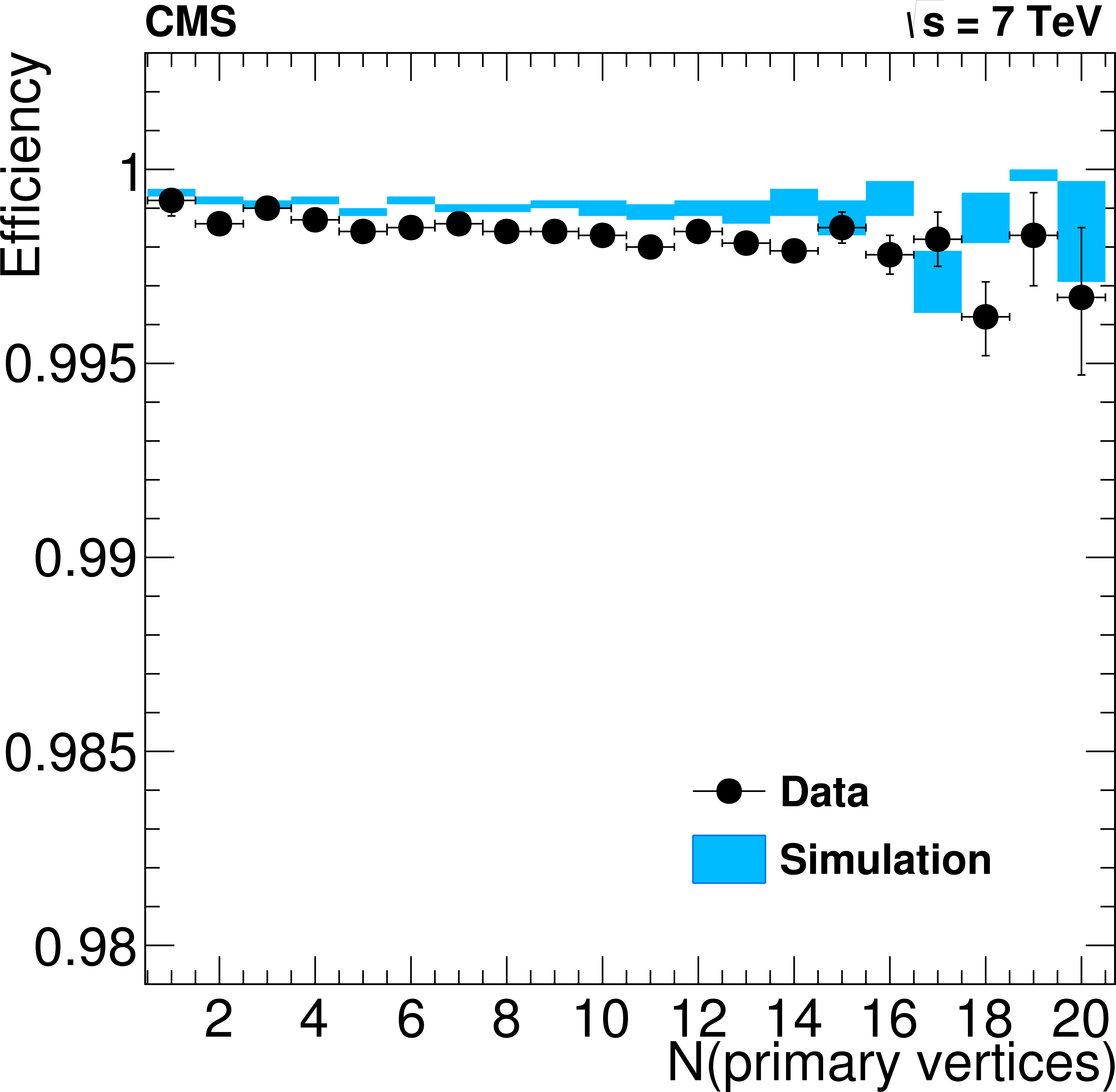
Figure 13-a:
Tracking efficiency measured with a tag-and-probe technique, for muons from $ {\mathrm {Z}}$ decays, as a function of the muon $\eta $ (a) and the number of reconstructed primary vertices in the event (b) for data (black dots) and simulation (blue bands). |
png pdf |
Figure 13-b:
Tracking efficiency measured with a tag-and-probe technique, for muons from $ {\mathrm {Z}}$ decays, as a function of the muon $\eta $ (a) and the number of reconstructed primary vertices in the event (b) for data (black dots) and simulation (blue bands). |
png pdf |
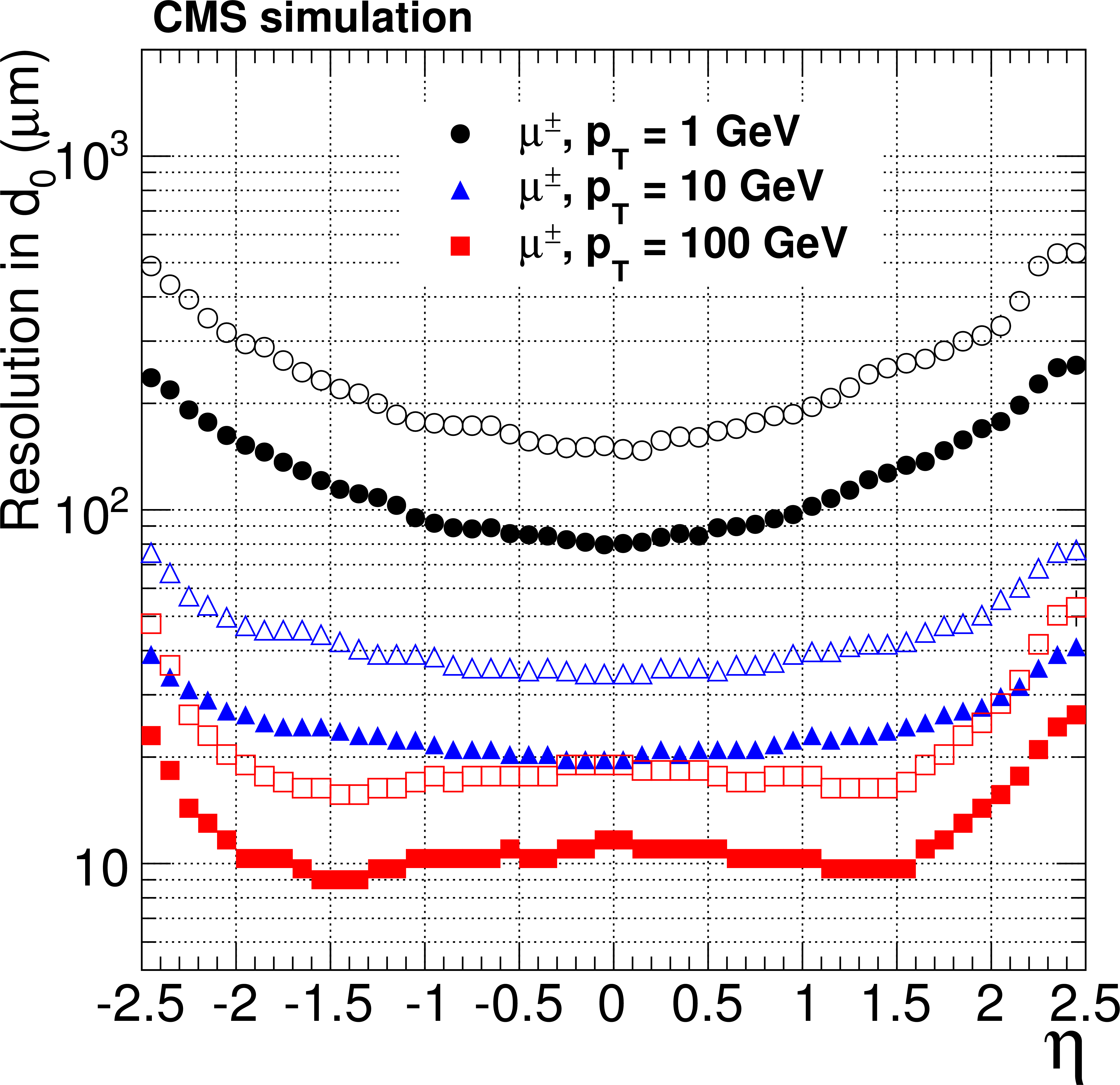
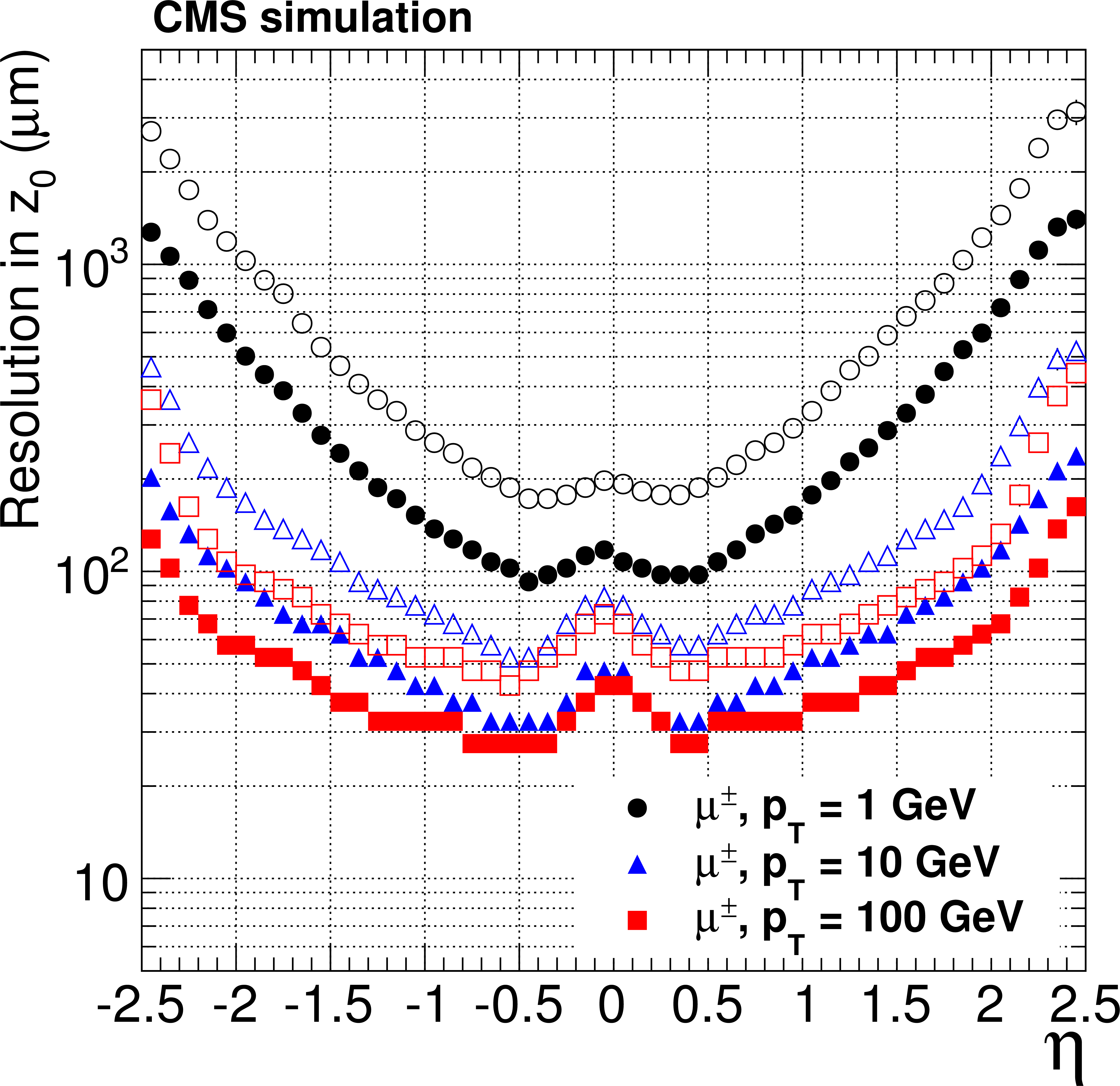
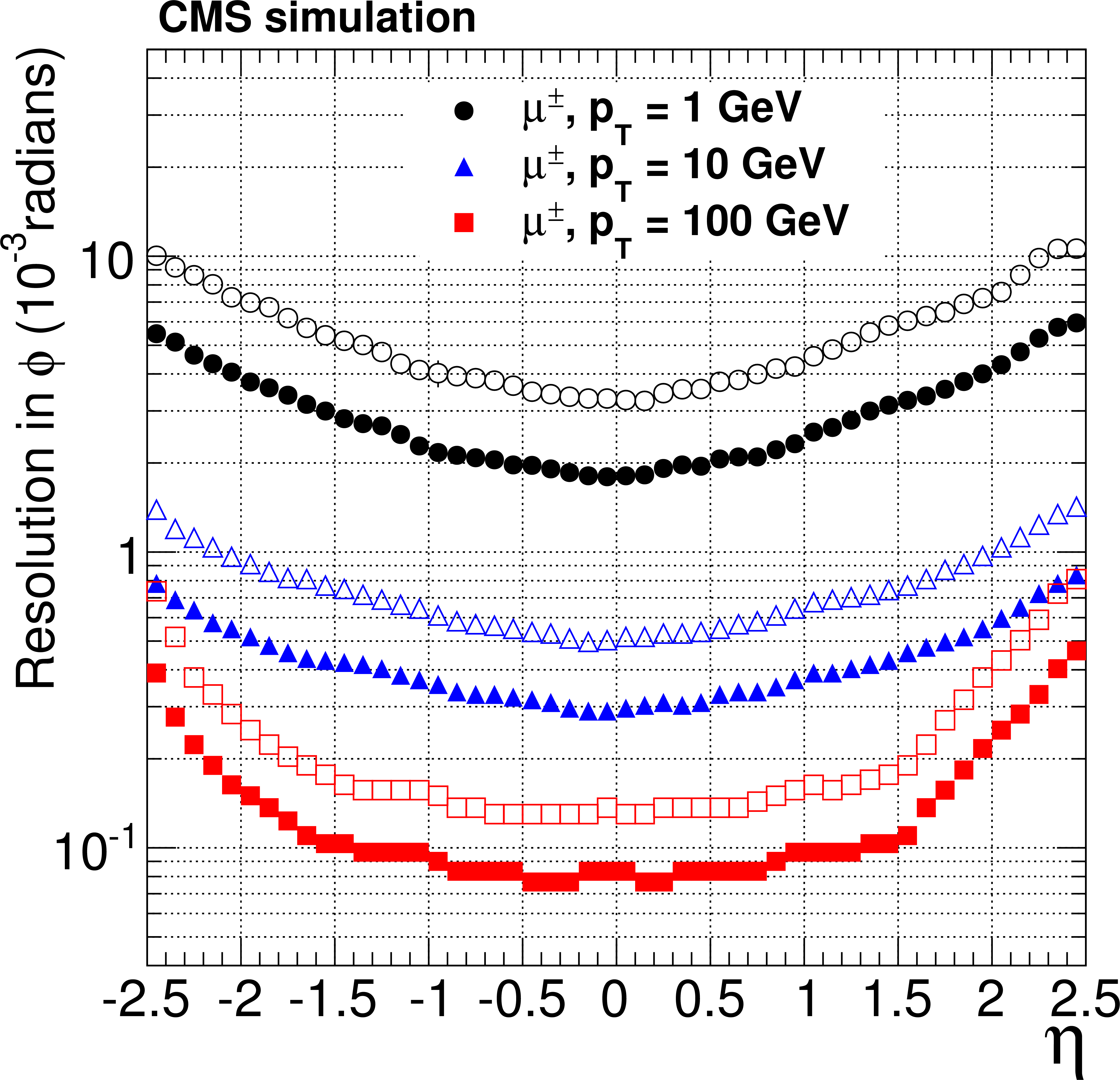
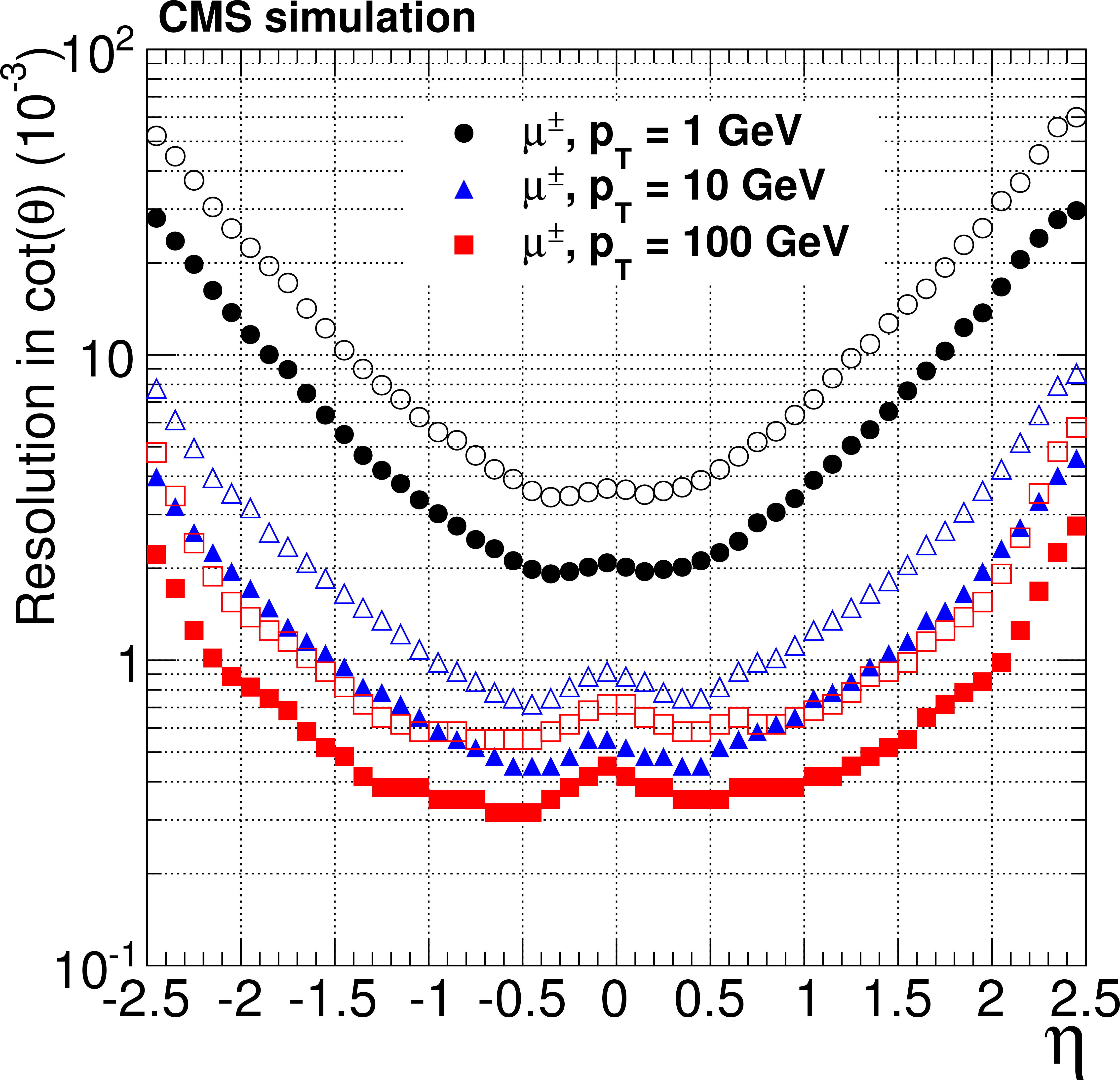
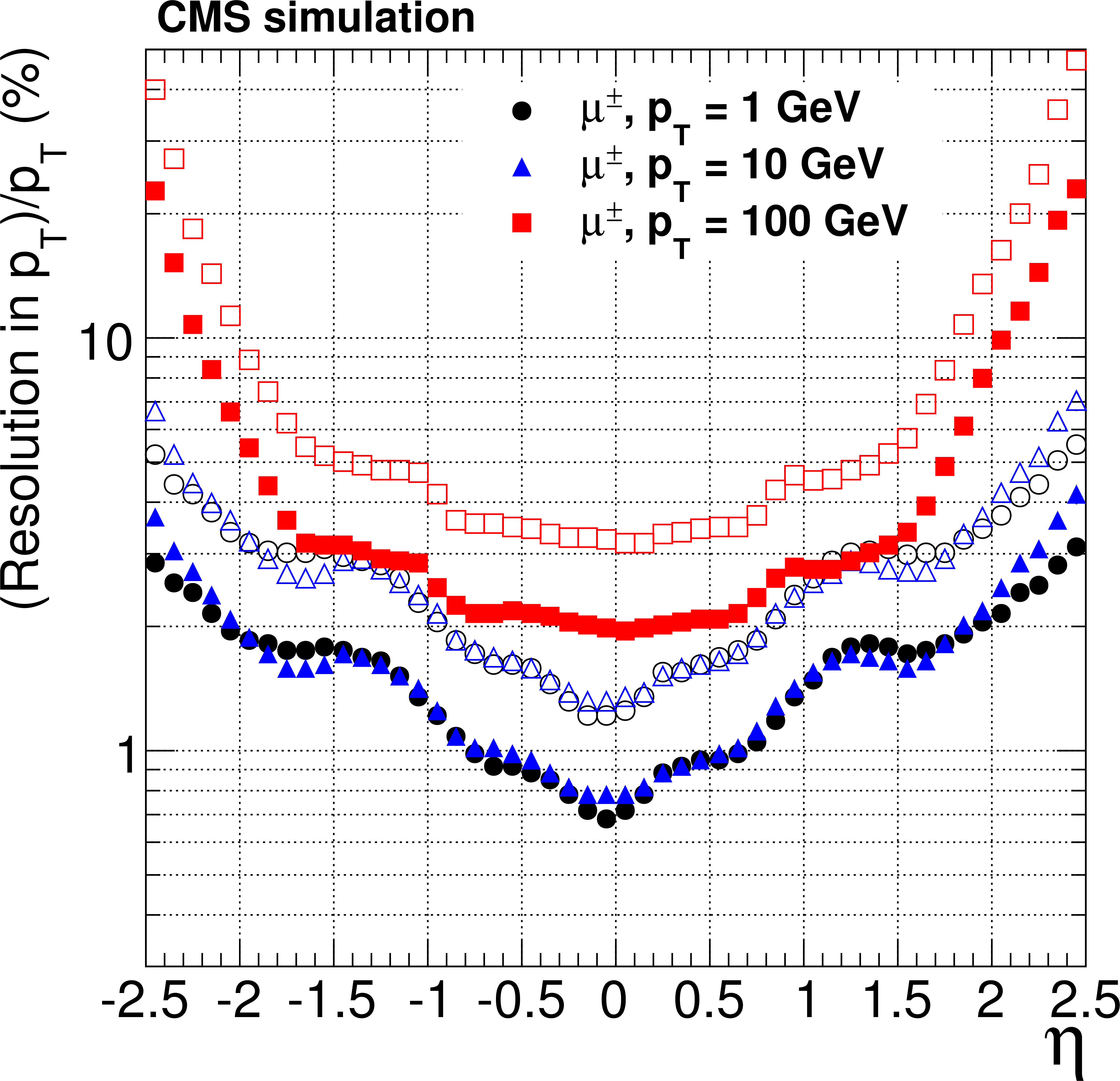
Figure 14-a:
Resolution, as a function of pseudorapidity, in the five track parameters for single, isolated muons with $ {p_{\mathrm {T}}} =$ 1, 10, and 100 GeV. From a to e: transverse and longitudinal impact parameters, $\phi $, $\mathrm{ cotan }\theta $ and transverse momentum. For each bin in $\eta $, the solid (open) symbols correspond to the half-width for 68% (90%) intervals centered on the mode of the distribution in residuals, as described in the text. |
png pdf |
Figure 14-b:
Resolution, as a function of pseudorapidity, in the five track parameters for single, isolated muons with $ {p_{\mathrm {T}}} =$ 1, 10, and 100 GeV. From a to e: transverse and longitudinal impact parameters, $\phi $, $\mathrm{ cotan }\theta $ and transverse momentum. For each bin in $\eta $, the solid (open) symbols correspond to the half-width for 68% (90%) intervals centered on the mode of the distribution in residuals, as described in the text. |
png pdf |
Figure 14-c:
Resolution, as a function of pseudorapidity, in the five track parameters for single, isolated muons with $ {p_{\mathrm {T}}} =$ 1, 10, and 100 GeV. From a to e: transverse and longitudinal impact parameters, $\phi $, $\mathrm{ cotan }\theta $ and transverse momentum. For each bin in $\eta $, the solid (open) symbols correspond to the half-width for 68% (90%) intervals centered on the mode of the distribution in residuals, as described in the text. |
png pdf |
Figure 14-d:
Resolution, as a function of pseudorapidity, in the five track parameters for single, isolated muons with $ {p_{\mathrm {T}}} =$ 1, 10, and 100 GeV. From a to e: transverse and longitudinal impact parameters, $\phi $, $\mathrm{ cotan }\theta $ and transverse momentum. For each bin in $\eta $, the solid (open) symbols correspond to the half-width for 68% (90%) intervals centered on the mode of the distribution in residuals, as described in the text. |
png pdf |
Figure 14-e:
Resolution, as a function of pseudorapidity, in the five track parameters for single, isolated muons with $ {p_{\mathrm {T}}} =$ 1, 10, and 100 GeV. From a to e: transverse and longitudinal impact parameters, $\phi $, $\mathrm{ cotan }\theta $ and transverse momentum. For each bin in $\eta $, the solid (open) symbols correspond to the half-width for 68% (90%) intervals centered on the mode of the distribution in residuals, as described in the text. |
png pdf |
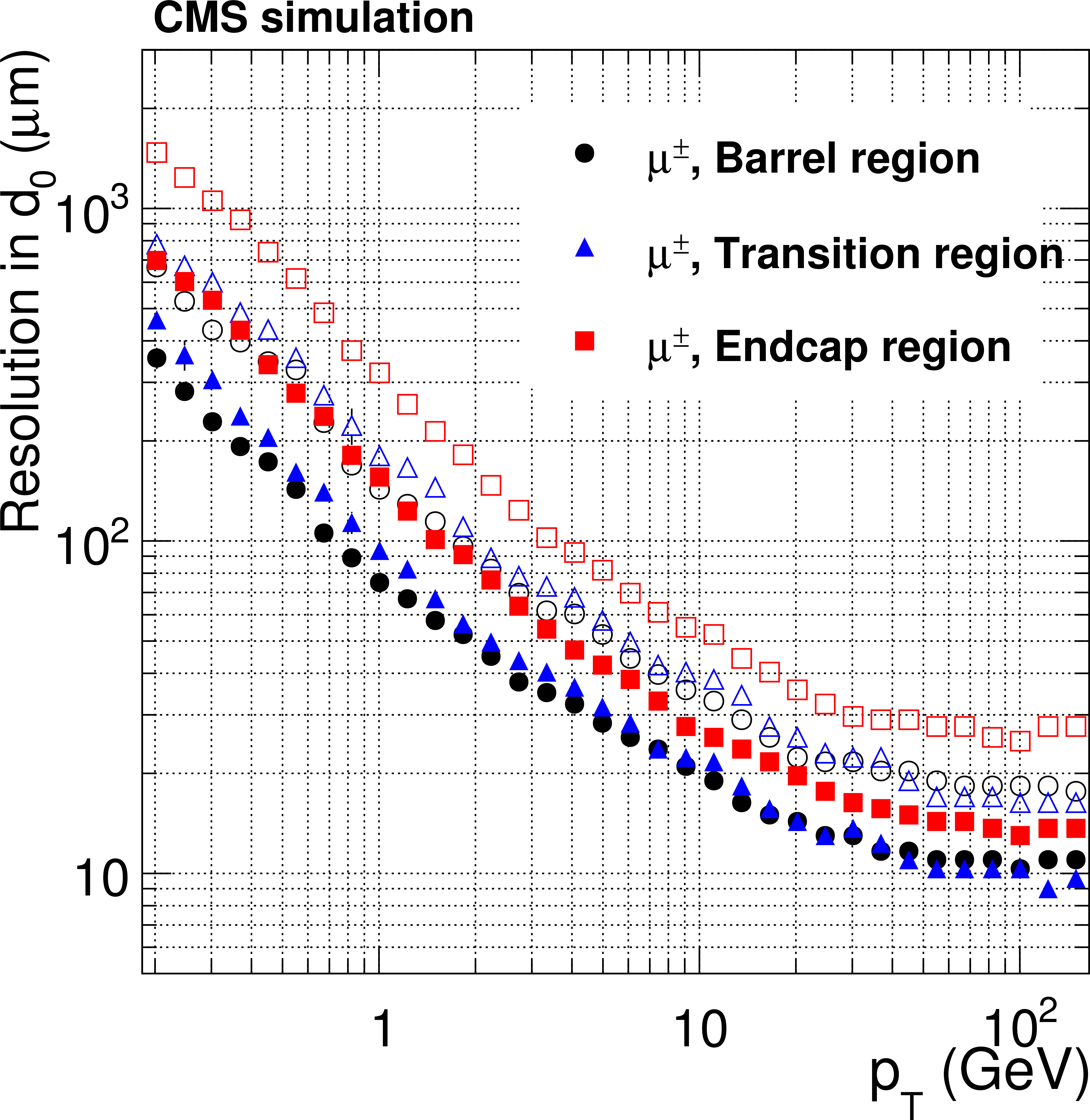
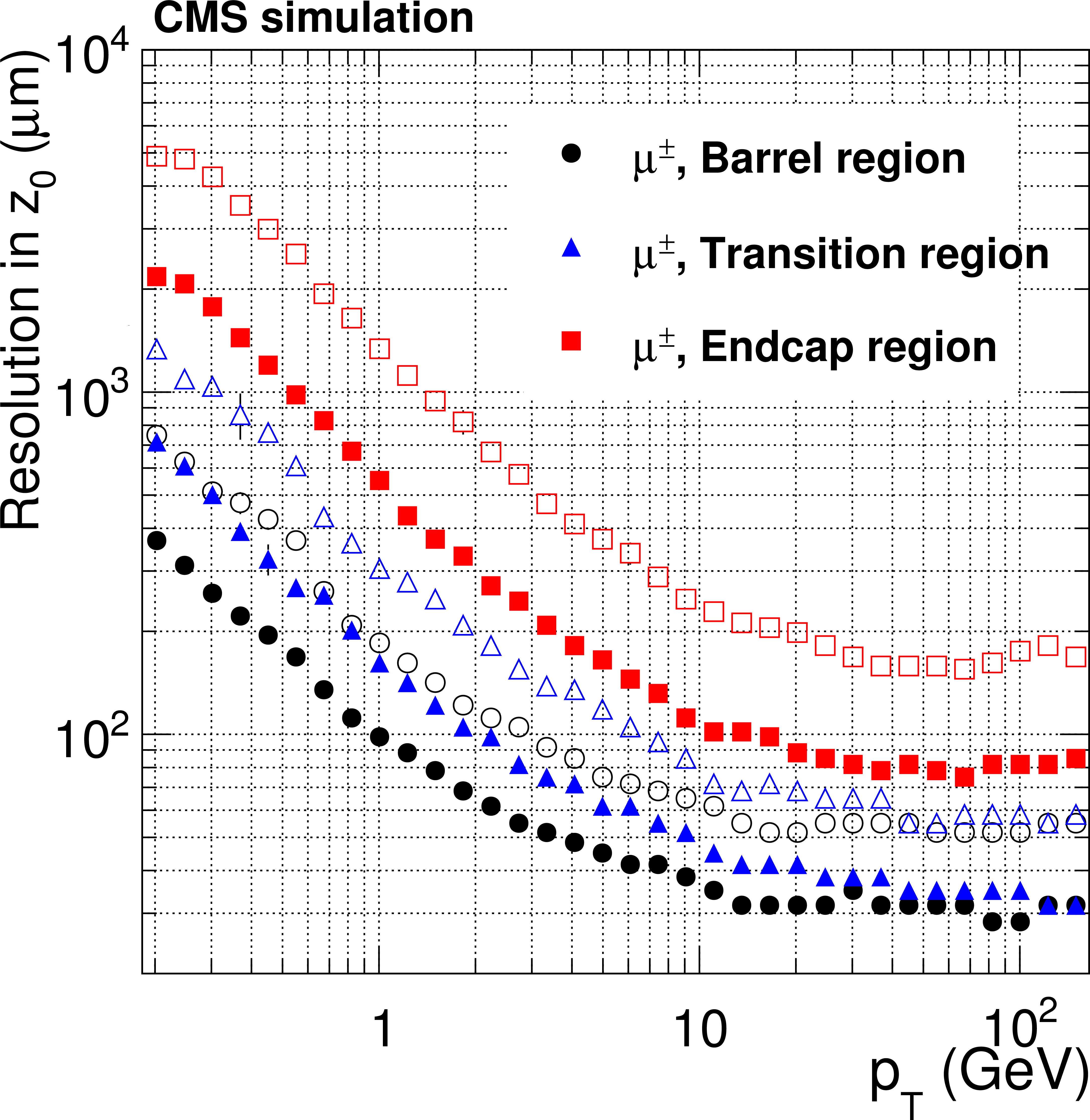
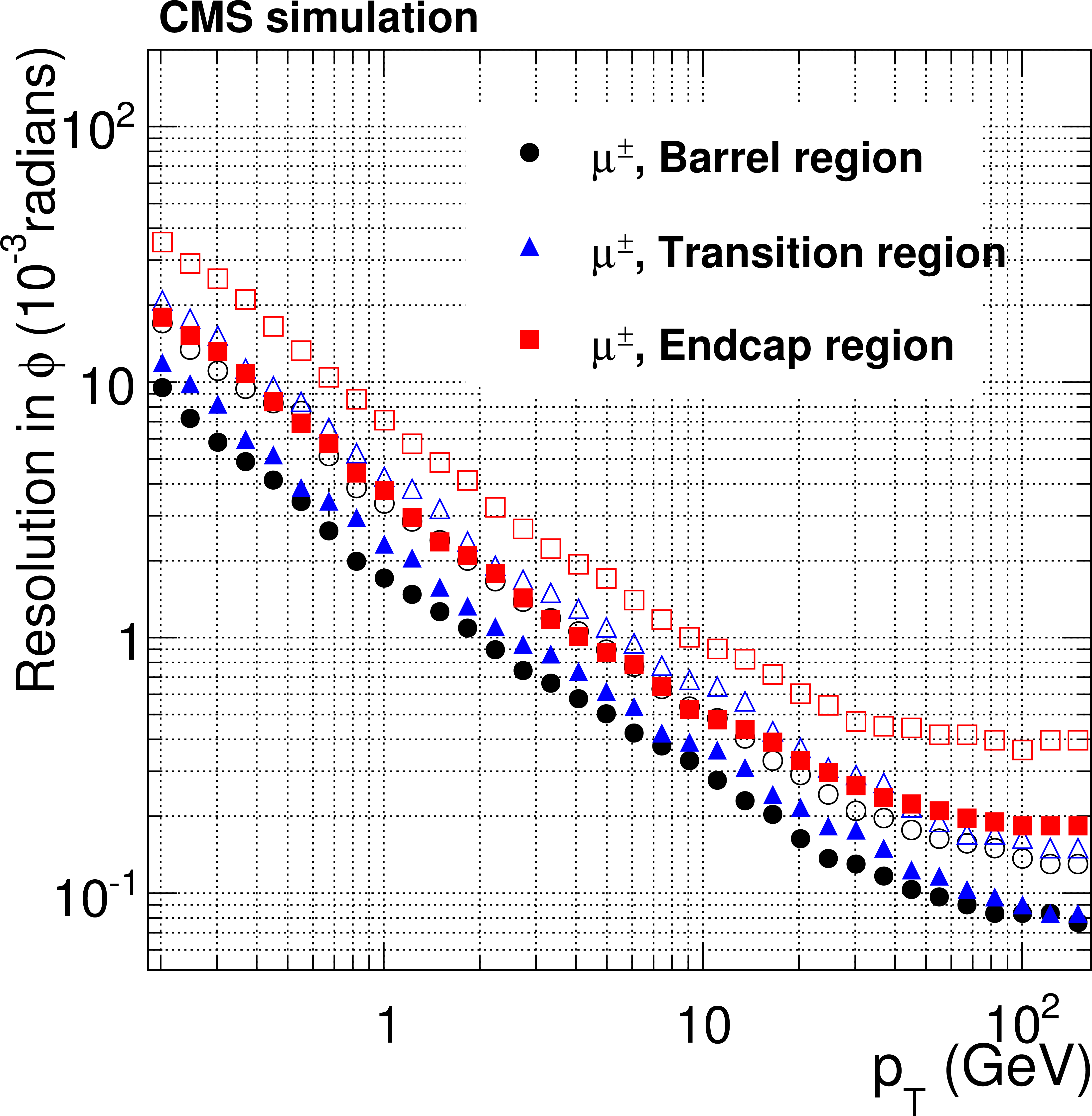
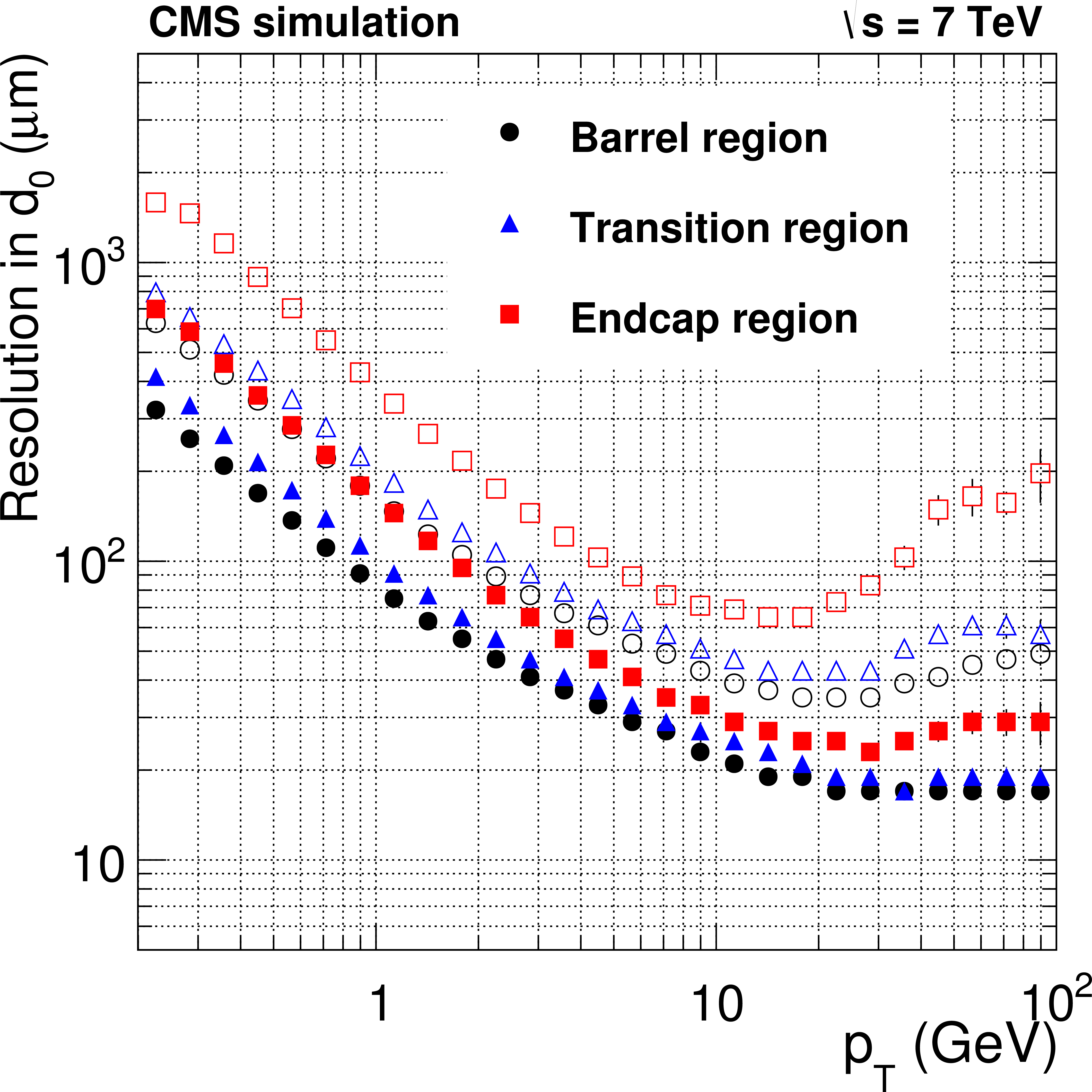
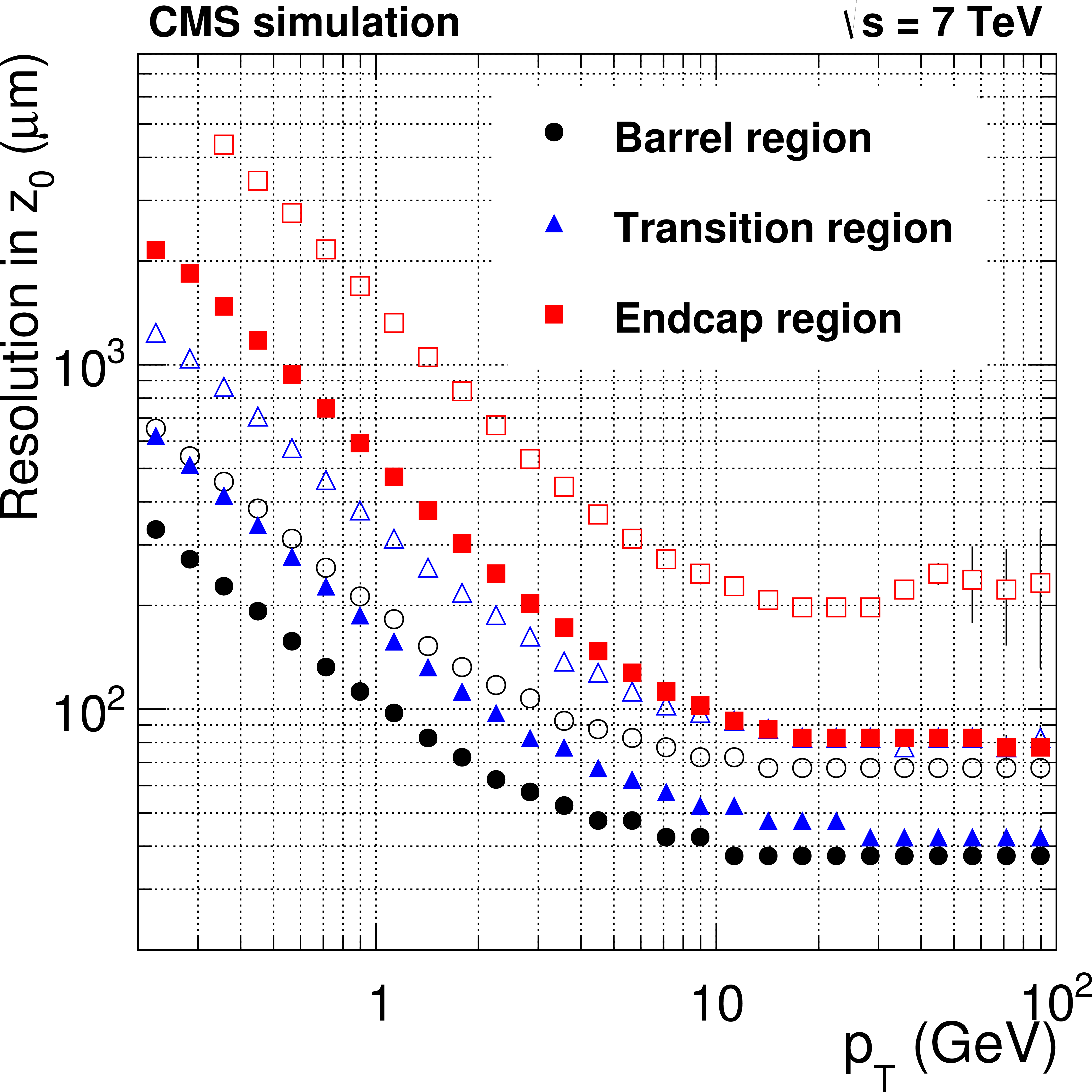
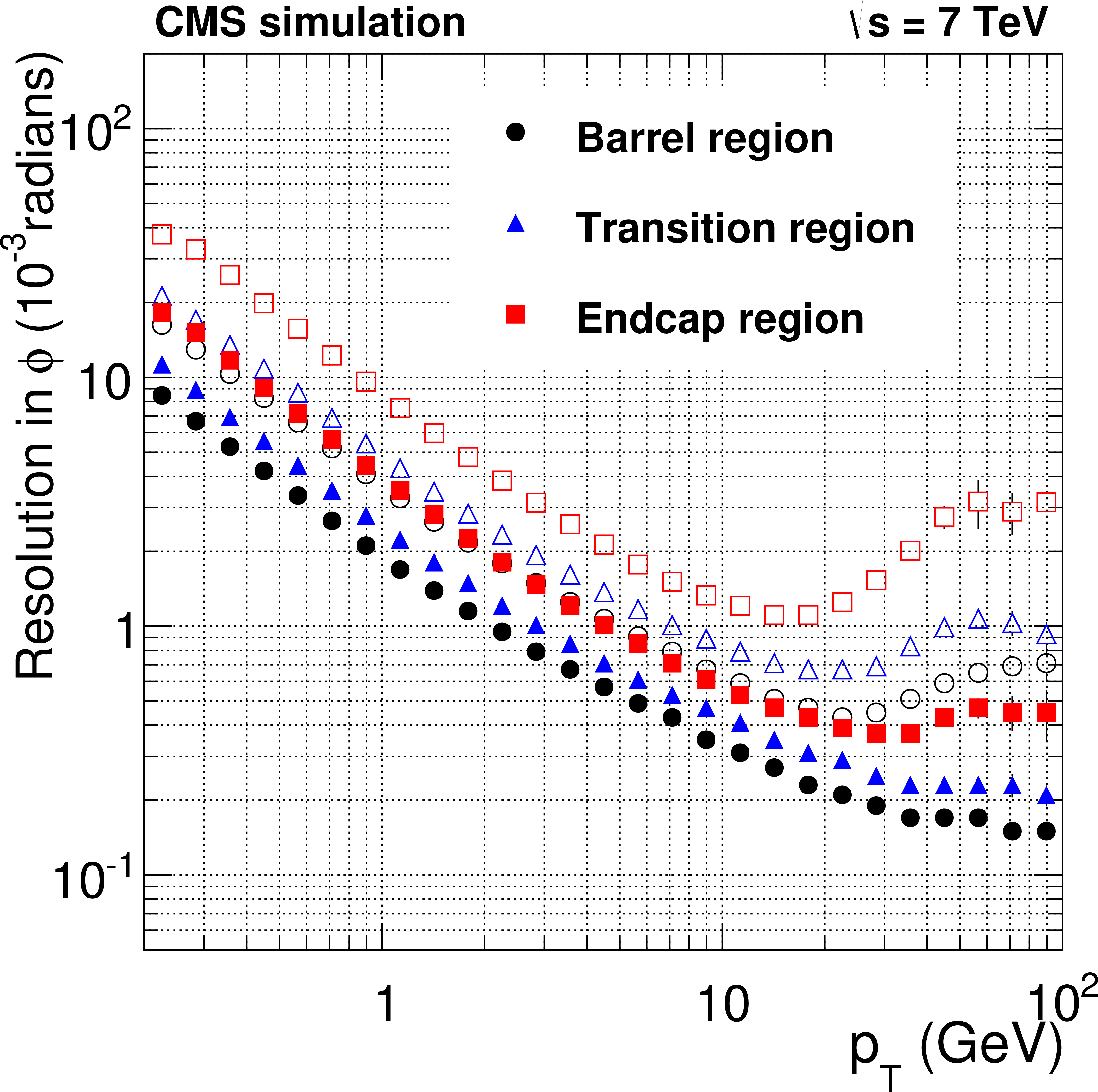
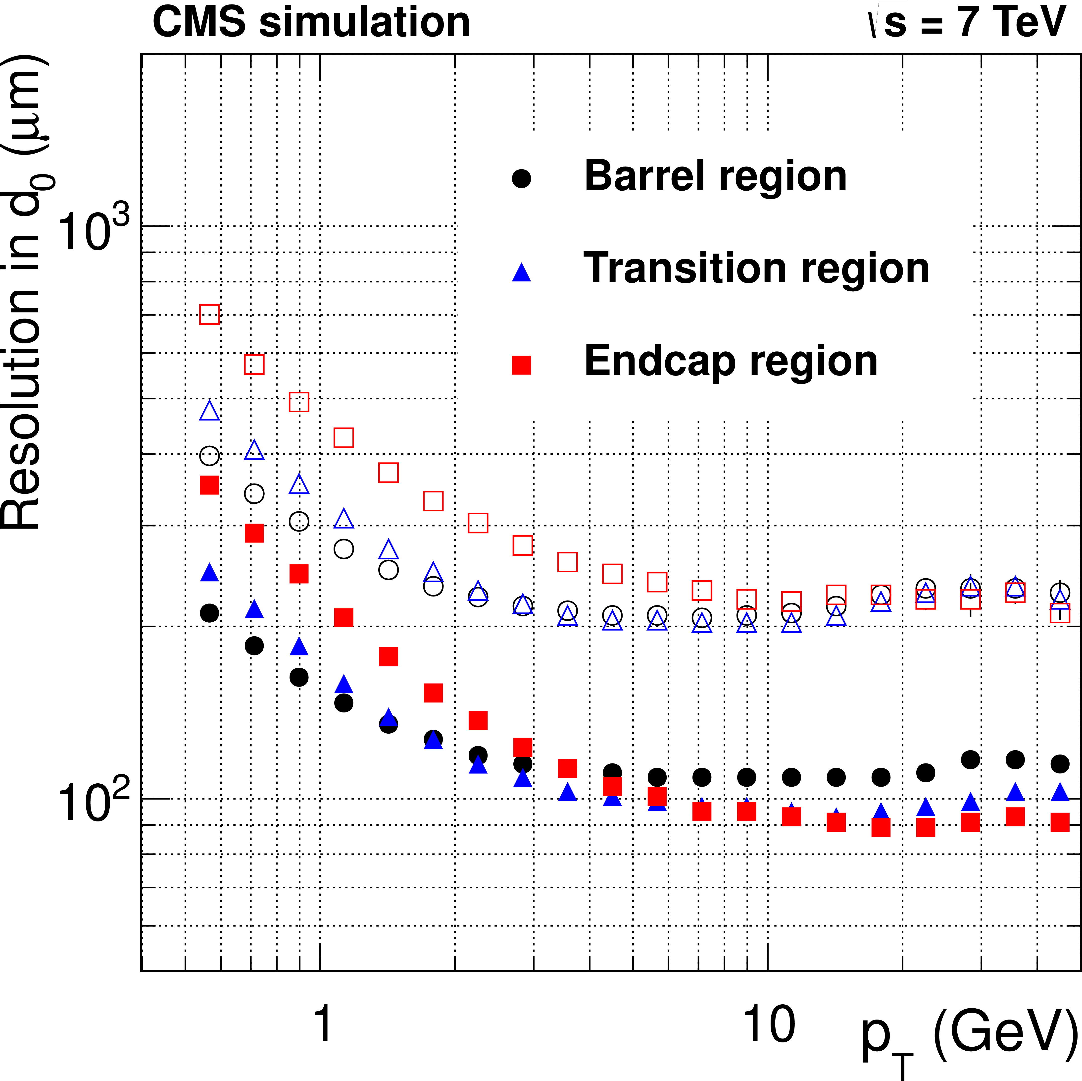
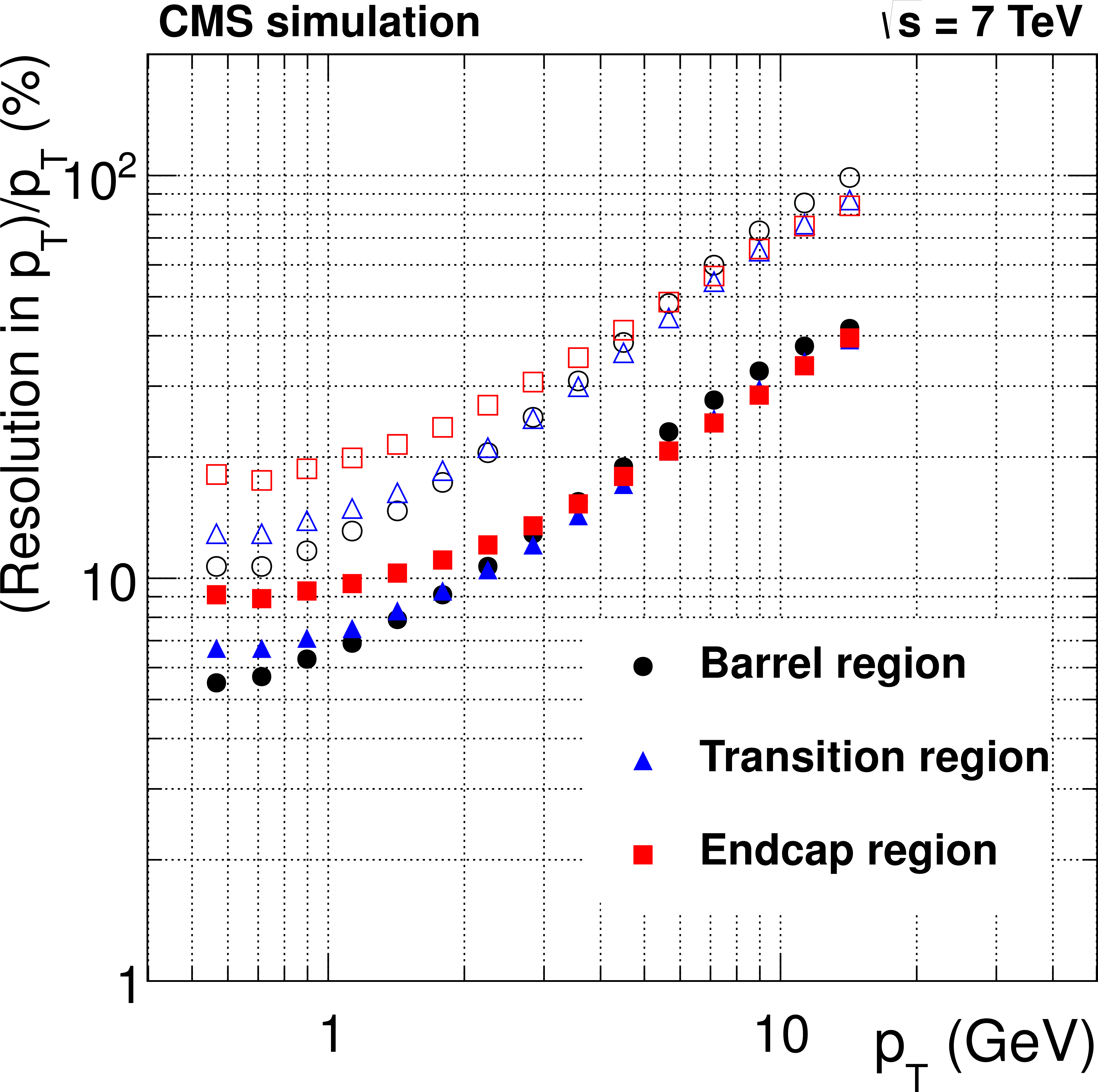
Figure 15-a:
Resolution, as a function of $ {p_{\mathrm {T}}} $, in the five track parameters for single, isolated muons in the barrel, transition, and endcap regions, defined by $\eta $ intervals of 0-0.9, 0.9-1.4 and 1.4-2.5, respectively. From a to e: transverse and longitudinal impact parameters, $\phi $, $\mathrm{ cotan }\theta $ and $ {p_{\mathrm {T}}} $. For each bin in $ {p_{\mathrm {T}}} $, the solid (open) symbols correspond to the half-width for 68% (90%) intervals centered on the mode of the distribution in residuals, as described in the text. |
png pdf |
Figure 15-b:
Resolution, as a function of $ {p_{\mathrm {T}}} $, in the five track parameters for single, isolated muons in the barrel, transition, and endcap regions, defined by $\eta $ intervals of 0-0.9, 0.9-1.4 and 1.4-2.5, respectively. From a to e: transverse and longitudinal impact parameters, $\phi $, $\mathrm{ cotan }\theta $ and $ {p_{\mathrm {T}}} $. For each bin in $ {p_{\mathrm {T}}} $, the solid (open) symbols correspond to the half-width for 68% (90%) intervals centered on the mode of the distribution in residuals, as described in the text. |
png pdf |
Figure 15-c:
Resolution, as a function of $ {p_{\mathrm {T}}} $, in the five track parameters for single, isolated muons in the barrel, transition, and endcap regions, defined by $\eta $ intervals of 0-0.9, 0.9-1.4 and 1.4-2.5, respectively. From a to e: transverse and longitudinal impact parameters, $\phi $, $\mathrm{ cotan }\theta $ and $ {p_{\mathrm {T}}} $. For each bin in $ {p_{\mathrm {T}}} $, the solid (open) symbols correspond to the half-width for 68% (90%) intervals centered on the mode of the distribution in residuals, as described in the text. |
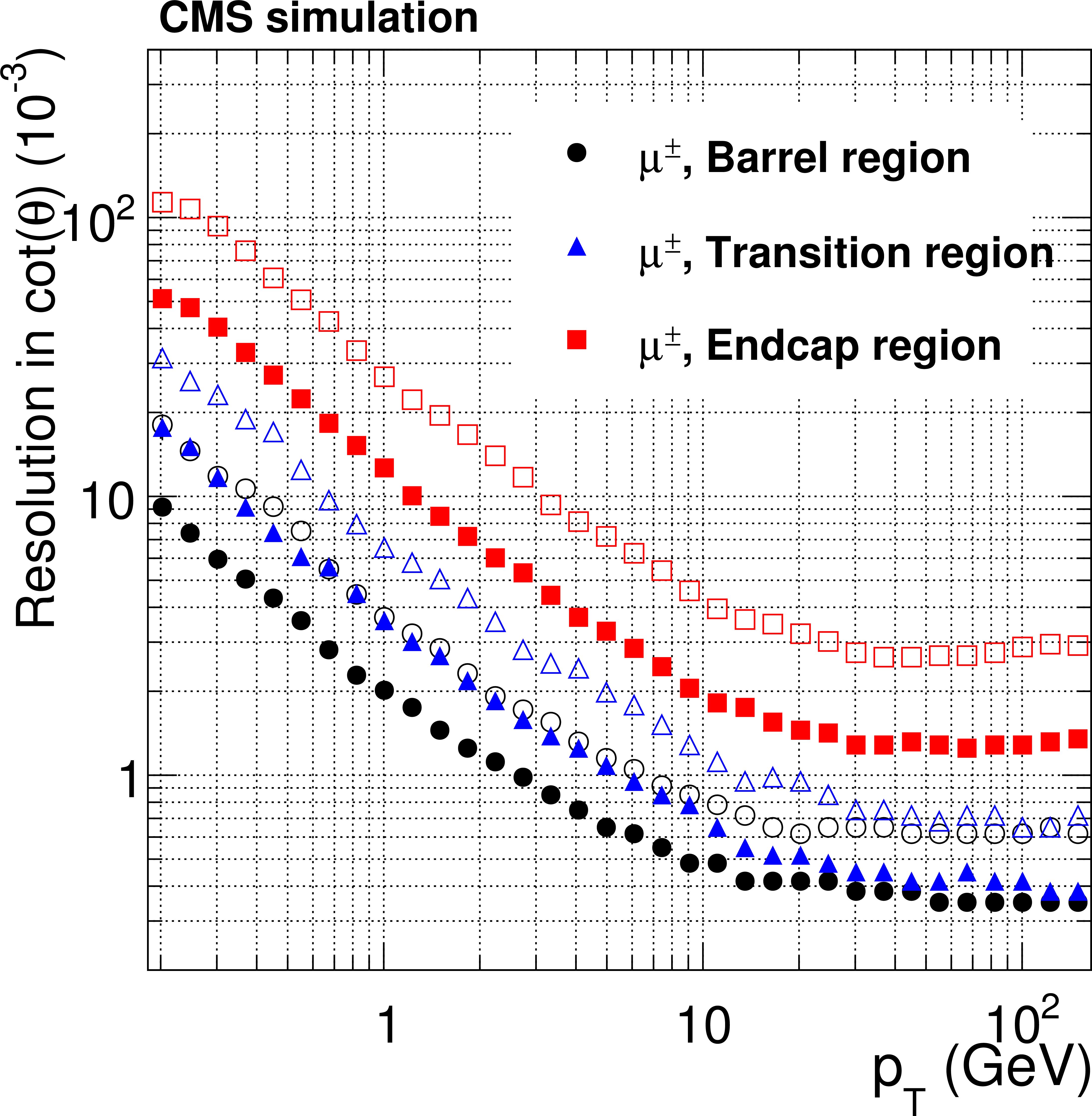
png pdf |
Figure 15-d:
Resolution, as a function of $ {p_{\mathrm {T}}} $, in the five track parameters for single, isolated muons in the barrel, transition, and endcap regions, defined by $\eta $ intervals of 0-0.9, 0.9-1.4 and 1.4-2.5, respectively. From a to e: transverse and longitudinal impact parameters, $\phi $, $\mathrm{ cotan }\theta $ and $ {p_{\mathrm {T}}} $. For each bin in $ {p_{\mathrm {T}}} $, the solid (open) symbols correspond to the half-width for 68% (90%) intervals centered on the mode of the distribution in residuals, as described in the text. |
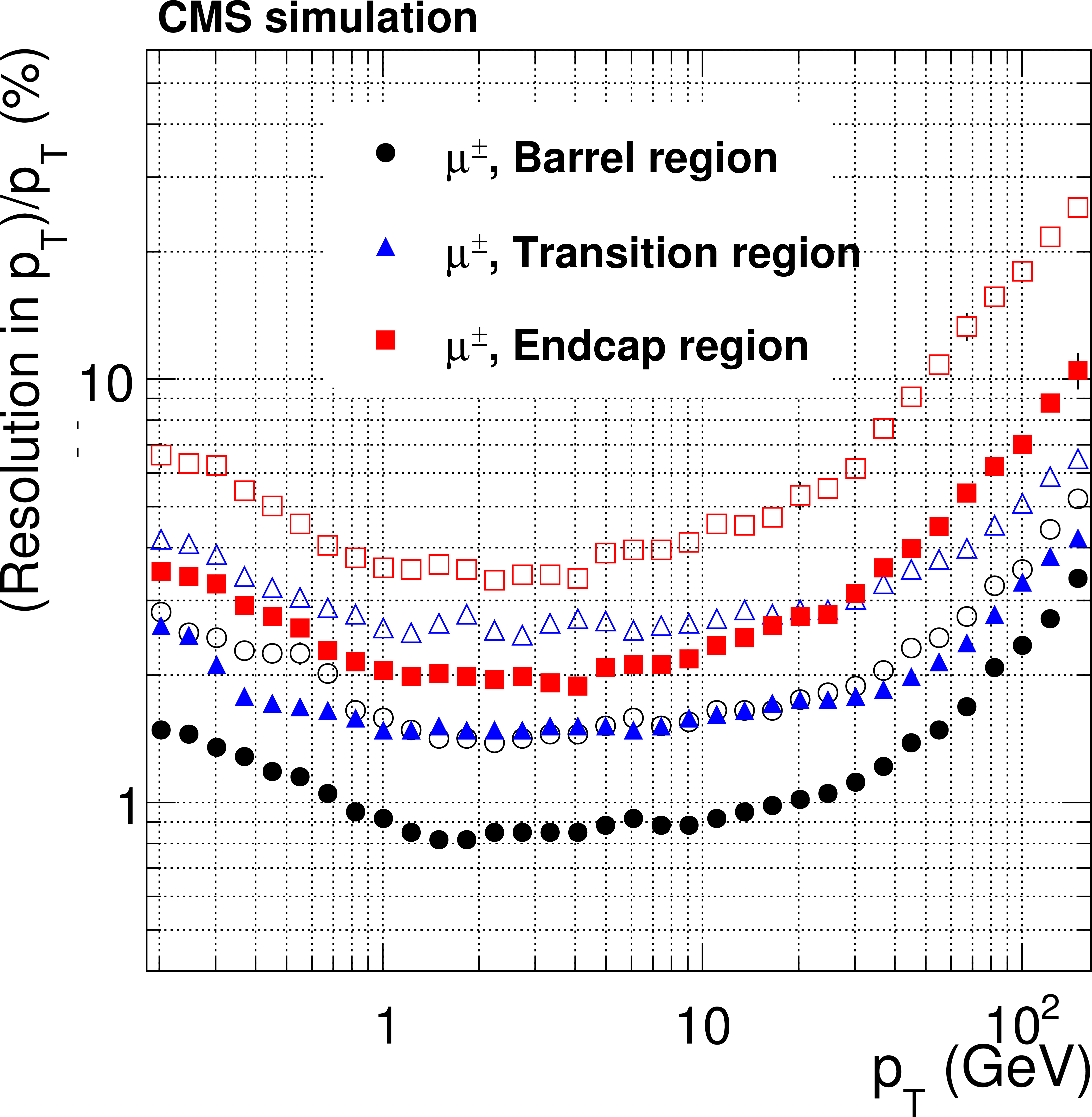
png pdf |
Figure 15-e:
Resolution, as a function of $ {p_{\mathrm {T}}} $, in the five track parameters for single, isolated muons in the barrel, transition, and endcap regions, defined by $\eta $ intervals of 0-0.9, 0.9-1.4 and 1.4-2.5, respectively. From a to e: transverse and longitudinal impact parameters, $\phi $, $\mathrm{ cotan }\theta $ and $ {p_{\mathrm {T}}} $. For each bin in $ {p_{\mathrm {T}}} $, the solid (open) symbols correspond to the half-width for 68% (90%) intervals centered on the mode of the distribution in residuals, as described in the text. |
png pdf |
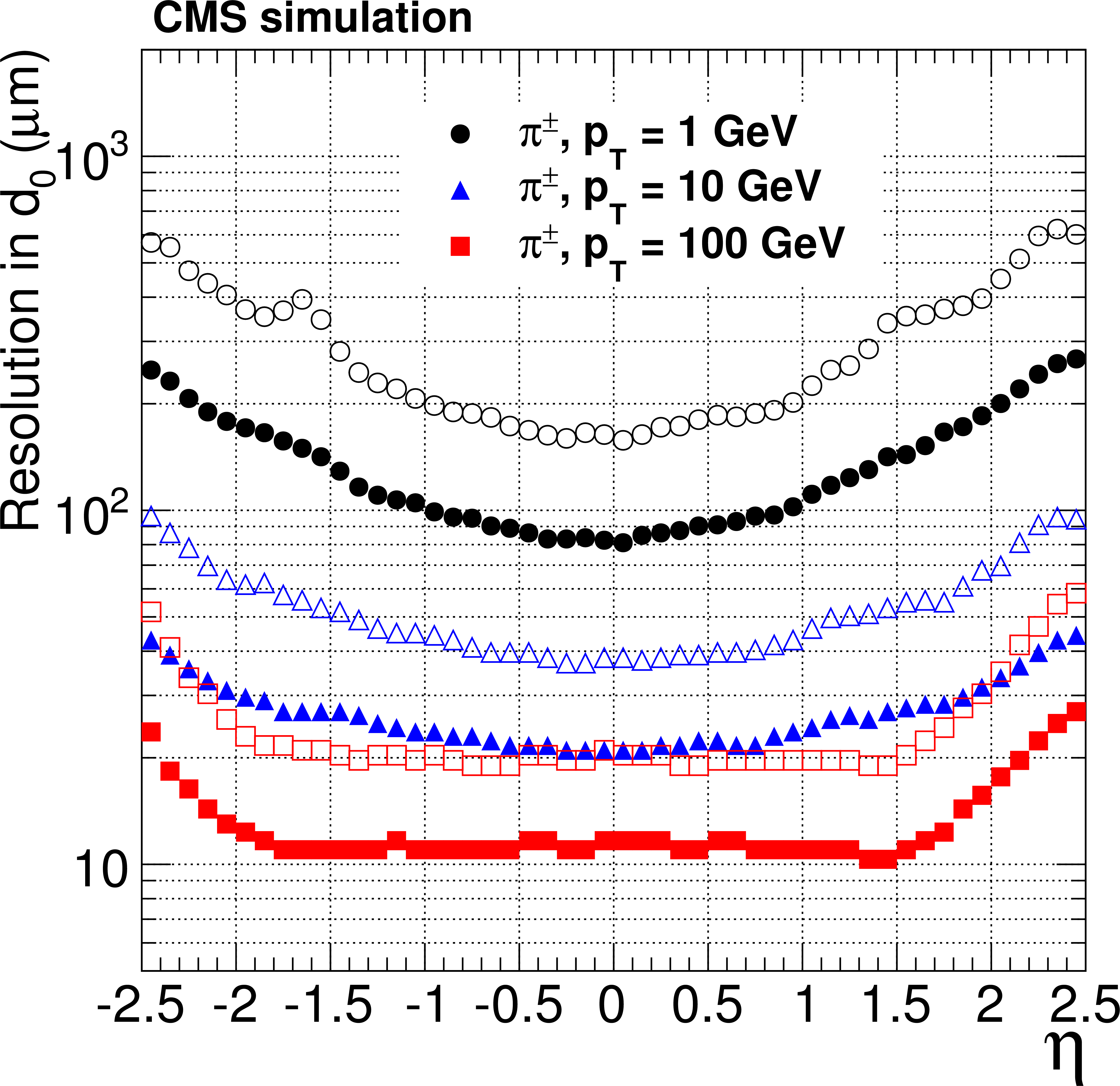
Figure 16-a:
Resolution, as a function of pseudorapidity, in the five track parameters for single, isolated pions with transverse momenta of 1, 10, and 100 GeV. From a to e: transverse and longitudinal impact parameters, $\phi $, $\mathrm{ cotan }\theta $ and $ {p_{\mathrm {T}}} $ . For each bin in $\eta $, the solid (open) symbols correspond to the half-width for 68% (90%) intervals centered on the mode of the distribution in residuals, as described in the text. |
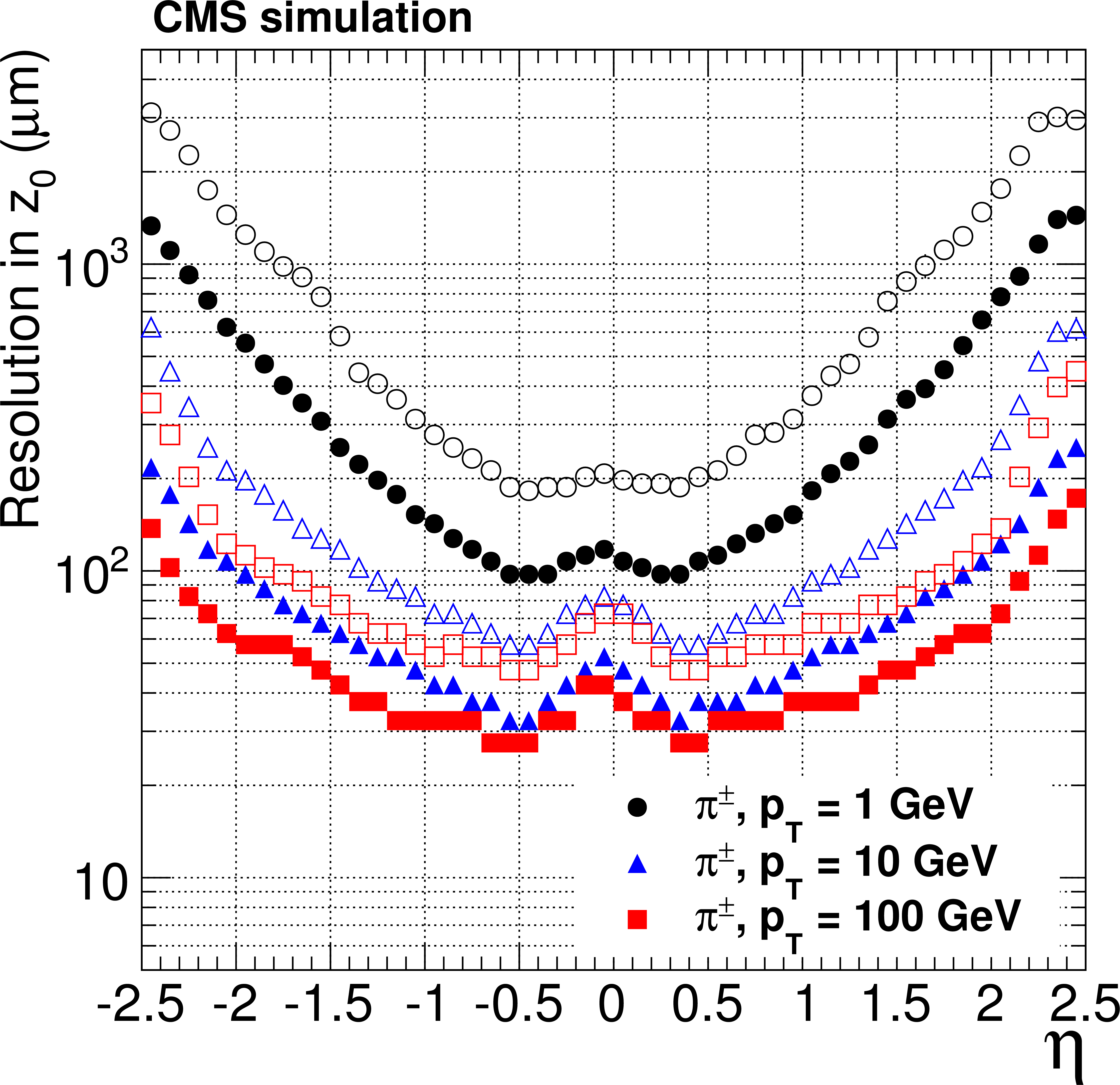
png pdf |
Figure 16-b:
Resolution, as a function of pseudorapidity, in the five track parameters for single, isolated pions with transverse momenta of 1, 10, and 100 GeV. From a to e: transverse and longitudinal impact parameters, $\phi $, $\mathrm{ cotan }\theta $ and $ {p_{\mathrm {T}}} $ . For each bin in $\eta $, the solid (open) symbols correspond to the half-width for 68% (90%) intervals centered on the mode of the distribution in residuals, as described in the text. |
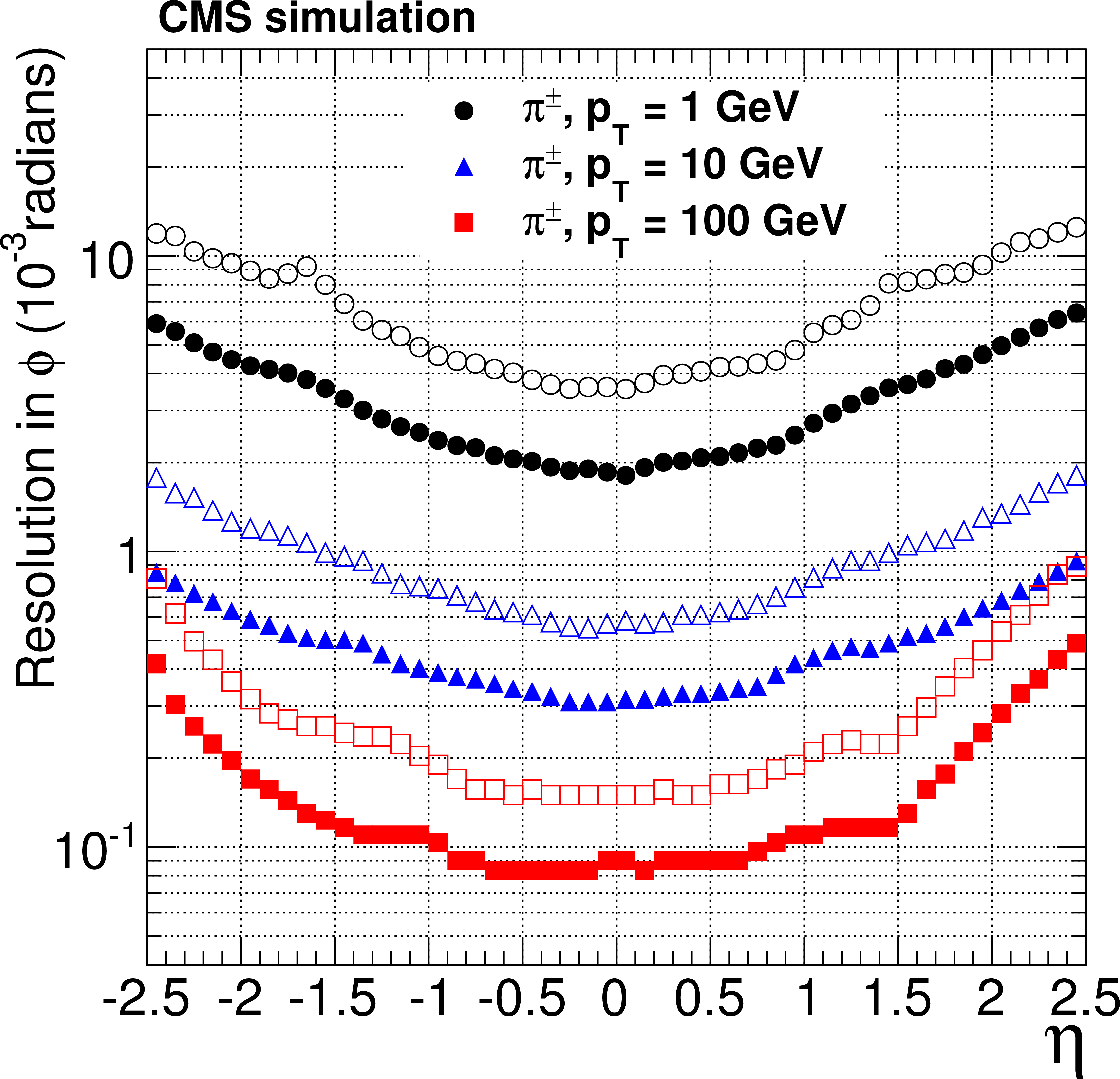
png pdf |
Figure 16-c:
Resolution, as a function of pseudorapidity, in the five track parameters for single, isolated pions with transverse momenta of 1, 10, and 100 GeV. From a to e: transverse and longitudinal impact parameters, $\phi $, $\mathrm{ cotan }\theta $ and $ {p_{\mathrm {T}}} $ . For each bin in $\eta $, the solid (open) symbols correspond to the half-width for 68% (90%) intervals centered on the mode of the distribution in residuals, as described in the text. |

png pdf |
Figure 16-d:
Resolution, as a function of pseudorapidity, in the five track parameters for single, isolated pions with transverse momenta of 1, 10, and 100 GeV. From a to e: transverse and longitudinal impact parameters, $\phi $, $\mathrm{ cotan }\theta $ and $ {p_{\mathrm {T}}} $ . For each bin in $\eta $, the solid (open) symbols correspond to the half-width for 68% (90%) intervals centered on the mode of the distribution in residuals, as described in the text. |

png pdf |
Figure 16-e:
Resolution, as a function of pseudorapidity, in the five track parameters for single, isolated pions with transverse momenta of 1, 10, and 100 GeV. From a to e: transverse and longitudinal impact parameters, $\phi $, $\mathrm{ cotan }\theta $ and $ {p_{\mathrm {T}}} $ . For each bin in $\eta $, the solid (open) symbols correspond to the half-width for 68% (90%) intervals centered on the mode of the distribution in residuals, as described in the text. |
png pdf |
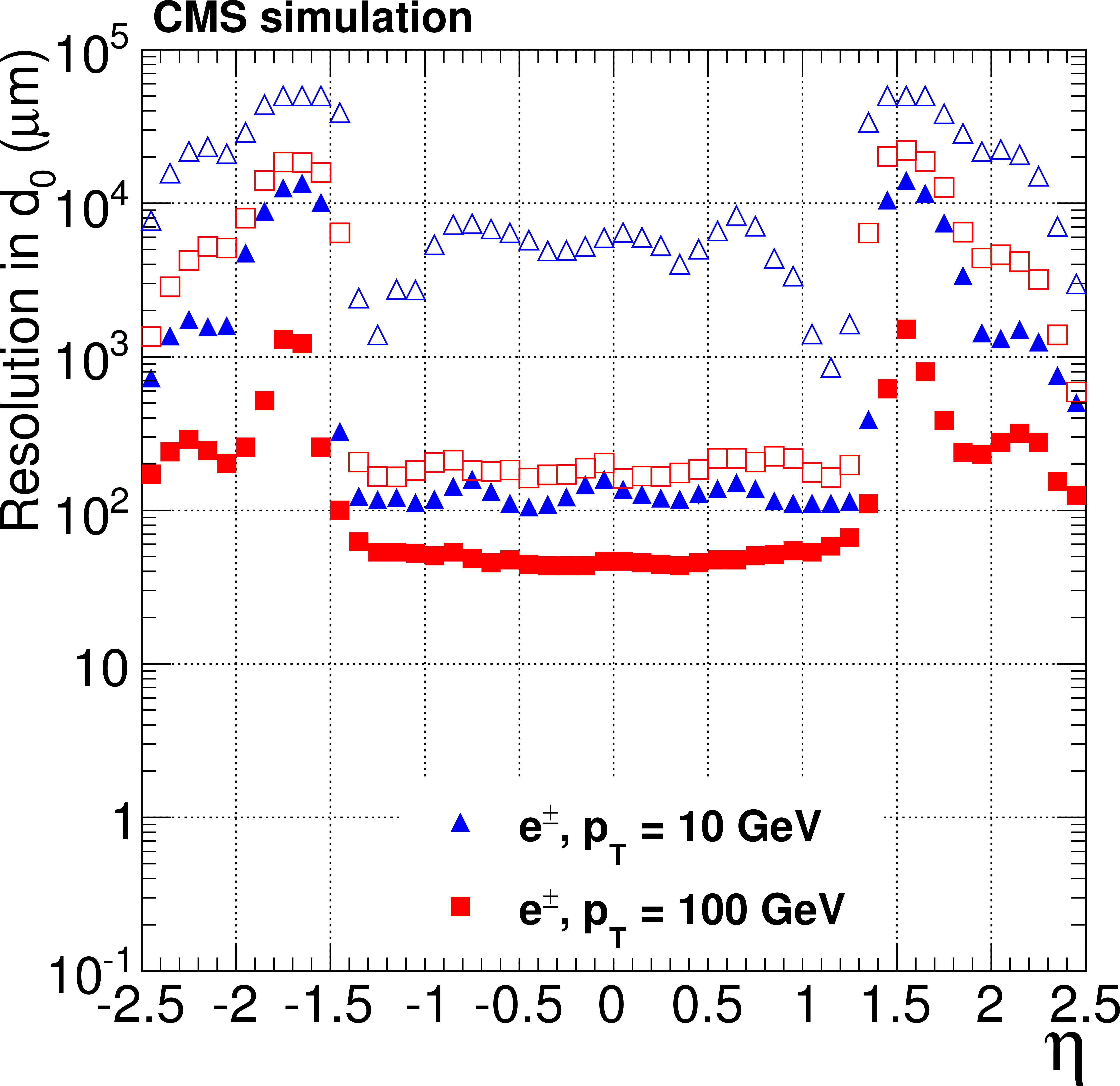
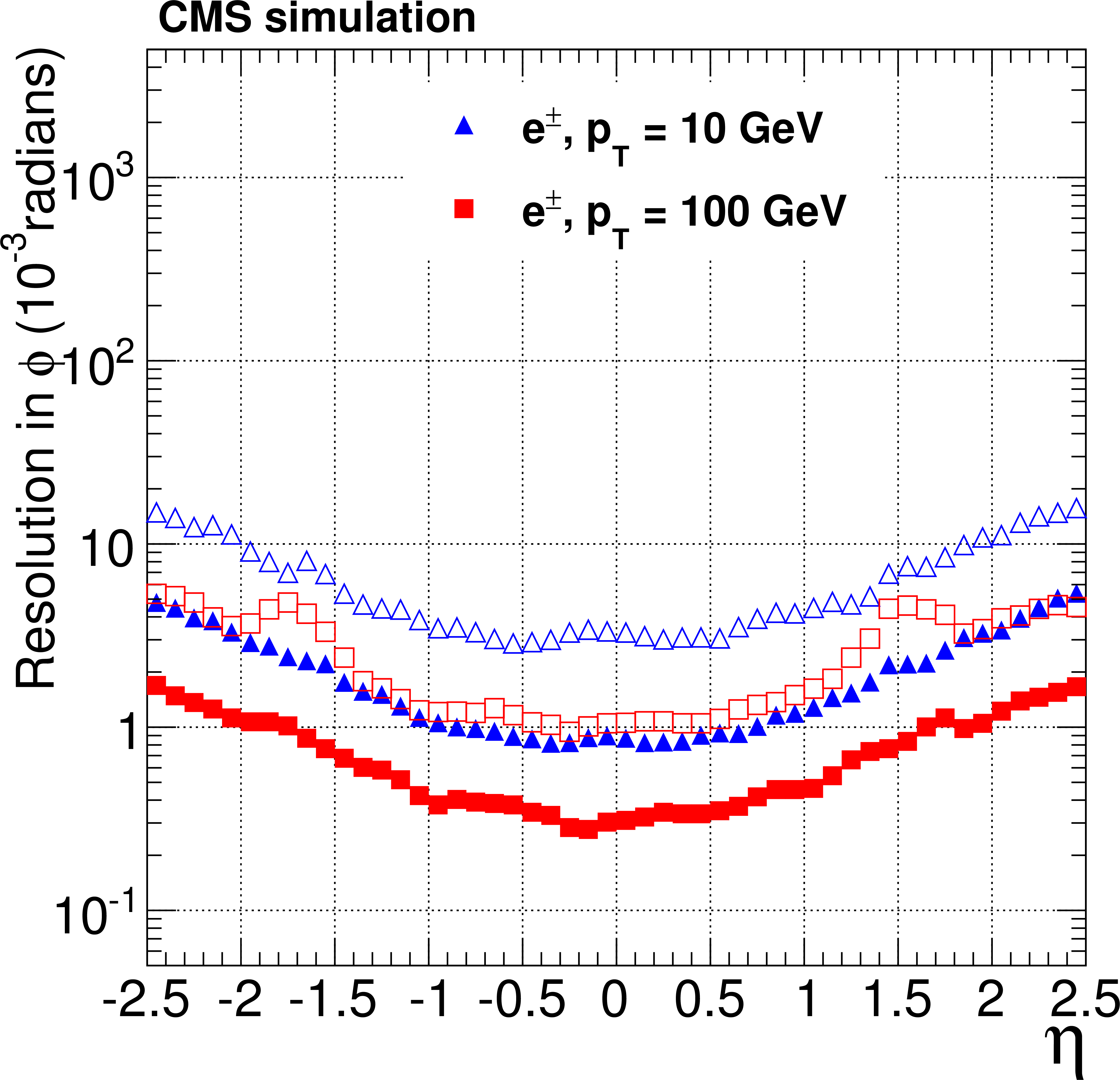
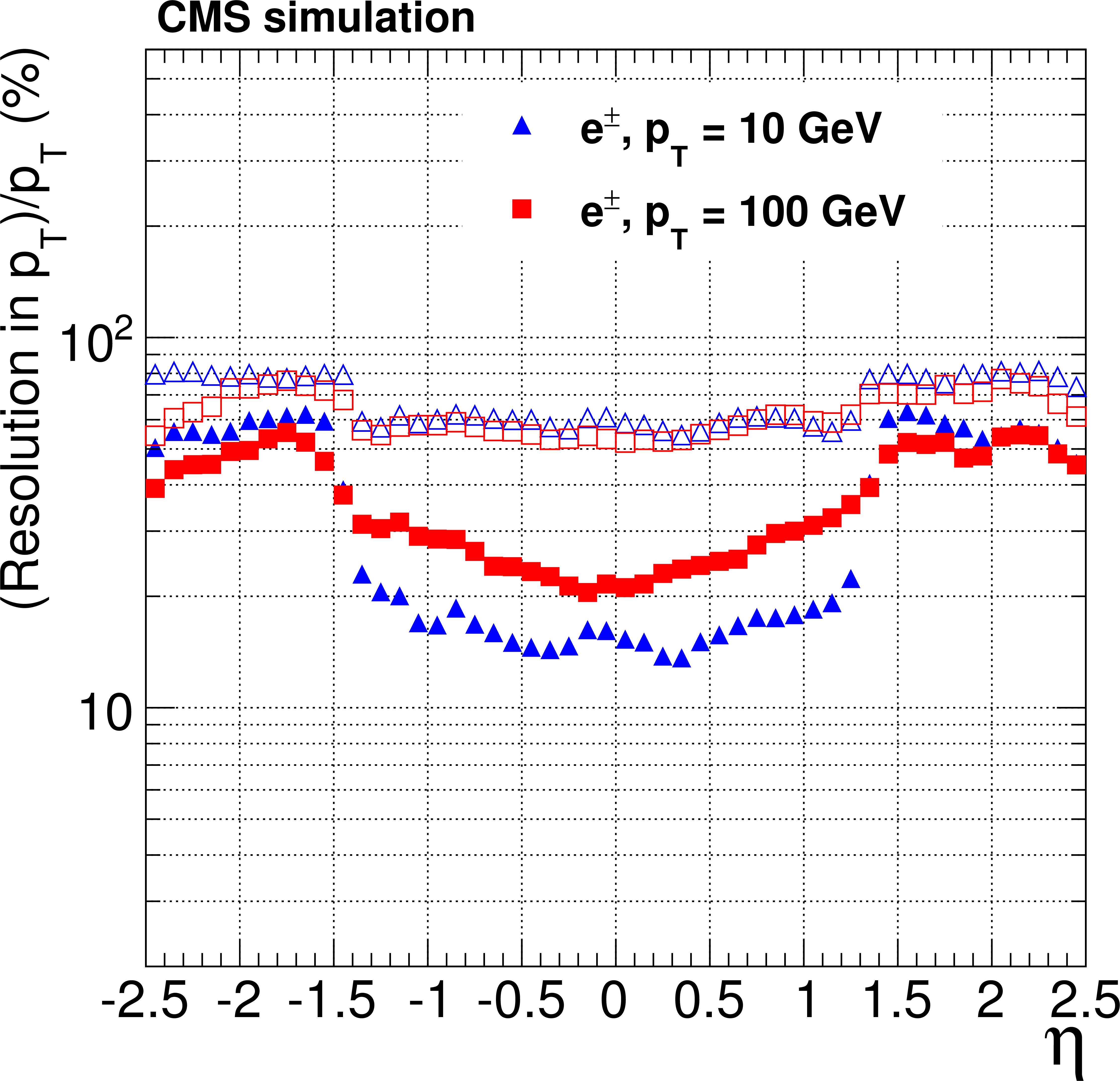
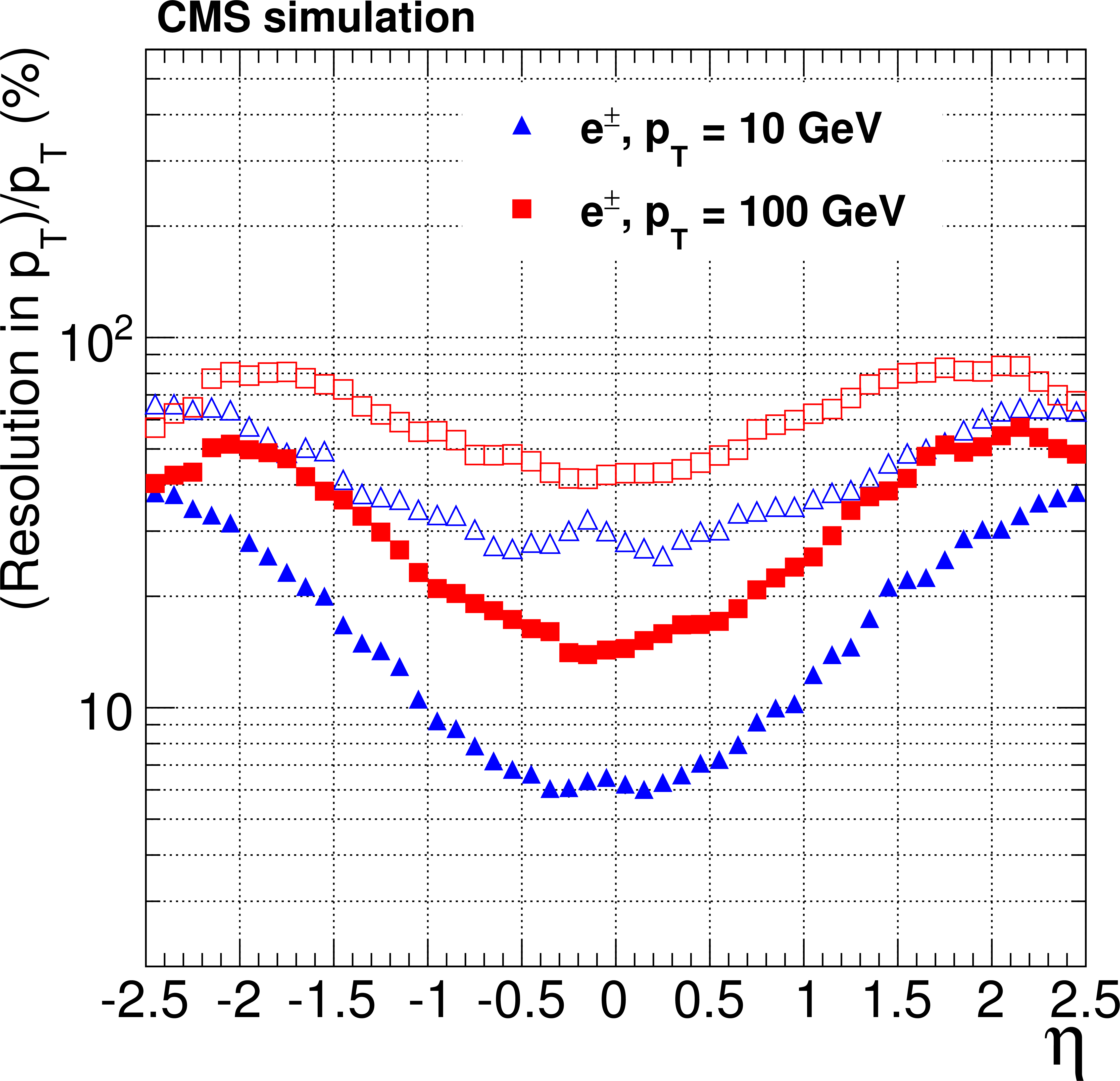
Figure 17-a:
Resolution, as a function of pseudorapidity, in the $d_0$, $\phi $ and $ {p_{\mathrm {T}}} $ track parameters for single, isolated electrons with $ {p_{\mathrm {T}}} = 10$ and 100 GeV. For each bin in $\eta $, the solid (open) symbols correspond to the width of the 68% (90%) intervals having its origin on the mode of the distribution in residuals, as described in the text. Only the half of the residuals distribution that does contain the non-Gaussian tail due to bremsstrahlung is considered in the interval calculation. The a, c, e (b, d, f) plots are of electrons reconstructed with the CTF (GSF) algorithm. |
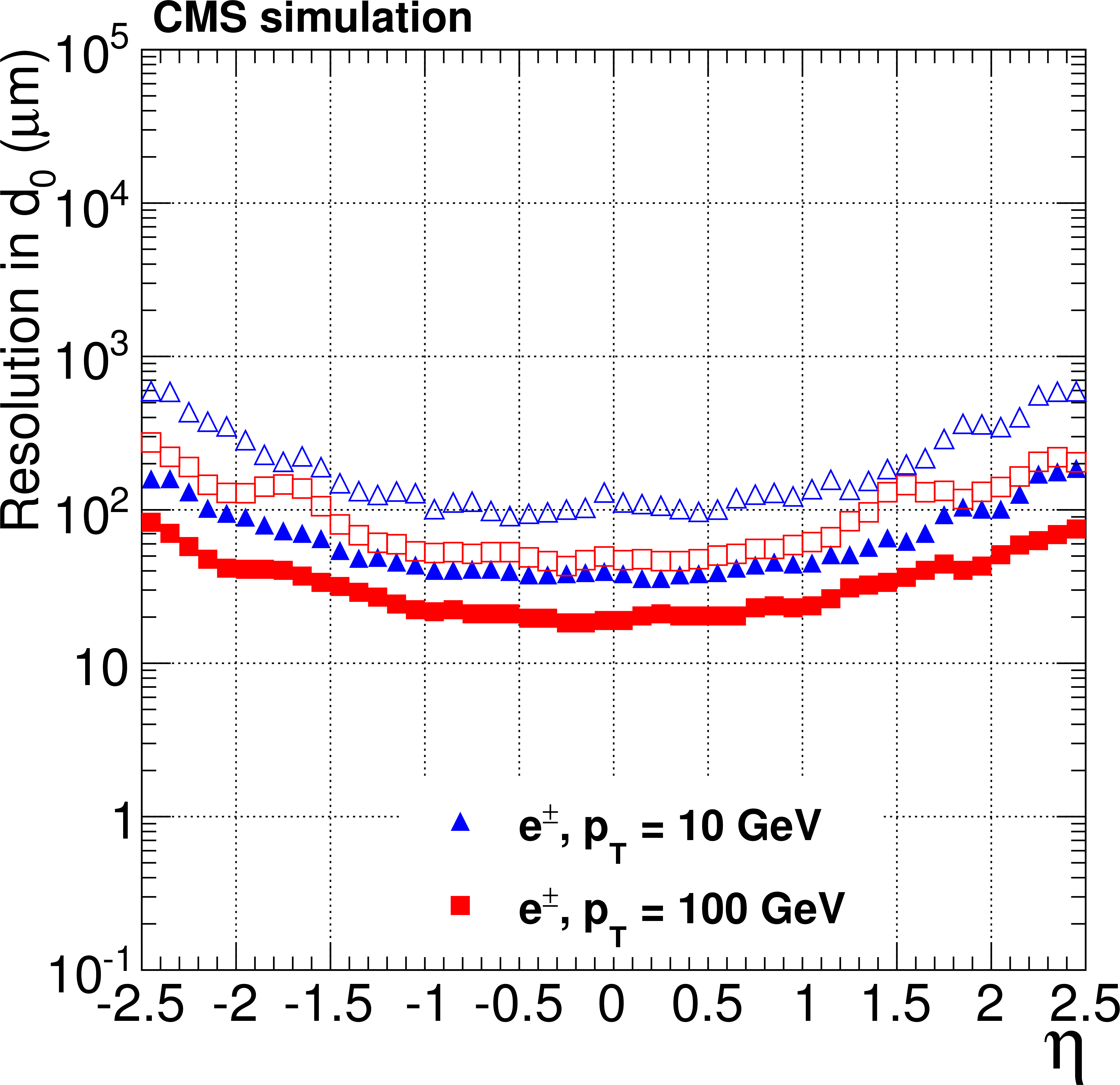
png pdf |
Figure 17-b:
Resolution, as a function of pseudorapidity, in the $d_0$, $\phi $ and $ {p_{\mathrm {T}}} $ track parameters for single, isolated electrons with $ {p_{\mathrm {T}}} = 10$ and 100 GeV. For each bin in $\eta $, the solid (open) symbols correspond to the width of the 68% (90%) intervals having its origin on the mode of the distribution in residuals, as described in the text. Only the half of the residuals distribution that does contain the non-Gaussian tail due to bremsstrahlung is considered in the interval calculation. The a, c, e (b, d, f) plots are of electrons reconstructed with the CTF (GSF) algorithm. |
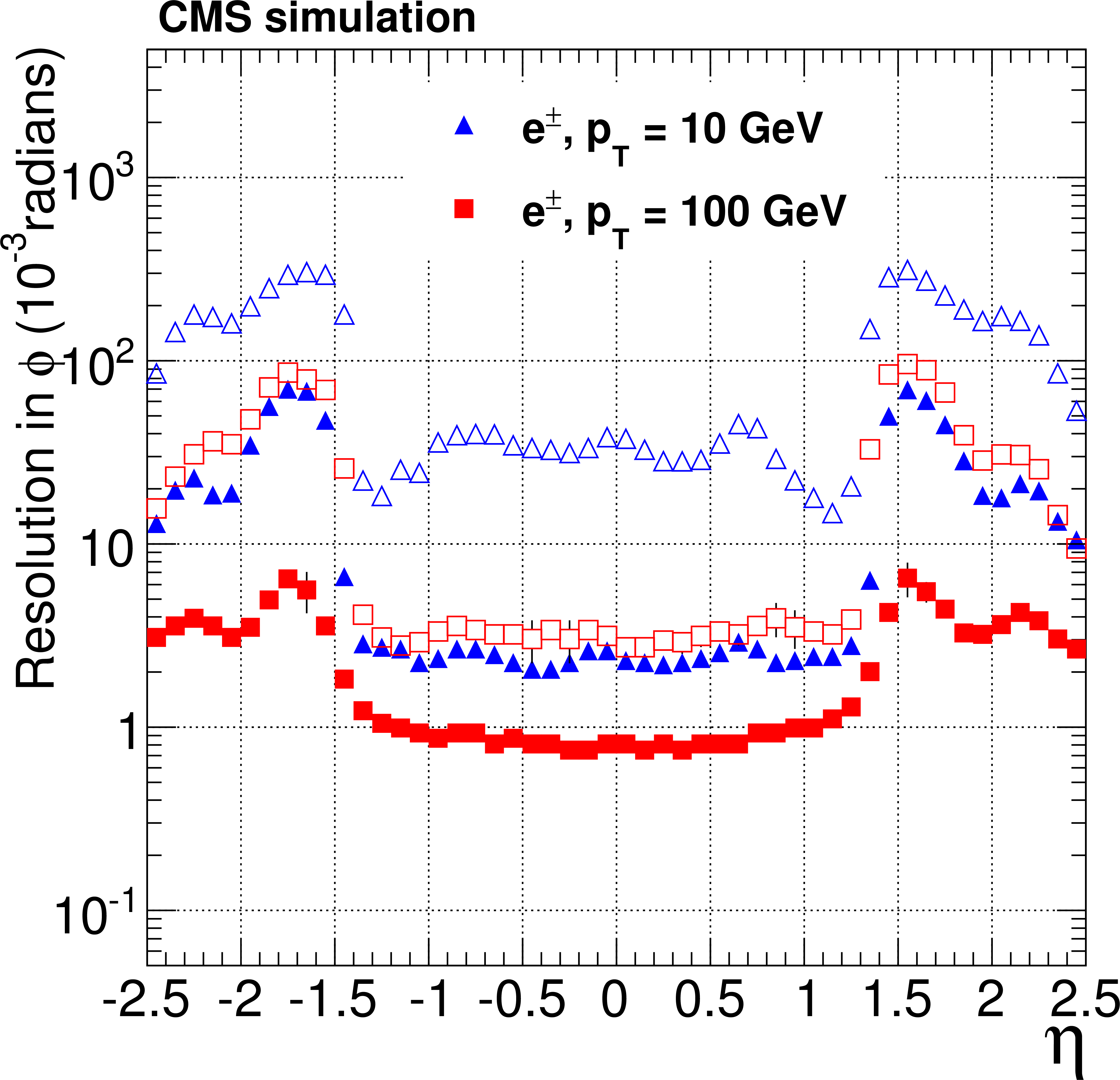
png pdf |
Figure 17-c:
Resolution, as a function of pseudorapidity, in the $d_0$, $\phi $ and $ {p_{\mathrm {T}}} $ track parameters for single, isolated electrons with $ {p_{\mathrm {T}}} = 10$ and 100 GeV. For each bin in $\eta $, the solid (open) symbols correspond to the width of the 68% (90%) intervals having its origin on the mode of the distribution in residuals, as described in the text. Only the half of the residuals distribution that does contain the non-Gaussian tail due to bremsstrahlung is considered in the interval calculation. The a, c, e (b, d, f) plots are of electrons reconstructed with the CTF (GSF) algorithm. |
png pdf |
Figure 17-d:
Resolution, as a function of pseudorapidity, in the $d_0$, $\phi $ and $ {p_{\mathrm {T}}} $ track parameters for single, isolated electrons with $ {p_{\mathrm {T}}} = 10$ and 100 GeV. For each bin in $\eta $, the solid (open) symbols correspond to the width of the 68% (90%) intervals having its origin on the mode of the distribution in residuals, as described in the text. Only the half of the residuals distribution that does contain the non-Gaussian tail due to bremsstrahlung is considered in the interval calculation. The a, c, e (b, d, f) plots are of electrons reconstructed with the CTF (GSF) algorithm. |
png pdf |
Figure 17-e:
Resolution, as a function of pseudorapidity, in the $d_0$, $\phi $ and $ {p_{\mathrm {T}}} $ track parameters for single, isolated electrons with $ {p_{\mathrm {T}}} = 10$ and 100 GeV. For each bin in $\eta $, the solid (open) symbols correspond to the width of the 68% (90%) intervals having its origin on the mode of the distribution in residuals, as described in the text. Only the half of the residuals distribution that does contain the non-Gaussian tail due to bremsstrahlung is considered in the interval calculation. The a, c, e (b, d, f) plots are of electrons reconstructed with the CTF (GSF) algorithm. |
png pdf |
Figure 17-f:
Resolution, as a function of pseudorapidity, in the $d_0$, $\phi $ and $ {p_{\mathrm {T}}} $ track parameters for single, isolated electrons with $ {p_{\mathrm {T}}} = 10$ and 100 GeV. For each bin in $\eta $, the solid (open) symbols correspond to the width of the 68% (90%) intervals having its origin on the mode of the distribution in residuals, as described in the text. Only the half of the residuals distribution that does contain the non-Gaussian tail due to bremsstrahlung is considered in the interval calculation. The a, c, e (b, d, f) plots are of electrons reconstructed with the CTF (GSF) algorithm. |
png pdf |
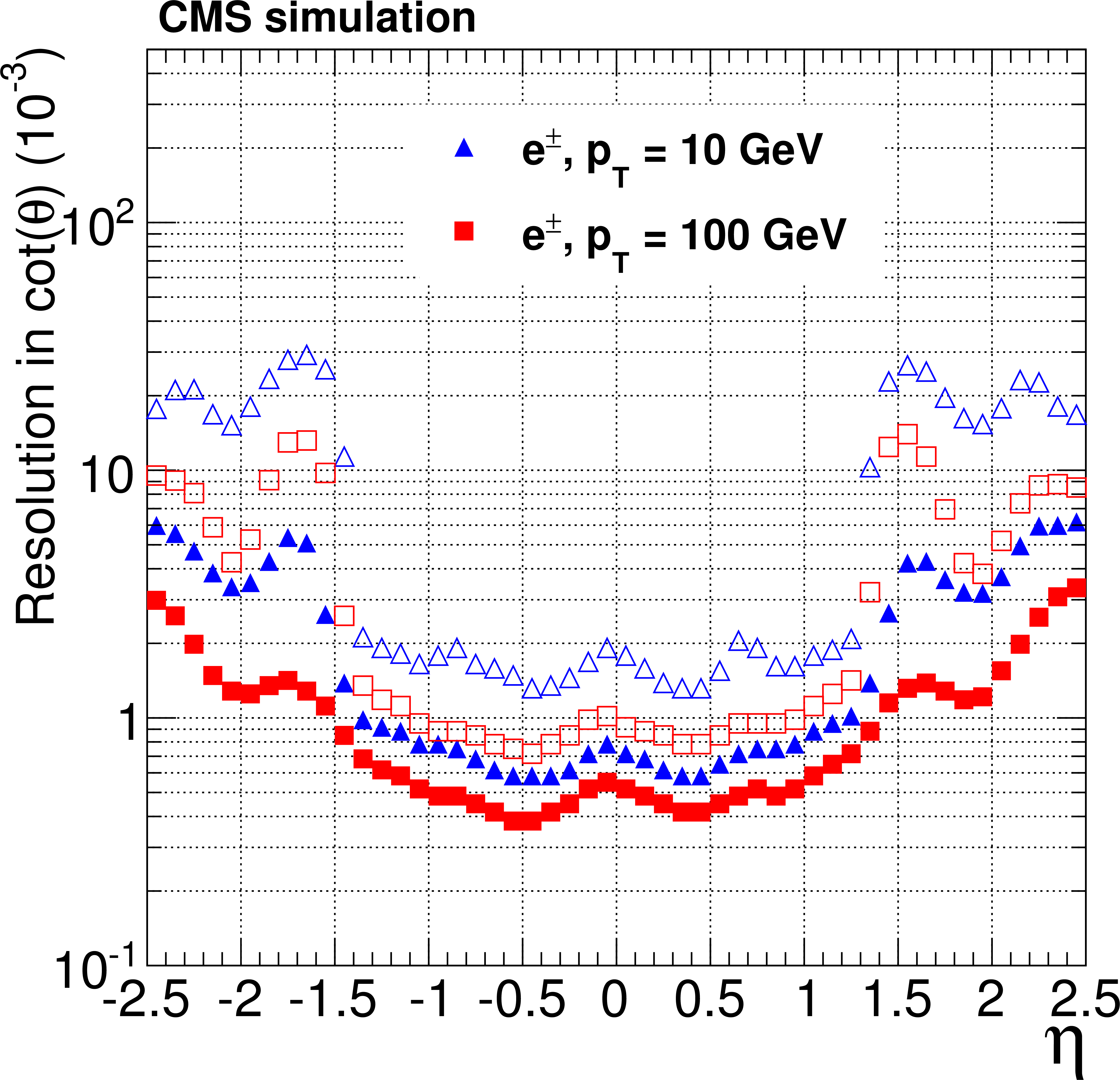
Figure 18-a:
Resolution, as a function of pseudorapidity, in the $\mathrm{ cotan }\theta $ and $z_0$ track parameters for single, isolated electrons with $ {p_{\mathrm {T}}} = 10$ and 100 GeV. For each bin in $\eta $, the solid (open) symbols correspond to the half-width of the 68% (90%) intervals centered on the mode of the distribution in residuals, as described in the text. The a, c (b, d) plots are of electrons reconstructed with the CTF (GSF) algorithm. |
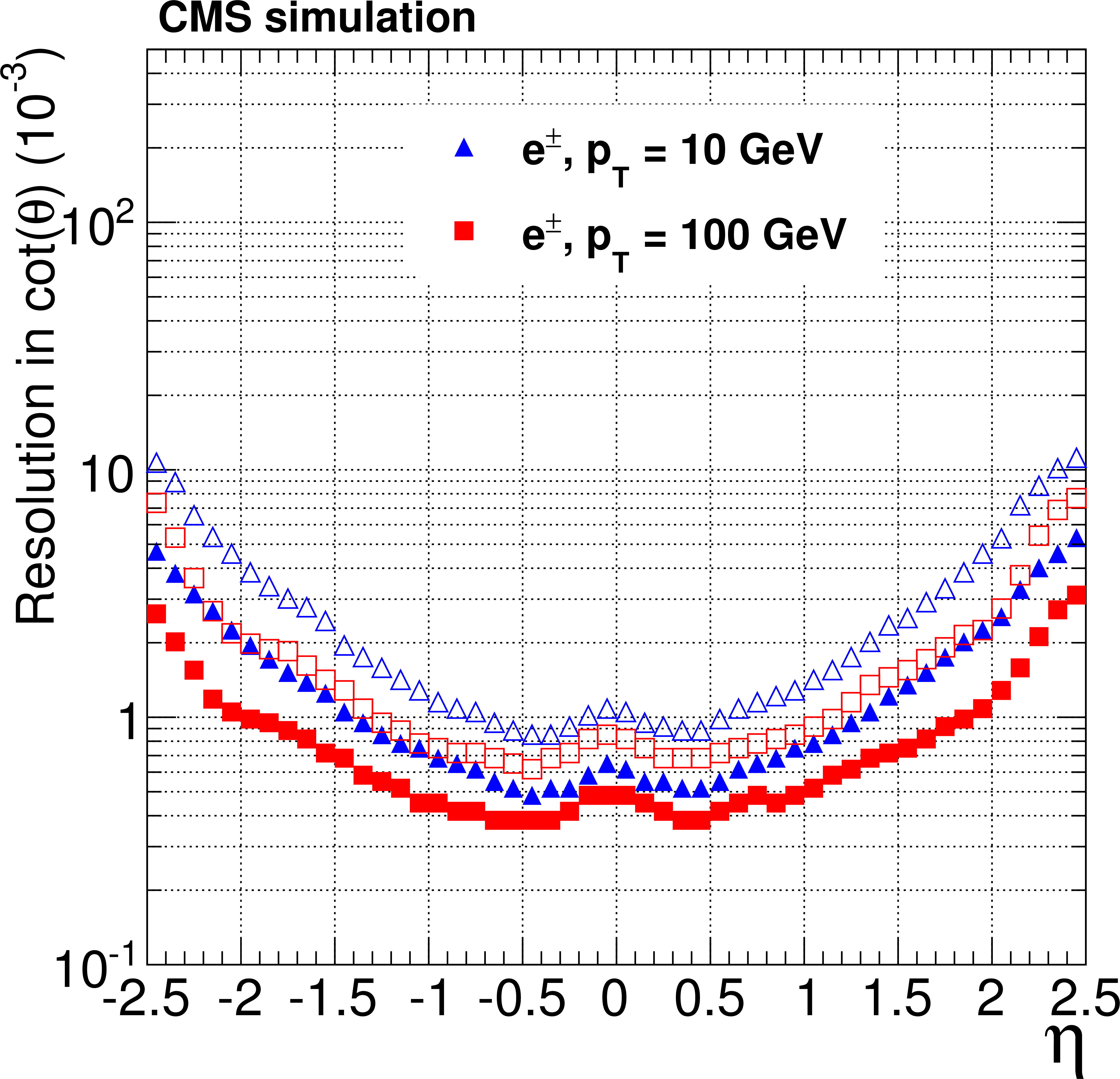
png pdf |
Figure 18-b:
Resolution, as a function of pseudorapidity, in the $\mathrm{ cotan }\theta $ and $z_0$ track parameters for single, isolated electrons with $ {p_{\mathrm {T}}} = 10$ and 100 GeV. For each bin in $\eta $, the solid (open) symbols correspond to the half-width of the 68% (90%) intervals centered on the mode of the distribution in residuals, as described in the text. The a, c (b, d) plots are of electrons reconstructed with the CTF (GSF) algorithm. |

png pdf |
Figure 18-c:
Resolution, as a function of pseudorapidity, in the $\mathrm{ cotan }\theta $ and $z_0$ track parameters for single, isolated electrons with $ {p_{\mathrm {T}}} = 10$ and 100 GeV. For each bin in $\eta $, the solid (open) symbols correspond to the half-width of the 68% (90%) intervals centered on the mode of the distribution in residuals, as described in the text. The a, c (b, d) plots are of electrons reconstructed with the CTF (GSF) algorithm. |
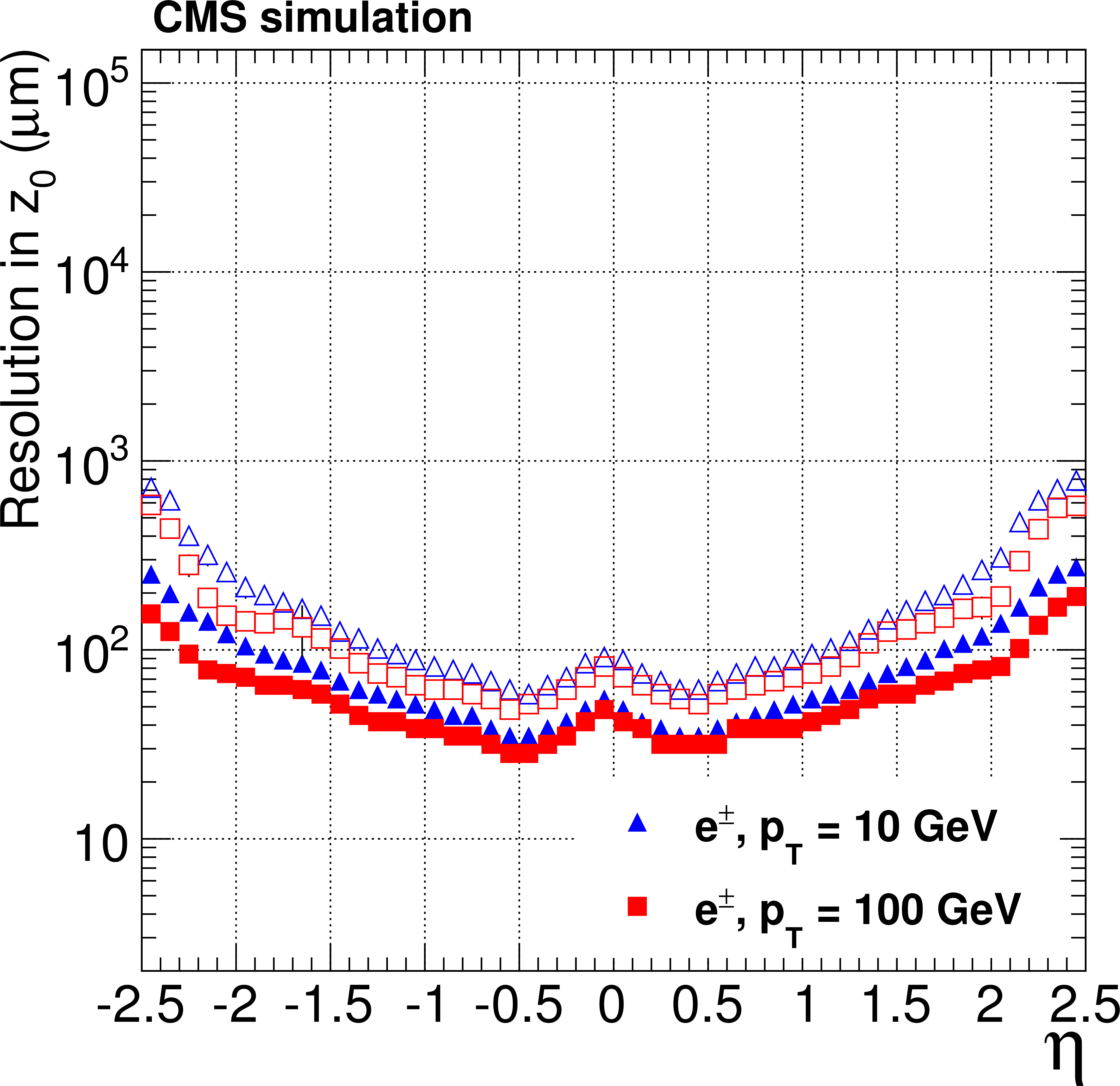
png pdf |
Figure 18-d:
Resolution, as a function of pseudorapidity, in the $\mathrm{ cotan }\theta $ and $z_0$ track parameters for single, isolated electrons with $ {p_{\mathrm {T}}} = 10$ and 100 GeV. For each bin in $\eta $, the solid (open) symbols correspond to the half-width of the 68% (90%) intervals centered on the mode of the distribution in residuals, as described in the text. The a, c (b, d) plots are of electrons reconstructed with the CTF (GSF) algorithm. |
png pdf |
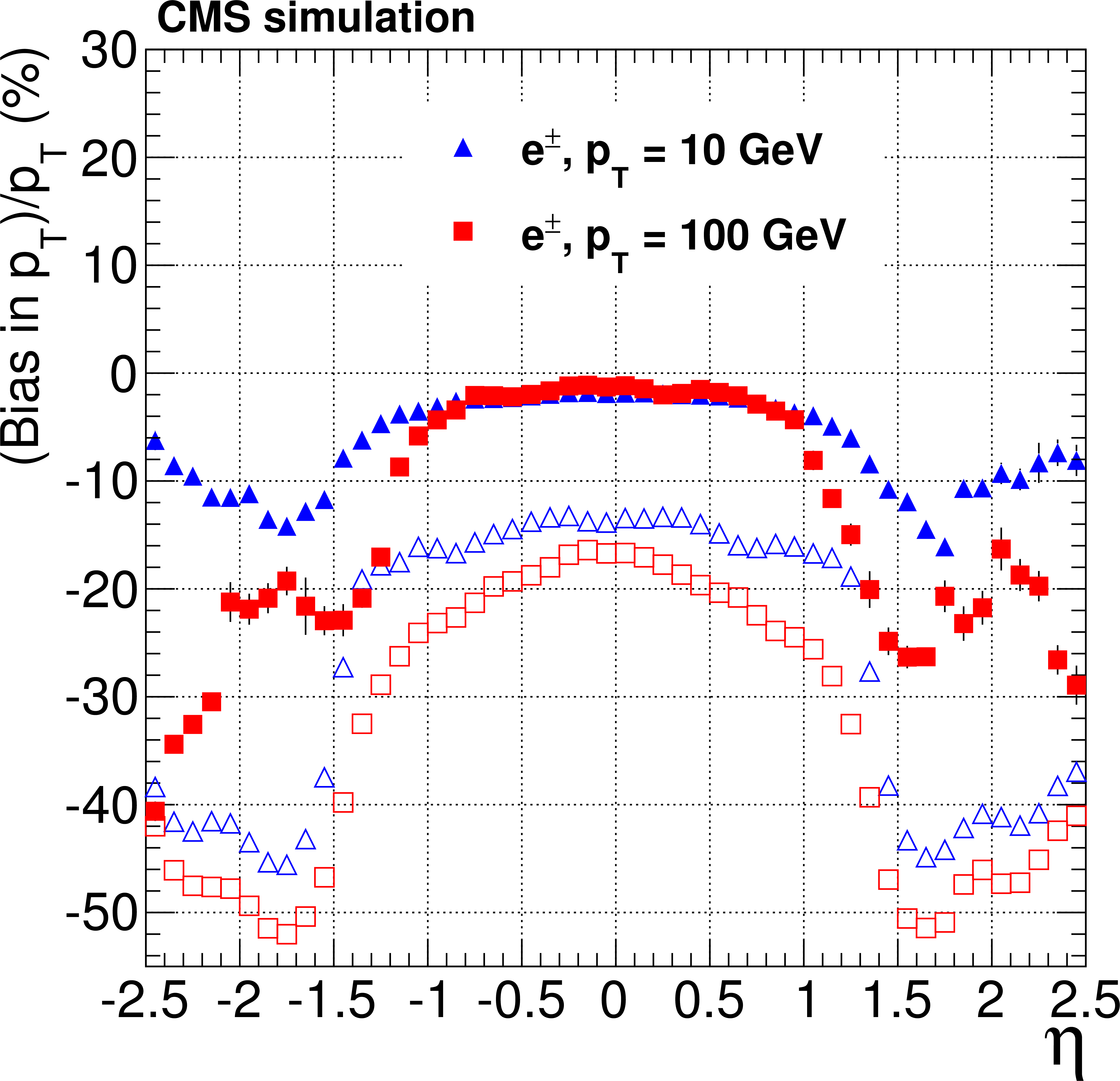
Figure 19-a:
Bias, as a function of pseudorapidity, on the $ {p_{\mathrm {T}}} $ track parameter for single, isolated electrons with $ {p_{\mathrm {T}}} = 10$ and 100 GeV. For each bin in $\eta $, the solid (open) symbols correspond to the mode (mean) of the distribution in residuals. The a (b) plots are of electrons reconstructed with the CTF (GSF) algorithm. |
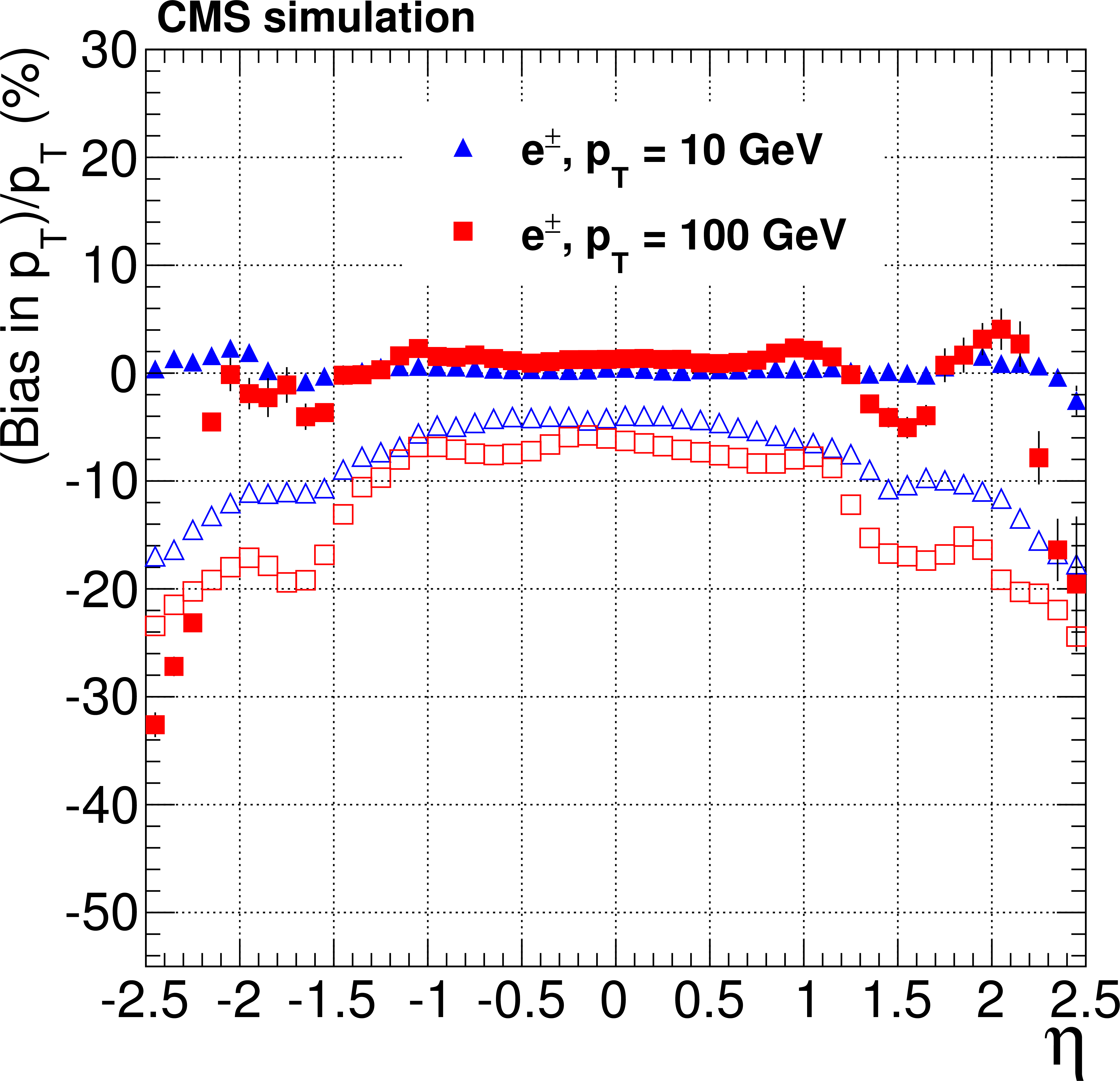
png pdf |
Figure 19-b:
Bias, as a function of pseudorapidity, on the $ {p_{\mathrm {T}}} $ track parameter for single, isolated electrons with $ {p_{\mathrm {T}}} = 10$ and 100 GeV. For each bin in $\eta $, the solid (open) symbols correspond to the mode (mean) of the distribution in residuals. The a (b) plots are of electrons reconstructed with the CTF (GSF) algorithm. |
png pdf |
Figure 20-a:
Resolution, as a function of $ {p_{\mathrm {T}}} $, in the five track parameters for charged particles in simulated $ \mathrm{ t \bar{t} } $ events with pileup. The number of pileup interactions superimposed to each simulated event is generated randomly from a Poisson distribution with a mean value of 8. From a to e: transverse and longitudinal impact parameters, $\phi $, $\mathrm{ cotan }\theta $, and $ {p_{\mathrm {T}}} $ . For each bin in $ {p_{\mathrm {T}}} $, the solid (open) symbols correspond to the half-width of the 68% (90%) intervals centered on the mode of the distribution in residuals, as described in the text. |
png pdf |
Figure 20-b:
Resolution, as a function of $ {p_{\mathrm {T}}} $, in the five track parameters for charged particles in simulated $ \mathrm{ t \bar{t} } $ events with pileup. The number of pileup interactions superimposed to each simulated event is generated randomly from a Poisson distribution with a mean value of 8. From a to e: transverse and longitudinal impact parameters, $\phi $, $\mathrm{ cotan }\theta $, and $ {p_{\mathrm {T}}} $ . For each bin in $ {p_{\mathrm {T}}} $, the solid (open) symbols correspond to the half-width of the 68% (90%) intervals centered on the mode of the distribution in residuals, as described in the text. |
png pdf |
Figure 20-c:
Resolution, as a function of $ {p_{\mathrm {T}}} $, in the five track parameters for charged particles in simulated $ \mathrm{ t \bar{t} } $ events with pileup. The number of pileup interactions superimposed to each simulated event is generated randomly from a Poisson distribution with a mean value of 8. From a to e: transverse and longitudinal impact parameters, $\phi $, $\mathrm{ cotan }\theta $, and $ {p_{\mathrm {T}}} $ . For each bin in $ {p_{\mathrm {T}}} $, the solid (open) symbols correspond to the half-width of the 68% (90%) intervals centered on the mode of the distribution in residuals, as described in the text. |

png pdf |
Figure 20-d:
Resolution, as a function of $ {p_{\mathrm {T}}} $, in the five track parameters for charged particles in simulated $ \mathrm{ t \bar{t} } $ events with pileup. The number of pileup interactions superimposed to each simulated event is generated randomly from a Poisson distribution with a mean value of 8. From a to e: transverse and longitudinal impact parameters, $\phi $, $\mathrm{ cotan }\theta $, and $ {p_{\mathrm {T}}} $ . For each bin in $ {p_{\mathrm {T}}} $, the solid (open) symbols correspond to the half-width of the 68% (90%) intervals centered on the mode of the distribution in residuals, as described in the text. |

png pdf |
Figure 20-e:
Resolution, as a function of $ {p_{\mathrm {T}}} $, in the five track parameters for charged particles in simulated $ \mathrm{ t \bar{t} } $ events with pileup. The number of pileup interactions superimposed to each simulated event is generated randomly from a Poisson distribution with a mean value of 8. From a to e: transverse and longitudinal impact parameters, $\phi $, $\mathrm{ cotan }\theta $, and $ {p_{\mathrm {T}}} $ . For each bin in $ {p_{\mathrm {T}}} $, the solid (open) symbols correspond to the half-width of the 68% (90%) intervals centered on the mode of the distribution in residuals, as described in the text. |

png pdf |
Figure 21:
The number of additional tracks per event reconstructed after each individual iteration, for $ \mathrm{ t \bar{t} } $ events generated without pileup and with an average of 8 pileup events. The distributions include only tracks associated with a simulated charged particle. |
png pdf |
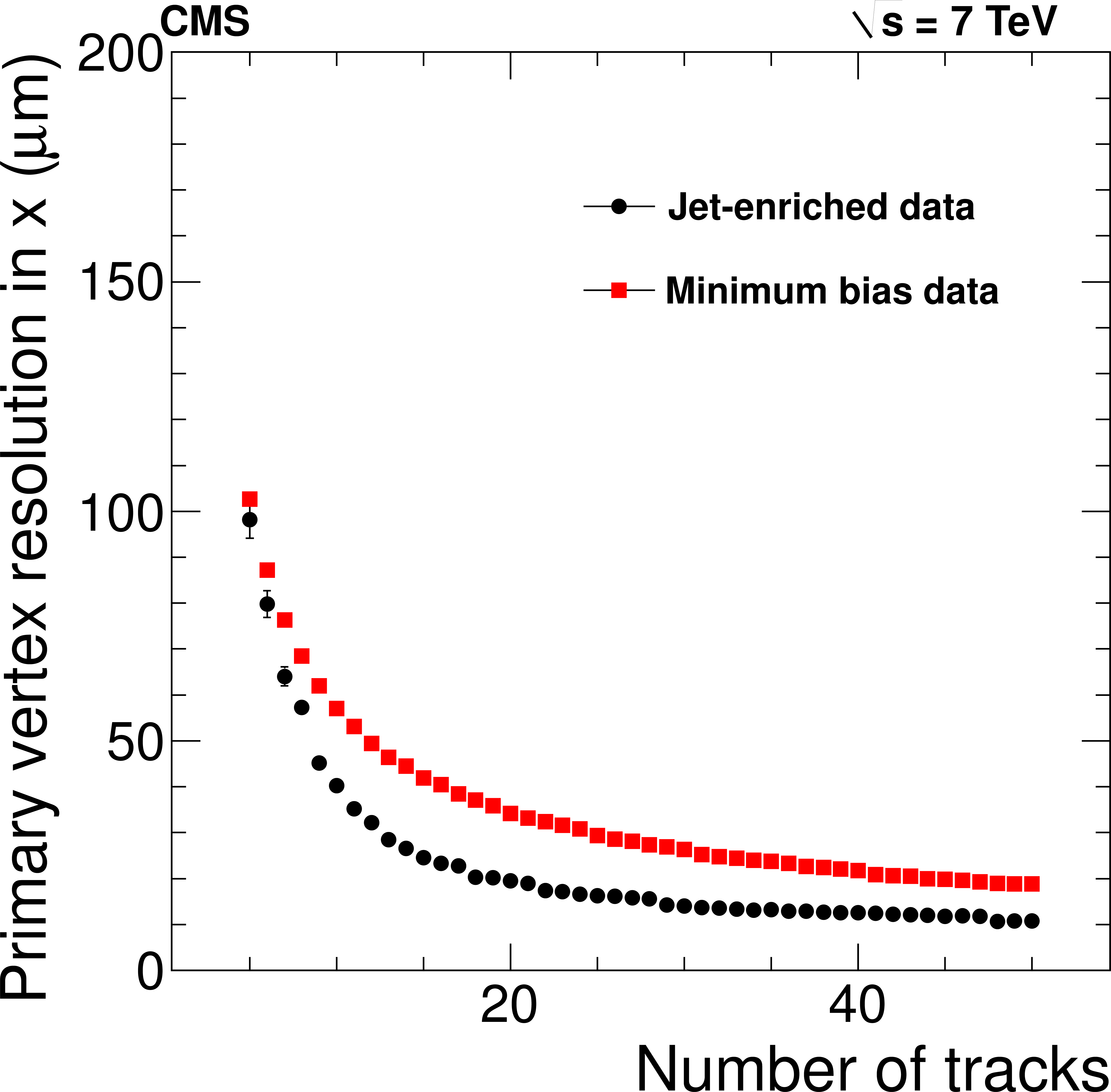
Figure 22-a:
Primary-vertex resolution in $x$ (a) and in $z$ (b) as a function of the number of tracks at the fitted vertex, for two kinds of events with different average track $ {p_{\mathrm {T}}} $ values (see text). |
png pdf |
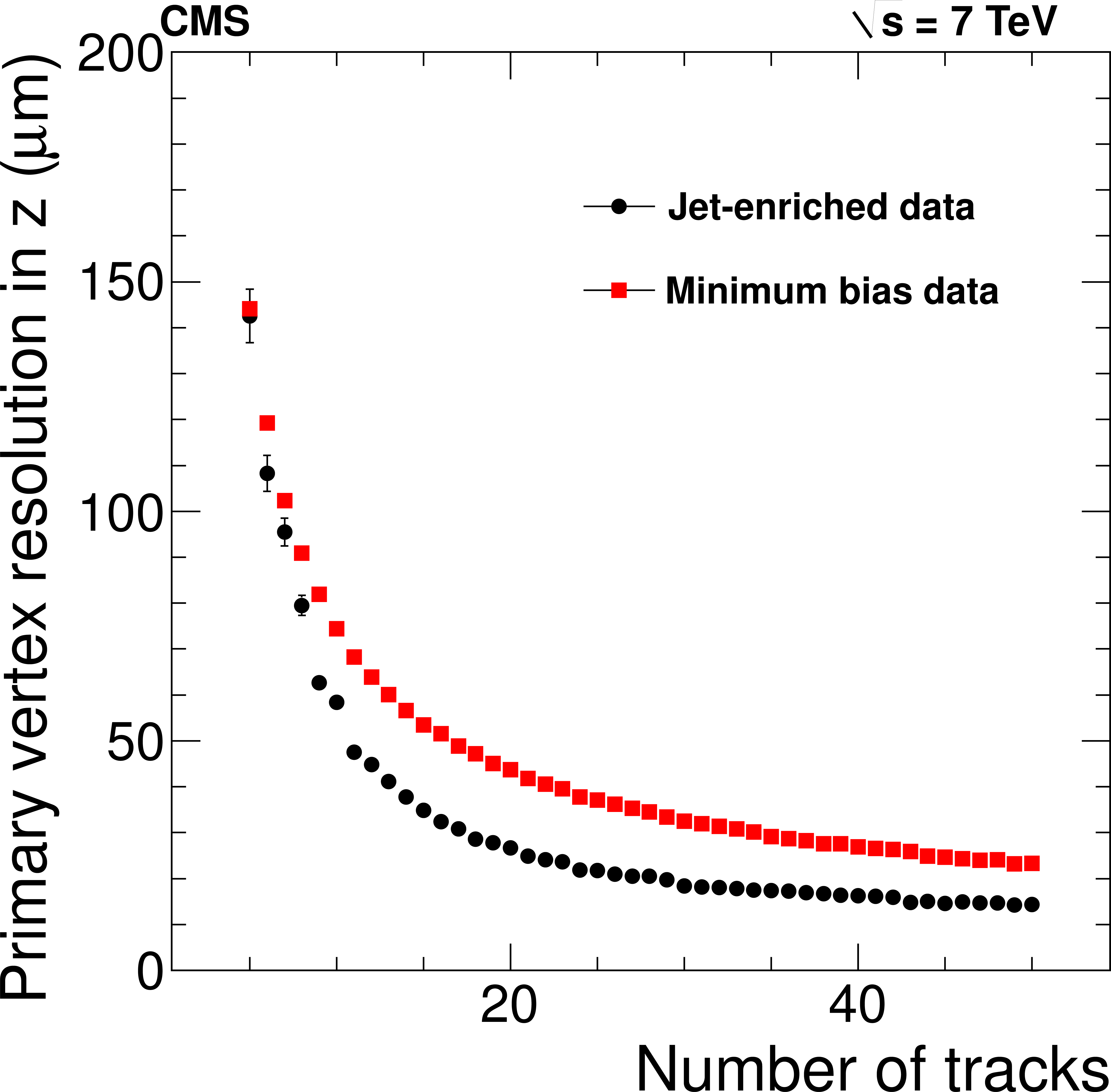
Figure 22-b:
Primary-vertex resolution in $x$ (a) and in $z$ (b) as a function of the number of tracks at the fitted vertex, for two kinds of events with different average track $ {p_{\mathrm {T}}} $ values (see text). |
png pdf |
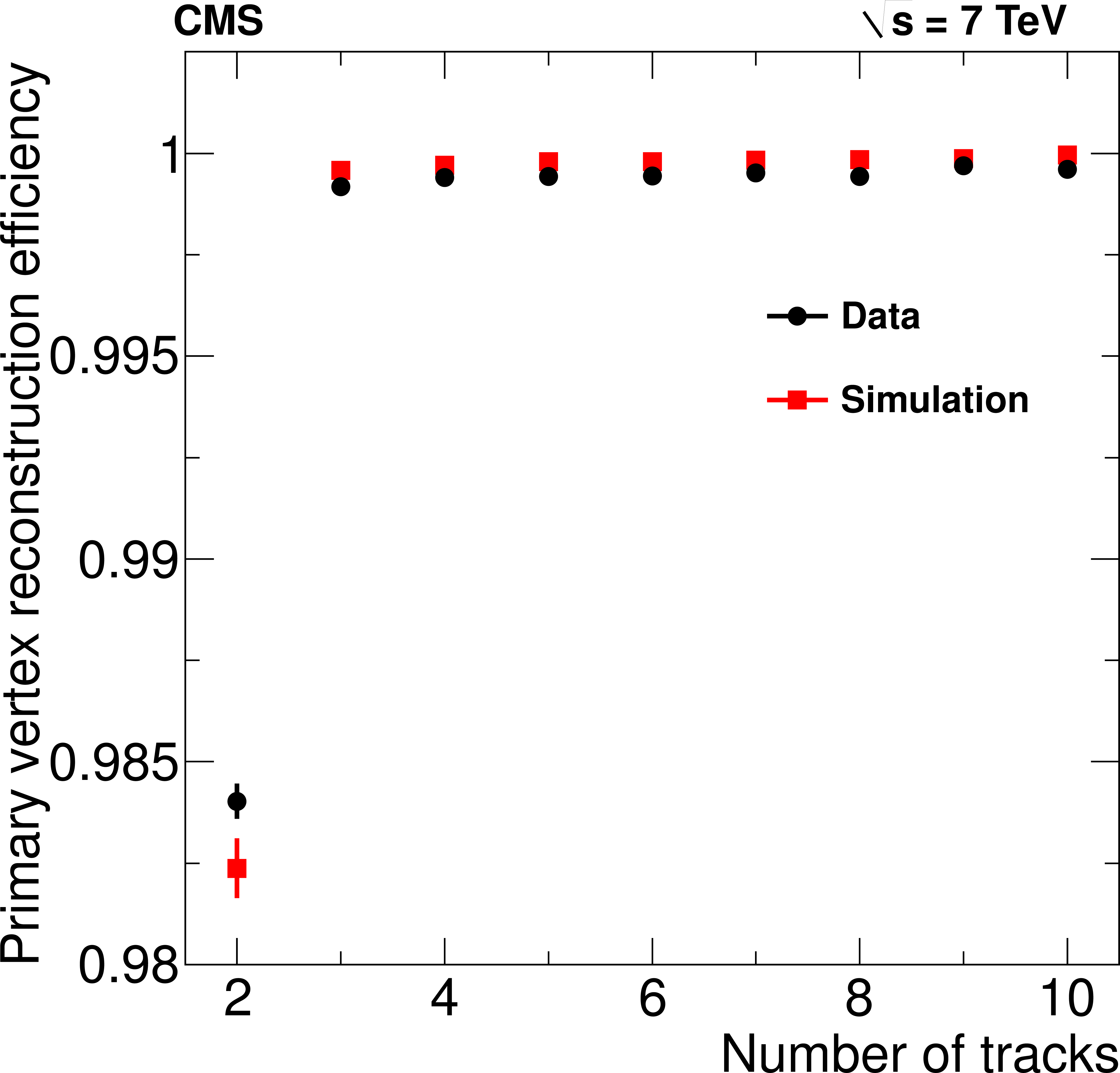
Figure 23:
Primary-vertex reconstruction efficiency as a function of the number of tracks in a cluster, measured in minimum-bias data and in MC simulation. |
png pdf |
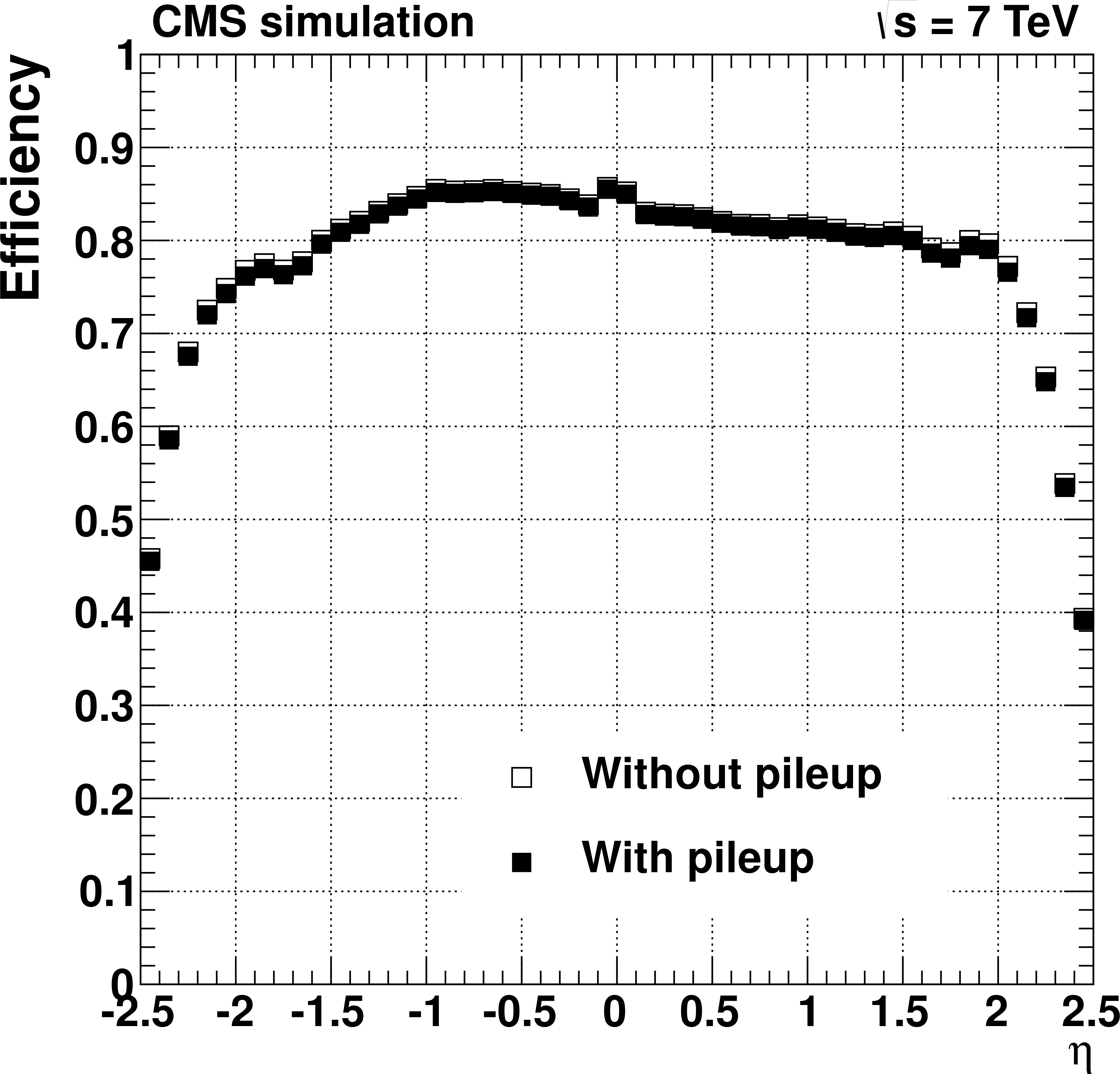
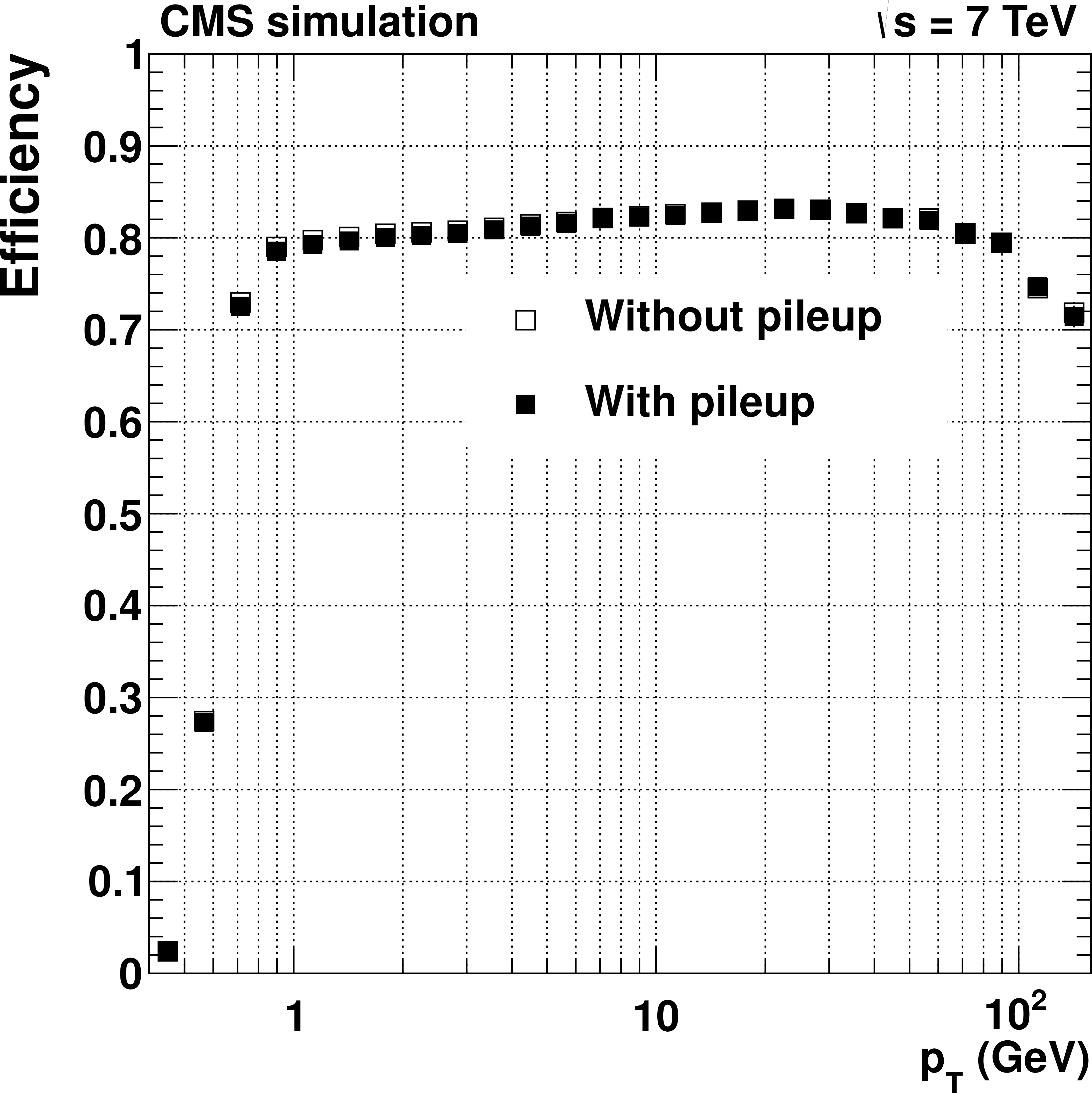
Figure 24-a:
Pixel tracking efficiency (a, b) and fake rate (c, d) for $ \mathrm{ t \bar{t} } $ events simulated with and without superimposed pileup collisions. The number of pileup interactions superimposed on each simulated event is randomly generated from a Poisson distribution with mean equal to 8. The two plots of efficiency and fake rate as a function of pseudorapidity are produced applying a $ {p_{\mathrm {T}}} > $ 0.9 GeV selection. |
png pdf |
Figure 24-b:
Pixel tracking efficiency (a, b) and fake rate (c, d) for $ \mathrm{ t \bar{t} } $ events simulated with and without superimposed pileup collisions. The number of pileup interactions superimposed on each simulated event is randomly generated from a Poisson distribution with mean equal to 8. The two plots of efficiency and fake rate as a function of pseudorapidity are produced applying a $ {p_{\mathrm {T}}} > $ 0.9 GeV selection. |
png pdf |
Figure 24-c:
Pixel tracking efficiency (a, b) and fake rate (c, d) for $ \mathrm{ t \bar{t} } $ events simulated with and without superimposed pileup collisions. The number of pileup interactions superimposed on each simulated event is randomly generated from a Poisson distribution with mean equal to 8. The two plots of efficiency and fake rate as a function of pseudorapidity are produced applying a $ {p_{\mathrm {T}}} > $ 0.9 GeV selection. |
png pdf |
Figure 24-d:
Pixel tracking efficiency (a, b) and fake rate (c, d) for $ \mathrm{ t \bar{t} } $ events simulated with and without superimposed pileup collisions. The number of pileup interactions superimposed on each simulated event is randomly generated from a Poisson distribution with mean equal to 8. The two plots of efficiency and fake rate as a function of pseudorapidity are produced applying a $ {p_{\mathrm {T}}} > $ 0.9 GeV selection. |
png pdf |
Figure 25-a:
Resolution, as a function of $ {p_{\mathrm {T}}} $, in the five track parameters for pixel tracks in simulated $ \mathrm{ t \bar{t} } $ events with pileup in the barrel, transition and endcap regions, defined by the pseudorapidity intervals 0-0.9, 0.9-1.4 and 1.4-2.5, respectively. From a to e to right: transverse and longitudinal impact parameters, $\varphi $, $\mathrm{ cotan }\vartheta $ and transverse momentum. For each bin in $ {p_{\mathrm {T}}} $, the solid (open) symbol corresponds to the half-width of the 68% (90%) interval centered on the most probable value of the residuals distributions. |

png pdf |
Figure 25-b:
Resolution, as a function of $ {p_{\mathrm {T}}} $, in the five track parameters for pixel tracks in simulated $ \mathrm{ t \bar{t} } $ events with pileup in the barrel, transition and endcap regions, defined by the pseudorapidity intervals 0-0.9, 0.9-1.4 and 1.4-2.5, respectively. From a to e to right: transverse and longitudinal impact parameters, $\varphi $, $\mathrm{ cotan }\vartheta $ and transverse momentum. For each bin in $ {p_{\mathrm {T}}} $, the solid (open) symbol corresponds to the half-width of the 68% (90%) interval centered on the most probable value of the residuals distributions. |

png pdf |
Figure 25-c:
Resolution, as a function of $ {p_{\mathrm {T}}} $, in the five track parameters for pixel tracks in simulated $ \mathrm{ t \bar{t} } $ events with pileup in the barrel, transition and endcap regions, defined by the pseudorapidity intervals 0-0.9, 0.9-1.4 and 1.4-2.5, respectively. From a to e to right: transverse and longitudinal impact parameters, $\varphi $, $\mathrm{ cotan }\vartheta $ and transverse momentum. For each bin in $ {p_{\mathrm {T}}} $, the solid (open) symbol corresponds to the half-width of the 68% (90%) interval centered on the most probable value of the residuals distributions. |

png pdf |
Figure 25-d:
Resolution, as a function of $ {p_{\mathrm {T}}} $, in the five track parameters for pixel tracks in simulated $ \mathrm{ t \bar{t} } $ events with pileup in the barrel, transition and endcap regions, defined by the pseudorapidity intervals 0-0.9, 0.9-1.4 and 1.4-2.5, respectively. From a to e to right: transverse and longitudinal impact parameters, $\varphi $, $\mathrm{ cotan }\vartheta $ and transverse momentum. For each bin in $ {p_{\mathrm {T}}} $, the solid (open) symbol corresponds to the half-width of the 68% (90%) interval centered on the most probable value of the residuals distributions. |
png pdf |
Figure 25-e:
Resolution, as a function of $ {p_{\mathrm {T}}} $, in the five track parameters for pixel tracks in simulated $ \mathrm{ t \bar{t} } $ events with pileup in the barrel, transition and endcap regions, defined by the pseudorapidity intervals 0-0.9, 0.9-1.4 and 1.4-2.5, respectively. From a to e to right: transverse and longitudinal impact parameters, $\varphi $, $\mathrm{ cotan }\vartheta $ and transverse momentum. For each bin in $ {p_{\mathrm {T}}} $, the solid (open) symbol corresponds to the half-width of the 68% (90%) interval centered on the most probable value of the residuals distributions. |
png pdf |
Figure 26-a:
Pixel vertex position resolutions in $x$ (a) and $z$ (b) as a function of the number of tracks used in the fitted vertex, for minimum-bias and jet-enriched data. |

png pdf |
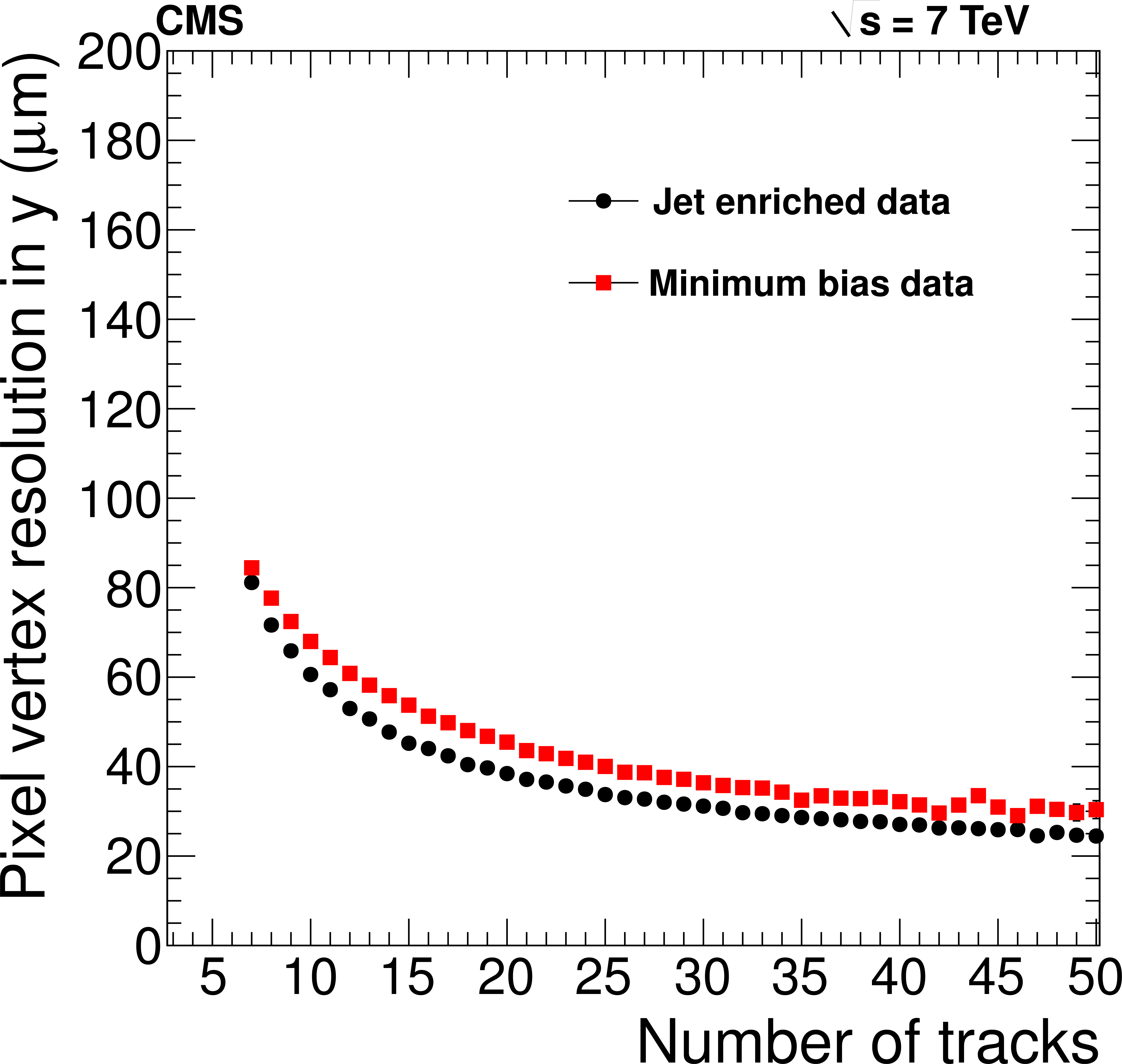
Figure 26-b:
Pixel vertex position resolutions in $x$ (a) and $z$ (b) as a function of the number of tracks used in the fitted vertex, for minimum-bias and jet-enriched data. |
|
|
Compact Muon Solenoid LHC, CERN |
|

|

|

|

|

|