

Compact Muon Solenoid
LHC, CERN
| CMS-TRK-11-002 ; CERN-PH-EP-2014-028 | ||
| Alignment of the CMS tracker with LHC and cosmic ray data | ||
| CMS Collaboration | ||
| 10 March 2014 | ||
| J. Instrum. 9 (2014) P06009 | ||
| Abstract: The central component of the CMS detector is the largest silicon tracker ever built. The precise alignment of this complex device is a formidable challenge, and only achievable with a significant extension of the technologies routinely used for tracking detectors in the past. This article describes the full-scale alignment procedure as it is used during LHC operations. Among the specific features of the method are the simultaneous determination of up to 200,000 alignment parameters with tracks, the measurement of individual sensor curvature parameters, the control of systematic misalignment effects, and the implementation of the whole procedure in a multi-processor environment for high execution speed. Overall, the achieved statistical accuracy on the module alignment is found to be significantly better than 10 microns. | ||
| Links: e-print arXiv:1403.2286 [physics.ins-det] (PDF) ; CDS record ; inSPIRE record ; CADI line (restricted) ; | ||
| Figures | |

png pdf |
Figure 1:
Schematic view of one quarter of the silicon tracker in the $r$-$z$ plane. The positions of the pixel modules are indicated within the hatched area. At larger radii within the lightly shaded areas, solid rectangles represent single strip modules, while hollow rectangles indicate pairs of strip modules mounted back-to-back with a relative stereo angle. The figure also illustrates the paths of the laser rays (R), the alignment tubes (A) and the beam splitters (B) of the laser alignment system. |
png pdf |
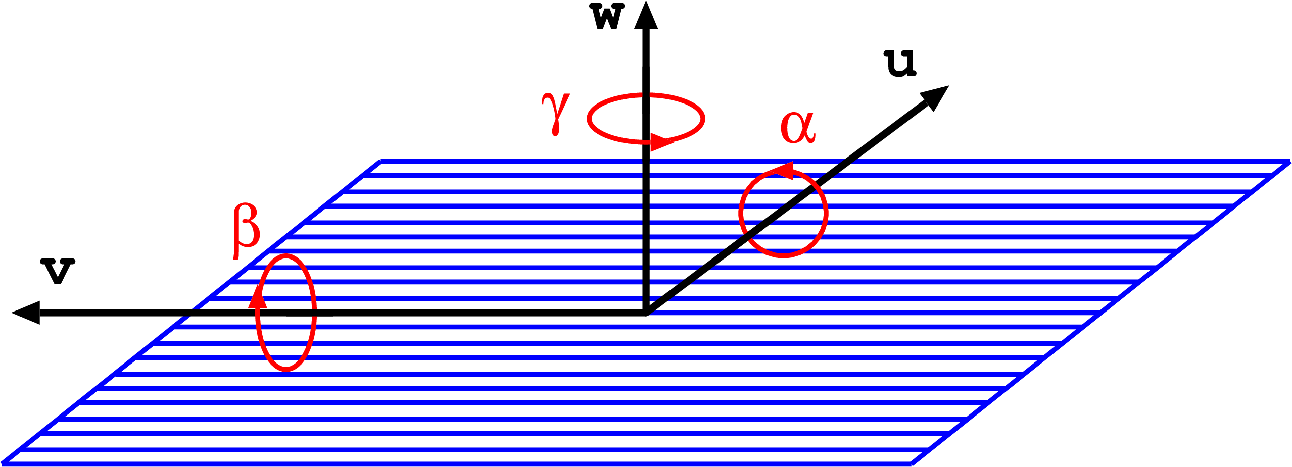
Figure 2-a:
Sketch of a silicon strip module showing the axes of its local coordinate system, $u$, $v$, and $w$, and the respective local rotations $\alpha $, $\beta $, $\gamma $ (a), together with illustrations of the local track angles $\psi $ and $\zeta $ (b). |
png pdf |
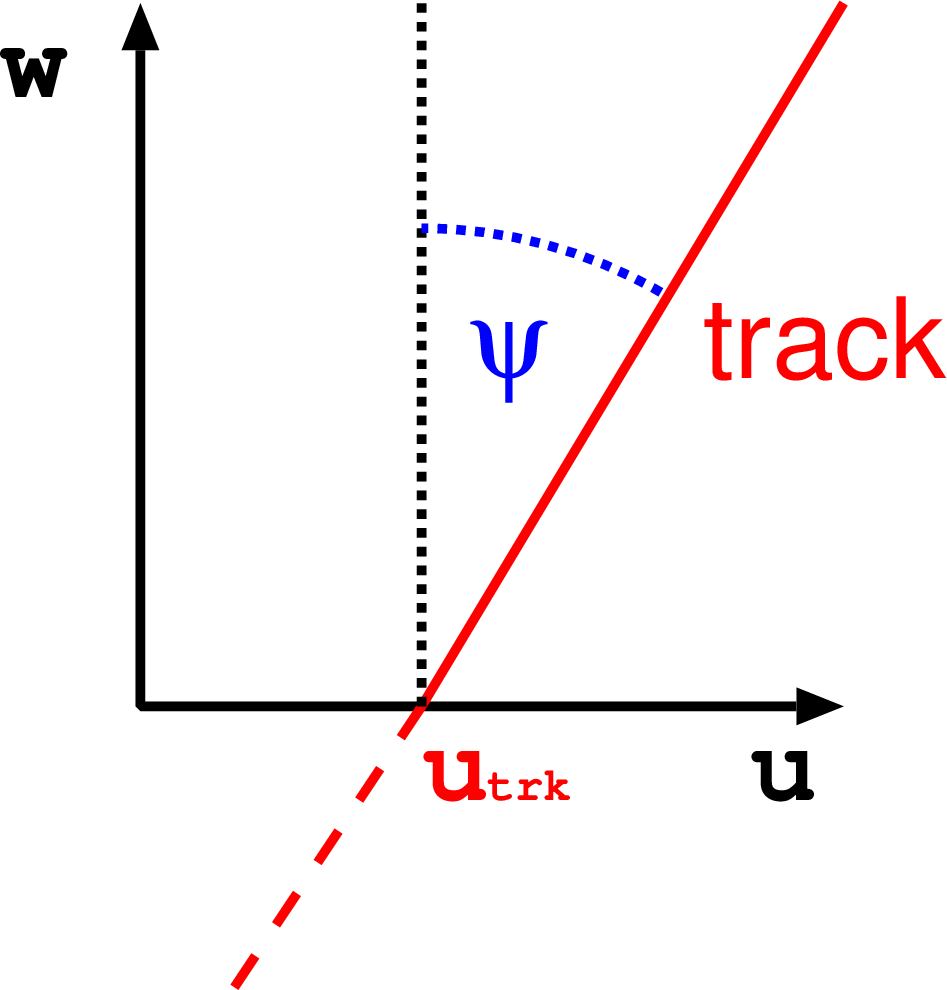
Figure 2-b:
Sketch of a silicon strip module showing the axes of its local coordinate system, $u$, $v$, and $w$, and the respective local rotations $\alpha $, $\beta $, $\gamma $ (a), together with illustrations of the local track angles $\psi $ and $\zeta $ (b). |
png pdf |
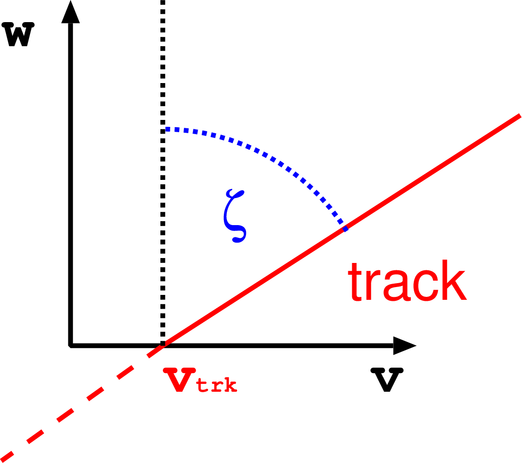
Figure 2-c:
Sketch of a silicon strip module showing the axes of its local coordinate system, $u$, $v$, and $w$, and the respective local rotations $\alpha $, $\beta $, $\gamma $ (a), together with illustrations of the local track angles $\psi $ and $\zeta $ (b). |
png pdf |
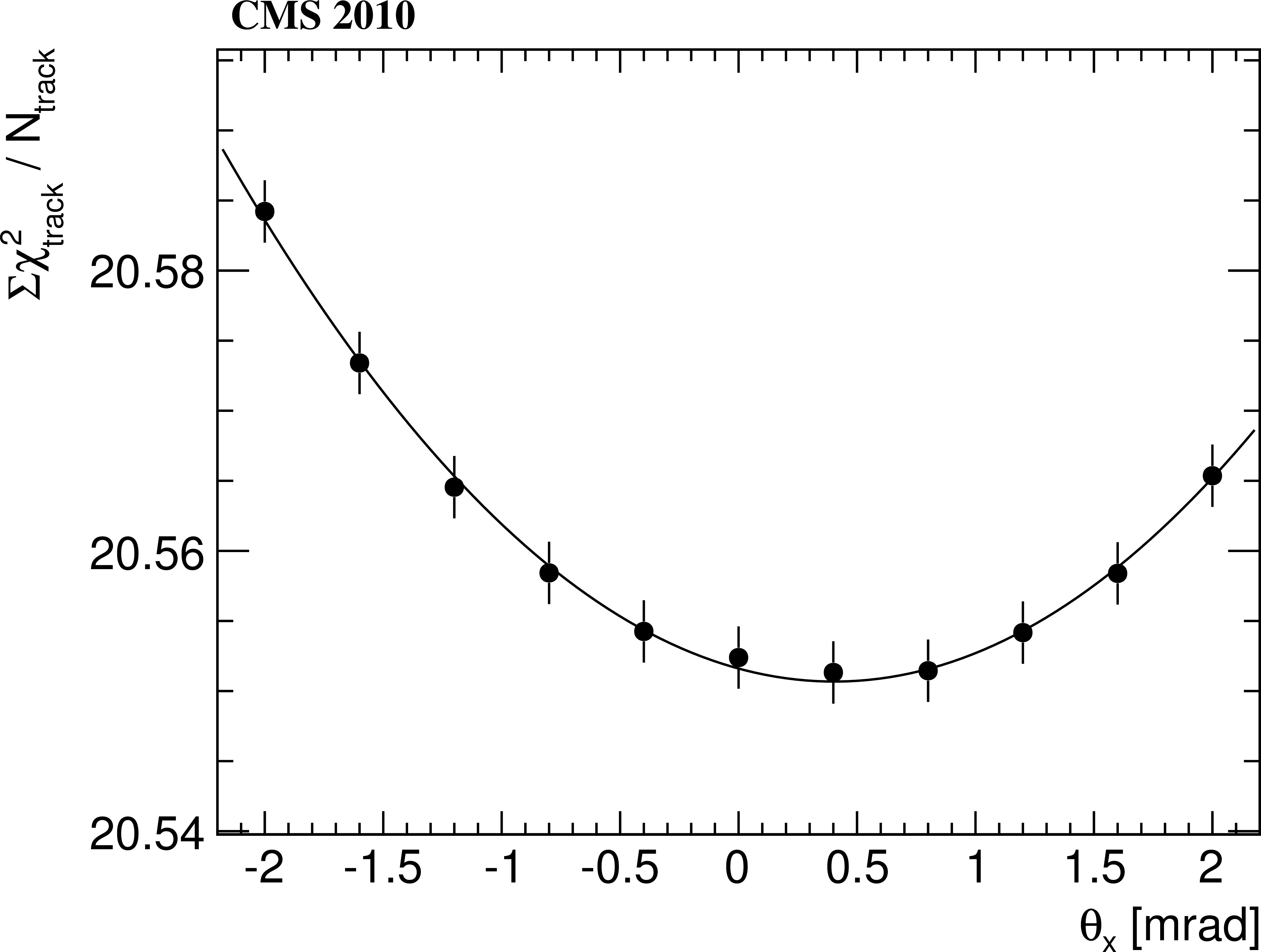
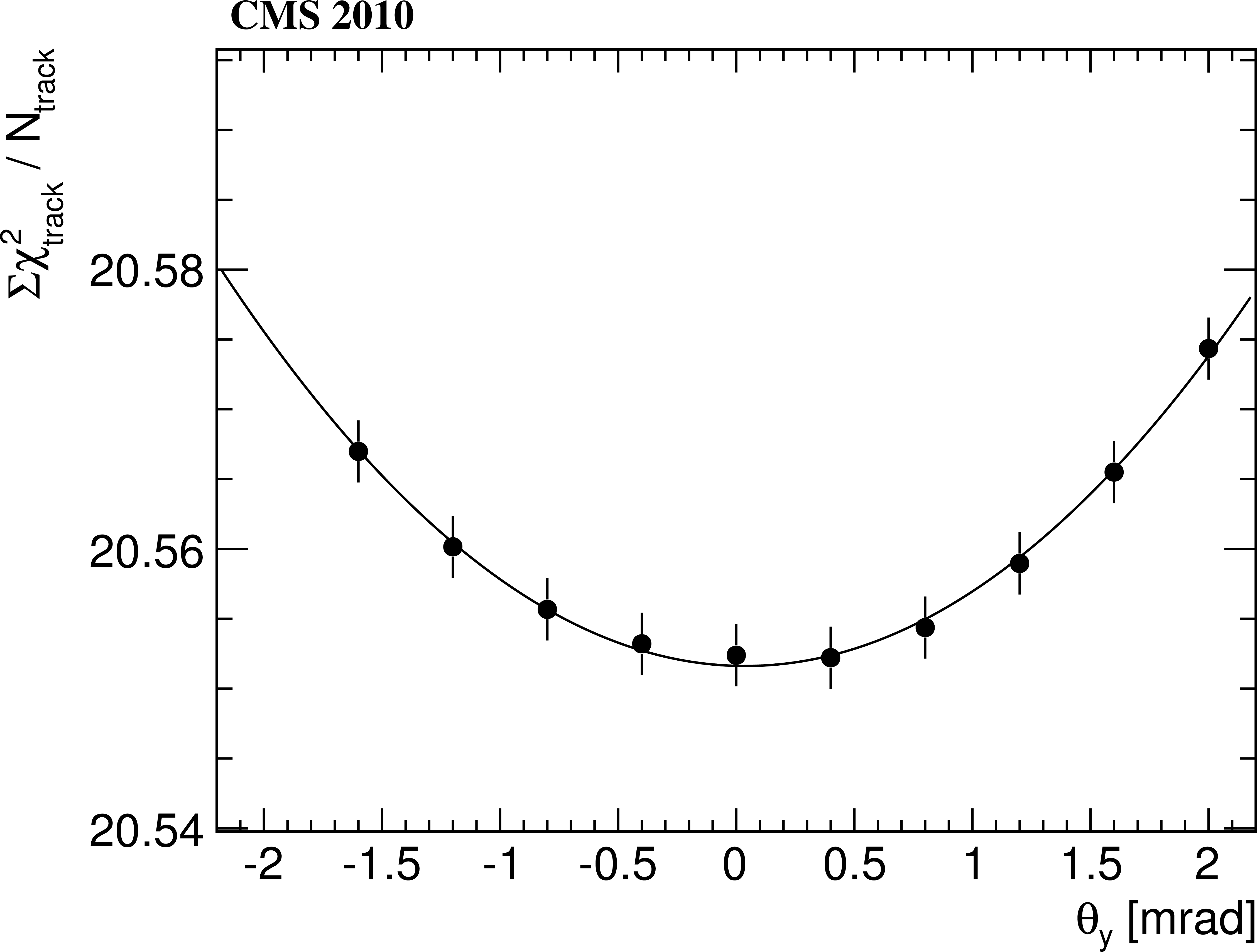
Figure 3-a:
Dependence of the total $\chi ^2$ of the track fits, divided by the number of tracks, on the assumed $\theta _x$ (a) and $\theta _y$ (b) tilt angles for $ {| \eta | } <$ 2.5 and ${p_{\mathrm {T}}} >$ 1 GeV/$c$. The error bars are purely statistical and correlated point-to-point because the same tracks are used for each point. |
png pdf |
Figure 3-b:
Dependence of the total $\chi ^2$ of the track fits, divided by the number of tracks, on the assumed $\theta _x$ (a) and $\theta _y$ (b) tilt angles for $ {| \eta | } <$ 2.5 and ${p_{\mathrm {T}}} >$ 1 GeV/$c$. The error bars are purely statistical and correlated point-to-point because the same tracks are used for each point. |

png pdf |
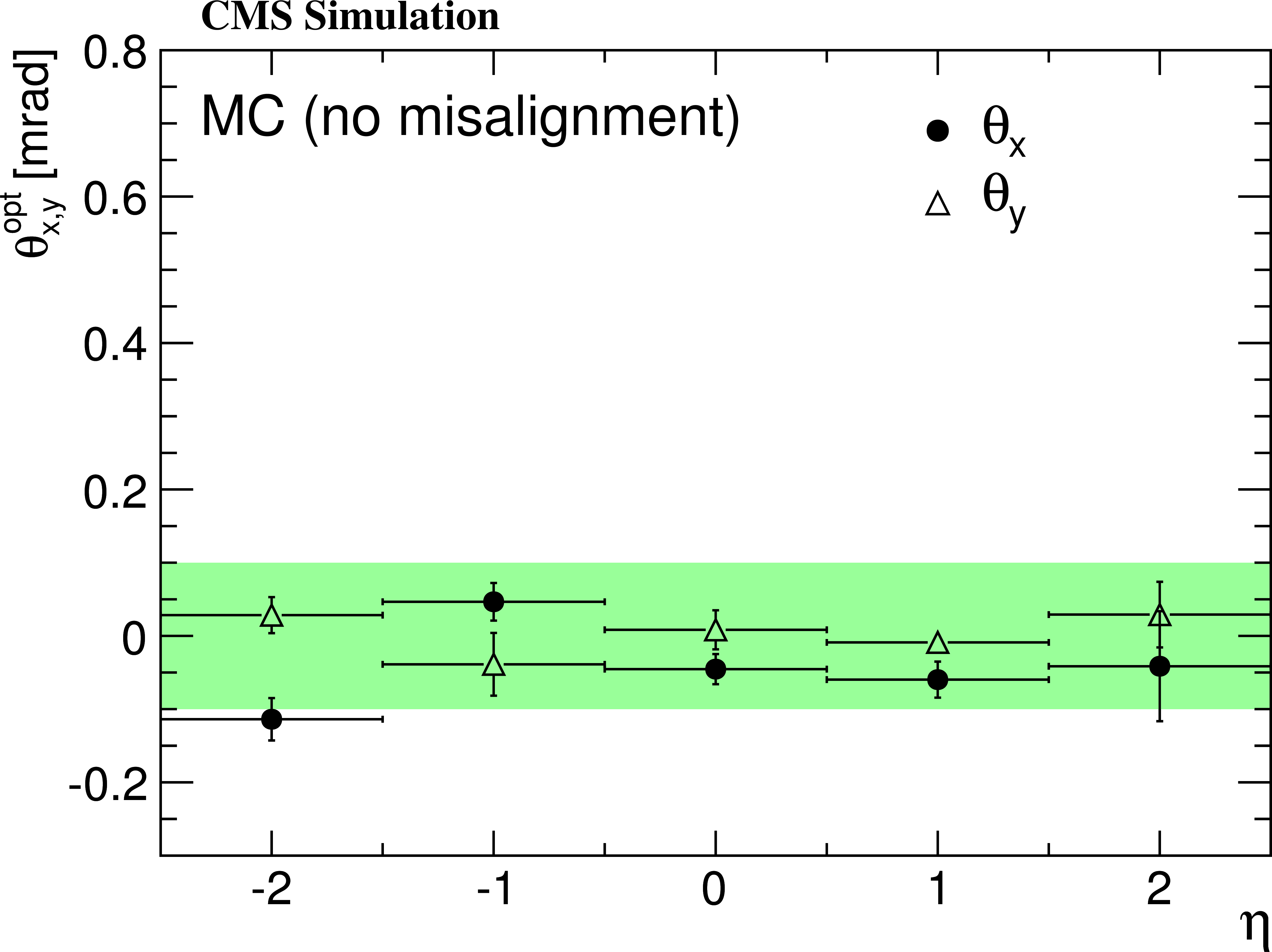
Figure 4-a:
Tracker tilt angles $\theta _x$ (filled circles) and $\theta _y$ (hollow triangles) as a function of track pseudorapidity. The left plot shows the values measured with the data collected in 2010; the right plot has been obtained from simulated events without tracker misalignment. The statistical uncertainty is typically smaller than the symbol size and mostly invisible. The outer error bars indicate the RMS of the variations which are observed when varying several parameters of the tilt angle determination. The shaded bands indicate the margins of $\pm $0.1 discussed in the text. |
png pdf |
Figure 4-b:
Tracker tilt angles $\theta _x$ (filled circles) and $\theta _y$ (hollow triangles) as a function of track pseudorapidity. The left plot shows the values measured with the data collected in 2010; the right plot has been obtained from simulated events without tracker misalignment. The statistical uncertainty is typically smaller than the symbol size and mostly invisible. The outer error bars indicate the RMS of the variations which are observed when varying several parameters of the tilt angle determination. The shaded bands indicate the margins of $\pm $0.1 discussed in the text. |
png pdf |
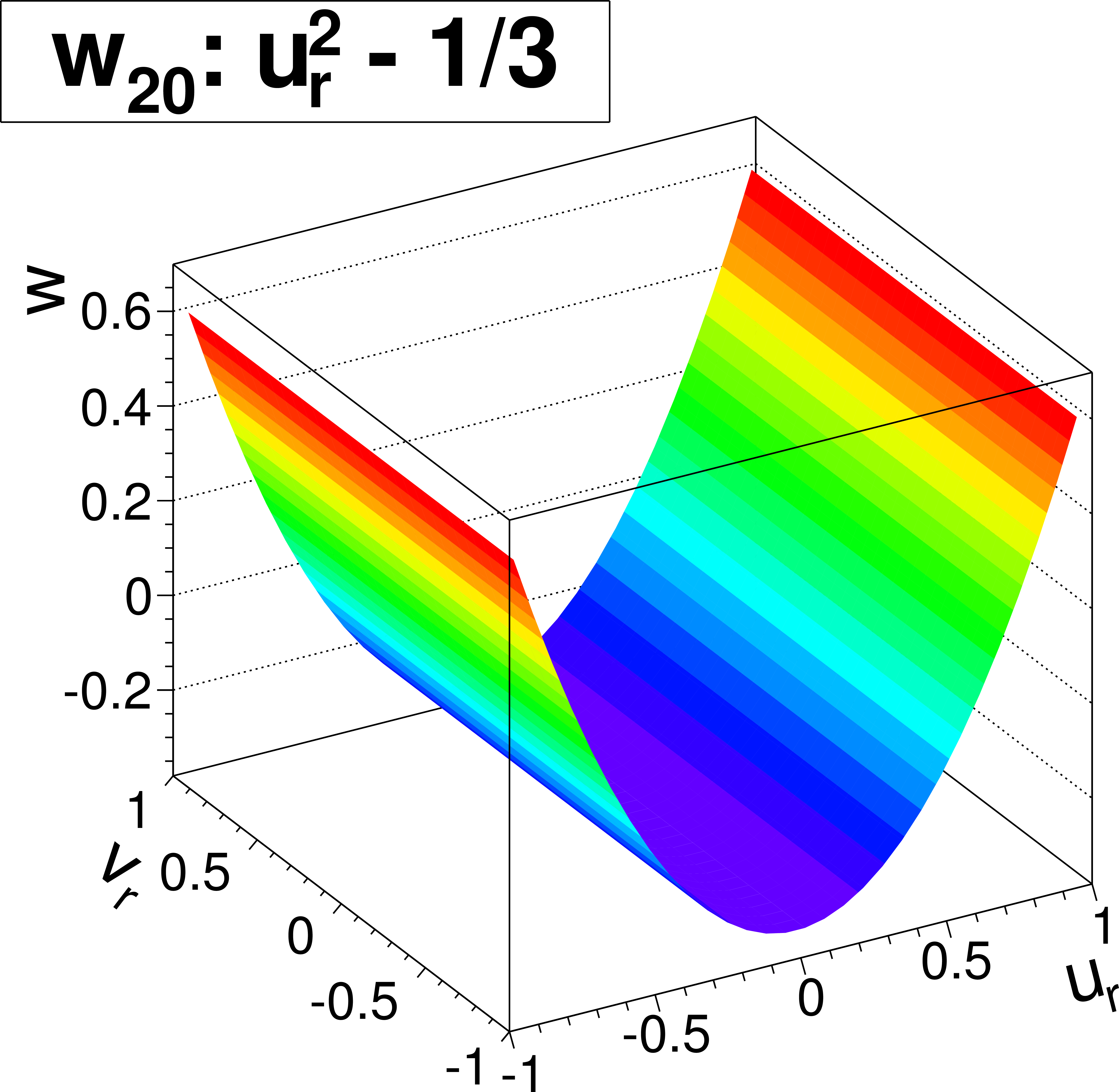
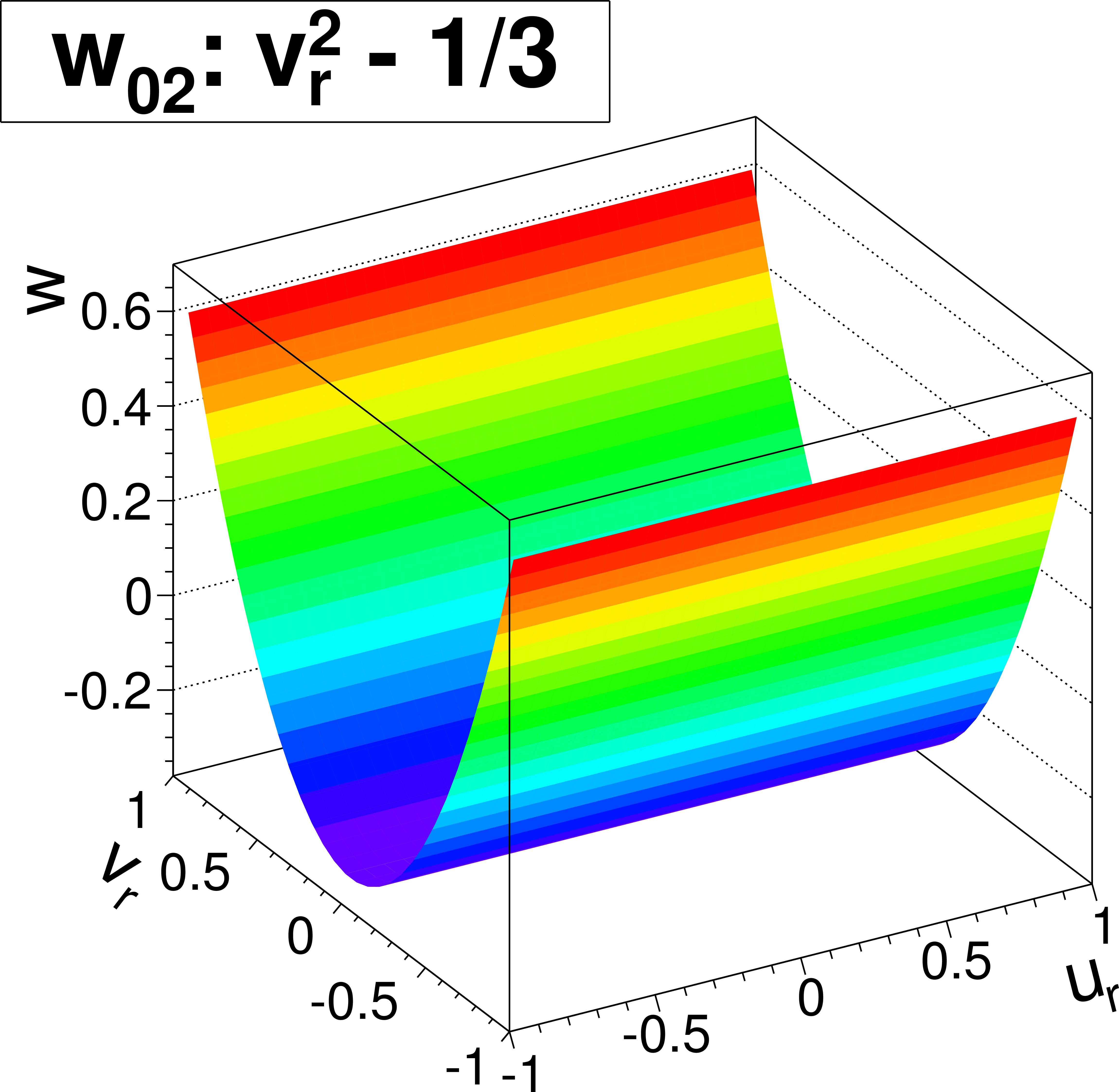
Figure 5-a:
The three two-dimensional second-order polynomials to describe sensor deviations from the flat plane, illustrated for sagittae $w_{20} = w_{11} = w_{02} = 1$. |

png pdf |
Figure 5-b:
The three two-dimensional second-order polynomials to describe sensor deviations from the flat plane, illustrated for sagittae $w_{20} = w_{11} = w_{02} = 1$. |
png pdf |
Figure 5-c:
The three two-dimensional second-order polynomials to describe sensor deviations from the flat plane, illustrated for sagittae $w_{20} = w_{11} = w_{02} = 1$. |
png pdf |
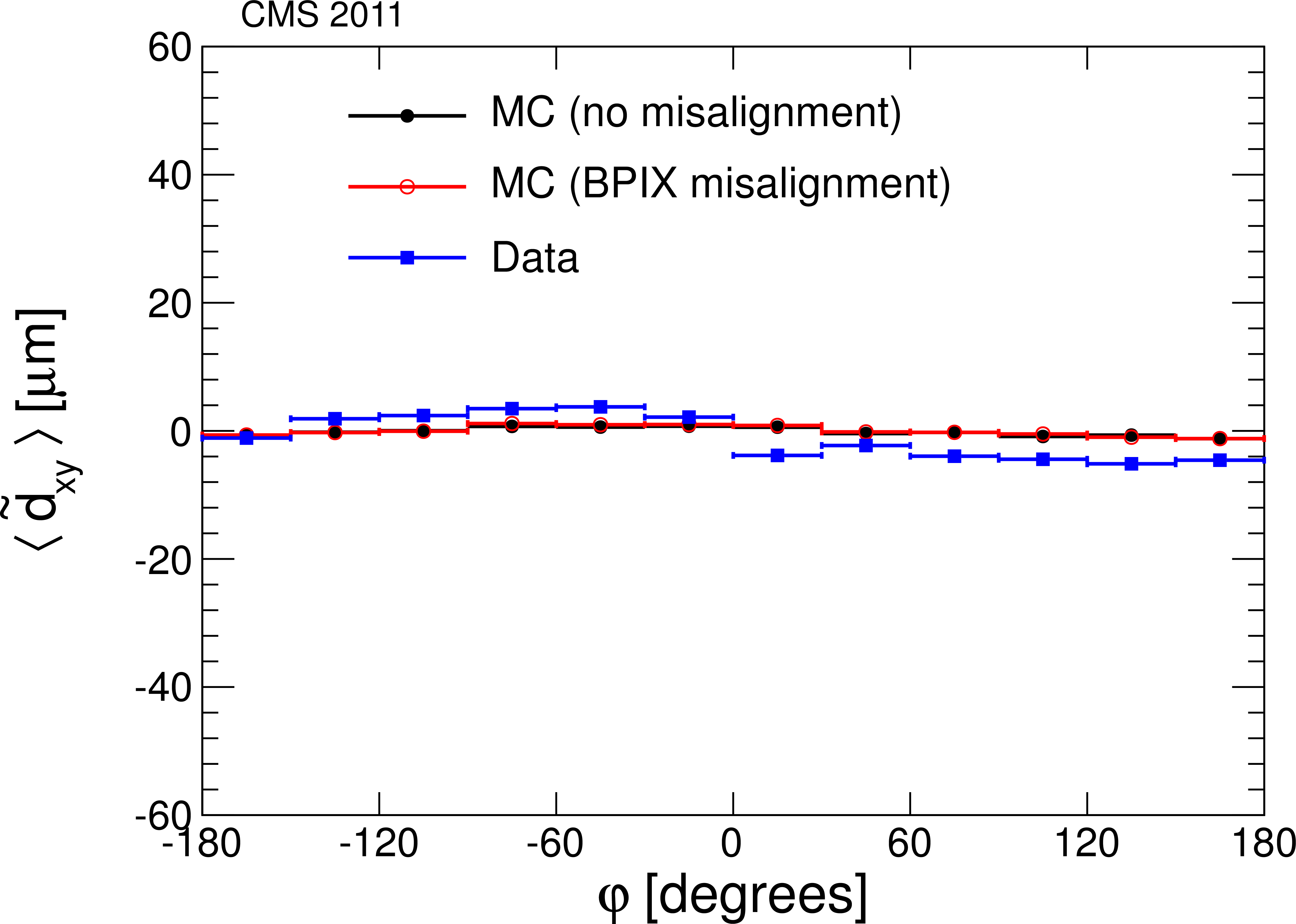
Figure 6-a:
Means of the distributions of the unbiased transverse (a) and longitudinal (b) track-vertex residuals as a function of the azimuthal angle of the track. Blue squares show the distribution obtained from about ten thousand minimum bias events recorded in 2011. Full circles show the prediction by using a simulation with perfect alignment. Open red circles show the same prediction by using a geometry with the two BPIX half-shells shifted by 20 $\mu$m in opposite $z$-directions in the simulation. |

png pdf |
Figure 6-b:
Means of the distributions of the unbiased transverse (a) and longitudinal (b) track-vertex residuals as a function of the azimuthal angle of the track. Blue squares show the distribution obtained from about ten thousand minimum bias events recorded in 2011. Full circles show the prediction by using a simulation with perfect alignment. Open red circles show the same prediction by using a geometry with the two BPIX half-shells shifted by 20 $\mu$m in opposite $z$-directions in the simulation. |

png pdf |
Figure 7:
Daily evolution of the relative longitudinal shift between the two half-shells of the BPIX as measured with the primary-vertex residuals. The open circles show the shift observed by using prompt reconstruction data in 2011. The same events were reconstructed again after the 2011 alignment campaign, which accounts for the major changes in the positions of the half-shells (shown as filled squares). Dashed vertical lines indicate the chosen IOVs boundaries where a different alignment of the pixel layers has been performed. |
png pdf |
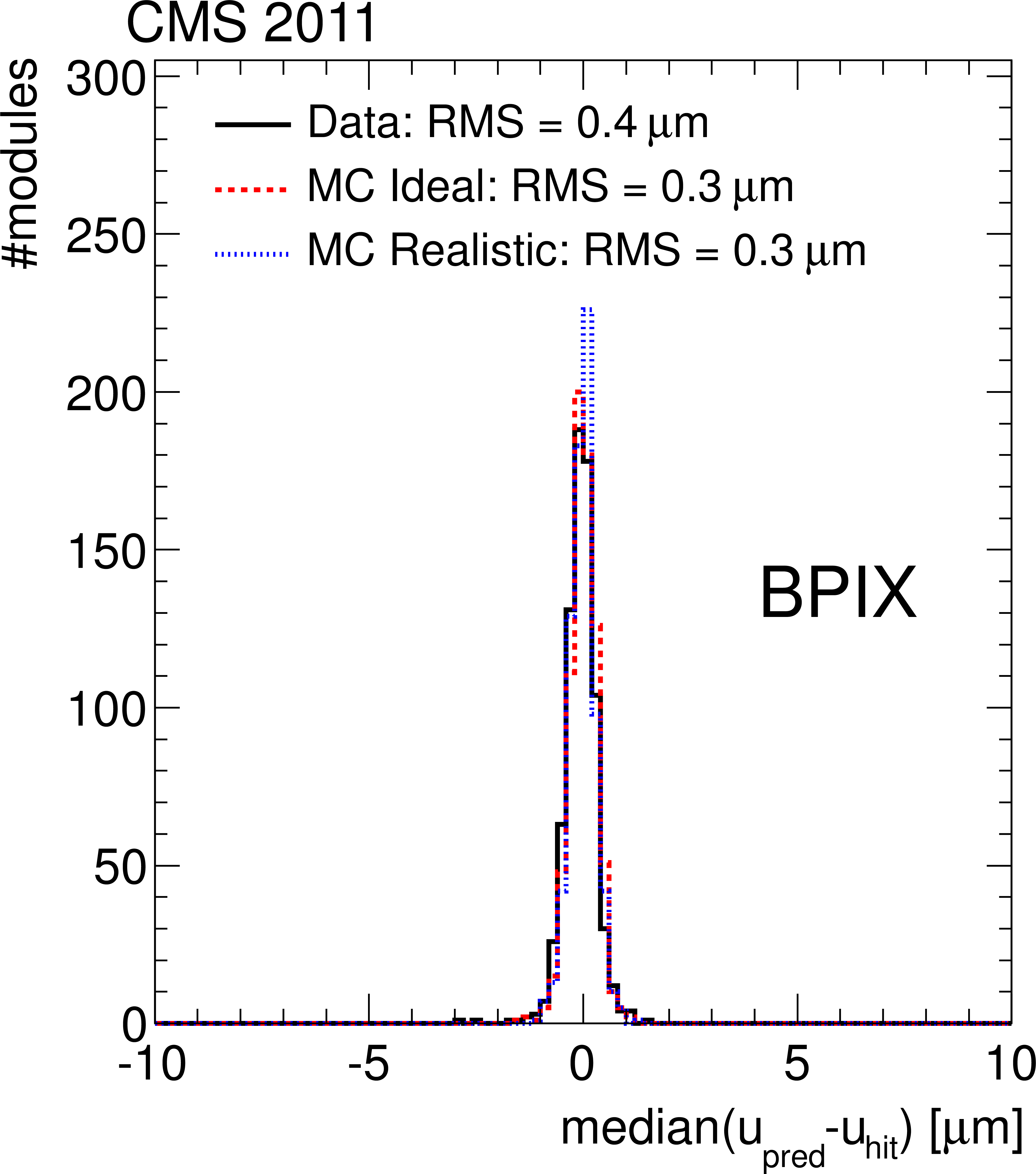
Figure 8-a:
Distributions of the medians of the residuals, for the pixel tracker barrel (a, b) and endcap modules (c, d) in $u$ (a, c) and $v$ (b, d) coordinates. Shown in each case are the distributions after alignment with 2011 data (solid line), in comparison with simulations without any misalignment (dashed line) and with realistic misalignment (dotted line). |

png pdf |
Figure 8-b:
Distributions of the medians of the residuals, for the pixel tracker barrel (a, b) and endcap modules (c, d) in $u$ (a, c) and $v$ (b, d) coordinates. Shown in each case are the distributions after alignment with 2011 data (solid line), in comparison with simulations without any misalignment (dashed line) and with realistic misalignment (dotted line). |
png pdf |
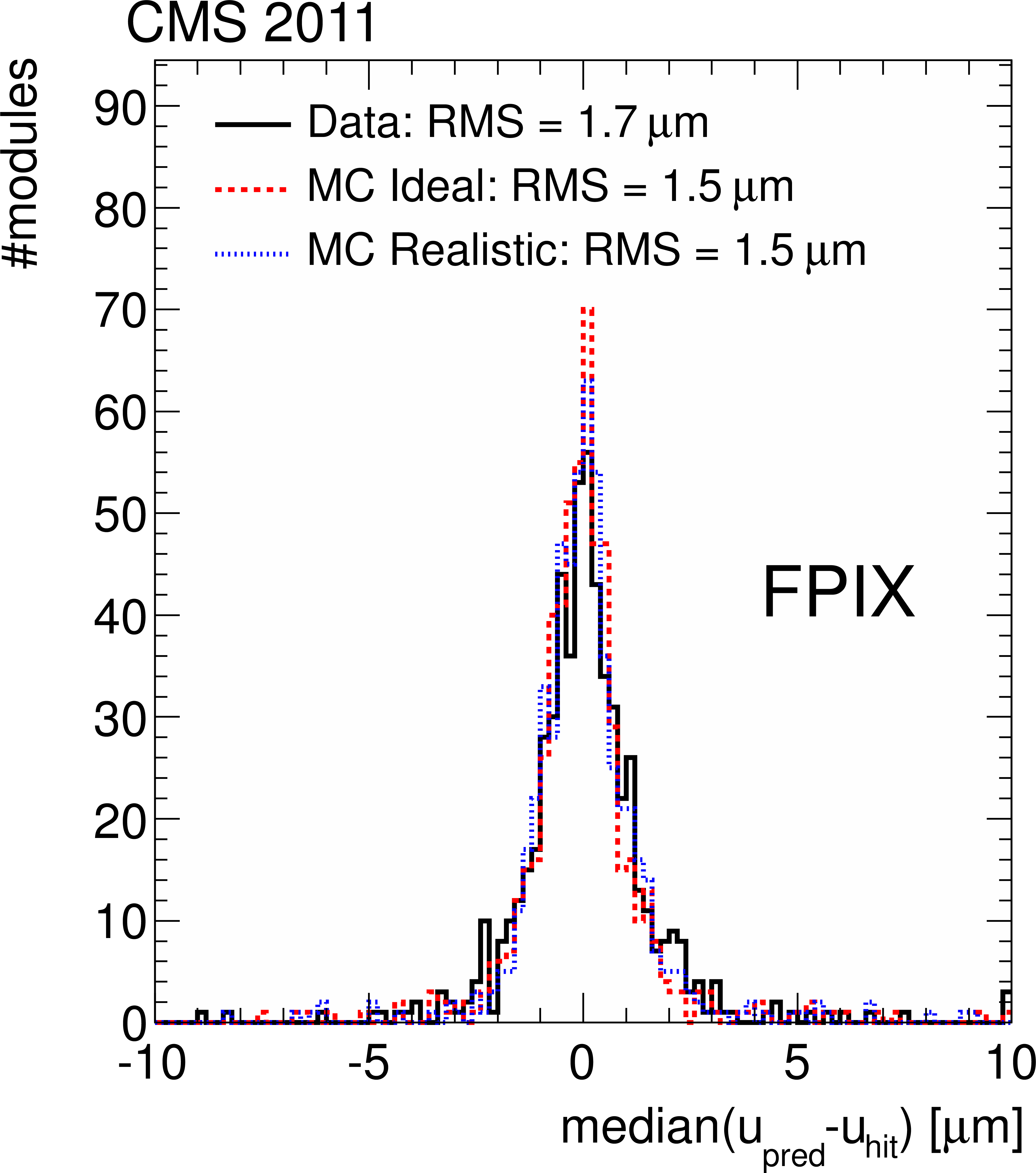
Figure 8-c:
Distributions of the medians of the residuals, for the pixel tracker barrel (a, b) and endcap modules (c, d) in $u$ (a, c) and $v$ (b, d) coordinates. Shown in each case are the distributions after alignment with 2011 data (solid line), in comparison with simulations without any misalignment (dashed line) and with realistic misalignment (dotted line). |
png pdf |
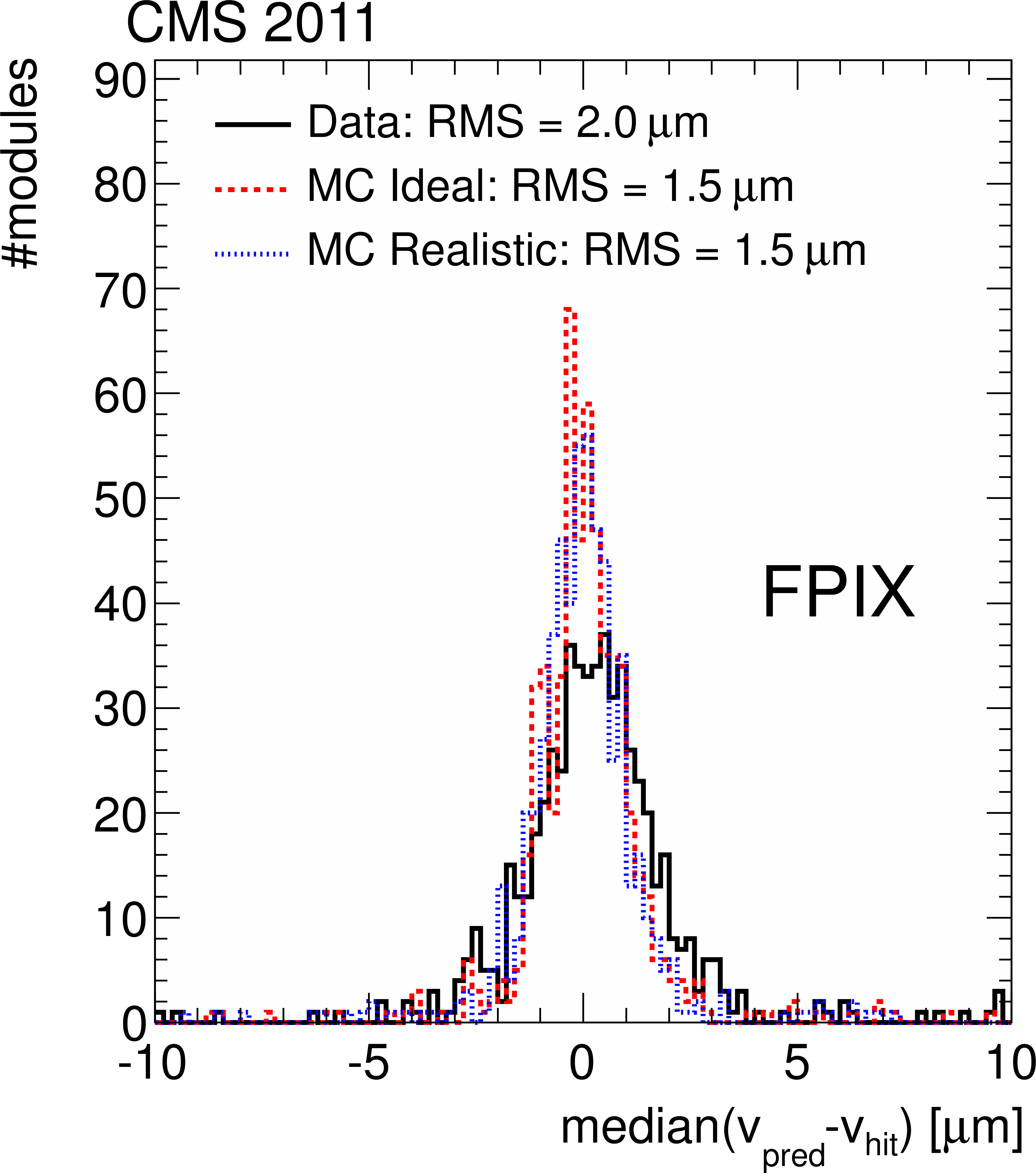
Figure 8-d:
Distributions of the medians of the residuals, for the pixel tracker barrel (a, b) and endcap modules (c, d) in $u$ (a, c) and $v$ (b, d) coordinates. Shown in each case are the distributions after alignment with 2011 data (solid line), in comparison with simulations without any misalignment (dashed line) and with realistic misalignment (dotted line). |
png pdf |
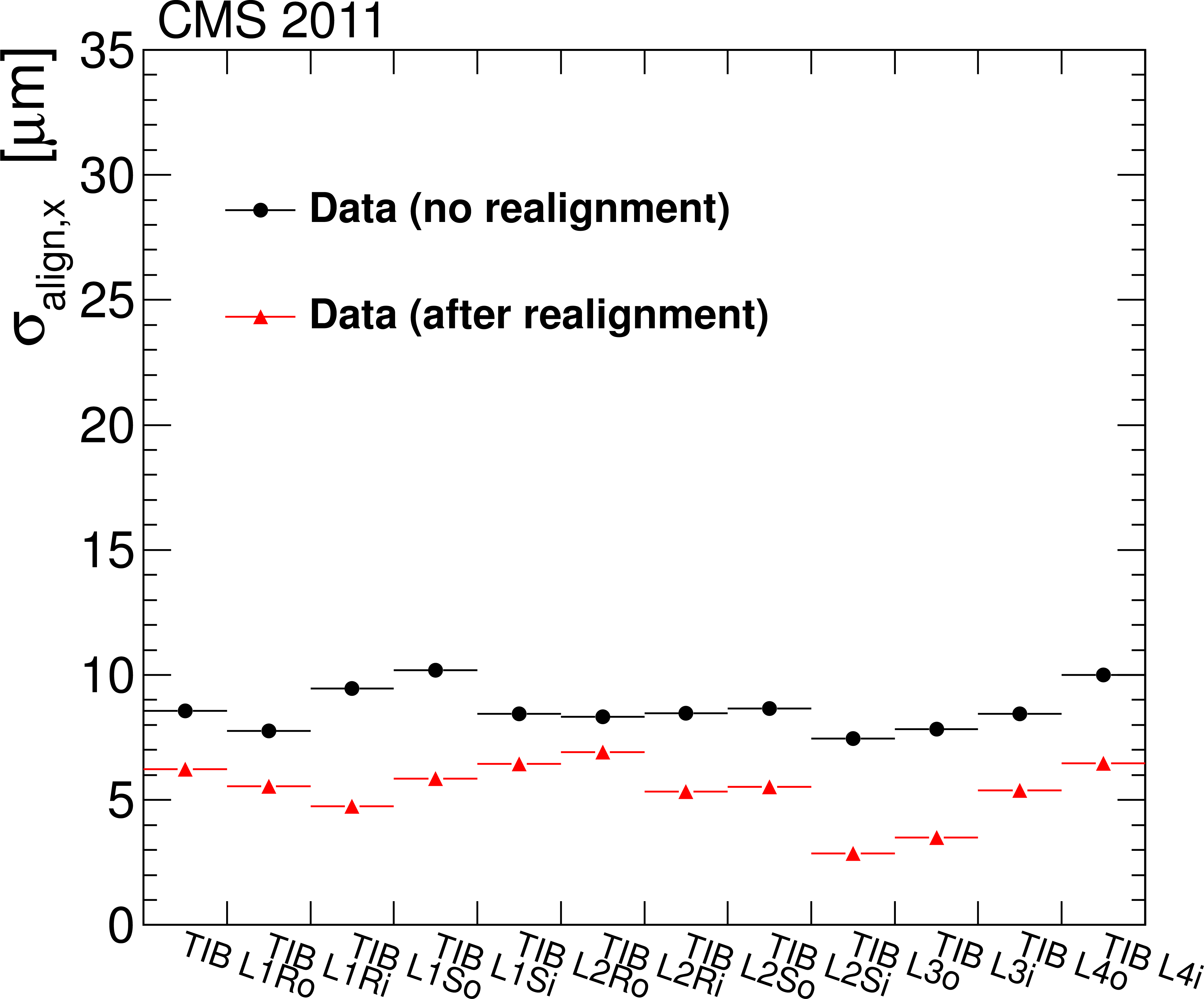
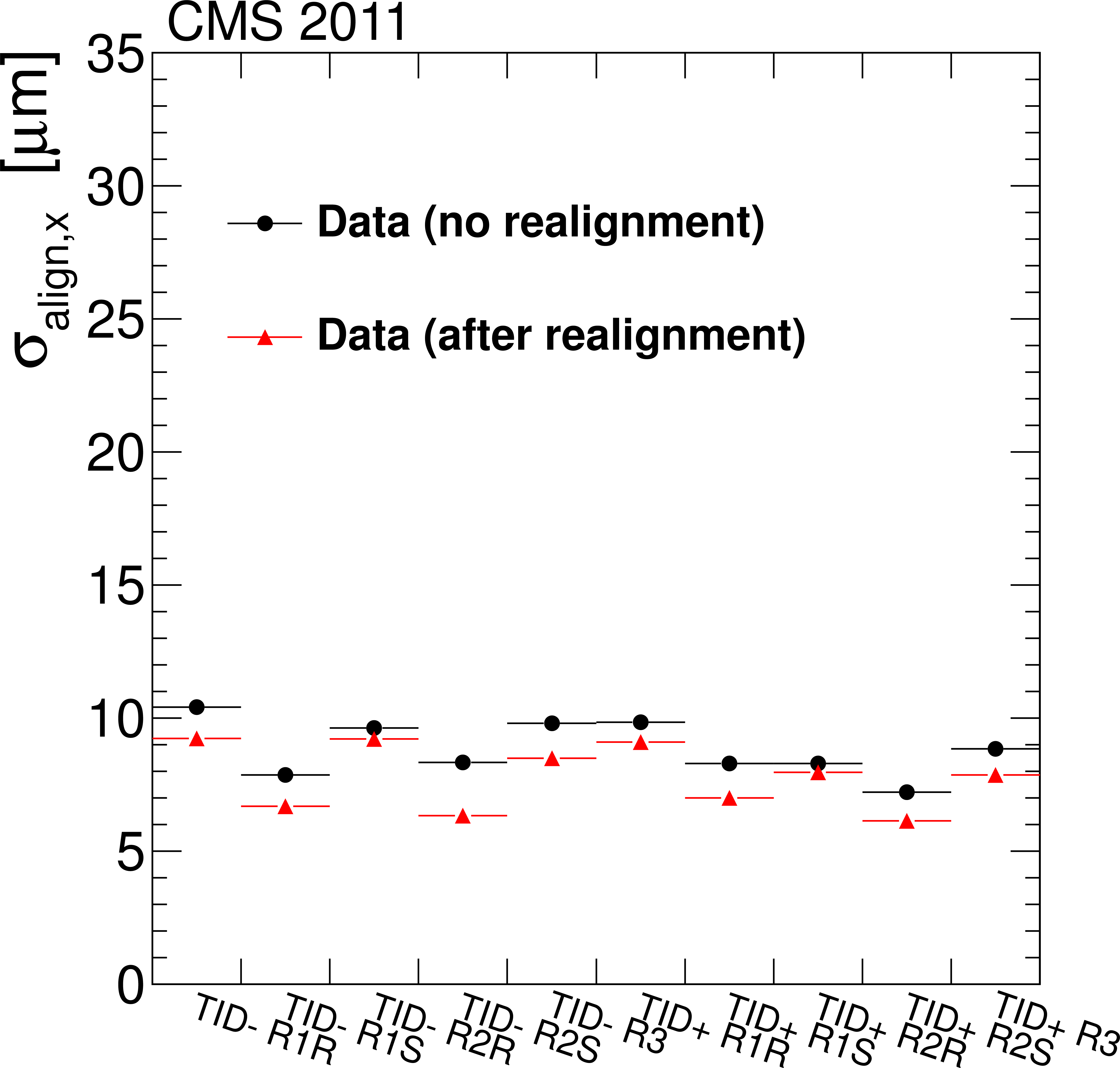
Figure 9-a:
Alignment accuracy in the subdetectors TIB, TID and TEC, determined for each sensor group, with the normalised residuals method. The black dots show the alignment accuracy before the dedicated alignment with the 2011 data, with the older alignment constants used in the prompt reconstruction, while the red triangles are obtained with the dedicated alignment applied in the reprocessing of the data. |
png pdf |
Figure 9-b:
Alignment accuracy in the subdetectors TIB, TID and TEC, determined for each sensor group, with the normalised residuals method. The black dots show the alignment accuracy before the dedicated alignment with the 2011 data, with the older alignment constants used in the prompt reconstruction, while the red triangles are obtained with the dedicated alignment applied in the reprocessing of the data. |

png pdf |
Figure 9-c:
Alignment accuracy in the subdetectors TIB, TID and TEC, determined for each sensor group, with the normalised residuals method. The black dots show the alignment accuracy before the dedicated alignment with the 2011 data, with the older alignment constants used in the prompt reconstruction, while the red triangles are obtained with the dedicated alignment applied in the reprocessing of the data. |
png pdf |
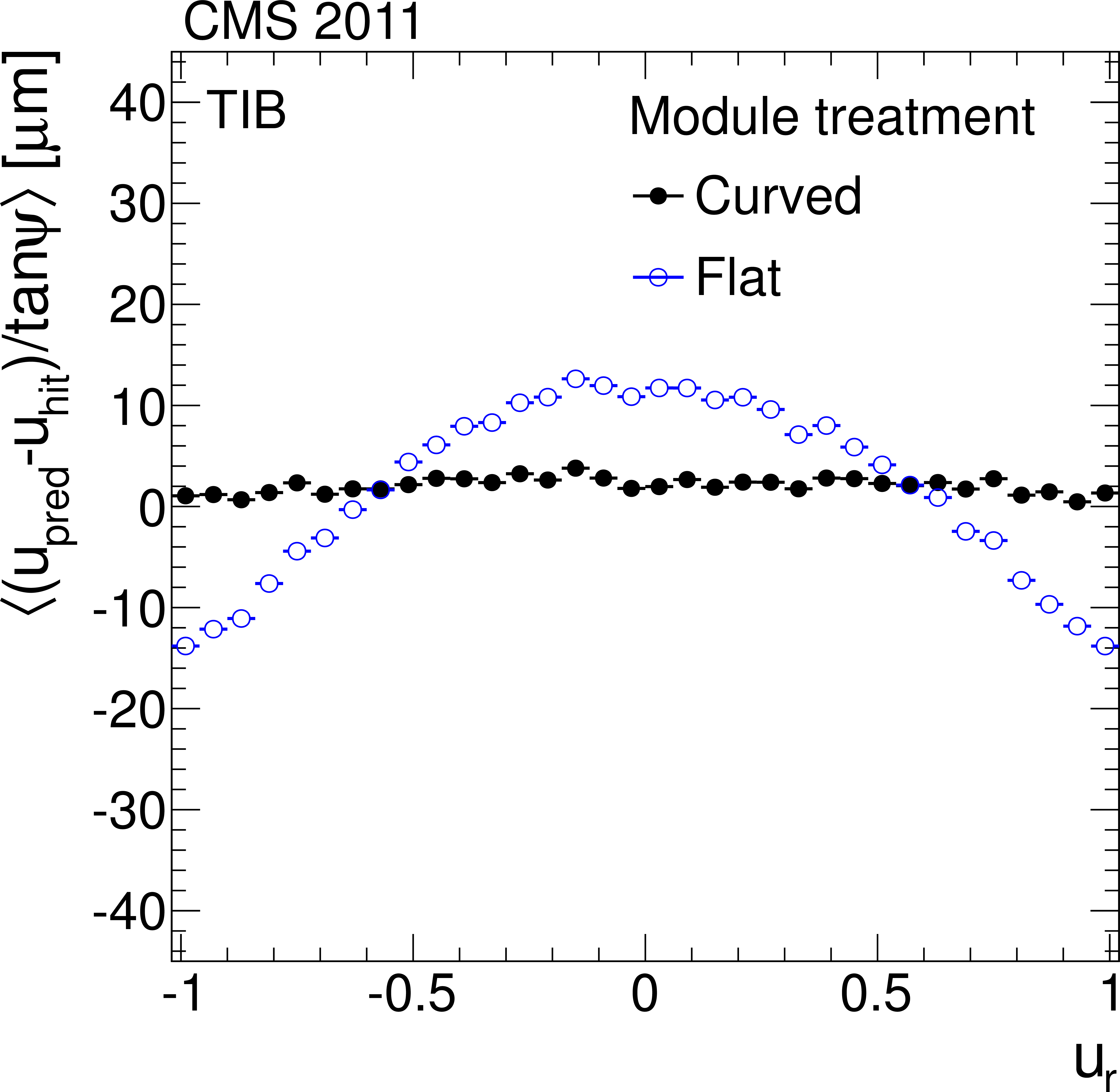
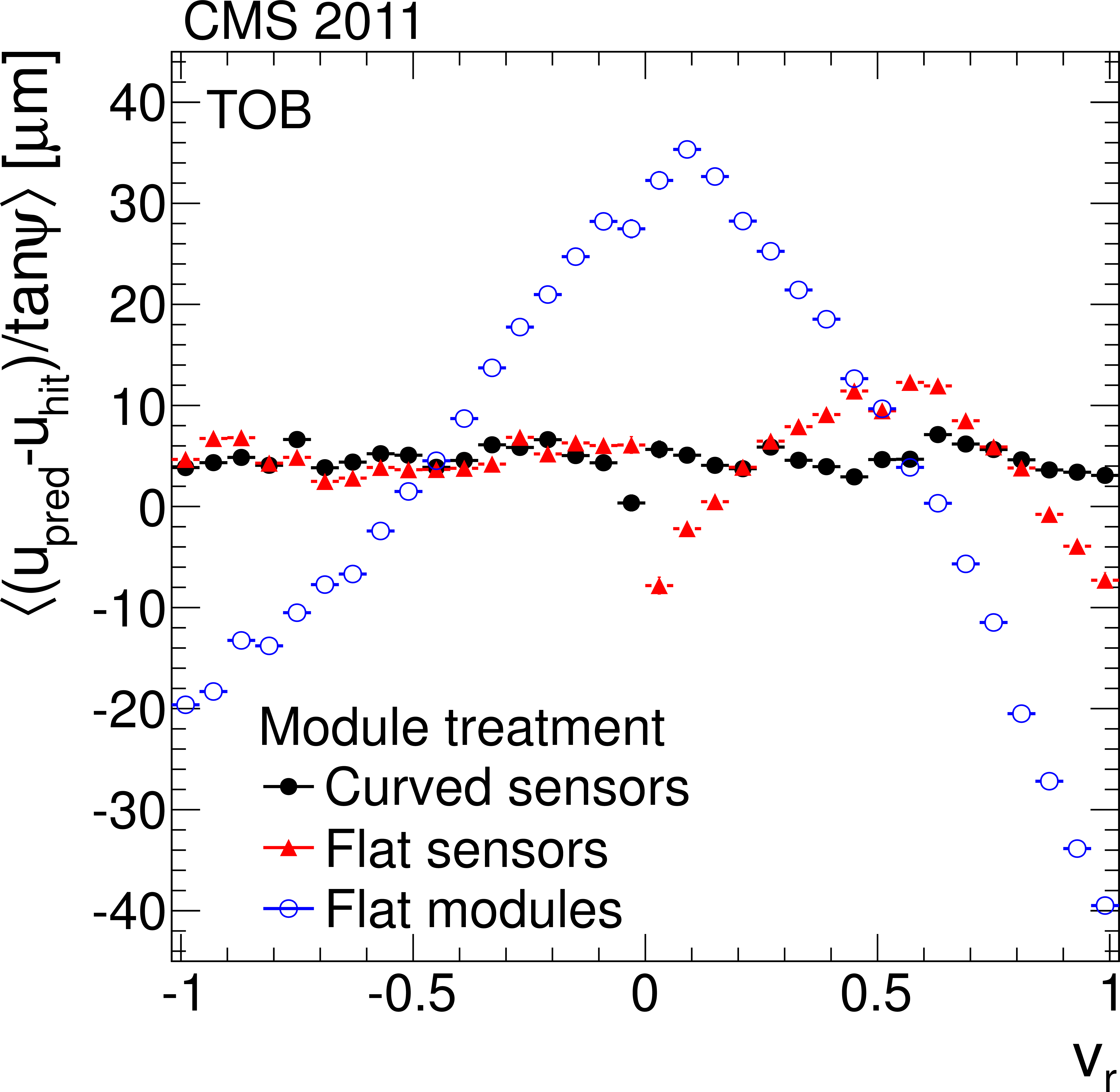
Figure 10-a:
Distributions of the average weighted means of the $\Delta w = \Delta u / \tan\psi $ track-hit residuals as a function of the relative positions of cosmic ray tracks on the modules along the local $u$- (a, c, e) and $v$-axis (b, d, f) for different approaches to parameterise the module shape. The (a, b) and (c, d) plots show the average for all the TIB and TOB modules, respectively, and the (e, f) plots show the double-sensor modules of the rings 5-7 of the TEC. Each residual is weighted by $\tan^2\psi $ of the track. |

png pdf |
Figure 10-b:
Distributions of the average weighted means of the $\Delta w = \Delta u / \tan\psi $ track-hit residuals as a function of the relative positions of cosmic ray tracks on the modules along the local $u$- (a, c, e) and $v$-axis (b, d, f) for different approaches to parameterise the module shape. The (a, b) and (c, d) plots show the average for all the TIB and TOB modules, respectively, and the (e, f) plots show the double-sensor modules of the rings 5-7 of the TEC. Each residual is weighted by $\tan^2\psi $ of the track. |
png pdf |
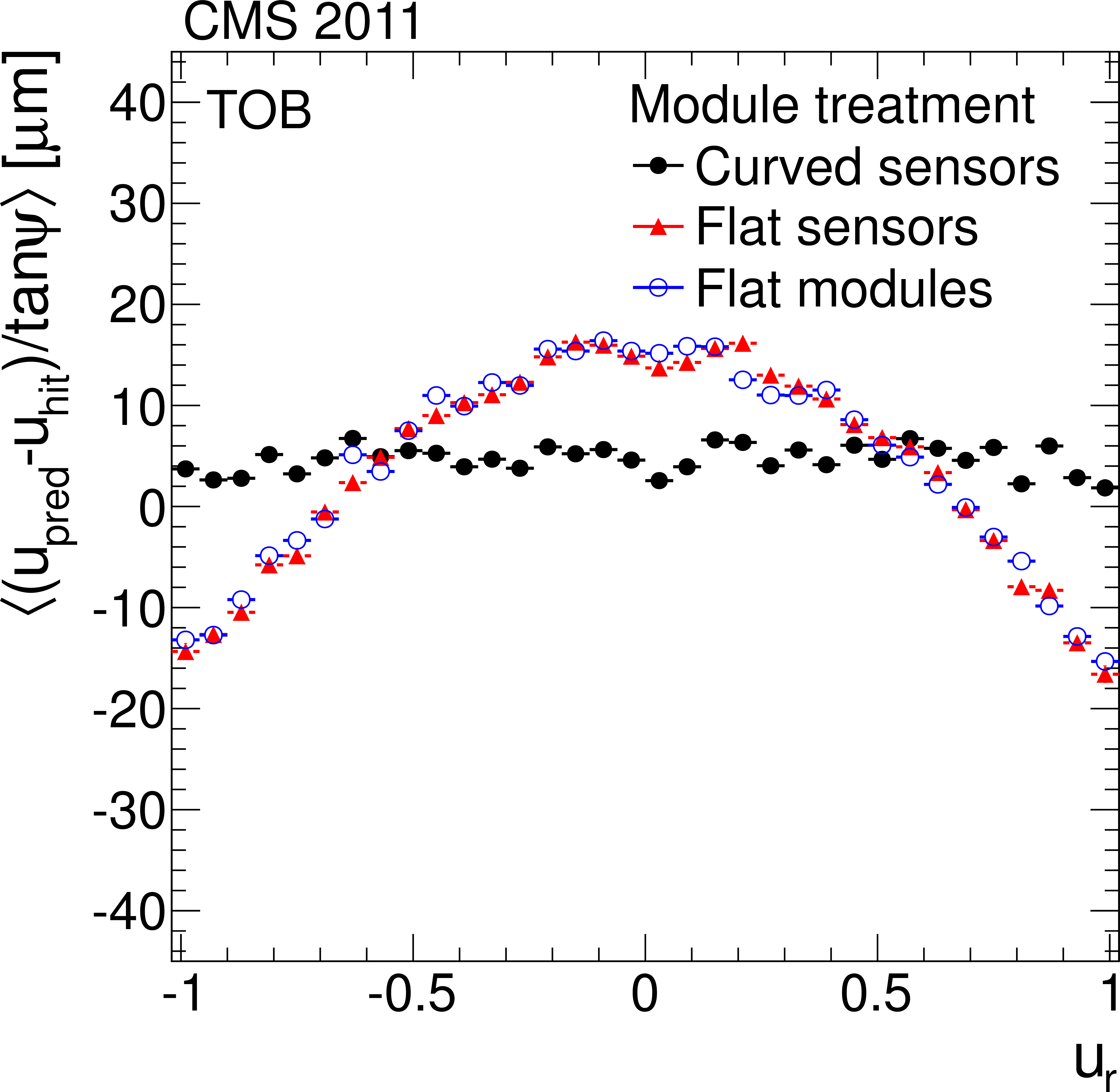
Figure 10-c:
Distributions of the average weighted means of the $\Delta w = \Delta u / \tan\psi $ track-hit residuals as a function of the relative positions of cosmic ray tracks on the modules along the local $u$- (a, c, e) and $v$-axis (b, d, f) for different approaches to parameterise the module shape. The (a, b) and (c, d) plots show the average for all the TIB and TOB modules, respectively, and the (e, f) plots show the double-sensor modules of the rings 5-7 of the TEC. Each residual is weighted by $\tan^2\psi $ of the track. |
png pdf |
Figure 10-d:
Distributions of the average weighted means of the $\Delta w = \Delta u / \tan\psi $ track-hit residuals as a function of the relative positions of cosmic ray tracks on the modules along the local $u$- (a, c, e) and $v$-axis (b, d, f) for different approaches to parameterise the module shape. The (a, b) and (c, d) plots show the average for all the TIB and TOB modules, respectively, and the (e, f) plots show the double-sensor modules of the rings 5-7 of the TEC. Each residual is weighted by $\tan^2\psi $ of the track. |
png pdf |
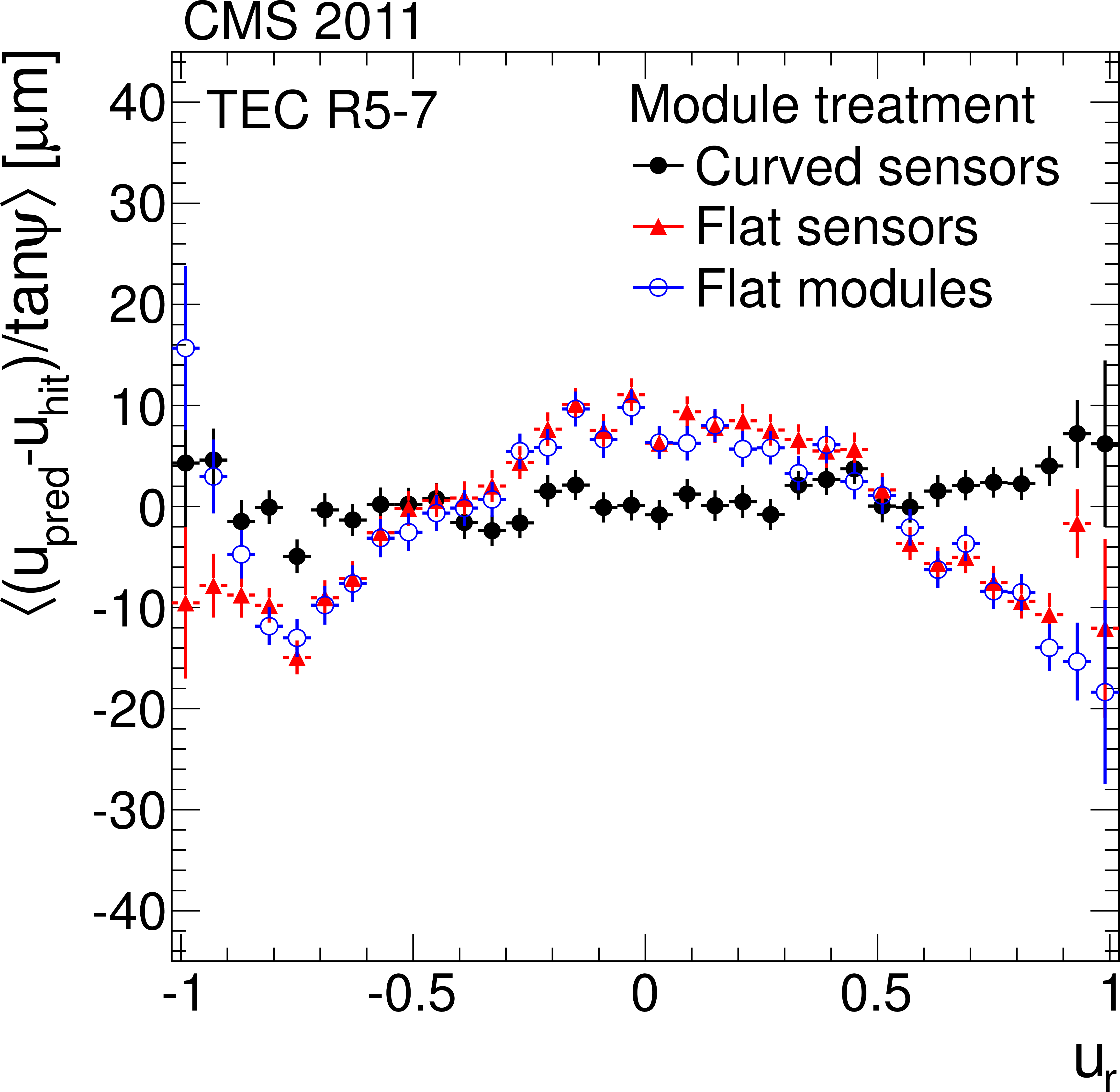
Figure 10-e:
Distributions of the average weighted means of the $\Delta w = \Delta u / \tan\psi $ track-hit residuals as a function of the relative positions of cosmic ray tracks on the modules along the local $u$- (a, c, e) and $v$-axis (b, d, f) for different approaches to parameterise the module shape. The (a, b) and (c, d) plots show the average for all the TIB and TOB modules, respectively, and the (e, f) plots show the double-sensor modules of the rings 5-7 of the TEC. Each residual is weighted by $\tan^2\psi $ of the track. |
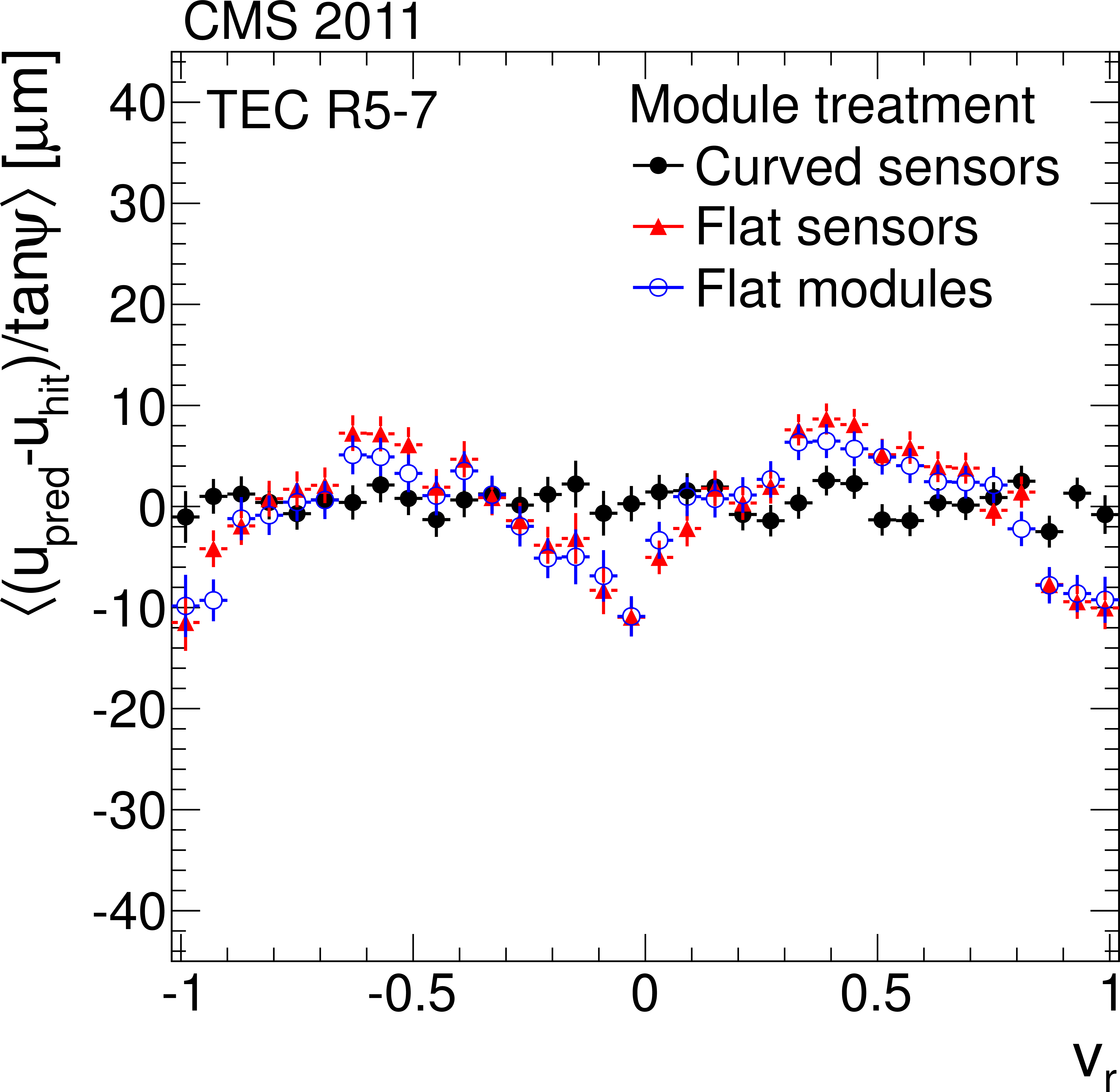
png pdf |
Figure 10-f:
Distributions of the average weighted means of the $\Delta w = \Delta u / \tan\psi $ track-hit residuals as a function of the relative positions of cosmic ray tracks on the modules along the local $u$- (a, c, e) and $v$-axis (b, d, f) for different approaches to parameterise the module shape. The (a, b) and (c, d) plots show the average for all the TIB and TOB modules, respectively, and the (e, f) plots show the double-sensor modules of the rings 5-7 of the TEC. Each residual is weighted by $\tan^2\psi $ of the track. |
png pdf |
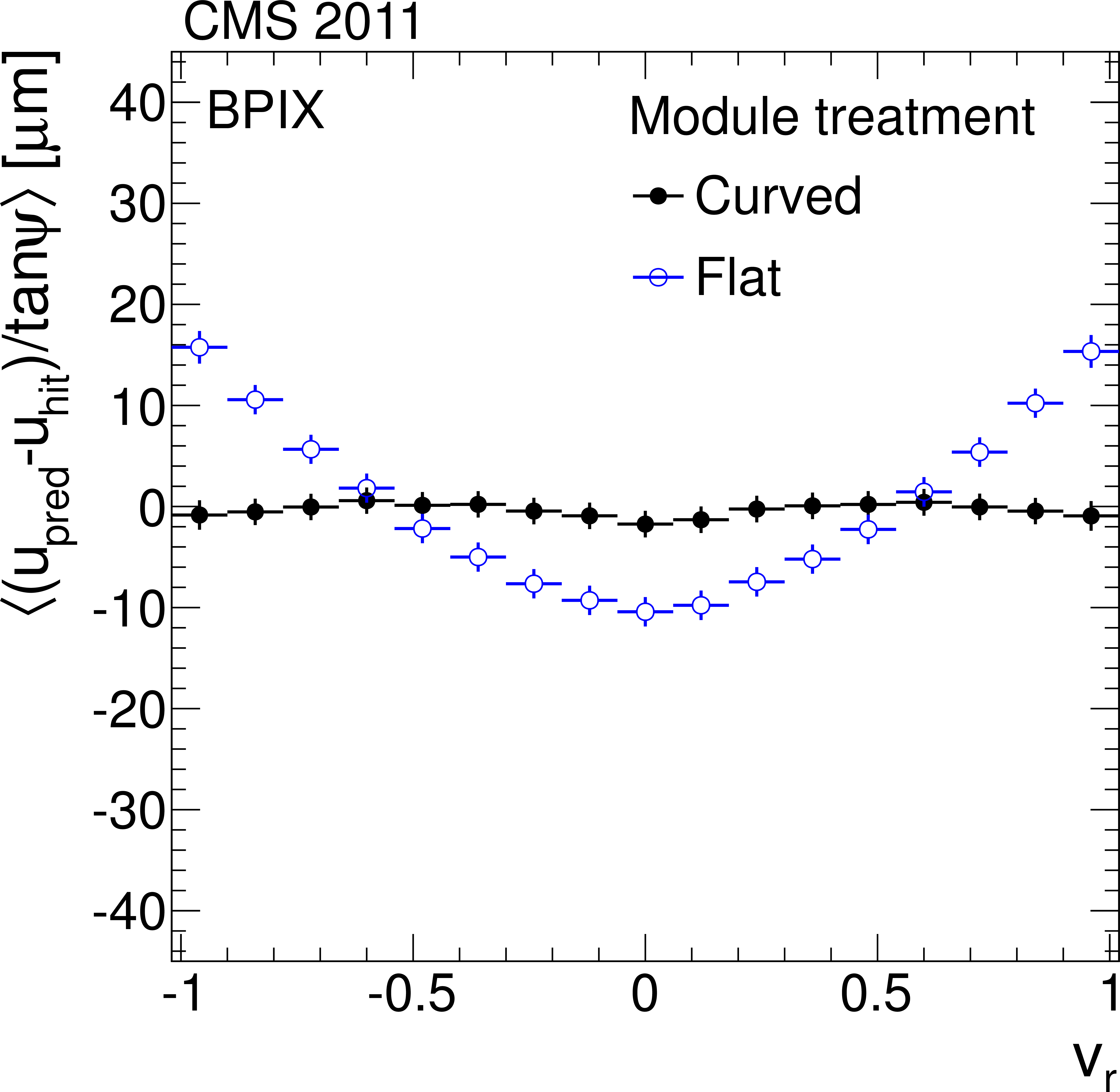
Figure 11-a:
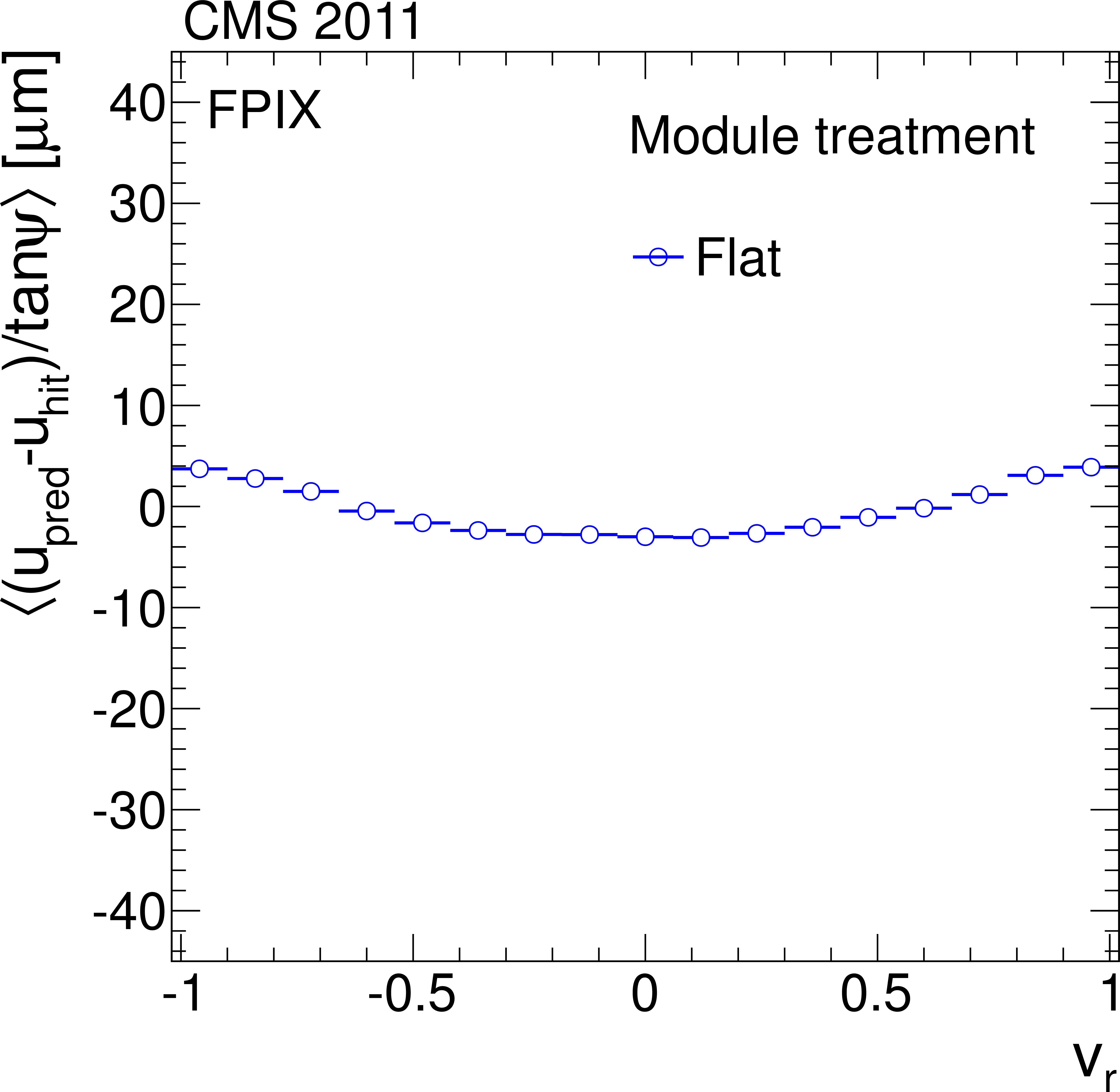
Distributions of the average weighted means of the $\Delta w = \Delta u/\tan\psi $ track-hit residuals as a function of the relative positions of tracks from proton-proton collisions on the modules along the local $v$-axis for different approaches to parameterise the module shapes. The a plot shows the BPIX and the b one the FPIX. Each residual is weighted by $\tan^2\psi $ of the track. |
png pdf |
Figure 11-b:
Distributions of the average weighted means of the $\Delta w = \Delta u/\tan\psi $ track-hit residuals as a function of the relative positions of tracks from proton-proton collisions on the modules along the local $v$-axis for different approaches to parameterise the module shapes. The a plot shows the BPIX and the b one the FPIX. Each residual is weighted by $\tan^2\psi $ of the track. |
png pdf |
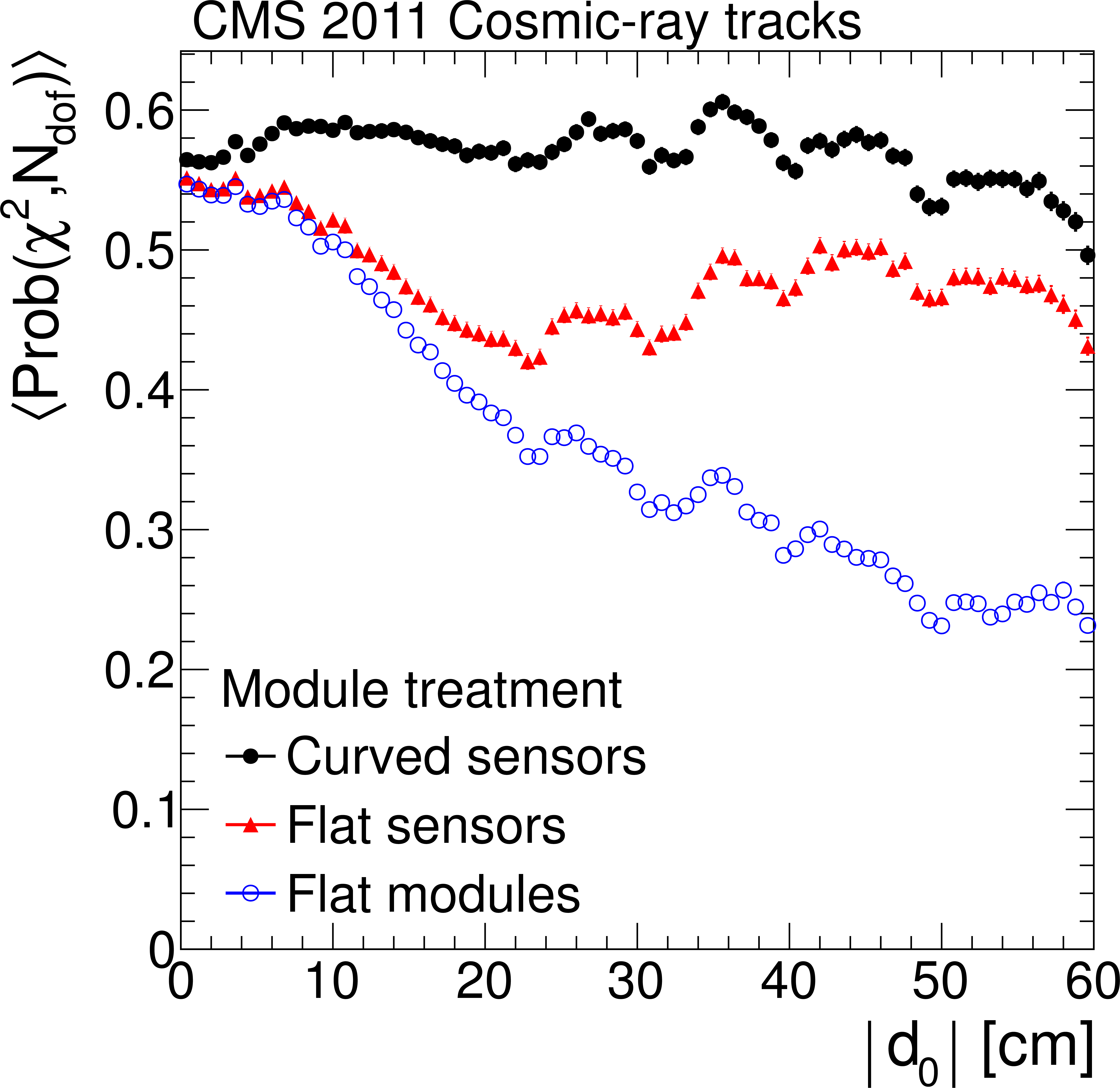
Figure 12:
Mean probability $< \text {Prob}(\chi ^2,{N_\mathrm {dof}}) > $ of cosmic ray track fits as a function of their distance of closest approach to the nominal beam line for the different approaches to parameterise the module shapes. |
png pdf |
Figure 13-a:
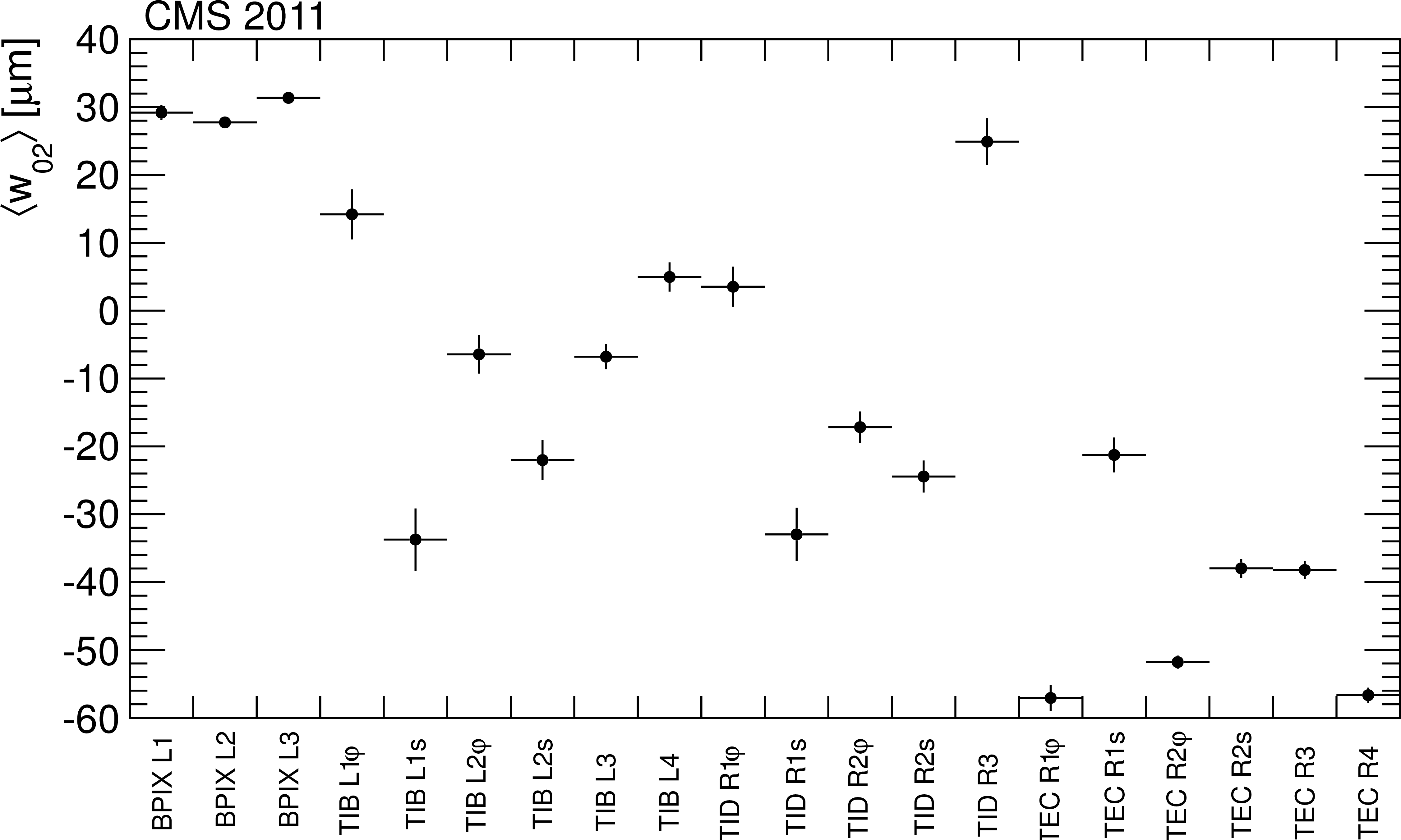
Sensor curvatures along the local $u$ (a, b) and $v$ (c, d) coordinate for single- (a, c) and double-sensor (b, d) modules, averaged over layers (L) and rings (R), respectively. Stereo (s) and $r\varphi $ ($\varphi $) modules within a layer or ring are separated. |

png pdf |
Figure 13-b:
Sensor curvatures along the local $u$ (a, b) and $v$ (c, d) coordinate for single- (a, c) and double-sensor (b, d) modules, averaged over layers (L) and rings (R), respectively. Stereo (s) and $r\varphi $ ($\varphi $) modules within a layer or ring are separated. |
png pdf |
Figure 13-c:
Sensor curvatures along the local $u$ (a, b) and $v$ (c, d) coordinate for single- (a, c) and double-sensor (b, d) modules, averaged over layers (L) and rings (R), respectively. Stereo (s) and $r\varphi $ ($\varphi $) modules within a layer or ring are separated. |

png pdf |
Figure 13-d:
Sensor curvatures along the local $u$ (a, b) and $v$ (c, d) coordinate for single- (a, c) and double-sensor (b, d) modules, averaged over layers (L) and rings (R), respectively. Stereo (s) and $r\varphi $ ($\varphi $) modules within a layer or ring are separated. |

png pdf |
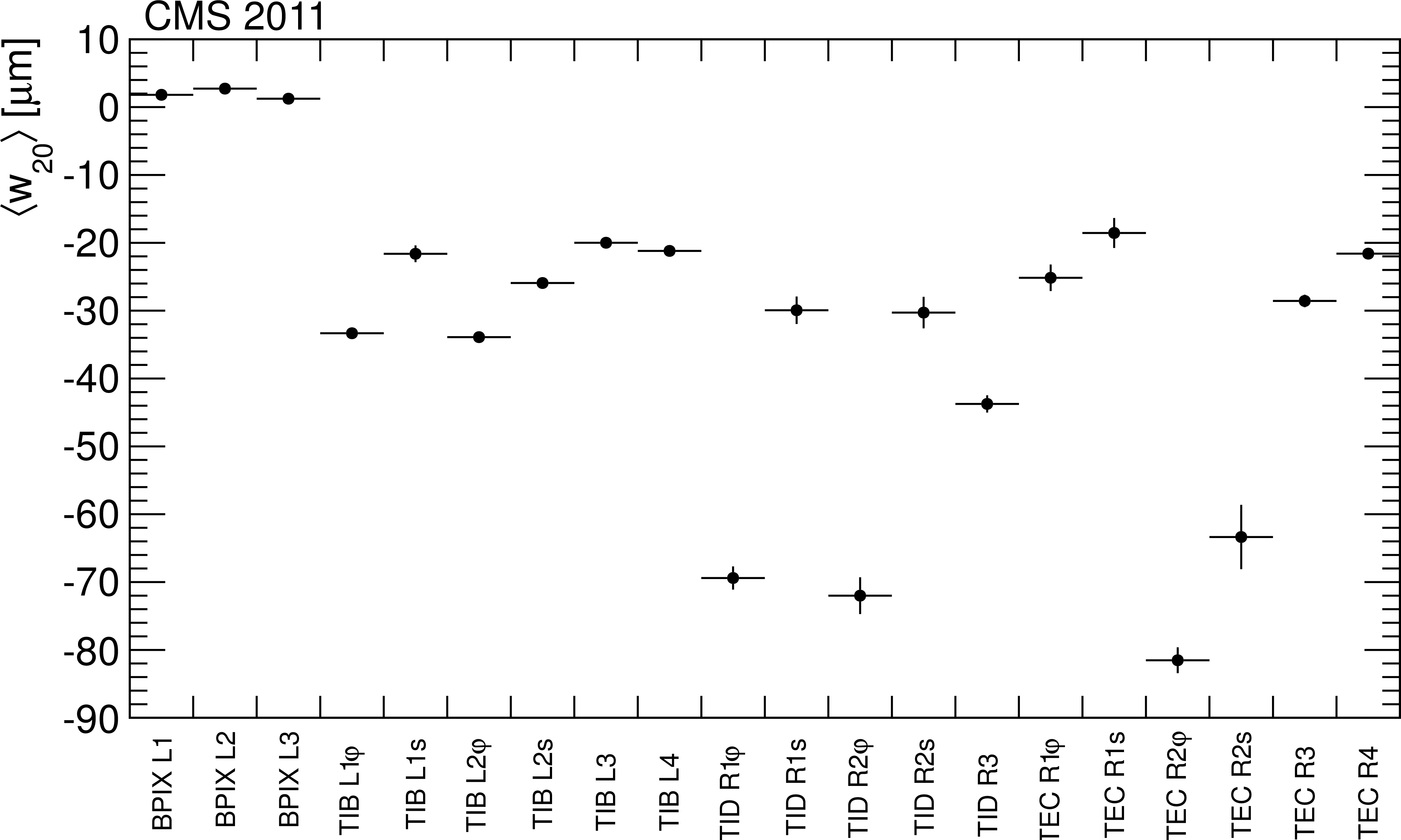
Figure 14:
Kink angle $\Delta \alpha $ for double-sensor modules, averaged over layers (L) and rings (R), respectively. Stereo (s) and $r\varphi $ ($\varphi $) modules within the same layer or ring are separated. |

png pdf |
Figure 15:
Distributions of the kink angles $\Delta \alpha $ and $\Delta \beta $ of TOB modules. |
png pdf |
Figure 16-a:
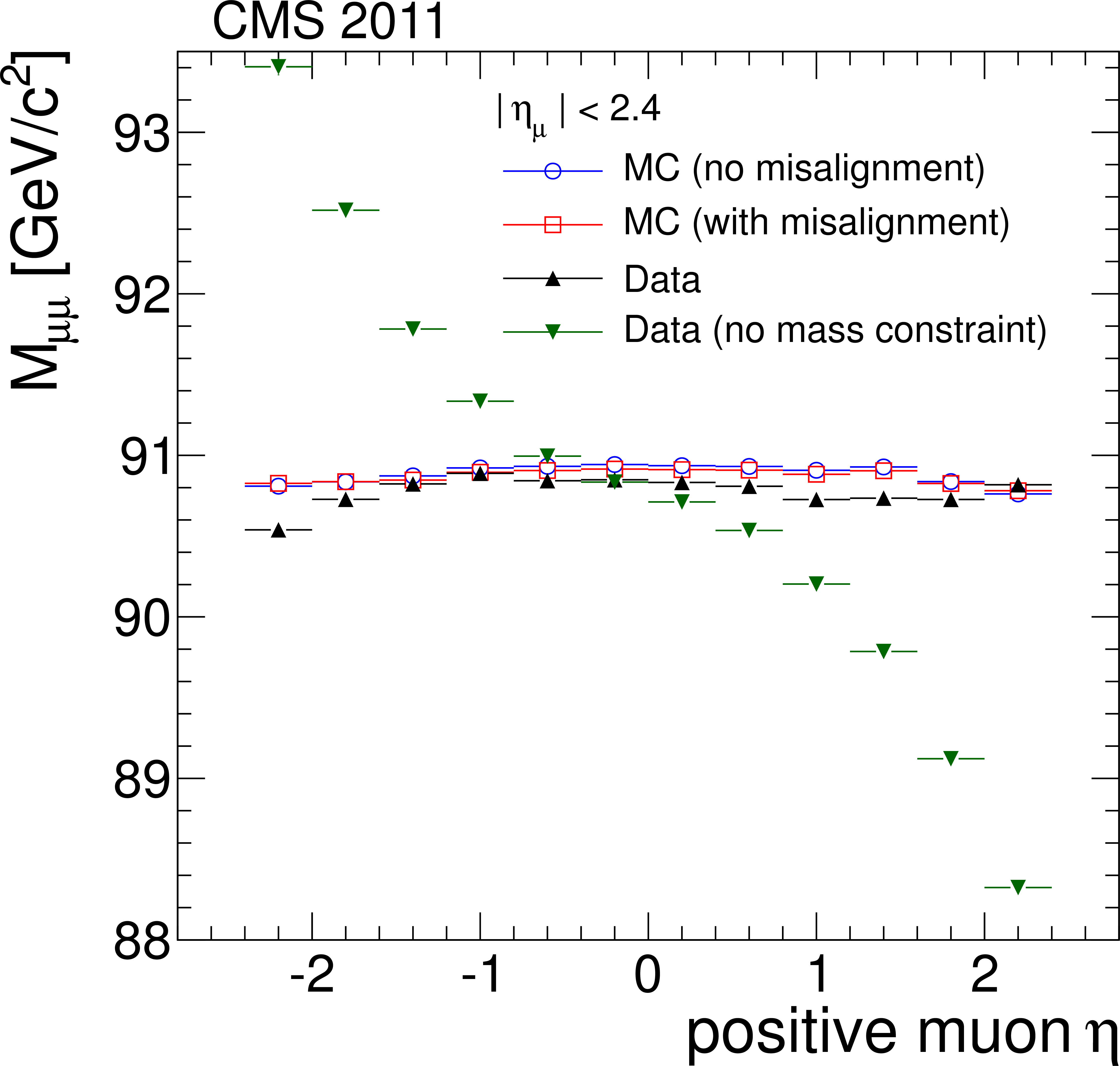
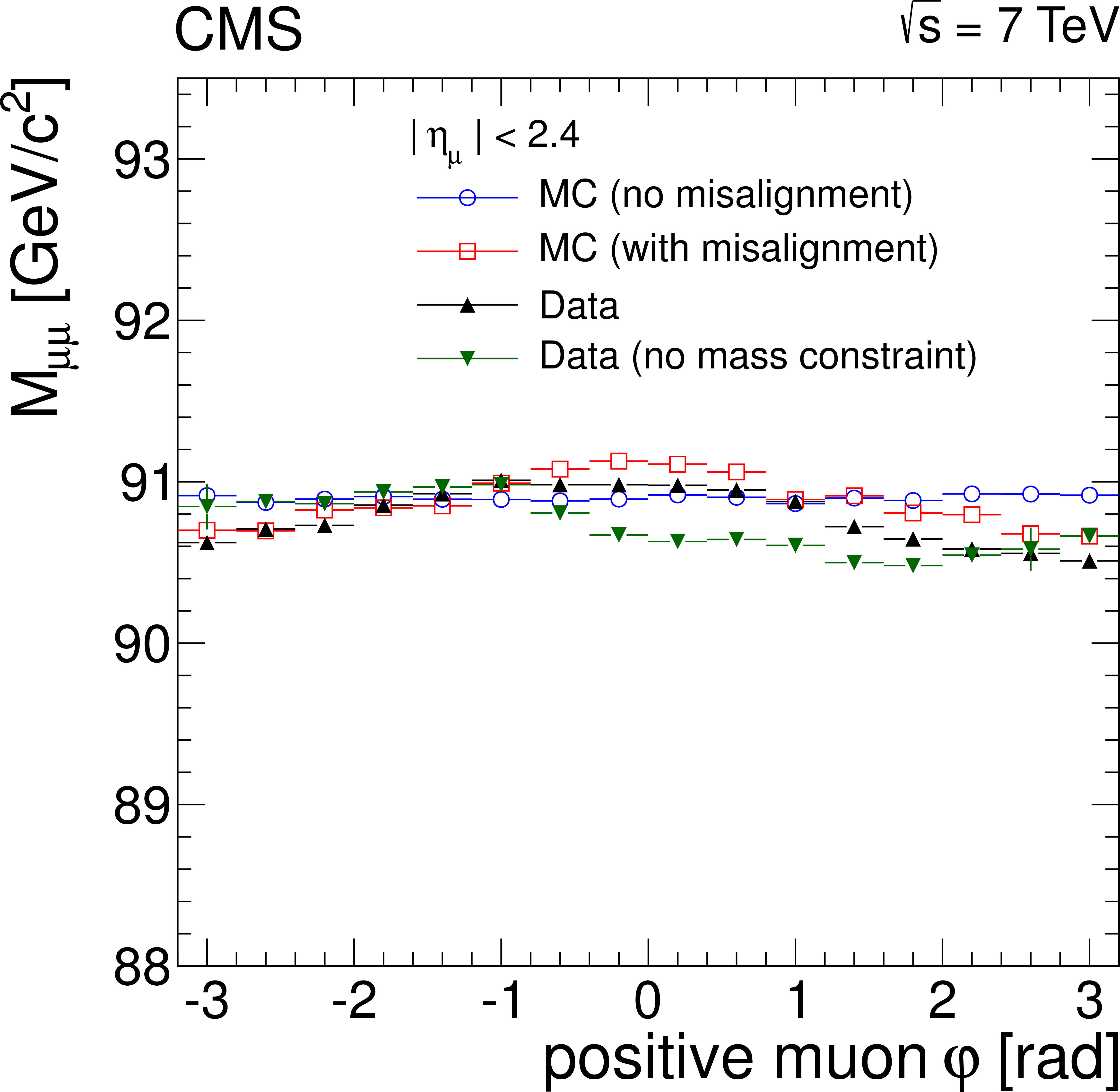
Invariant mass of $ {\mathrm {Z}} \to \mu ^+\mu ^-$ candidates as a function of $\eta $ (a) and $\varphi $ (b) of the positively charged muon. Distributions from aligned data are shown as black upward-pointing triangles. Distributions from a simulation without misalignment and with realistic misalignment (see section Strategy) are presented as blue hollow circles and red hollow markers, respectively. The same distribution with the data but with a geometry produced without using the Z-boson mass information is presented with green downward-pointing triangles. |
png pdf |
Figure 16-b:
Invariant mass of $ {\mathrm {Z}} \to \mu ^+\mu ^-$ candidates as a function of $\eta $ (a) and $\varphi $ (b) of the positively charged muon. Distributions from aligned data are shown as black upward-pointing triangles. Distributions from a simulation without misalignment and with realistic misalignment (see section Strategy) are presented as blue hollow circles and red hollow markers, respectively. The same distribution with the data but with a geometry produced without using the Z-boson mass information is presented with green downward-pointing triangles. |
png pdf |
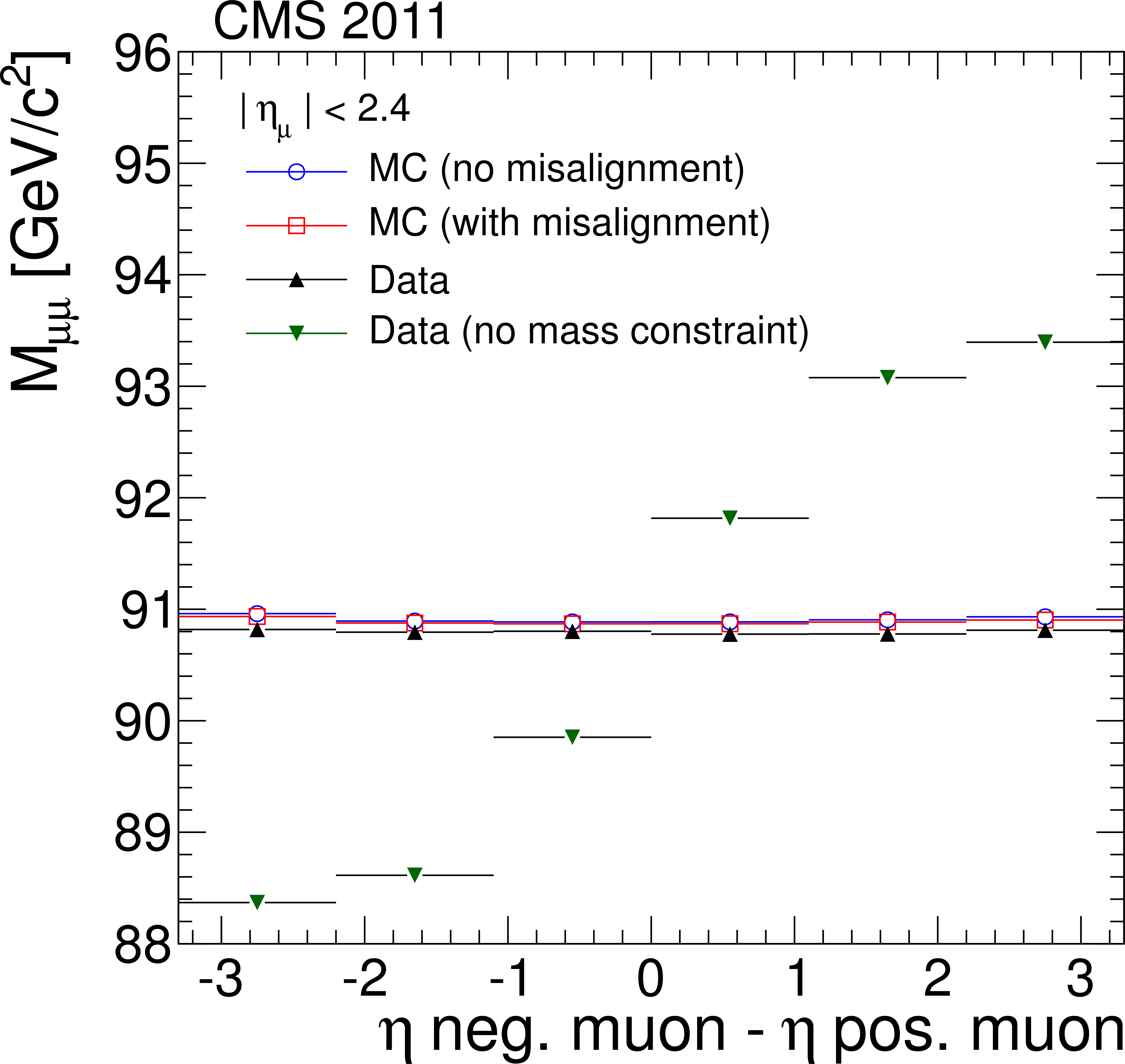
Figure 17:
Invariant mass of $ {\mathrm {Z}} \to \mu ^+\mu ^-$ candidates as a function of the $\eta $ separation of the two muons. Distributions from aligned data are shown as black upward-pointing triangles. Distributions from a simulation without misalignment and with realistic misalignment are presented as blue hollow circles and red hollow markers, respectively. The same distribution from the data but with a geometry produced without using the Z-boson mass information is presented with green downward-pointing triangles. |
png pdf |
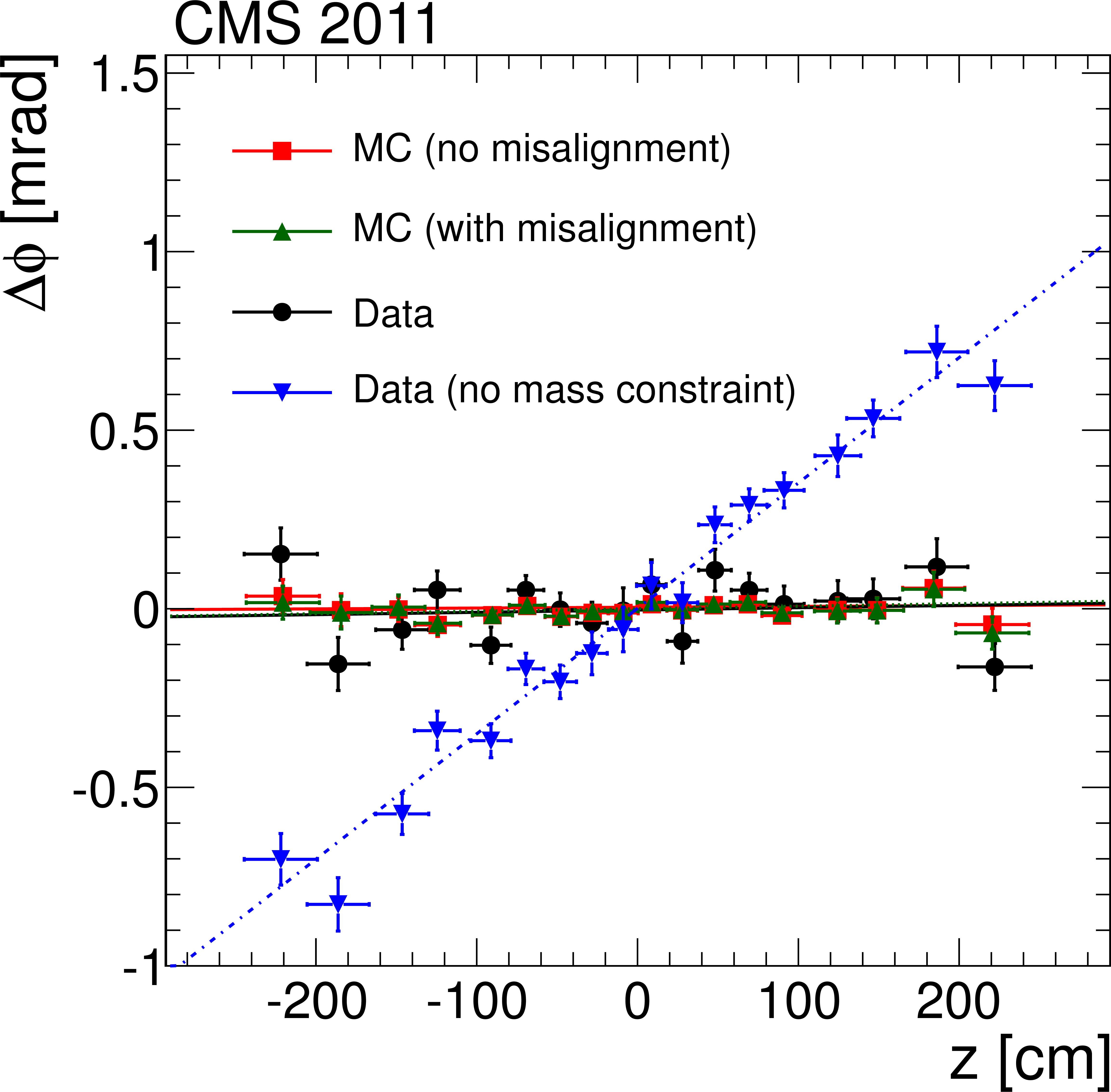
Figure 18-a:
Rotational misalignment, $\Delta \phi $, as a function of the $z$-position at $r=$ 1 m (a) and $\varphi $ (b) of the track. Distributions from 2011 data with an aligned geometry are shown as black dots. The distributions from the simulation without misalignment and with realistic misalignment are presented as red squares and green upward-pointing triangles, respectively. The blue downward-pointing triangles in the left figure show the distribution by using an alignment obtained without using the information on the Z-boson mass. |

png pdf |
Figure 18-b:
Rotational misalignment, $\Delta \phi $, as a function of the $z$-position at $r=$ 1 m (a) and $\varphi $ (b) of the track. Distributions from 2011 data with an aligned geometry are shown as black dots. The distributions from the simulation without misalignment and with realistic misalignment are presented as red squares and green upward-pointing triangles, respectively. The blue downward-pointing triangles in the left figure show the distribution by using an alignment obtained without using the information on the Z-boson mass. |
png pdf |
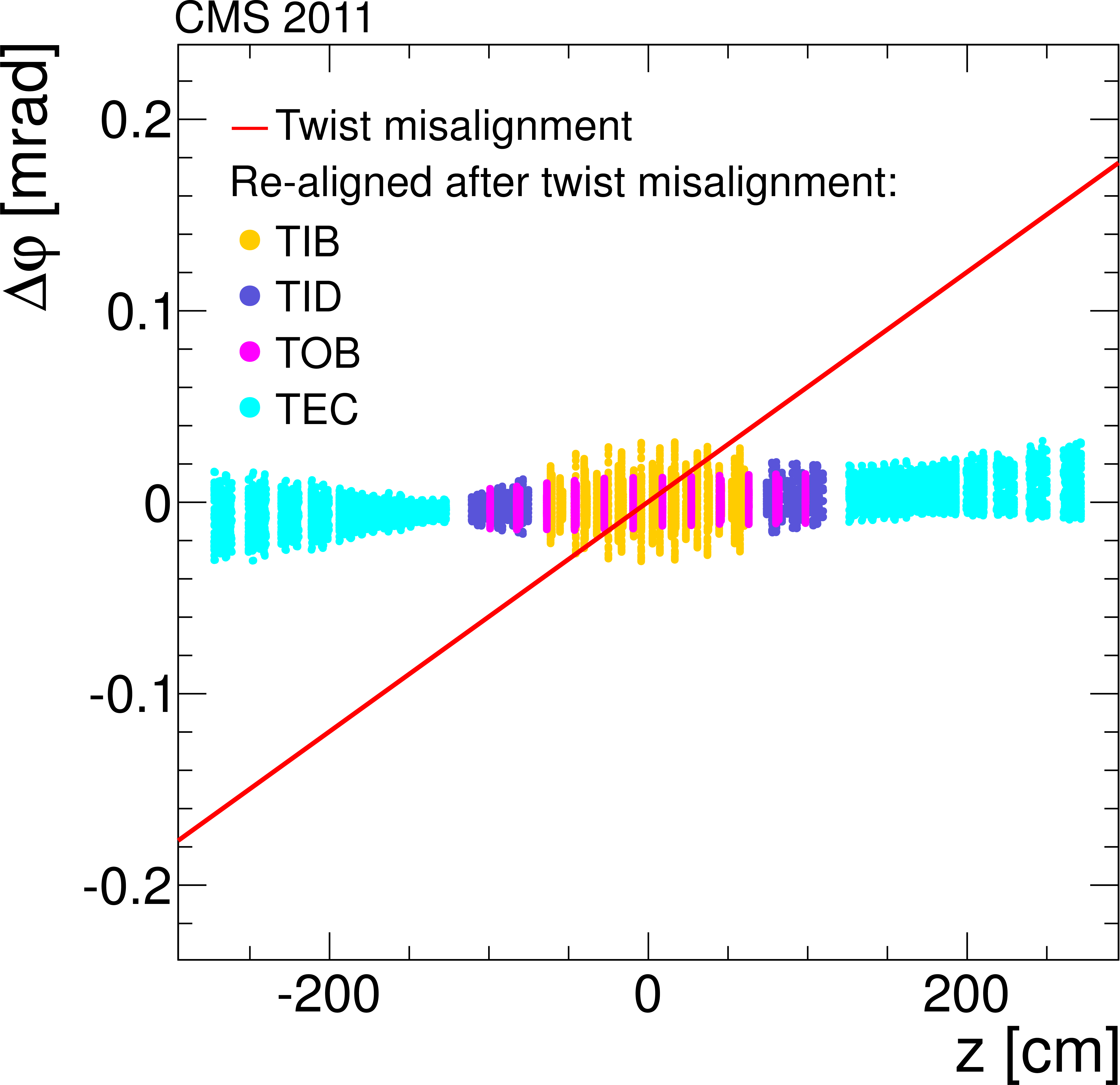
Figure 19-a:
Impact of intentional application of a twist (a, b), sagitta (c, d) and skew systematic misalignment (e, f). In the (a, c, e) plots, the red line shows the size of the applied misalignment, and the coloured dots show the difference of selected alignment parameters, module by module after realignment, to the initial values prior to misalignment. The (b, d, f) plots show the distributions of goodness-of-fit for loosely selected isolated muons from an independent data sample, with transverse momentum $ {p_{\mathrm {T}}} > $ 5 GeV/$c$. |
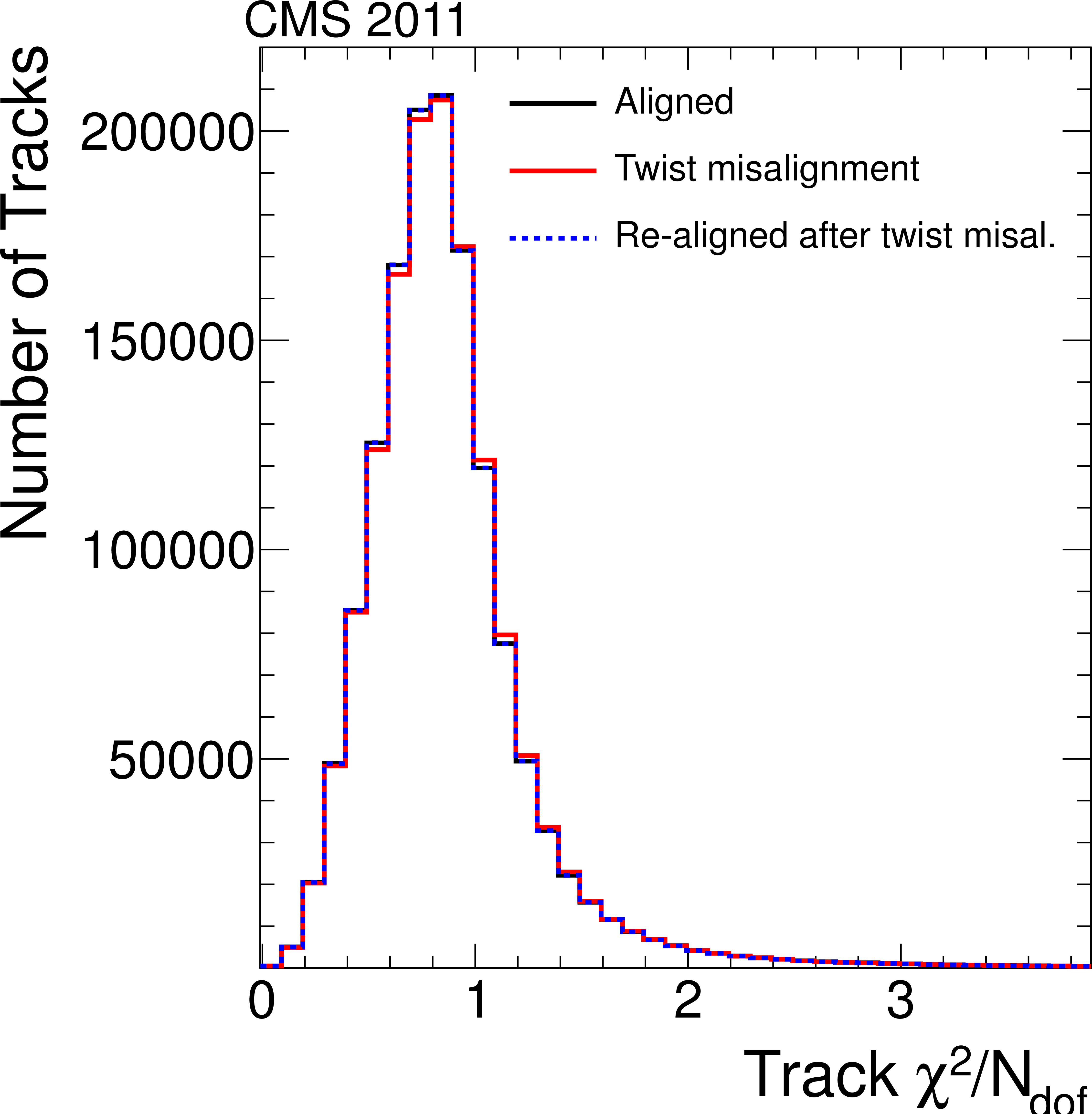
png pdf |
Figure 19-b:
Impact of intentional application of a twist (a, b), sagitta (c, d) and skew systematic misalignment (e, f). In the (a, c, e) plots, the red line shows the size of the applied misalignment, and the coloured dots show the difference of selected alignment parameters, module by module after realignment, to the initial values prior to misalignment. The (b, d, f) plots show the distributions of goodness-of-fit for loosely selected isolated muons from an independent data sample, with transverse momentum $ {p_{\mathrm {T}}} > $ 5 GeV/$c$. |
png pdf |
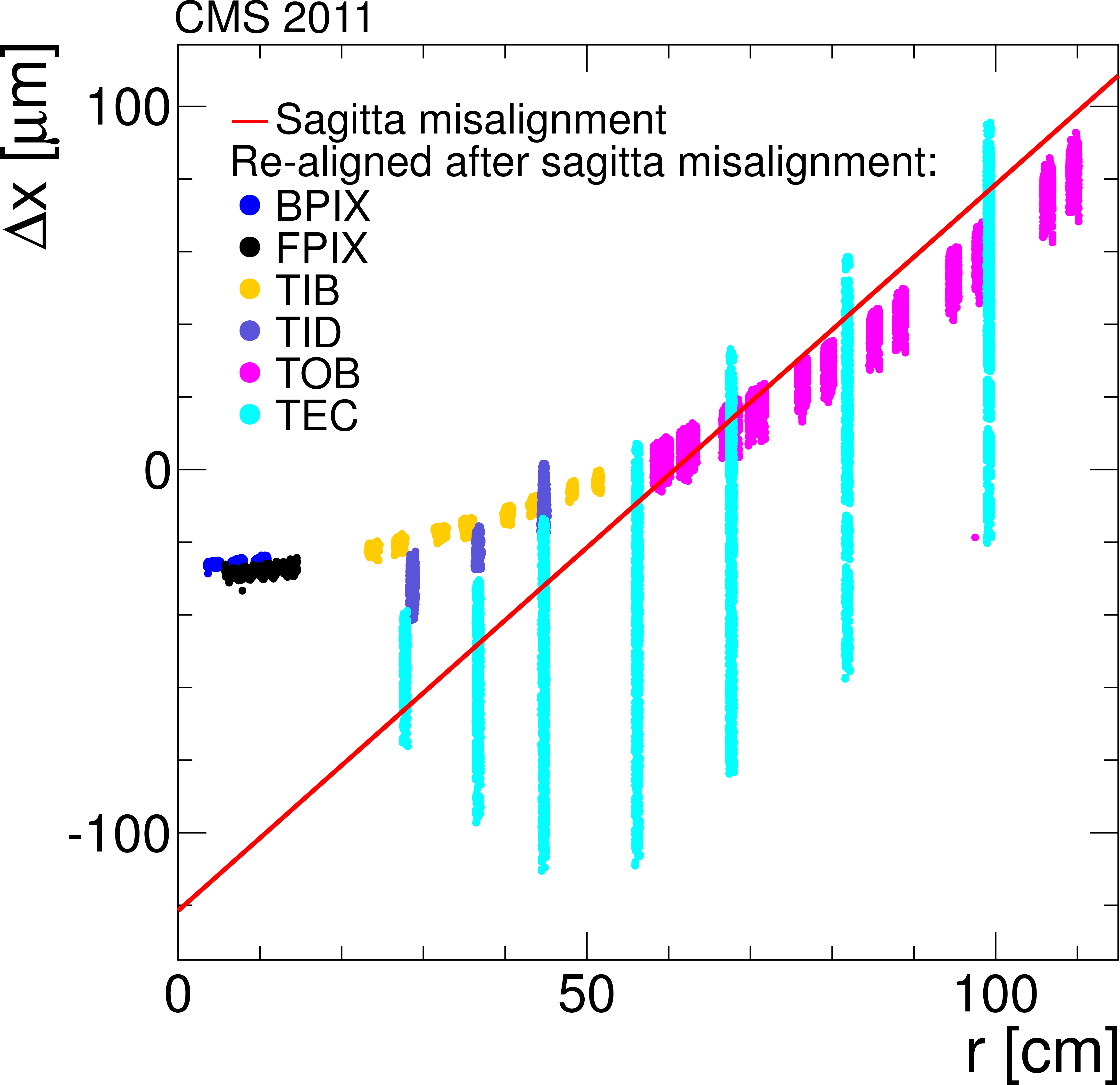
Figure 19-c:
Impact of intentional application of a twist (a, b), sagitta (c, d) and skew systematic misalignment (e, f). In the (a, c, e) plots, the red line shows the size of the applied misalignment, and the coloured dots show the difference of selected alignment parameters, module by module after realignment, to the initial values prior to misalignment. The (b, d, f) plots show the distributions of goodness-of-fit for loosely selected isolated muons from an independent data sample, with transverse momentum $ {p_{\mathrm {T}}} > $ 5 GeV/$c$. |

png pdf |
Figure 19-d:
Impact of intentional application of a twist (a, b), sagitta (c, d) and skew systematic misalignment (e, f). In the (a, c, e) plots, the red line shows the size of the applied misalignment, and the coloured dots show the difference of selected alignment parameters, module by module after realignment, to the initial values prior to misalignment. The (b, d, f) plots show the distributions of goodness-of-fit for loosely selected isolated muons from an independent data sample, with transverse momentum $ {p_{\mathrm {T}}} > $ 5 GeV/$c$. |

png pdf |
Figure 19-e:
Impact of intentional application of a twist (a, b), sagitta (c, d) and skew systematic misalignment (e, f). In the (a, c, e) plots, the red line shows the size of the applied misalignment, and the coloured dots show the difference of selected alignment parameters, module by module after realignment, to the initial values prior to misalignment. The (b, d, f) plots show the distributions of goodness-of-fit for loosely selected isolated muons from an independent data sample, with transverse momentum $ {p_{\mathrm {T}}} > $ 5 GeV/$c$. |

png pdf |
Figure 19-f:
Impact of intentional application of a twist (a, b), sagitta (c, d) and skew systematic misalignment (e, f). In the (a, c, e) plots, the red line shows the size of the applied misalignment, and the coloured dots show the difference of selected alignment parameters, module by module after realignment, to the initial values prior to misalignment. The (b, d, f) plots show the distributions of goodness-of-fit for loosely selected isolated muons from an independent data sample, with transverse momentum $ {p_{\mathrm {T}}} > $ 5 GeV/$c$. |
|
|
Compact Muon Solenoid LHC, CERN |
|

|

|

|

|

|