Design and performance of the LHCb trigger and full real-time reconstruction in Run 2 of the LHC
[to restricted-access page]Information
LHCb-DP-2019-001
arXiv:1812.10790 [PDF]
(Submitted on 27 Dec 2018)
JINST 14 (2019) P04013
Inspire 1711636
Tools
Abstract
The LHCb collaboration has redesigned its trigger to enable the full offline detector reconstruction to be performed in real time. Together with the real-time alignment and calibration of the detector, and a software infrastructure to make persistent the high-level physics objects produced during real-time processing, this redesign enabled the widespread deployment of real-time analysis during Run 2. We describe the design of the Run 2 trigger and real-time reconstruction, and present data-driven performance measurements for a representative sample of LHCb's physics programme.
Figures and captions
|
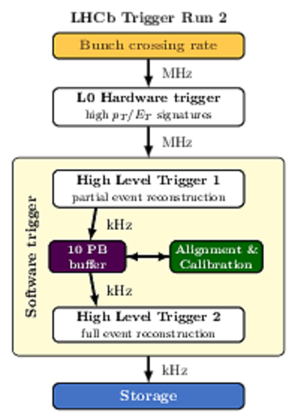
Overview of the LHCb trigger system. |
Fig_1.pdf [69 KiB] HiDef png [657 KiB] Thumbnail [541 KiB] tex code |
|
|
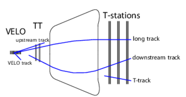
Sketch of the different types of tracks within LHCb . |
lhcb_t[..].pdf [247 KiB] HiDef png [108 KiB] Thumbnail [69 KiB] |
|
|
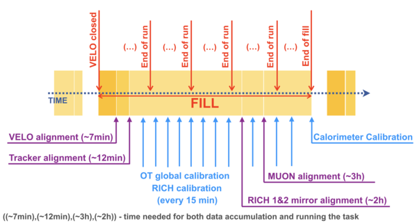
Schematic view of the real-time alignment and calibration procedure starting at the beginning of each fill, as used for 2018 data taking. |
alignm[..].png [358 KiB] HiDef png [117 KiB] Thumbnail [61 KiB] |
|
|
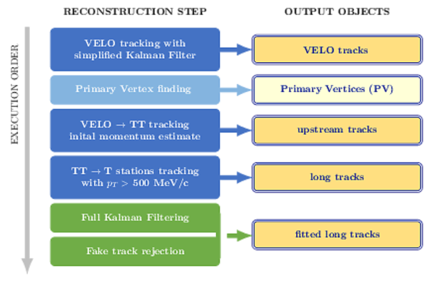
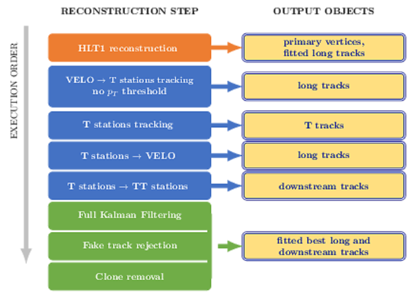
Sketch of the HLT1 track and vertex reconstruction. |
Fig_4.pdf [53 KiB] HiDef png [396 KiB] Thumbnail [235 KiB] tex code |
|
|
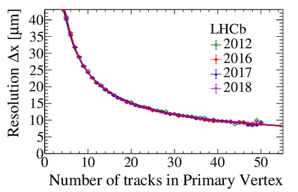
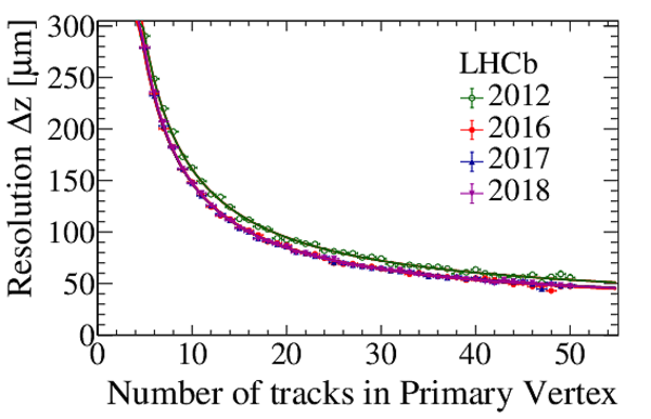
The PV $x$ (left) and $z$ (right) resolution as a function of the number of tracks in the PV for the Run 1 off\-line and Run 2 (used both off\-line and online) PV reconstruction algorithms. |
resolu[..].pdf [30 KiB] HiDef png [251 KiB] Thumbnail [181 KiB] |
|
|
resolu[..].pdf [29 KiB] HiDef png [299 KiB] Thumbnail [198 KiB] |
|
|
|
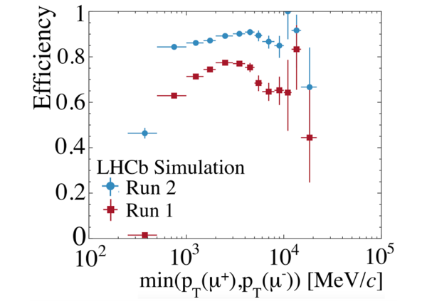
HLT1 dimuon efficiency as a function of the minimum $p_{\rm T}$ of the two muons. A large gain, especially at low $p_{\rm T}$ , can be seen from the comparison of the Run 1 and Run 2 algorithms. |
hlt1_d[..].pdf [286 KiB] HiDef png [221 KiB] Thumbnail [140 KiB] |
|
|
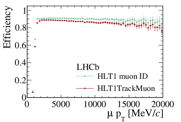
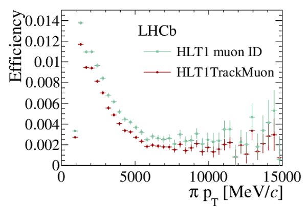
HLT1 muon identification efficiency for (left) muons from $ { J \mskip -3mu/\mskip -2mu\psi \mskip 2mu} \rightarrow \mu ^+\mu ^- $ decays and (right) pions from $ D^0 \rightarrow K ^- \pi ^+ $ decays. Green circles show only the identification efficiency (HLT1 Muon ID) while red squares show the efficiency of the additional trigger line (named HLT1TrackMuon) requirements (see text). |
Hlt1Tr[..].pdf [19 KiB] HiDef png [214 KiB] Thumbnail [168 KiB] |
|
|
Hlt1Tr[..].pdf [18 KiB] HiDef png [219 KiB] Thumbnail [185 KiB] |
|
|
|
Sketch of the HLT2 track and vertex reconstruction sequence. |
Fig_8.pdf [69 KiB] HiDef png [428 KiB] Thumbnail [251 KiB] tex code |
|
|
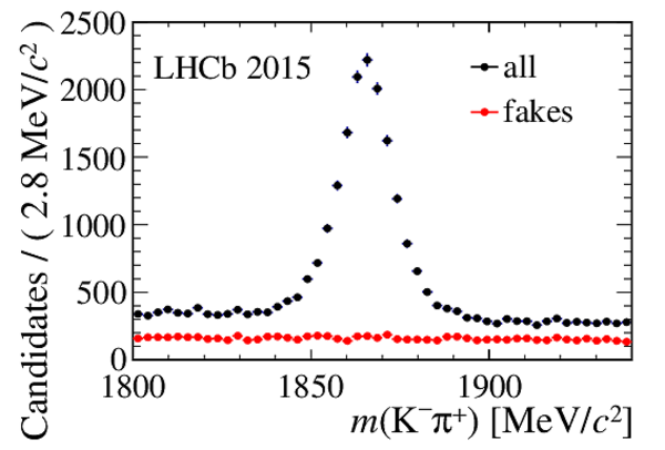
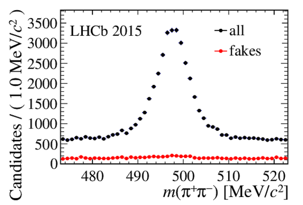
Performance of the fake-track classifier on (left) $ D \rightarrow K ^- \pi ^+ $ and (right) $ K ^0_{\rm\scriptscriptstyle S} \rightarrow \pi ^- \pi ^+ $ decays. For these plots, the clones have been removed. |
DGhostProb.pdf [18 KiB] HiDef png [196 KiB] Thumbnail [172 KiB] |
|
|
KsGhos[..].pdf [18 KiB] HiDef png [213 KiB] Thumbnail [200 KiB] |
|
|
|
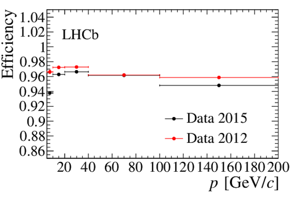
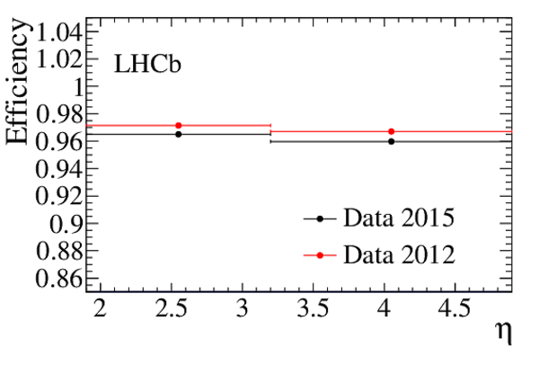
Comparison of the track reconstruction efficiency in 2015 and 2012 data as a function of the momentum (left) and pseudorapidity (right). |
P_Comp[..].pdf [14 KiB] HiDef png [164 KiB] Thumbnail [171 KiB] |
|
|
Eta_Co[..].pdf [14 KiB] HiDef png [127 KiB] Thumbnail [133 KiB] |
|
|
|
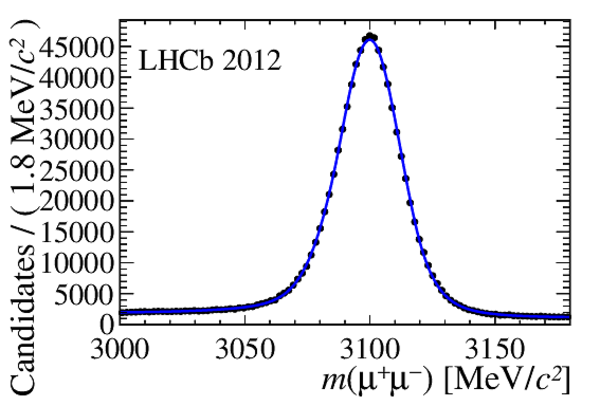
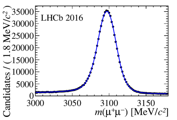
Comparison of the invariant mass distributions for a subset of the 2012 (left) and 2016 (right) data set, using $ { J \mskip -3mu/\mskip -2mu\psi \mskip 2mu} \rightarrow \mu ^+\mu ^- $ decays, with the $ { J \mskip -3mu/\mskip -2mu\psi \mskip 2mu}$ originating from a $ b $ -hadron. |
Jpsi2012.pdf [25 KiB] HiDef png [224 KiB] Thumbnail [211 KiB] |
|
|
Jpsi2016.pdf [24 KiB] HiDef png [209 KiB] Thumbnail [193 KiB] |
|
|
|
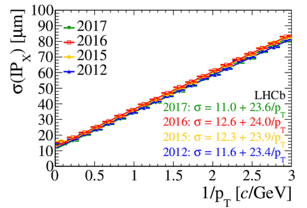
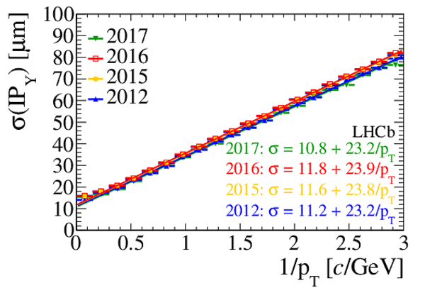
Resolution of the $x$ (left) and $y$ (right) components of the impact parameter comparing the 2012 (blue), 2015 (orange), 2016 (red) and 2017 (green) data-taking periods. The resolution as a function of $p_{\rm T}$ is given in the bottom right corner. |
IPX.pdf [20 KiB] HiDef png [308 KiB] Thumbnail [225 KiB] |
|
|
IPY.pdf [20 KiB] HiDef png [308 KiB] Thumbnail [227 KiB] |
|
|
|
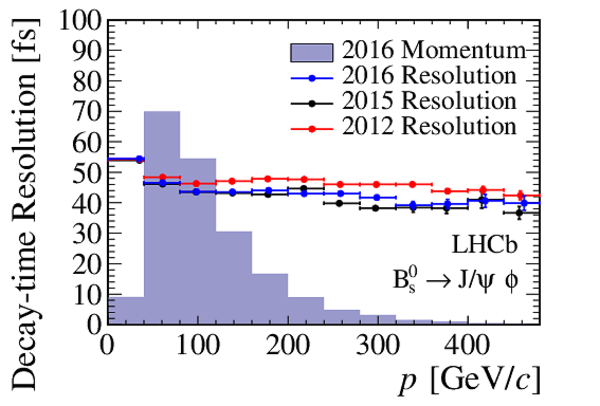
Decay time resolution for $ B ^0_ s \rightarrow { J \mskip -3mu/\mskip -2mu\psi \mskip 2mu} \phi$ decays (in their rest frame) as a function of momentum. The filled histogram shows the distribution of $ B ^0_ s $ meson momenta, to give an idea of the relative importance of the different resolution bins for the analysis sensitivity. |
final_[..].pdf [16 KiB] HiDef png [225 KiB] Thumbnail [225 KiB] |
|
|
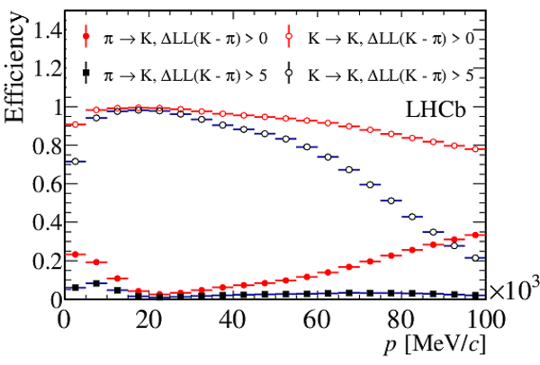
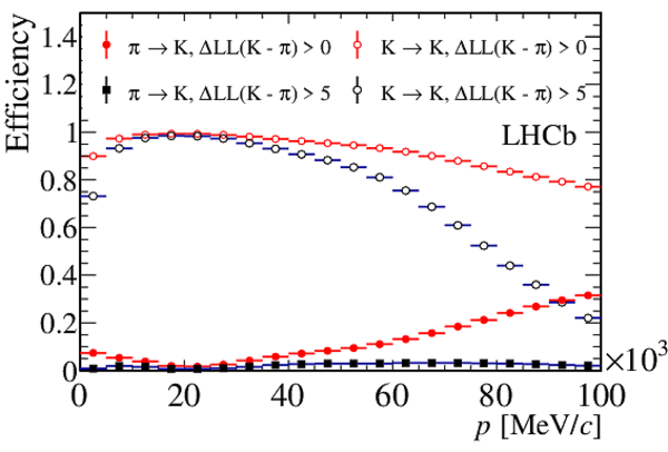
Efficiency and fake rate of the RICH identification for the 2012 (left) and the 2016 (right) data. |
RICHPe[..].pdf [17 KiB] HiDef png [199 KiB] Thumbnail [182 KiB] |
|
|
RICHPe[..].pdf [17 KiB] HiDef png [197 KiB] Thumbnail [180 KiB] |
|
|
|
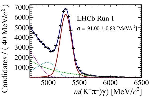
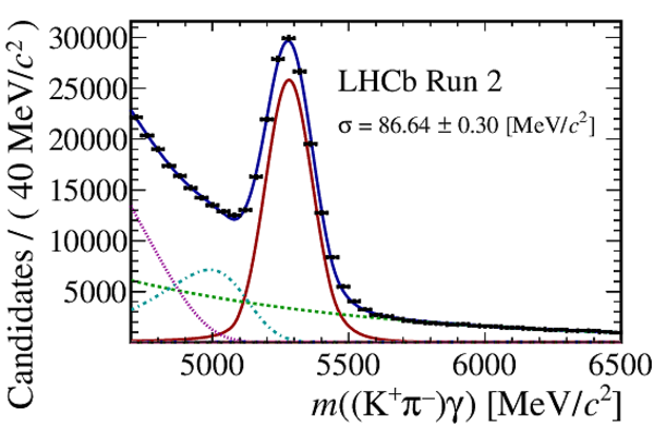
Invariant mass of $B^0 \rightarrow (K^+ \pi^-) \gamma$ candidates in Run 1 (left) and Run 2 (right). The fit model includes the (red) signal component, (dashed green) combinatorial background, (dot-dashed turqoise) misidentified physics backgrounds (e.g. $ B ^0_ s \rightarrow \phi\gamma$ where a kaon is misidentified as a pion) and (dotted magenta) partially reconstructed physics backgrounds. |
kpiG_run1.pdf [22 KiB] HiDef png [328 KiB] Thumbnail [242 KiB] |
|
|
kpiG_run2.pdf [22 KiB] HiDef png [332 KiB] Thumbnail [246 KiB] |
|
|
|
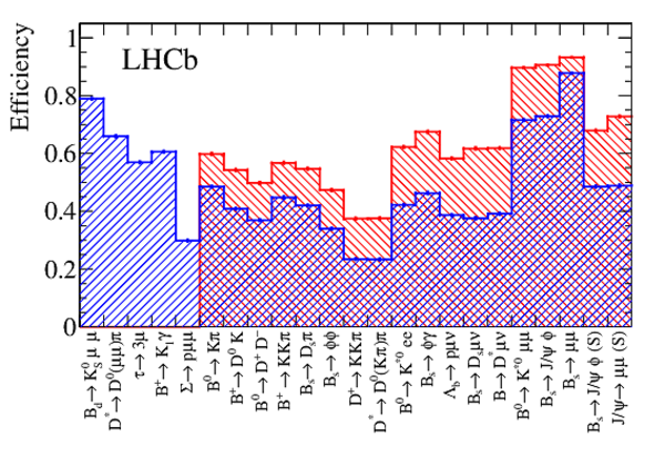
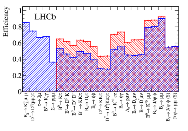
Efficiencies per signal mode for (top) 2016 and (bottom) 2017 data-taking periods measured in simulation. Red (left-slanted) hatched plots are when the entire \texttt{L0} bandwidth is granted to this signal mode, whereas blue (right-slanted) hatched plots are following the bandwidth division. Signals which appear only in blue are used for performance validation and are not part of the optimization itself. Channels followed by "(S)" are selected in a kinematic and geometric volume which is particularly important for spectroscopy studies. |
2220b_[..].pdf [20 KiB] HiDef png [1 MiB] Thumbnail [512 KiB] |
|
|
1868b_[..].pdf [20 KiB] HiDef png [1 MiB] Thumbnail [536 KiB] |
|
|
|
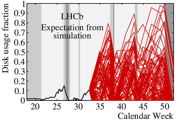
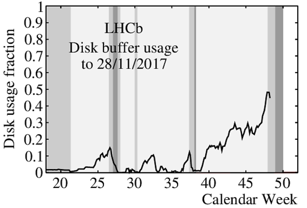
Disk buffer usage projections during (left) and at the end of (right) the 2017 data-taking period. During data taking, simulations (red, left) are used every two weeks to determine the probability of exceeding the 80% usage threshold. In 2017, the loose HLT1 configuration was used for the entire year leading to a maximum buffer capacity of 48% (black, right). LHC Technical Stops and Machine Development (MD) periods are shown in dark and light grey, respectively. The schedule changed between when this simulation was run in week 32 and the end of the year. An MD period was removed and the duration of the data taking was reduced. |
Simulation.pdf [69 KiB] HiDef png [993 KiB] Thumbnail [479 KiB] |
|
|
Usage2[..].pdf [15 KiB] HiDef png [205 KiB] Thumbnail [190 KiB] |
|
|
|
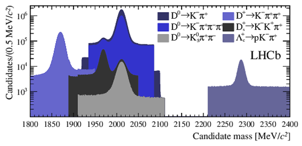
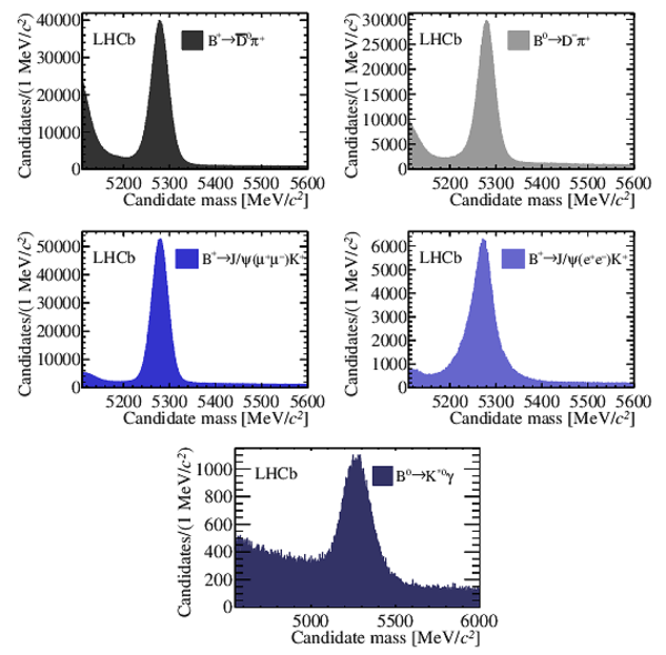
Charm candidates used for the evaluation of the trigger performance. |
CharmS[..].pdf [100 KiB] HiDef png [228 KiB] Thumbnail [194 KiB] |
|
|
Beauty candidates used for the evaluation of the trigger performance. |
Beauty[..].pdf [56 KiB] HiDef png [473 KiB] Thumbnail [414 KiB] |
|
|
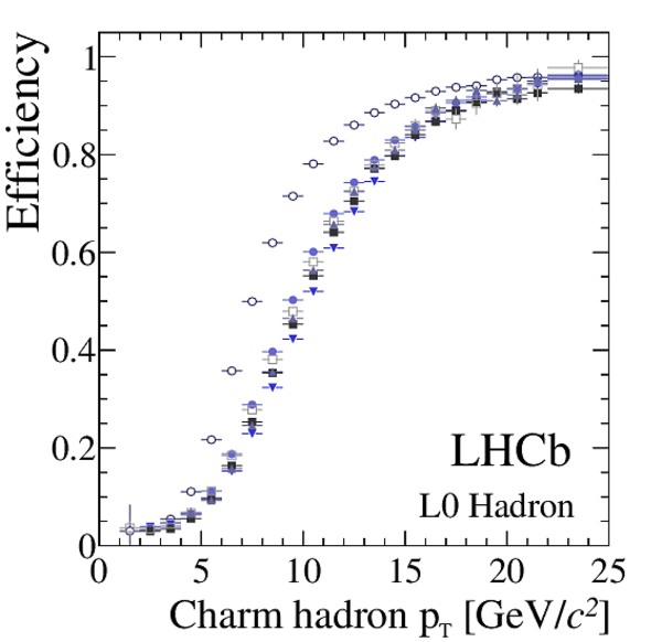
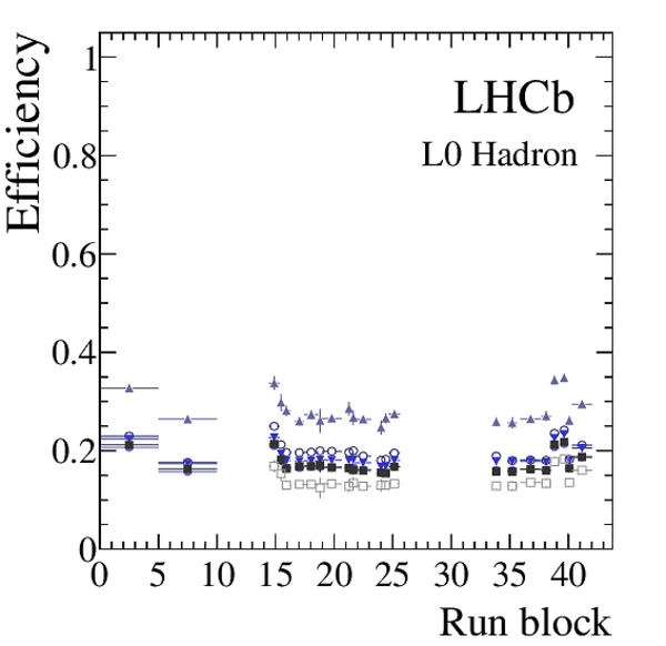
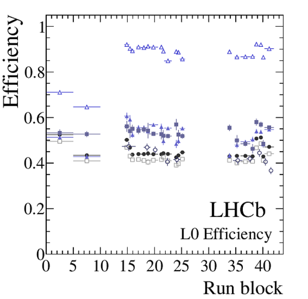
Efficiencies of the \texttt{L0} trigger lines in Run 2 data for $ c$ -hadron decays. The left plot shows the efficiency as a function of the hadron $p_{\rm T}$ , while the right plot shows the evolution of the efficiency as a function of the different trigger configurations used during data taking. The three blocks visible in the plot, separated by vertical gaps, correspond to the three years of data taking (2015--2017). The \texttt{L0} hadron efficiency is shown. |
L0_Cha[..].pdf [12 KiB] HiDef png [42 KiB] Thumbnail [37 KiB] |

|
|
L0HadE[..].pdf [18 KiB] HiDef png [234 KiB] Thumbnail [190 KiB] |
|
|
|
L0HadE[..].pdf [18 KiB] HiDef png [218 KiB] Thumbnail [180 KiB] |
|
|
|
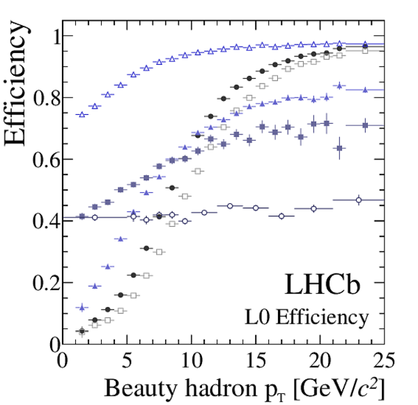
Efficiencies of the \texttt{L0} trigger lines in Run 2 data for $ b$ -hadron decays. The left plot shows the efficiency as a function of the hadron $p_{\rm T}$ , while the right plot shows the evolution of the efficiency as a function of the different trigger configurations used during data taking. The three blocks visible in the plot, separated by vertical gaps, correspond to the three years of data taking (2015--2017). The plotted \texttt{L0} efficiency for each $ b$ -hadron is described in the legend above the plots. |
L0_Bea[..].pdf [13 KiB] HiDef png [58 KiB] Thumbnail [49 KiB] |

|
|
L0Eff_[..].pdf [19 KiB] HiDef png [259 KiB] Thumbnail [226 KiB] |
|
|
|
L0Eff_[..].pdf [18 KiB] HiDef png [240 KiB] Thumbnail [198 KiB] |
|
|
|
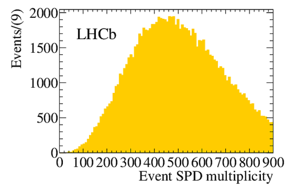
The SPD hit multiplicity of events containing $ B ^+ \rightarrow \overline{ D }{} {}^0 \pi ^+ $ candidates in Run 2 data. |
nSPD.pdf [14 KiB] HiDef png [152 KiB] Thumbnail [140 KiB] |
|
|
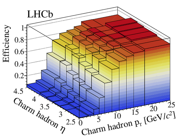
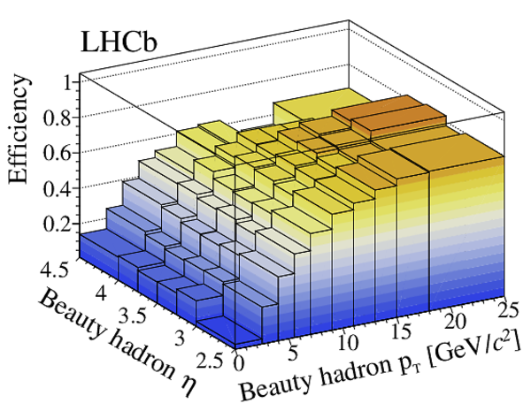
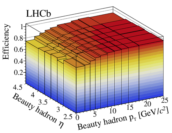
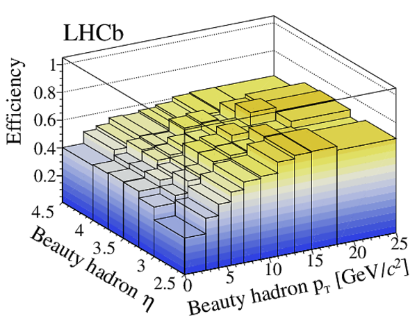
Two-dimensional efficiencies of the \texttt{L0} trigger lines in Run 2 data: (top left) \texttt{L0} hadron; (top right) \texttt{L0} electron; (bottom left) \texttt{L0} muon; and (bottom right) \texttt{L0} dimuon. The \texttt{L0} hadron efficiency is evaluated using $ D ^0 \rightarrow K ^- \pi ^+ $ decays, whereas the others are evaluated using the relevant signals listed in Fig. 20 and Fig. 21. |
L0HadE[..].pdf [63 KiB] HiDef png [1 MiB] Thumbnail [621 KiB] |
|
|
L0EleE[..].pdf [59 KiB] HiDef png [1 MiB] Thumbnail [578 KiB] |
|
|
|
L0MuEf[..].pdf [86 KiB] HiDef png [1 MiB] Thumbnail [613 KiB] |
|
|
|
L0DiMu[..].pdf [61 KiB] HiDef png [1 MiB] Thumbnail [571 KiB] |
|
|
|
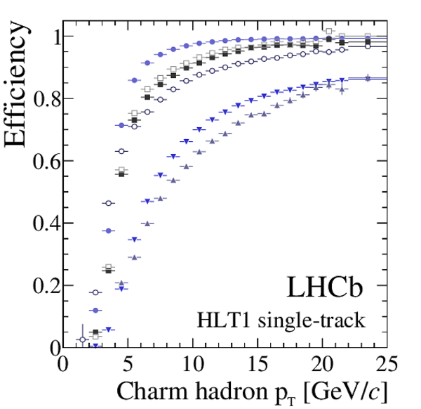
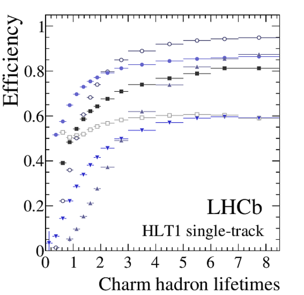
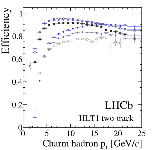
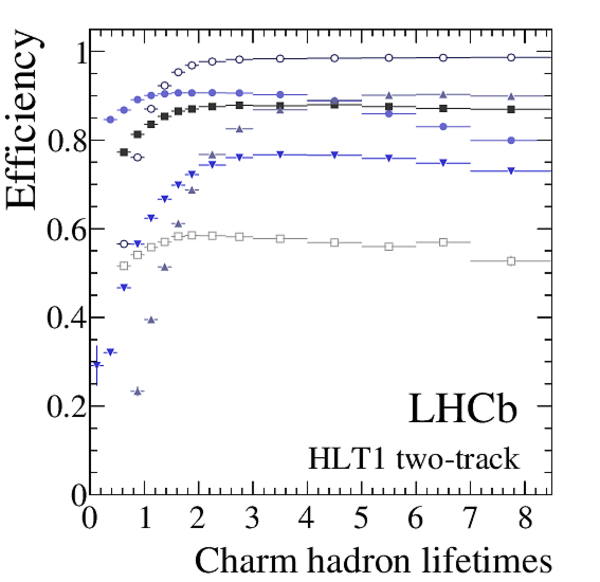
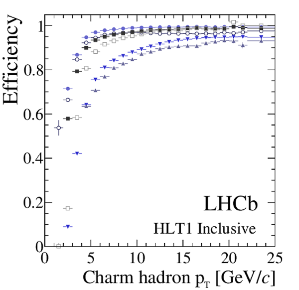
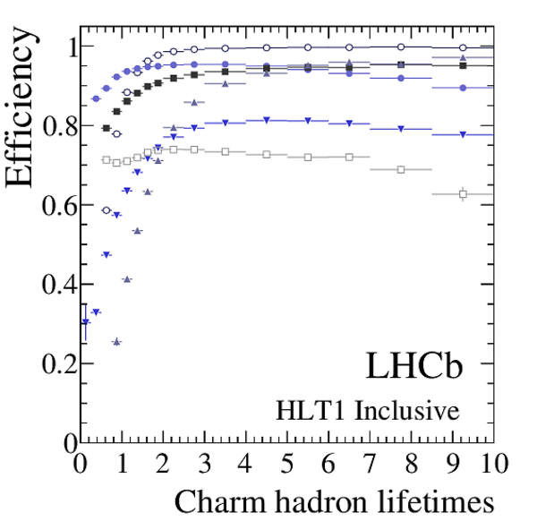
Efficiency of the HLT1 inclusive trigger lines as a function of (left) $ c$ -hadron $p_{\rm T}$ and (right) decay time. The decay time plots are drawn such that the x-axis is binned in units of the lifetime for each hadron in its rest frame. The plots in each column show, from top to bottom, the single-track, two-track, and combined HLT1 inclusive performance. |
L0_Cha[..].pdf [12 KiB] HiDef png [42 KiB] Thumbnail [37 KiB] |
|
|
HLT1Tr[..].pdf [18 KiB] HiDef png [253 KiB] Thumbnail [216 KiB] |
|
|
|
HLT1Tr[..].pdf [17 KiB] HiDef png [214 KiB] Thumbnail [190 KiB] |
|
|
|
HLT1Tw[..].pdf [18 KiB] HiDef png [239 KiB] Thumbnail [208 KiB] |
|
|
|
HLT1Tw[..].pdf [16 KiB] HiDef png [210 KiB] Thumbnail [187 KiB] |
|
|
|
HLT1To[..].pdf [18 KiB] HiDef png [237 KiB] Thumbnail [201 KiB] |
|
|
|
HLT1To[..].pdf [17 KiB] HiDef png [218 KiB] Thumbnail [193 KiB] |
|
|
|
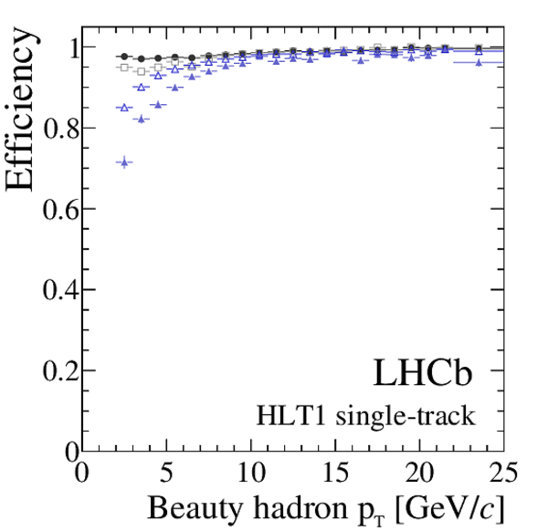
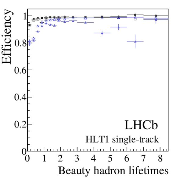
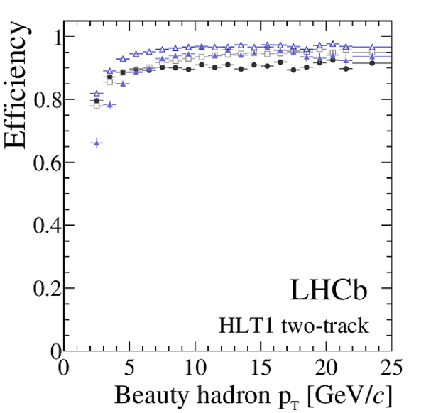
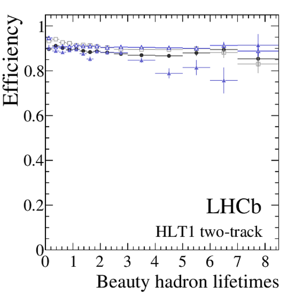
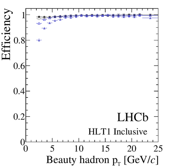
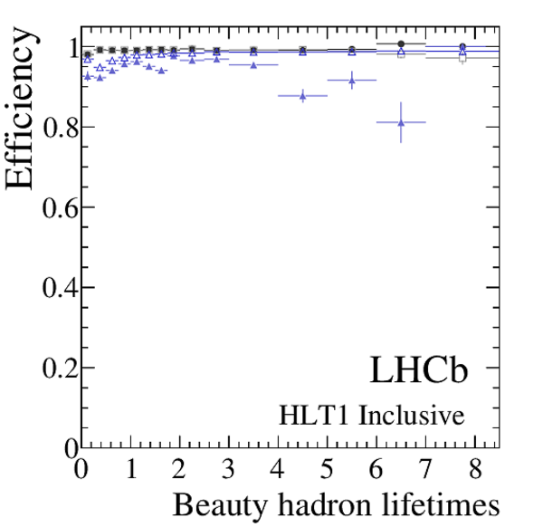
Efficiency of the HLT1 inclusive trigger lines as a function of (left) $ b$ -hadron $p_{\rm T}$ and (right) decay time. The decay time plots are drawn such that the x-axis is binned in units of the lifetime for each hadron in its rest frame. The plots in each column show, from top to bottom, the single-track, two-track, and combined HLT1 inclusive performance. |
HLT1_B[..].pdf [12 KiB] HiDef png [33 KiB] Thumbnail [30 KiB] |

|
|
HLT1Tr[..].pdf [16 KiB] HiDef png [200 KiB] Thumbnail [168 KiB] |
|
|
|
HLT1Tr[..].pdf [15 KiB] HiDef png [179 KiB] Thumbnail [148 KiB] |
|
|
|
HLT1Tw[..].pdf [17 KiB] HiDef png [206 KiB] Thumbnail [179 KiB] |
|
|
|
HLT1Tw[..].pdf [16 KiB] HiDef png [188 KiB] Thumbnail [164 KiB] |
|
|
|
HLT1To[..].pdf [16 KiB] HiDef png [188 KiB] Thumbnail [156 KiB] |
|
|
|
HLT1To[..].pdf [16 KiB] HiDef png [180 KiB] Thumbnail [158 KiB] |
|
|
|
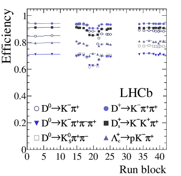
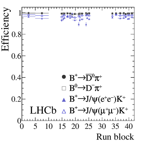
The HLT1 efficiency as a function of the different trigger configurations used during data taking for (left) $ c$ -hadrons and (right) $ b$ -hadrons. The three blocks visible in the plot, separated by vertical gaps, correspond to the three years of data taking (2015--2017). |
HLT1To[..].pdf [18 KiB] HiDef png [281 KiB] Thumbnail [244 KiB] |
|
|
HLT1To[..].pdf [17 KiB] HiDef png [229 KiB] Thumbnail [201 KiB] |
|
|
|
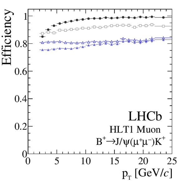
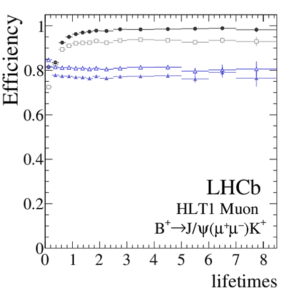
The efficiency of the HLT1 muon trigger lines as a function of the (left) $ b$ -hadron $p_{\rm T}$ and (right) units of the average $ B ^+ $ decay time. The decay time plot is drawn such that the x-axis is binned in units of the $ B ^+ $ lifetime in its rest frame. The efficiency of the inclusive single-track HLT1 trigger is plotted for reference. |
HLT1Mu[..].pdf [12 KiB] HiDef png [32 KiB] Thumbnail [26 KiB] |

|
|
HLT1Mu[..].pdf [17 KiB] HiDef png [201 KiB] Thumbnail [181 KiB] |
|
|
|
HLT1Mu[..].pdf [16 KiB] HiDef png [183 KiB] Thumbnail [169 KiB] |
|
|
|
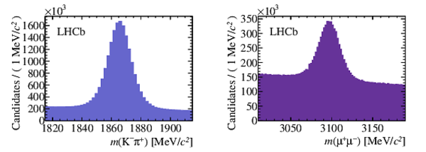
The $D^0$ (left) and $J/\psi$ (right) candidates selected by the HLT1 calibration lines. Both plots show candidates reconstructed online. |
online[..].pdf [16 KiB] HiDef png [170 KiB] Thumbnail [150 KiB] |
|
|
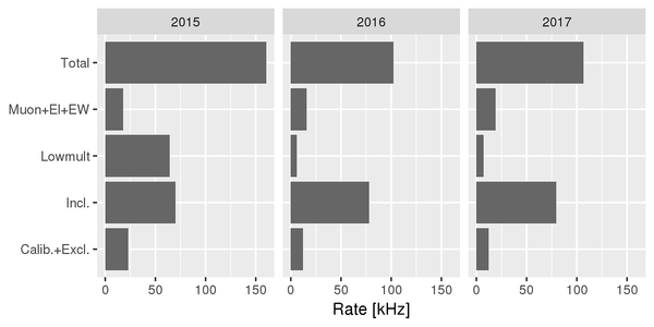
Rates of the main groups of HLT1 trigger lines and the total HLT1 rate as a function of the year of data taking, shown for the trigger configuration used to take most of the luminosity in each year. |
hlt1_rates.png [25 KiB] HiDef png [18 KiB] Thumbnail [11 KiB] |
|
|
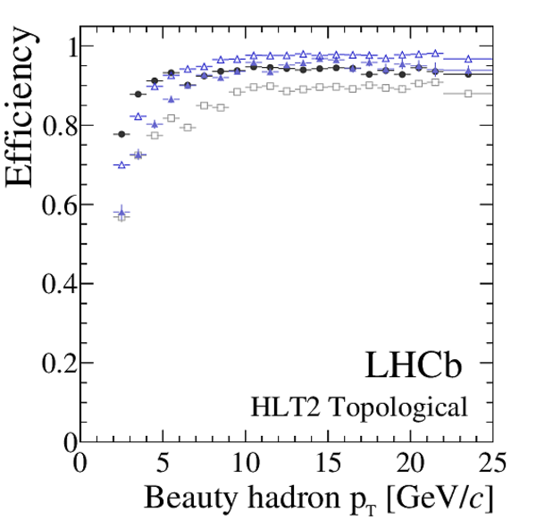
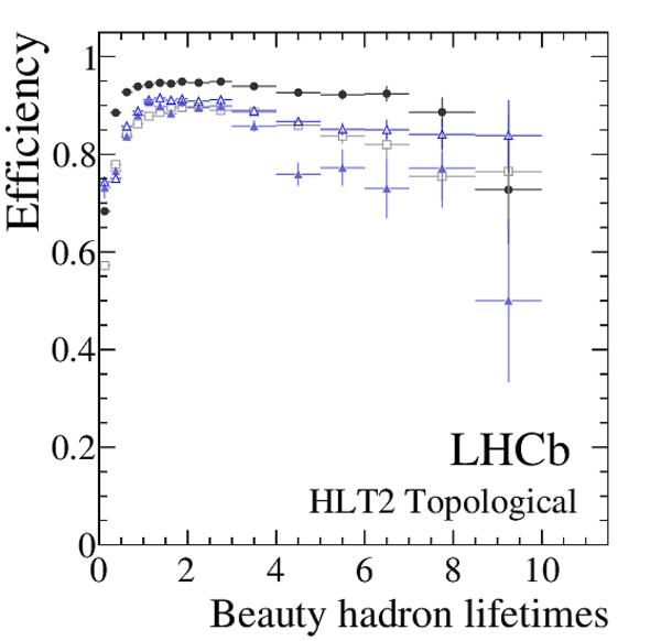
Efficiency of the HLT2 topological trigger lines as a function of the (left) $ b$ -hadron $p_{\rm T}$ and (right) in units of the average $ b$ -hadron decay time. The decay time plots are drawn such that the x-axis is binned in units of the lifetime for each hadron in its rest frame. The plots show the combined efficiency of the topological trigger lines for each $ b$ -hadron decay mode. |
HLT2To[..].pdf [12 KiB] HiDef png [34 KiB] Thumbnail [31 KiB] |

|
|
HLT2To[..].pdf [17 KiB] HiDef png [211 KiB] Thumbnail [186 KiB] |
|
|
|
HLT2To[..].pdf [16 KiB] HiDef png [193 KiB] Thumbnail [165 KiB] |
|
|
|
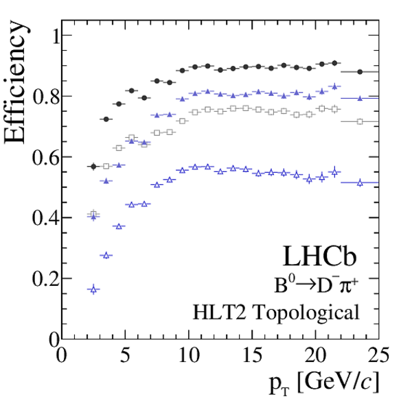
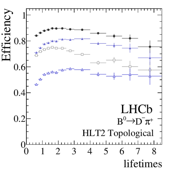
Efficiency of the HLT2 topological trigger lines as a function of the (left) $ b$ -hadron $p_{\rm T}$ and (right) in units of the average $ b$ -hadron decay time. The decay time plots are drawn such that the x-axis is binned in units of the lifetime for each hadron in its rest frame. The plots show the different contributions of the 2-, 3-, and 4-body topological trigger lines to a specific decay. |
HLT2To[..].pdf [12 KiB] HiDef png [38 KiB] Thumbnail [30 KiB] |

|
|
HLT2To[..].pdf [17 KiB] HiDef png [210 KiB] Thumbnail [187 KiB] |
|
|
|
HLT2To[..].pdf [16 KiB] HiDef png [181 KiB] Thumbnail [168 KiB] |
|
|
|
Evolution of the HLT2 efficiency as a function of the different trigger configurations used during data taking. |
HLT2To[..].pdf [17 KiB] HiDef png [237 KiB] Thumbnail [211 KiB] |
|
|
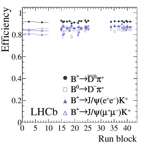
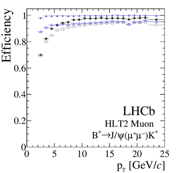
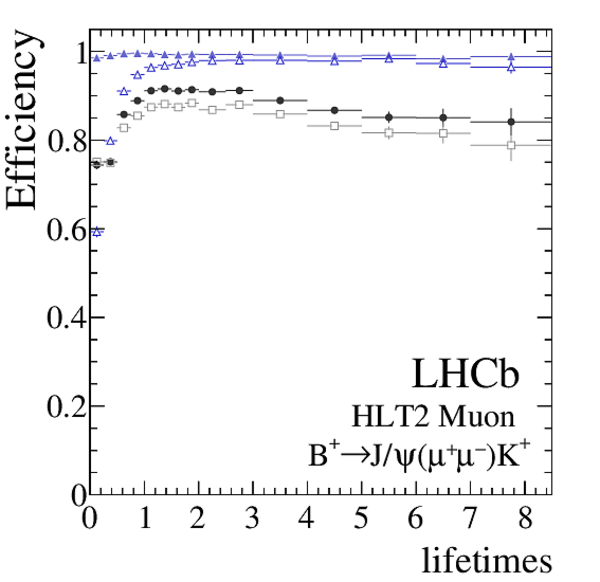
The TOS efficiency of the HLT2 muon trigger lines as a function of the (left) $ B ^+ $ $p_{\rm T}$ and (right) units of the average $ B ^+ $ decay time. The decay time plot is drawn such that the x-axis is binned in units of the $ B ^+ $ lifetime in its rest frame. The efficiency of the inclusive topological ("any topological") trigger lines and topological trigger lines requiring one track identified as a muon ("any muon topological") are plotted for reference. |
HLT2Mu[..].pdf [12 KiB] HiDef png [36 KiB] Thumbnail [29 KiB] |

|
|
HLT2Mu[..].pdf [16 KiB] HiDef png [198 KiB] Thumbnail [176 KiB] |
|
|
|
HLT2Mu[..].pdf [16 KiB] HiDef png [181 KiB] Thumbnail [168 KiB] |
|
|
|
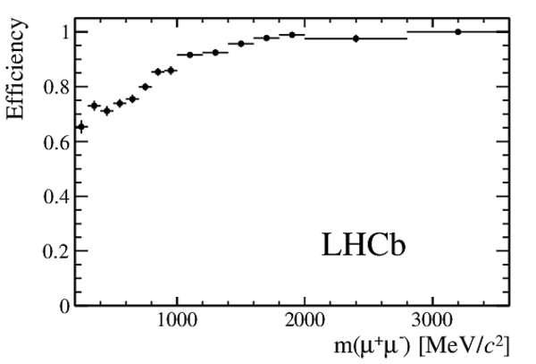
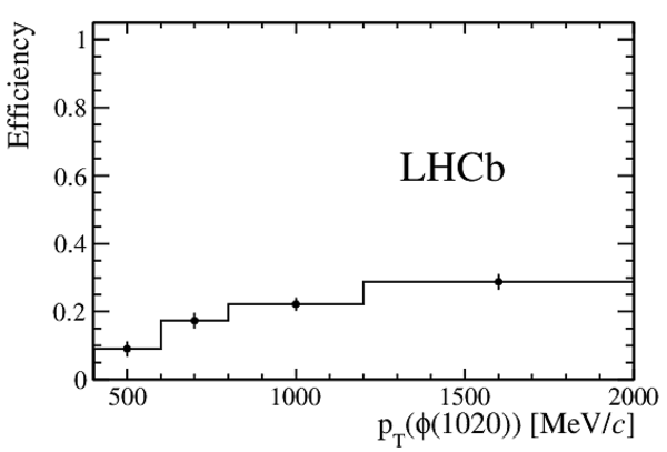
HLT2 trigger efficiencies of the dedicated selections for low-multiplicity events: (left) for dimuon candidates as a function of dimuon mass, and (right) for $\phi(1020)$ candidates as a function of candidate $p_{\rm T}$ . |
eff_Hl[..].pdf [14 KiB] HiDef png [68 KiB] Thumbnail [41 KiB] |
|
|
eff_Hl[..].pdf [13 KiB] HiDef png [69 KiB] Thumbnail [40 KiB] |
|
|
|
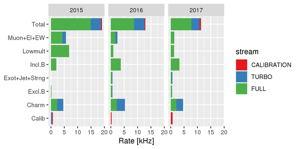
Rates of the main categories of HLT2 trigger lines and the total HLT2 rate for each year of data taking, shown for the trigger configuration used to take most of the luminosity in the given year. TURBO, CALIBRATION, and FULL refer to different output data streams as discussed in Ref. [2]. |
hlt2_rates.png [54 KiB] HiDef png [64 KiB] Thumbnail [39 KiB] |
|
|
Animated gif made out of all figures. |
DP-2019-001.gif Thumbnail |

|
![HiDef png [657 KiB]](Directory_LHCb-DP-2019-001/hidef_Fig_1.png)
![HiDef png [108 KiB]](Directory_LHCb-DP-2019-001/hidef_lhcb_tracks.png)
![alignm[..].png [358 KiB]](Directory_LHCb-DP-2019-001/alignmentAndCalibration.png)
![HiDef png [117 KiB]](Directory_LHCb-DP-2019-001/hidef_alignmentAndCalibration.png)
![HiDef png [396 KiB]](Directory_LHCb-DP-2019-001/hidef_Fig_4.png)
![HiDef png [251 KiB]](Directory_LHCb-DP-2019-001/hidef_resolution_run1_vs_201620172018_x.png)
![HiDef png [299 KiB]](Directory_LHCb-DP-2019-001/hidef_resolution_run1_vs_201620172018_z.png)
![HiDef png [221 KiB]](Directory_LHCb-DP-2019-001/hidef_hlt1_dimuon_eff_new.png)
![HiDef png [214 KiB]](Directory_LHCb-DP-2019-001/hidef_Hlt1TrackMuon_eff.png)
![HiDef png [219 KiB]](Directory_LHCb-DP-2019-001/hidef_Hlt1TrackMuon_misid.png)
![HiDef png [428 KiB]](Directory_LHCb-DP-2019-001/hidef_Fig_8.png)
![HiDef png [196 KiB]](Directory_LHCb-DP-2019-001/hidef_DGhostProb.png)
![HiDef png [213 KiB]](Directory_LHCb-DP-2019-001/hidef_KsGhostProb.png)
![HiDef png [164 KiB]](Directory_LHCb-DP-2019-001/hidef_P_Comp_2012_2015.png)
![HiDef png [127 KiB]](Directory_LHCb-DP-2019-001/hidef_Eta_Comp_2012_2015.png)
![HiDef png [224 KiB]](Directory_LHCb-DP-2019-001/hidef_Jpsi2012.png)
![HiDef png [209 KiB]](Directory_LHCb-DP-2019-001/hidef_Jpsi2016.png)
![HiDef png [308 KiB]](Directory_LHCb-DP-2019-001/hidef_IPX.png)
![HiDef png [308 KiB]](Directory_LHCb-DP-2019-001/hidef_IPY.png)
![HiDef png [225 KiB]](Directory_LHCb-DP-2019-001/hidef_final_decay_time_res_plot_2012_2015_2016_comp.png)
![HiDef png [199 KiB]](Directory_LHCb-DP-2019-001/hidef_RICHPerf2012MagDown.png)
![HiDef png [197 KiB]](Directory_LHCb-DP-2019-001/hidef_RICHPerf2016MagDown.png)
![HiDef png [328 KiB]](Directory_LHCb-DP-2019-001/hidef_kpiG_run1.png)
![HiDef png [332 KiB]](Directory_LHCb-DP-2019-001/hidef_kpiG_run2.png)
![HiDef png [1 MiB]](Directory_LHCb-DP-2019-001/hidef_2220b_2036coll_96bpi_totals.png)
![HiDef png [1 MiB]](Directory_LHCb-DP-2019-001/hidef_1868b_1749coll_8b4eBSM_totals.png)
![HiDef png [993 KiB]](Directory_LHCb-DP-2019-001/hidef_Simulation.png)
![HiDef png [205 KiB]](Directory_LHCb-DP-2019-001/hidef_Usage2017_2.png)
![HiDef png [228 KiB]](Directory_LHCb-DP-2019-001/hidef_CharmSignals.png)
![HiDef png [473 KiB]](Directory_LHCb-DP-2019-001/hidef_BeautySignals.png)
![HiDef png [42 KiB]](Directory_LHCb-DP-2019-001/hidef_L0_Charm_Legend.png)
![HiDef png [234 KiB]](Directory_LHCb-DP-2019-001/hidef_L0HadEff_Charm_PT.png)
![HiDef png [218 KiB]](Directory_LHCb-DP-2019-001/hidef_L0HadEff_Charm_RUN.png)
![HiDef png [58 KiB]](Directory_LHCb-DP-2019-001/hidef_L0_Beauty_Legend.png)
![HiDef png [259 KiB]](Directory_LHCb-DP-2019-001/hidef_L0Eff_Beauty_PT.png)
![HiDef png [240 KiB]](Directory_LHCb-DP-2019-001/hidef_L0Eff_Beauty_RUN.png)
![HiDef png [152 KiB]](Directory_LHCb-DP-2019-001/hidef_nSPD.png)
![HiDef png [1 MiB]](Directory_LHCb-DP-2019-001/hidef_L0HadEff_Charm_2D.png)
![HiDef png [1 MiB]](Directory_LHCb-DP-2019-001/hidef_L0EleEff_Beauty_2D.png)
![HiDef png [1 MiB]](Directory_LHCb-DP-2019-001/hidef_L0MuEff_Beauty_2D.png)
![HiDef png [1 MiB]](Directory_LHCb-DP-2019-001/hidef_L0DiMuEff_Beauty_2D.png)
![HiDef png [253 KiB]](Directory_LHCb-DP-2019-001/hidef_HLT1TrackEff_Charm_PT.png)
![HiDef png [214 KiB]](Directory_LHCb-DP-2019-001/hidef_HLT1TrackEff_Charm_TAU.png)
![HiDef png [239 KiB]](Directory_LHCb-DP-2019-001/hidef_HLT1TwoTrackEff_Charm_PT.png)
![HiDef png [210 KiB]](Directory_LHCb-DP-2019-001/hidef_HLT1TwoTrackEff_Charm_TAU.png)
![HiDef png [237 KiB]](Directory_LHCb-DP-2019-001/hidef_HLT1TotalEff_Charm_PT.png)
![HiDef png [218 KiB]](Directory_LHCb-DP-2019-001/hidef_HLT1TotalEff_Charm_TAU.png)
![HiDef png [33 KiB]](Directory_LHCb-DP-2019-001/hidef_HLT1_Beauty_Legend.png)
![HiDef png [200 KiB]](Directory_LHCb-DP-2019-001/hidef_HLT1TrackEff_Beauty_PT.png)
![HiDef png [179 KiB]](Directory_LHCb-DP-2019-001/hidef_HLT1TrackEff_Beauty_TAU.png)
![HiDef png [206 KiB]](Directory_LHCb-DP-2019-001/hidef_HLT1TwoTrackEff_Beauty_PT.png)
![HiDef png [188 KiB]](Directory_LHCb-DP-2019-001/hidef_HLT1TwoTrackEff_Beauty_TAU.png)
![HiDef png [188 KiB]](Directory_LHCb-DP-2019-001/hidef_HLT1TotalEff_Beauty_PT.png)
![HiDef png [180 KiB]](Directory_LHCb-DP-2019-001/hidef_HLT1TotalEff_Beauty_TAU.png)
![HiDef png [281 KiB]](Directory_LHCb-DP-2019-001/hidef_HLT1TotalEff_Charm_RUN.png)
![HiDef png [229 KiB]](Directory_LHCb-DP-2019-001/hidef_HLT1TotalEff_Beauty_RUN.png)
![HiDef png [32 KiB]](Directory_LHCb-DP-2019-001/hidef_HLT1Muon_Beauty_Legend.png)
![HiDef png [201 KiB]](Directory_LHCb-DP-2019-001/hidef_HLT1MuonEff_Beauty_PT.png)
![HiDef png [183 KiB]](Directory_LHCb-DP-2019-001/hidef_HLT1MuonEff_Beauty_TAU.png)
![HiDef png [170 KiB]](Directory_LHCb-DP-2019-001/hidef_onlinemassplots.png)
![hlt1_rates.png [25 KiB]](Directory_LHCb-DP-2019-001/hlt1_rates.png)
![HiDef png [18 KiB]](Directory_LHCb-DP-2019-001/hidef_hlt1_rates.png)
![HiDef png [34 KiB]](Directory_LHCb-DP-2019-001/hidef_HLT2TotalEff_Beauty_Legend.png)
![HiDef png [211 KiB]](Directory_LHCb-DP-2019-001/hidef_HLT2TotalEff_Beauty_PT.png)
![HiDef png [193 KiB]](Directory_LHCb-DP-2019-001/hidef_HLT2TotalEff_Beauty_TAU.png)
![HiDef png [38 KiB]](Directory_LHCb-DP-2019-001/hidef_HLT2Topo_Beauty_Legend.png)
![HiDef png [210 KiB]](Directory_LHCb-DP-2019-001/hidef_HLT2TopoEff_Beauty_PT.png)
![HiDef png [181 KiB]](Directory_LHCb-DP-2019-001/hidef_HLT2TopoEff_Beauty_TAU.png)
![HiDef png [237 KiB]](Directory_LHCb-DP-2019-001/hidef_HLT2TotalEff_Beauty_RUN.png)
![HiDef png [36 KiB]](Directory_LHCb-DP-2019-001/hidef_HLT2Muon_Beauty_Legend.png)
![HiDef png [198 KiB]](Directory_LHCb-DP-2019-001/hidef_HLT2MuonEff_Beauty_PT.png)
![HiDef png [181 KiB]](Directory_LHCb-DP-2019-001/hidef_HLT2MuonEff_Beauty_TAU.png)
![HiDef png [68 KiB]](Directory_LHCb-DP-2019-001/hidef_eff_Hlt2LowMultDiMuon.png)
![HiDef png [69 KiB]](Directory_LHCb-DP-2019-001/hidef_eff_Hlt2LMR2HH_phi.png)
![hlt2_rates.png [54 KiB]](Directory_LHCb-DP-2019-001/hlt2_rates.png)
![HiDef png [64 KiB]](Directory_LHCb-DP-2019-001/hidef_hlt2_rates.png)
Tables and captions
|
The \texttt{L0} thresholds for the different trigger lines used to take the majority of the data for each indicated year. Technical trigger lines and those used for special areas of the physics programme are excluded for brevity. The Hadron, Photon, and Electron trigger lines select events based on the $E_{\rm T}$ of reconstructed ECAL and HCAL clusters. The Muon, Muon High, and Dimon trigger lines select events based on the $p_{\rm T}$ reconstruced MUON stubs, where the Dimuon selection is based on the product of the largest and second largest $p_{\rm T}$ stubs found in the event. As some of the subdetectors also read out hits associated to other bunch crossings, the use of bandwidth is further optimised in most of the L0 lines by rejecting events with a large $ E_{\rm T} $ ($>24\mathrm{ Ge V} $) for the previous bunch crossing [19]. |
Table_1.pdf [39 KiB] HiDef png [69 KiB] Thumbnail [32 KiB] tex code |

|
![HiDef png [69 KiB]](Directory_LHCb-DP-2019-001/hidef_Table_1.png)
Created on 18 October 2023.