Measurement of the CKM angle $\gamma$ using $B^0 \rightarrow D K^{*0}$ with $D \rightarrow K^0_S \pi^+ \pi^-$ decays
[to restricted-access page]Information
LHCb-PAPER-2016-007
CERN-EP-2016-089
arXiv:1605.01082 [PDF]
(Submitted on 03 May 2016)
JHEP 08 (2016) 137
Inspire 1455783
Tools
Abstract
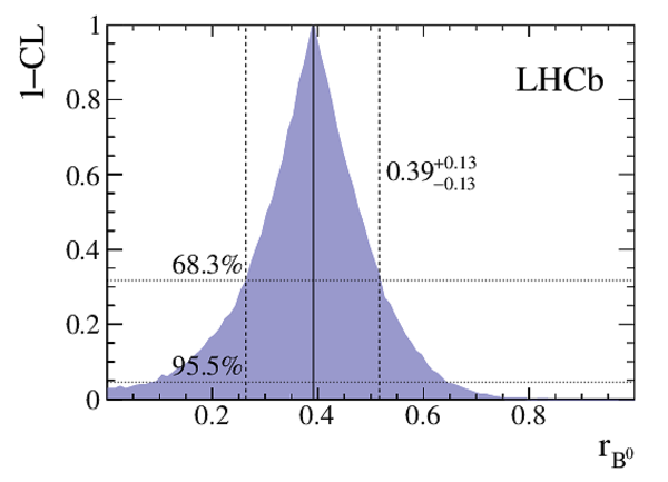
A model-dependent amplitude analysis of the decay $B^0\rightarrow D(K^0_S\pi^+\pi^-) K^{*0}$ is performed using proton-proton collision data corresponding to an integrated luminosity of 3.0fb$^{-1}$, recorded at $\sqrt{s}=7$ and $8 TeV$ by the LHCb experiment. The CP violation observables $x_{\pm}$ and $y_{\pm}$, sensitive to the CKM angle $\gamma$, are measured to be \begin{eqnarray*} x_- &=& -0.15 \pm 0.14 \pm 0.03 \pm 0.01, y_- &=& 0.25 \pm 0.15 \pm 0.06 \pm 0.01, x_+ &=& 0.05 \pm 0.24 \pm 0.04 \pm 0.01, y_+ &=& -0.65^{+0.24}_{-0.23} \pm 0.08 \pm 0.01, \end{eqnarray*} where the first uncertainties are statistical, the second systematic and the third arise from the uncertainty on the $D\rightarrow K^0_S \pi^+\pi^-$ amplitude model. These are the most precise measurements of these observables. They correspond to $\gamma=(80^{+21}_{-22})^{\circ}$ and $r_{B^0}=0.39\pm0.13$, where $r_{B^0}$ is the magnitude of the ratio of the suppressed and favoured $B^0\rightarrow D K^+ \pi^-$ decay amplitudes, in a $K\pi$ mass region of $\pm50 MeV$ around the $K^*(892)^0$ mass and for an absolute value of the cosine of the $K^{*0}$ decay angle larger than $0.4$.
Figures and captions
|
Variation of signal efficiency across the phase space for (left) long and (right) downstream candidates. |
Fig1_left.eps [698 KiB] HiDef png [1 MiB] Thumbnail [427 KiB] *.C file |

|
|
Fig1_right.eps [724 KiB] HiDef png [1 MiB] Thumbnail [432 KiB] *.C file |
|
|
|
Invariant mass distribution for $ B ^0 \rightarrow D K ^{*0} $ long and downstream candidates. The fit result, including signal and background components, is superimposed (solid blue). The points are data, and the different fit components are given in the legend. The two vertical lines represent the signal region in which the $ C P$ fit is performed. |
Fig2.eps [33 KiB] HiDef png [370 KiB] Thumbnail [265 KiB] *.C file |

|
|
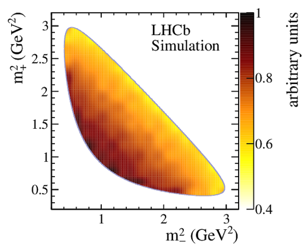
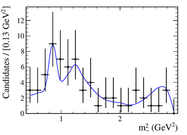
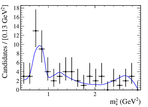
Selected $ B ^0 \rightarrow D K ^{*0} $ candidates, shown as (a) the Dalitz plot, and its projections on (b) $ m^2_-$ , (c) $ m^2_+$ and (d) $ m^2_0$ {}. The line superimposed on the projections corresponds to the fit result and the points are data. |
Fig3a.eps [80 KiB] HiDef png [174 KiB] Thumbnail [128 KiB] *.C file |

|
|
Fig3b.eps [11 KiB] HiDef png [135 KiB] Thumbnail [114 KiB] *.C file |
|
|
|
Fig3c.eps [11 KiB] HiDef png [132 KiB] Thumbnail [121 KiB] *.C file |
|
|
|
Fig3d.eps [11 KiB] HiDef png [130 KiB] Thumbnail [120 KiB] *.C file |

|
|
|
Selected $\overline{ B }{} {}^0 \rightarrow D \overline{ K }{} {}^{*0} $ candidates, shown as (a) the Dalitz plot, and its projections on (b) $ m^2_-$ , (c) $ m^2_+$ and (d) $ m^2_0$ {}. The line superimposed on the projections corresponds to the fit result and the points are data. |
Fig4a.eps [80 KiB] HiDef png [175 KiB] Thumbnail [129 KiB] *.C file |

|
|
Fig4b.eps [9 KiB] HiDef png [137 KiB] Thumbnail [124 KiB] *.C file |

|
|
|
Fig4c.eps [11 KiB] HiDef png [134 KiB] Thumbnail [112 KiB] *.C file |

|
|
|
Fig4d.eps [11 KiB] HiDef png [135 KiB] Thumbnail [114 KiB] *.C file |

|
|
|
Likelihood contours at 68.3% and 95.5% confidence level for $(x_{+},y_{+})$ (red) and $(x_{-},y_{-})$ (blue), obtained from the $ C P$ fit. |
Fig5.eps [7 KiB] HiDef png [171 KiB] Thumbnail [105 KiB] *.C file |

|
|
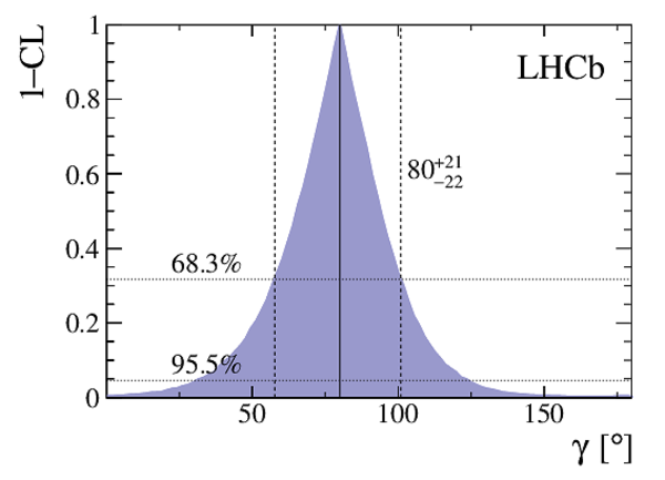
Confidence level curve on $\gamma$ , obtained using the "plugin" method [58]. |
Fig6.eps [60 KiB] HiDef png [177 KiB] Thumbnail [133 KiB] *.C file |
|
|
Confidence level curve on $ r_{ B ^0 }$ , obtained using the "plugin" method [58]. |
Fig7.eps [51 KiB] HiDef png [189 KiB] Thumbnail [144 KiB] *.C file |
|
|
Confidence level curve on $\delta_{ B ^0 }$ , obtained using the "plugin" method [58]. Only the $\delta_{ B ^0 }$ solution corresponding to $0<\gamma <180 ^{\circ} $ is highlighted; the other maximum is due to the $(\delta_{ B ^0 } ,\gamma )\rightarrow (\delta_{ B ^0 } +\pi,\gamma +\pi)$ ambiguity. |
Fig8.eps [62 KiB] HiDef png [211 KiB] Thumbnail [147 KiB] *.C file |

|
|
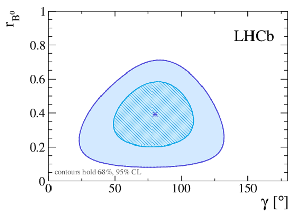
Two-dimensional confidence level curves in the $(\gamma , r_{ B ^0 } )$ plane, obtained using the profile-likelihood method. |
Fig9.eps [12 KiB] HiDef png [338 KiB] Thumbnail [205 KiB] *.C file |
|
|
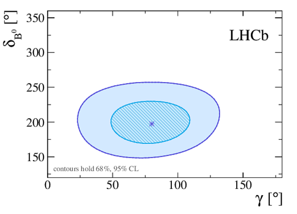
Two-dimensional confidence level curves in the $(\gamma ,\delta_{ B ^0 } )$ plane, obtained using the profile-likelihood method. |
Fig10.eps [11 KiB] HiDef png [280 KiB] Thumbnail [171 KiB] *.C file |
|
|
Animated gif made out of all figures. |
PAPER-2016-007.gif Thumbnail |

|
![HiDef png [1 MiB]](Directory_LHCb-PAPER-2016-007/hidef_Fig1_left.png)
![HiDef png [1 MiB]](Directory_LHCb-PAPER-2016-007/hidef_Fig1_right.png)
![HiDef png [370 KiB]](Directory_LHCb-PAPER-2016-007/hidef_Fig2.png)
![HiDef png [174 KiB]](Directory_LHCb-PAPER-2016-007/hidef_Fig3a.png)
![HiDef png [135 KiB]](Directory_LHCb-PAPER-2016-007/hidef_Fig3b.png)
![HiDef png [132 KiB]](Directory_LHCb-PAPER-2016-007/hidef_Fig3c.png)
![HiDef png [130 KiB]](Directory_LHCb-PAPER-2016-007/hidef_Fig3d.png)
![HiDef png [175 KiB]](Directory_LHCb-PAPER-2016-007/hidef_Fig4a.png)
![HiDef png [137 KiB]](Directory_LHCb-PAPER-2016-007/hidef_Fig4b.png)
![HiDef png [134 KiB]](Directory_LHCb-PAPER-2016-007/hidef_Fig4c.png)
![HiDef png [135 KiB]](Directory_LHCb-PAPER-2016-007/hidef_Fig4d.png)
![HiDef png [171 KiB]](Directory_LHCb-PAPER-2016-007/hidef_Fig5.png)
![HiDef png [177 KiB]](Directory_LHCb-PAPER-2016-007/hidef_Fig6.png)
![HiDef png [189 KiB]](Directory_LHCb-PAPER-2016-007/hidef_Fig7.png)
![HiDef png [211 KiB]](Directory_LHCb-PAPER-2016-007/hidef_Fig8.png)
![HiDef png [338 KiB]](Directory_LHCb-PAPER-2016-007/hidef_Fig9.png)
![HiDef png [280 KiB]](Directory_LHCb-PAPER-2016-007/hidef_Fig10.png)
Tables and captions
|
Signal and background yields in the signal region, $\pm25\mathrm{ Me V} $ around the $ B ^0$ mass, obtained from the invariant mass fit. Total yields, as well as separate yields for long and downstream candidates, are given. |
Table_1.pdf [53 KiB] HiDef png [94 KiB] Thumbnail [45 KiB] tex code |

|
|
Summary of the systematic uncertainties on $ z_{\pm}$ , in units of $(10^{-3})$. The total experimental and total model-related uncertainties are also given as percentages of the statistical uncertainties. |
Table_2.pdf [59 KiB] HiDef png [107 KiB] Thumbnail [49 KiB] tex code |

|
|
Model related systematic uncertainties for each alternative model, in units of $(10^{-3})$. The relative signs indicate full correlation or anti-correlation. |
Table_3.pdf [52 KiB] HiDef png [153 KiB] Thumbnail [73 KiB] tex code |

|
![HiDef png [94 KiB]](Directory_LHCb-PAPER-2016-007/hidef_Table_1.png)
![HiDef png [107 KiB]](Directory_LHCb-PAPER-2016-007/hidef_Table_2.png)
![HiDef png [153 KiB]](Directory_LHCb-PAPER-2016-007/hidef_Table_3.png)
Created on 23 May 2024.