Topology of the signal decay. A requirement on the distance between the 3 $\pi $ and the $ B ^0$ vertices along the beam direction to be greater than four times its uncertainty is applied.

Distribution of the distance between the $ B ^0$ vertex and the 3 $\pi $ vertex along the beam direction, divided by its uncertainty, obtained using simulation. The vertical line shows the 4$\sigma$ requirement used in the analysis to reject the prompt background component.

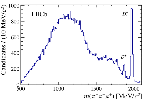
Distribution of the $3\pi$ mass for candidates after the detached-vertex requirement. The $ D ^+$ and $ D ^+_ s $ mass peaks are indicated.

Distribution of the $ K ^- 3\pi$ mass for $D^0$ candidates where a charged kaon has been associated to the 3 $\pi $ vertex.

Distribution of the $ D ^{*-} {3\pi}$ mass (blue) before and (red) after a requirement of finding an energy of at least 8 $\mathrm{ Ge V}$ in the electromagnetic calorimeter around the 3 $\pi $ direction.

Distribution of the $ K ^-$ $\pi ^+$ $\pi ^+$ mass for $D^+$ candidates passing the signal selection, where the negative pion has been identified as a kaon and assigned the kaon mass.

Distribution of the $ D ^{*-} 3\pi$ mass for candidates passing the selection.

Difference between the reconstructed and true $ q^2$ variables divided by the true $ q^2$ , observed in the $ B ^0 \rightarrow D ^{*-} \tau ^+ \nu _\tau $ simulated signal sample after partial reconstruction.

Distribution of the reconstructed $3\pi N$ mass observed in a data sample enriched by $ B \rightarrow D ^{*-} D ^+_ s (X)$ candidates.

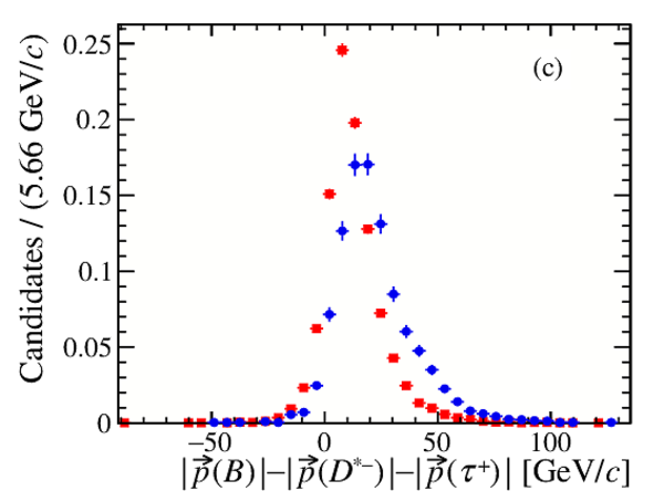
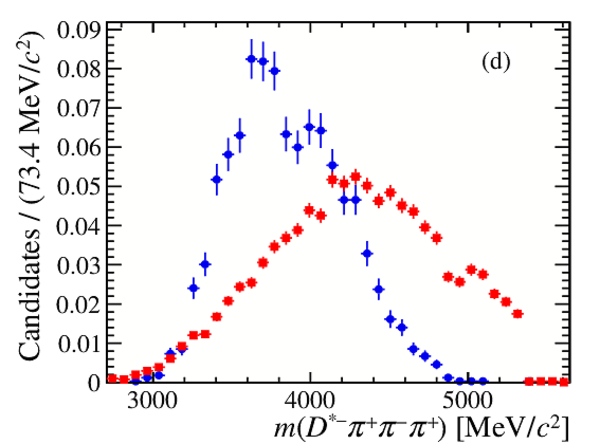
Normalized distributions of (a) $\min[m(\pi^+ \pi^-)]$, (b) $\max[m(\pi^+\pi^-)]$, (c) approximated neutrino momentum reconstructed in the signal hypothesis, and (d) the $D^{*-} 3\pi$ mass in simulated samples.

Distribution of the BDT response on the signal and background simulated samples.

Composition of an inclusive simulated sample where a $ D ^{*-}$ and a 3 $\pi $ system have been produced in the decay chain of a $ b $ $\overline b $ pair from a $pp$ collision. Each bin shows the fractional contribution of the different possible parents of the 3 $\pi $ system (blue from a $ B ^0$ , yellow for other $ b $ hadrons): from signal; directly from the $ b $ hadron (prompt); from a charm parent $ D ^+_ s $ , $ D ^0$ , or $ D ^+$ meson; 3 $\pi $ from a $ B$ and the $ D ^0$ from the other $ B$ ($B1B2$); from $\tau$ lepton following a $ D ^+_ s $ decay; from a $\tau$ lepton following a $D^{**}\tau ^+ \nu _\tau $ decay ($D^{**}$ denotes here any higher excitation of $ D$ mesons). (Top) After the initial selection and the removal of spurious $3\pi$ candidates. (Middle) For candidates entering the signal fit. (Bottom) For candidates populating the last 3 bins of the BDT distribution (cf. Fig. 16).

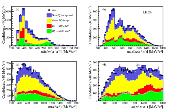
Distributions of (a) ${\mathrm{min}}[m(\pi^+\pi^-)]$, (b) ${\mathrm{max}}[m(\pi^+\pi^-)]$, (c) $m(\pi^+\pi^+)$, (d) $m(\pi^+\pi^-\pi^+)$ for a sample enriched in $ B \rightarrow D ^{*-} D ^+_ s (X)$ decays, obtained by requiring the BDT output below a certain threshold. The different fit components correspond to $ D ^+_ s $ decays with (red) $\eta$ or (green) $\eta ^{\prime} $ in the final state, (yellow) all the other considered $ D ^+_ s $ decays, and (blue) backgrounds originating from decays not involving the $ D ^+_ s $ meson.

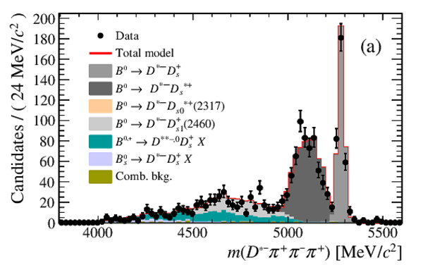
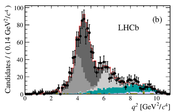
Results from the fit to data for candidates containing a $ D ^{*-}$ $ D ^+_ s $ pair, where $ D ^+_ s \rightarrow 3\pi$. The fit components are described in the legend. The figures correspond to the fit projection on (a) $m(D^{*-}3\pi)$, (b) $q^2$, (c) 3 $\pi $ decay time $t_{\tau}$ and (d) BDT output distributions.

Distribution of $q^2$ for candidates in the $B\rightarrow D^{*-}D^0(X)$ control sample, after correcting for the disagreement between data and simulation.

Projections of the three-dimensional fit on the (a) $3\pi$ decay time, (b) $q^2$ and (c) BDT output distributions. The fit components are described in the legend.

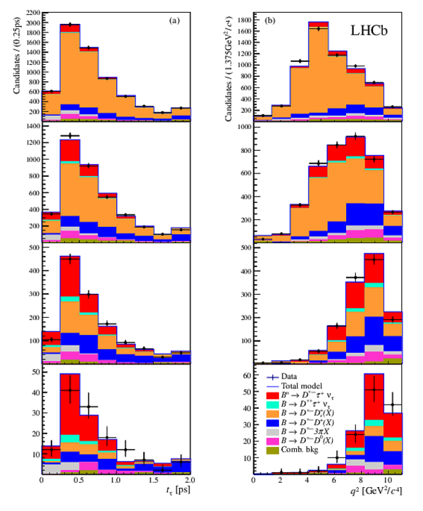
Distributions of (a) $t_{\tau}$ and (b) $q^2$ in four different BDT bins, with increasing values of the BDT response from top to bottom. The fit components are described in the legend.

Projection of the fit results on (a) ${\mathrm{min}}[m(\pi^+\pi^-)]$ and (b) $m(D^{*-}3\pi)$ distributions. The fit components are described in the legend.

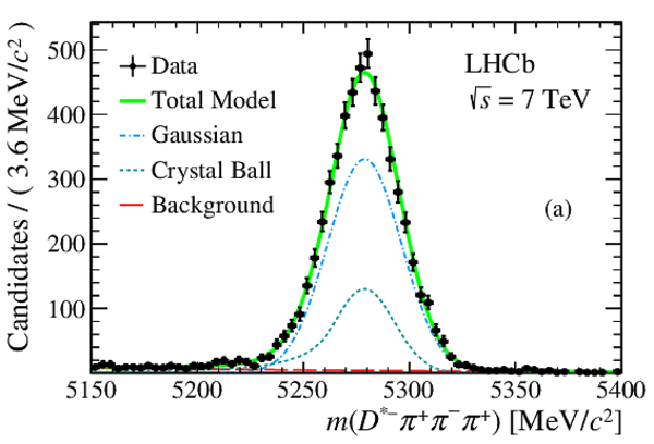
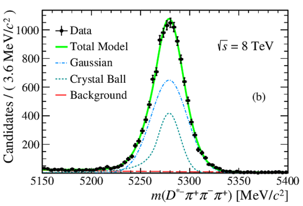
Fit to the $m(D^{*-}3\pi)$ distribution after the full selection in the (a) $\sqrt{s}=7$ TeV and (b) $8$ TeV data samples.

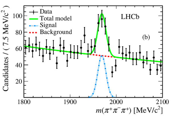
(a) Distribution of $m(3\pi)$ after selection, requiring $m(D^{*-} 3\pi)$ to be between 5200 and 5350 $ {\mathrm{ Me V /}c^2}$ ; (b) fit in the mass region around the $ D ^+_ s $ .

Animated gif made out of all figures.

List of the selection cuts. See text for further explanation.

Summary of the efficiencies (in %) measured at the various steps of the analysis for simulated samples of the $ B ^0 \rightarrow D ^{*-} 3\pi$ channel and the $ B ^0$ $\rightarrow$ $ D ^{*-}$ $\tau ^+$ $\nu _\tau$ signal channel for both $\tau $ decays to 3 $\pi $ $\overline{\nu } _\tau$ and 3 $\pi $ $\pi ^0$ $\overline{\nu } _\tau$ modes. No requirement on the BDT output is applied for $ D ^{*-} 3\pi$ candidates. The relative efficiency designates the individual efficiency of each requirement.

Results of the fit to the $ D ^+_ s $ decay model. The relative contribution of each decay and the correction to be applied to the simulation are reported in the second and third columns, respectively.

Relative fractions of the various components obtained from the fit to the $B\rightarrow D^{*-}D_{s}^{+}(X)$ control sample. The values used in the simulation and the ratio of the two are also shown.

Summary of fit components and their corresponding normalization parameters. The first three components correspond to parameters related to the signal.

Fit results for the three-dimensional fit. The constraints on the parameters $f_{D_s^+}$, $f_{D_{s0}^{*+}}$, $f_{D_{s1}^+}$, $f_{D_s^+X}$ and $f_{(D_s^{+}X)_s}$ are applied taking into account their correlations.

List of the individual systematic uncertainties for the measurement of the ratio $\mathcal{B} ( B ^0 \rightarrow D^{*-}\tau^+\nu_{\tau})/\mathcal{B} ( B ^0 \rightarrow D^{*-}3\pi)$.