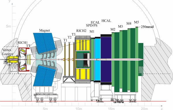
View of the LHCb detector \protec [24].

Average number of visible interactions per bunch crossing ('pile-up', top) and instantaneous luminosity (bottom) at the LHCb interaction point in the period 2010-2012. The dotted lines show the design values.

Development of the instantaneous luminosity for ATLAS, CMS and LHCb during LHC fill 2651. After ramping to the desired value of $4 \times 10^{32}\mathrm{cm^{-2}s^{-1}}$ for LHCb, the luminosity is kept stable in a range of 5% for about 15 hours by adjusting the transversal beam overlap. The difference in luminosity towards the end of the fill between ATLAS, CMS and LHCb is due to the difference in the final focusing at the collision points, commonly referred to as the beta function, $\beta^*$.

Integrated luminosity in LHCb during the three years of LHC Run I. The figure shows the curves for the delivered (dark coloured lines) and recorded (light coloured lines) integrated luminosities.

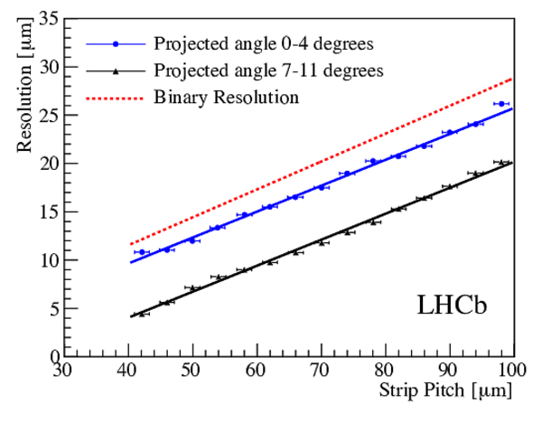
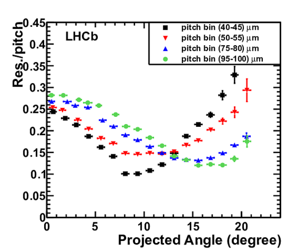
The VELO hit resolution as a function of the inter-strip pitch (left) evaluated with 2010 data for the $R$ sensors. Results are shown for two projected angle ranges and the expected resolution of a single-hit binary system is indicated for comparison. Resolution divided by pitch as a function of the track projected angle for four different strip pitches (right).

The effective depletion voltage versus fluence for all VELO sensors up to the end of LHC Run 1 at 3.4 $ fb^{-1}$ delivered integrated luminosity.

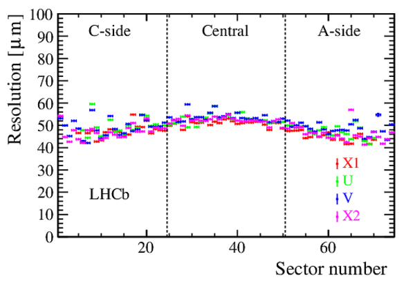
Hit resolution measured for all modules in the TT. The sector number corresponds approximately to the $x$-direction. The resolution improves in the outer regions of the "A-side" and "C-side" regions where there is more charge sharing due to the larger track angle. It is almost constant in the sectors in the "Central" region where the occupancy is highest. The labels $X1$, $U$, $V$ and $X2$ correspond to the four detection layers arranged with an $(x-u-v-x)$ geometry in the TT box.

Hit resolution measured for modules in IT1 (bottom), IT2 (middle) and IT3 (top). The sector number corresponds approximately to the $x$-direction. The resolution in the 1-sensor sectors in the boxes above (Top) and below (Bottom) the beam-pipe are constant. The resolution improves for the 2-sensor sectors in the A- and C-side boxes with increasing distance from beam-pipe where the track angle is typically larger. The labels $X1$, $U$, $V$ and $X2$ correspond to the four detection layers arranged with an $(x-u-v-x)$ geometry in each box.

Drift time distribution (left) for the modules located closest to the beam ("M8"). Drift time versus distance relation (right) where the red-dotted lines indicate the centre and the edge of the straw, corresponding to drift times of 0 and 36 ns, respectively \protec [32].

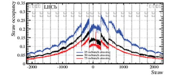
Straw occupancy for (red) $75 \mathrm{ns}$, (black) $50 \mathrm{ns}$ and (blue) $25 \mathrm{ns}$ bunch-crossing spacing, for comparable pile-up conditions \protec [32]. The modules are indicated by 'M', and contain 256 straws each. The width of the module is 340 mm.

Example of the OT efficiency profile as a function of the distance between the extrapolated track position and the centre of the straw for hits in the detector modules on either side of the beam-pipe (type M7) \protec [32]. The vertical bars represent the edges of the straw cell.

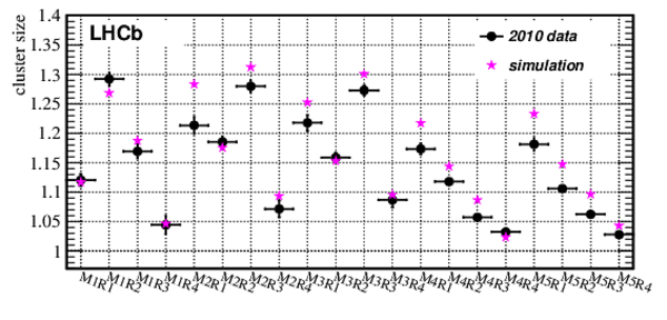
Average cluster size in each detector region for data and simulation \protec [35]. The labels refer to the stations (M1 to M5) and to the four regions with different granularity used in each station (from the innermost R1 to the outermost R4) . Only isolated muon tracks are used, and angular effects are corrected for.

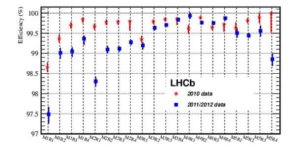
Average measured hit efficiency, in percent, for the different regions of the muon detector. Statistic and systematic uncertainties are added in quadrature. The effect of the few known dead channels is not included. Measurement in the 2010 and 2011/2012 data taking periods are shown separately due to different pile-up conditions.

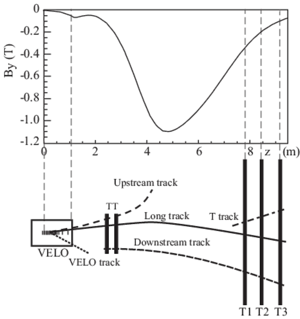
A schematic illustration of the various track types \protec [25]: long, upstream, downstream, VELO and T tracks. For reference the main $B$-field component ($B_y$) is plotted above as a function of the $z$ coordinate.

Display of the reconstructed tracks and assigned hits in an event in the $x$-$z$ plane \protec [25]. The insert shows a zoom into the VELO region in the $x$-$y$ plane.

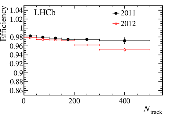
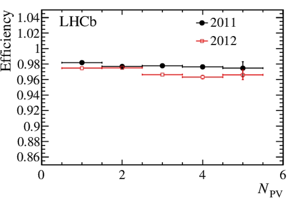
Tracking efficiency as function of the momentum, $p$, the pseudorapidity, $\eta$, the total number of tracks in the event, $N_{\rm track}$, and the number of reconstructed primary vertices, $N_{\rm PV}$ \protec [50]. The error bars indicate the statistical uncertainty.

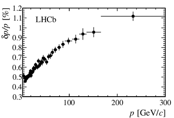
Relative momentum resolution versus momentum for long tracks in data obtained using $ { J \mskip -3mu/\mskip -2mu\psi \mskip 2mu}$ decays.

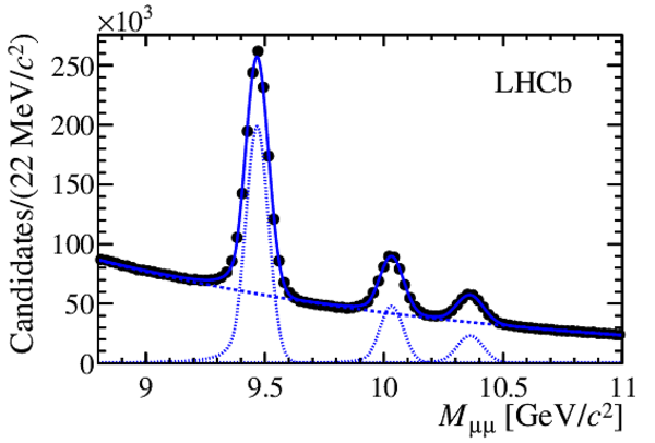
Mass distributions for (top left) $ { J \mskip -3mu/\mskip -2mu\psi \mskip 2mu}$ , (top right) $\psi {(2S)}$ , (bottom left) \Y1S, \Y2S and \Y3S, and (bottom right) $ Z ^0$ candidates. The shapes from the mass fits are superimposed, indicating the signal component (dotted line), the background component (dashed line) and the total yield (solid line).

Mass resolution ($\sigma_m$) (left) and relative mass resolution (right) as a function of the mass ($m$) of the dimuon resonance. The mass of the muons can be neglected in the invariant mass calculation of these resonances. The mass resolution is obtained from a fit to the mass distributions. The superimposed curve is obtained from an empirical power-law fit through the data points.

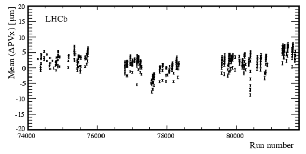
Run dependence of the relative misalignment of the two VELO {} halves along the $x$ axis evaluated with primary vertices.

IP$_x$ resolution as a function of $1/p_{\rm T}$ , comparing different qualities of alignment, measured on 2010 data.

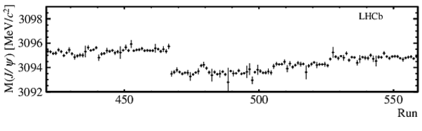
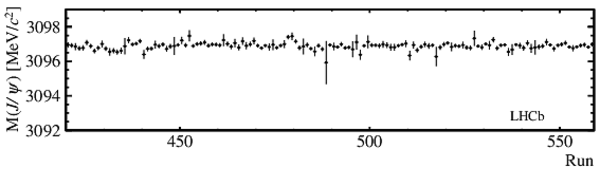
Fitted position of the peak of the $ { J \mskip -3mu/\mskip -2mu\psi \mskip 2mu} \rightarrow \mu ^+\mu ^- $ invariant mass distribution as a function of run number in a two-week period in which the operating temperature of TT modules was varied. The mass is evaluated using the same alignment for the full period on the top and using a dedicated track alignment for each period with constant temperature on the bottom.

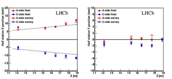
Alignment of the ten muon half stations for the 2012 run. The values of the inner edge in the $x$ position (left) and of the median $y$ position are shown as a function of the station position along $z$. The empty and full dots represent the results from the survey measurements and the software alignment respectively. The error bars, when visible, show the sum in quadrature of statistic and systematic uncertainties.The dashed lines represent the ideal projective alignment of the detector in the closed position.

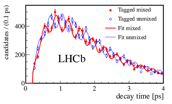
Decay time distribution for $ B ^0_ s \rightarrow D_s^- \pi^+$ candidates tagged as mixed (different flavour at decay and production; red, continuous line) or unmixed (same flavour at decay and production; blue, dotted line) \protec [66].

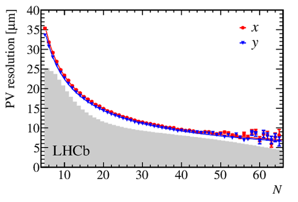
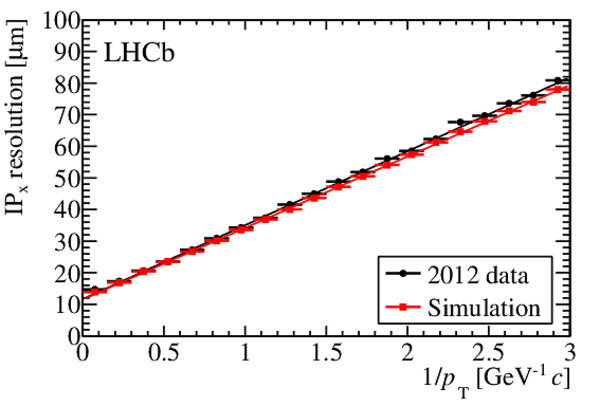
The primary vertex resolution (left), for events with one reconstructed primary vertex, as a function of track multiplicity. The $x$ (red) and $y$ (blue) resolutions are separately shown and the superimposed histogram shows the distribution of number of tracks per reconstructed primary vertex for all events that pass the high level trigger. The impact parameter in $x$ resolution as a function of $1/p_{\rm T}$ (right). Both plots are made using data collected in 2012.

Decay time resolution as a function of momentum (left) and as a function of the estimated decay time uncertainty (right) of fake, prompt $ B ^0_ s \rightarrow { J \mskip -3mu/\mskip -2mu\psi \mskip 2mu} \phi\rightarrow \mu ^+\mu ^- K ^+ K ^- $ candidates in 2011 and 2012 data. Only events with a single reconstructed primary vertex are used. The superimposed histogram shows the distribution of momentum (left) and estimated decay time uncertainty (right) on an arbitrary scale.

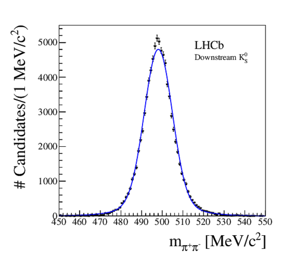
Distribution of the invariant mass of $ K ^0_{\rm\scriptscriptstyle S} \rightarrow \pi ^+\pi ^- $ candidates with a decay vertex at a significant distance to the PV, for long tracks (left) and downstream tracks (right). A mass resolution of $3.5$ $ {\mathrm{ Me V /}c^2}$ is achieved for the candidates reconstructed from long tracks and $7$ $ {\mathrm{ Me V /}c^2}$ for those using downstream tracks.

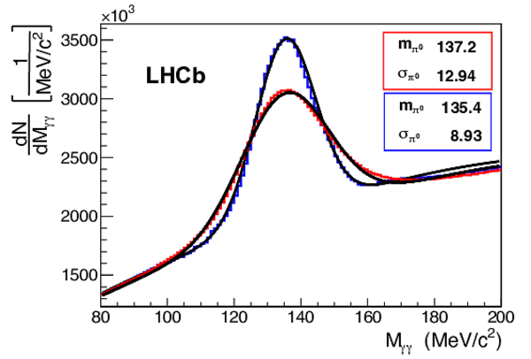
Invariant mass distribution for $\pi ^0 \rightarrow \gamma\gamma$ candidates upon which the fine calibration algorithm is applied. The red curve corresponds to the distribution before applying the method, while the blue curve is the final one. Values in the red (blue) box are the mean and sigma of the signal peak distribution in $ {\mathrm{ Me V /}c^2}$ before (after) applying the fine calibration method.

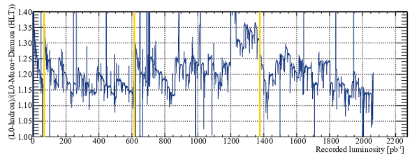
Ratio between the rate of events triggered by the L0-hadron trigger, based on the HCAL, and Muon-based triggers. Distinct increases in rate, e.g. as at a recorded luminosity of around 50 $ pb^{-1}$ , correspond to the application of a new set of PMT gains.

Mass distribution of reconstructed $B^0\rightarrow K^{*0}(K^+ \pi^-)\gamma$ candidates obtained in the 2011 data sample. The blue curve corresponds to the mass shape fit. The $K^{*0}\gamma$ signal (green dotted line) and the various background contaminations are shown \protec [78].

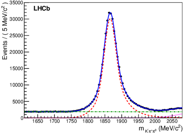
Mass distributions of reconstructed {$D^0\rightarrow K^-\pi^+ \pi^0$} candidates with resolved $\pi^0$ (left) and merged $\pi^0$ (right). Both are obtained from the 2011 data sample. The overall mass fit \protec [79] is represented by the blue curve, with the signal (red dashed line) and background (green dash-dotted line and purple dotted lines) contributions also shown.

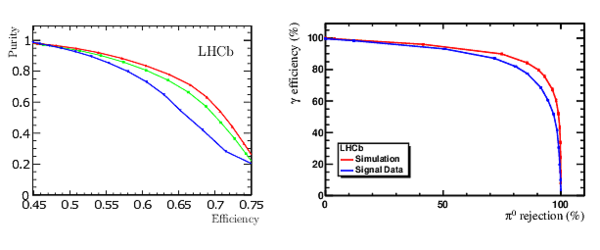
Performance of the photon identification. Purity as a function of efficiency for (green) the full photon candidate sample, (blue) converted candidates according to the SPD information and (red) non-converted candidates (left). Photon identification efficiency as a function of $\pi ^0$ rejection efficiency for the $\gamma-\pi ^0 $ separation tool for simulation, the red curve, and data, the blue curve (right).

Ratio of photon detection efficiencies $\epsilon (\gamma \rightarrow e^+e^-)/\epsilon(\gamma_\text{CALO})$ from the decay of $\pi ^0$ mesons in data (red) and simulations (blue).

Distribution for the ECAL of E/pc for electrons (red) and hadrons (blue), as obtained from the first 340 $ pb^{-1}$ recorded in 2011.

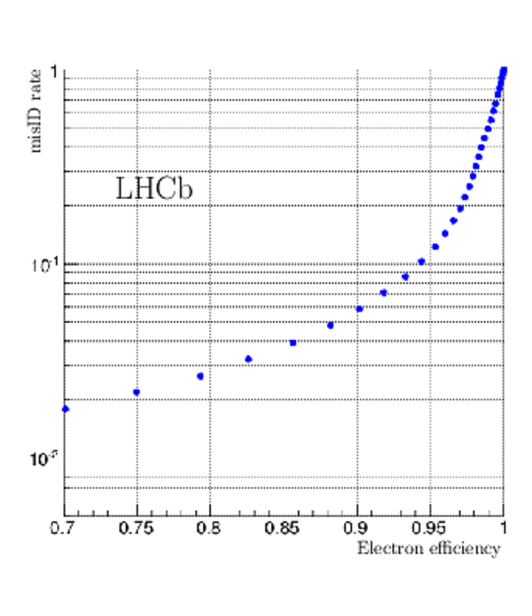
Electron identification efficiency versus misidentification rate.

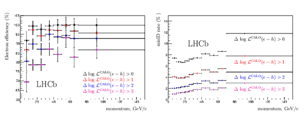
Electron identification performances for various $\Delta$ log ${\mathcal L}^\text{CALO}(e-h)$ cuts: electron efficiency (left) and misidentification rate (right) as functions of the track momentum.

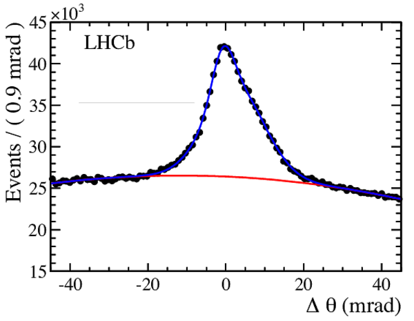
$\Delta\theta_C$ distributions for the RICH 1 gas (top left), RICH 2 gas (top right) and Aerogel (bottom)\protec [82].

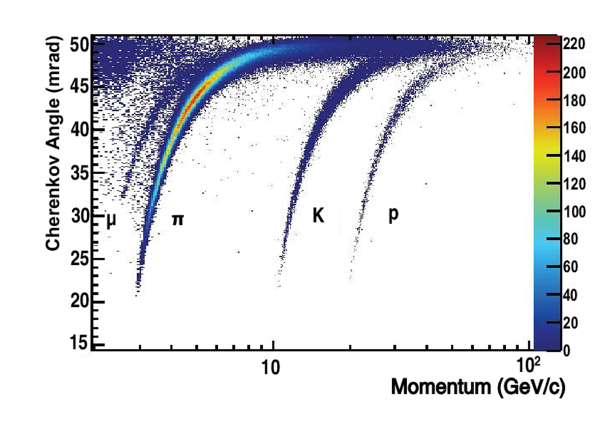
Reconstructed Cherenkov angle for isolated tracks, as a function of track momentum in the $\rm C_4 F_{10}$ radiator \protec [82]. The Cherenkov bands for muons, pions, kaons and protons are clearly visible.

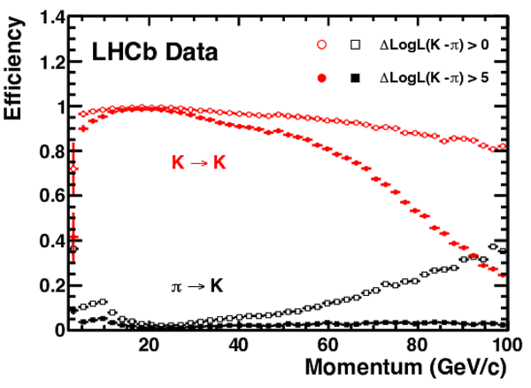
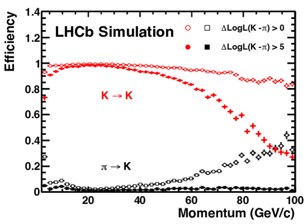
Kaon identification efficiency and pion misidentification rate as measured using data (left) and from simulation (right) as a function of track momentum\protec [82]. Two different $\rm \Delta log \mathcal{L}(K-\pi)$ requirements have been imposed on the samples, resulting in the open and filled marker distributions, respectively.

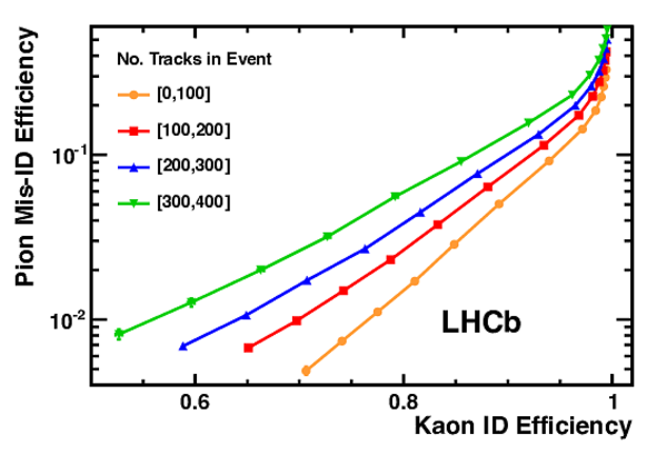
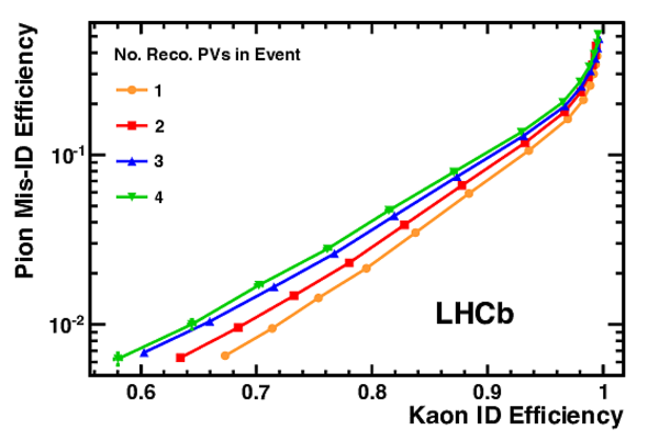
Pion misidentification fraction versus kaon identification efficiency as measured in 7 TeV LHCb collisions: (left) as a function of track multiplicity, and (right) as a function of the number of reconstructed primary vertices \protec [82]. The efficiencies are averaged over all particle momenta.

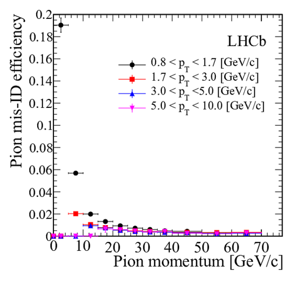
Top left: efficiency of the muon candidate selection based on the matching of hits in the muon system to track extrapolation, as a function of momentum for different $p_{\rm T}$ ranges. Other panels: misidentification probability of protons (top right), pions (bottom left), and kaons (bottom right) as muon candidates as a function of momentum, for different $p_{\rm T}$ ranges.

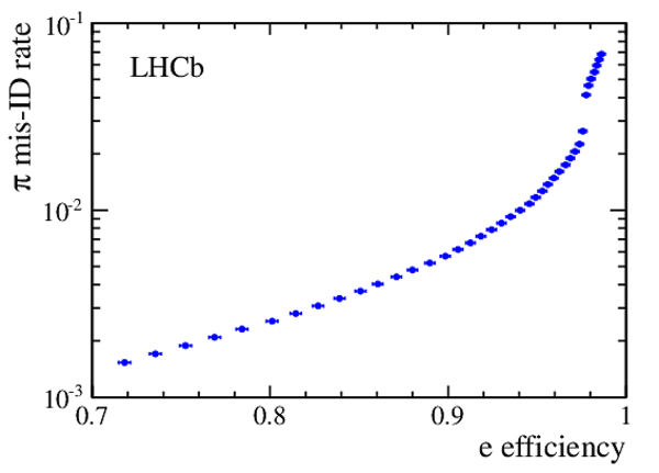
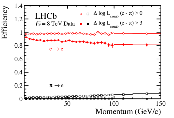
Electron identification performance using the $ \Delta {\rm log} {\mathcal L}_{comb} (e-\pi) $ variable, as measured in 8 TeV collision data, using a tag and probe technique with electrons from the decay $B^{\pm} \rightarrow (J/\psi \rightarrow e^+e^-) K^{\pm}$. Left, pion misidentication rate versus electron identification probability when the cut value is varied. Right, electron identification efficiency and pion misidentification rate as a function of track momentum, for two different cuts on $ \Delta {\rm log} {\mathcal L}_{comb} (e-\pi) $.

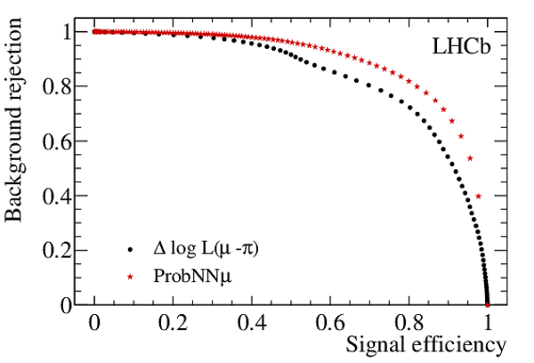
Background misidentification rates versus muon (left) and proton (right) identification efficiency, as measured in the $\Sigma^+\rightarrow p\mu^+\mu^-$ decay study. The variables $ \Delta {\rm log} {\mathcal L} (X-\pi) $ (black) and ProbNN (red), the probability value for each particle hypothesis, are compared for $5-10$ $ {\mathrm{ Ge V /}c}$ muons and $5-50$ $ {\mathrm{ Ge V /}c}$ protons, using data sidebands for backgrounds and Monte Carlo simulation for the signal.

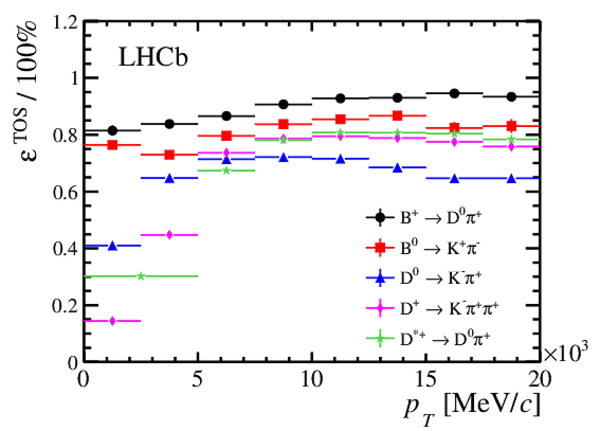
(left) L0 muon trigger performance: TOS trigger efficiency for selected $ B ^+ \rightarrow { J \mskip -3mu/\mskip -2mu\psi \mskip 2mu} K ^+ $ candidates. (right) L0 hadron trigger performance: TOS trigger efficiency for different beauty and charm decay modes.

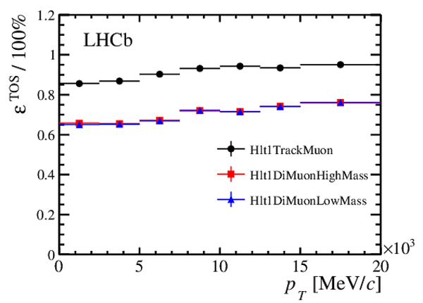
HLT1 inclusive track trigger performance: TOS efficiency for various channels as a function of $ B $ or $ D $ $p_{\rm T}$ (left) . HLT1 muon trigger performance : TOS efficiency for $ B ^+ \rightarrow { J \mskip -3mu/\mskip -2mu\psi \mskip 2mu} K ^+ $ candidates as function of $ B ^+$ $p_{\rm T}$ (right).

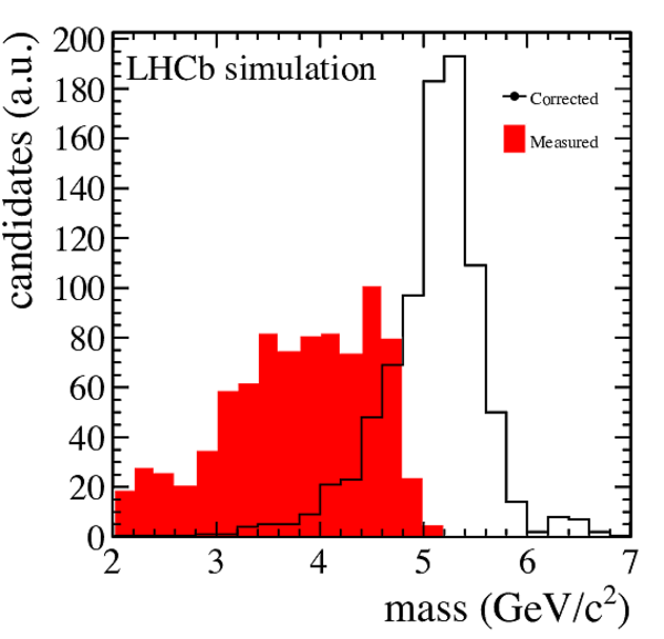
Simulated $ B ^0 \rightarrow K ^{*0} \mu ^+ \mu ^- $ events. The reconstructed 2-body mass is shown in red and the corrected mass ($m_{\rm corr}$, see text for definition) is shown in black.

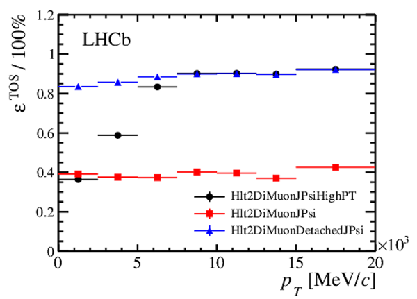
HLT2 muon trigger performance for the $ { J \mskip -3mu/\mskip -2mu\psi \mskip 2mu}$ trigger lines (left). The triggers \texttt{Hlt2DiMuonJPsi} and \texttt{Hlt2DiMuonJPsiHighPT} are the two prompt $ { J \mskip -3mu/\mskip -2mu\psi \mskip 2mu}$ triggers and \texttt{Hlt2DiMuonDetachedJPsi} is the trigger that selects $ { J \mskip -3mu/\mskip -2mu\psi \mskip 2mu}$ candidates that are inconsistent with coming from the primary vertex. HLT2 charm trigger performance for inclusive and exclusive selections (right). The decay $D^{*+} \rightarrow D^0 \pi^+$ is followed by $D^0 \rightarrow K^- \pi^+\pi^+\pi^-$.

Animated gif made out of all figures.

Summary of the hit efficiency and resolution measurements made using 2011 and 2012 data. Results are also shown for simulated events.

Mass resolution for the six different dimuon resonances.

Comparison of photoelectron yields ( $ N_{\rm pe}$ ) determined from $ D ^{*+}\rightarrow D ^0 \pi^+$ decays in simulation and data, and $ p \thinspace p \rightarrow p \thinspace p \thinspace \mu^+ \mu^-$ events in data.

Typical L0 thresholds used in Run I \protec [86].

Efficiencies of selected channels for the whole trigger chain using the 2012 trigger configuration. The efficiencies are normalised to the number of events that are offline selected.