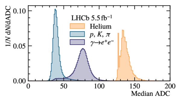
Left: Distributions of the deposited energy in a VELO sensor for simulated helium and protons. Right: Distributions of the median ADC of all VELO clusters per track, corrected for the incidence angle, for $Z=1$ particles (blue), { $ e ^+$ $ e ^-$ pairs} from photon conversions (purple), and helium (orange). The helium selection, described in the text, is applied but no VELO requirements are imposed.

Distributions of the number of overflows for simulated helium signal and $Z=1$ particles from calibration data . The vertical line indicates the preselection requirement.

Distributions of the cluster amplitudes, for different cluster sizes, in the $ {\rm VELO } R$ sensors for (left) simulated helium signal and (right) calibration data .

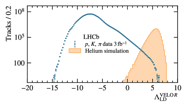
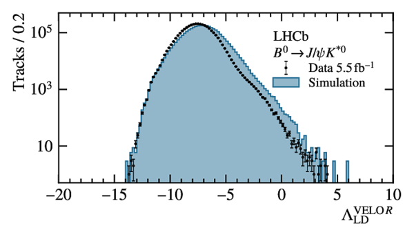
Distributions of $\Lambda_{\rm LD}^{{\rm VELO } R}$ in: (left) samples of $Z=1$ tracks from calibration data and simulated helium; (right) samples of hadrons from $ B ^0 \rightarrow K ^{*0} ( K ^+ \pi ^- ) J/\psi(\mu^+ \mu^-)$ decays. The simulation is normalised to the data.

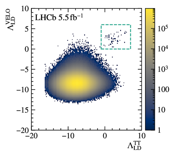
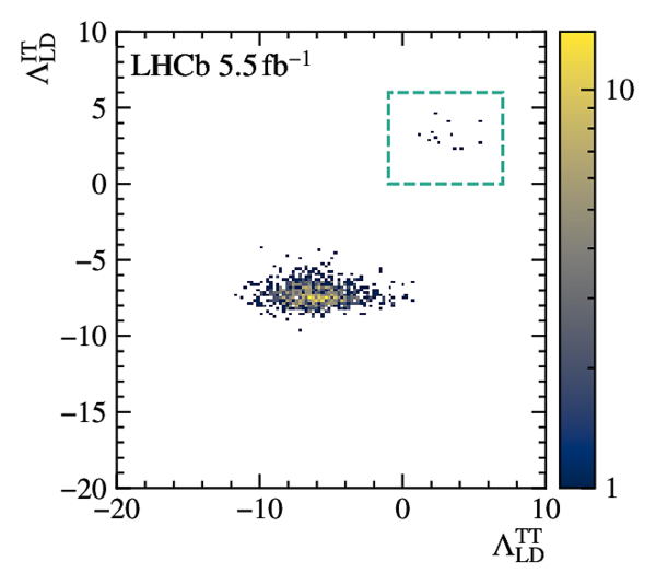
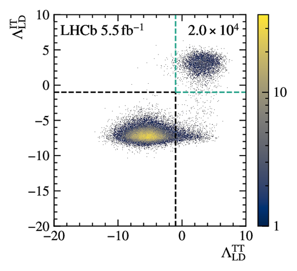
Distributions of the log-likelihood estimators from the LHCb VELO ( $\Lambda_{\rm LD}^{\rm VELO }$ ), TT ( $\Lambda_{\rm LD}^{\rm TT }$ ) and IT ( $\Lambda_{\rm LD}^{\rm IT }$ ) silicon trackers from the minimum-bias data. {Helium candidates are indicated by green boxes.} Left: the tracks are required to pass the selection described in \Cref{sec:tracktime} or to have $\Lambda_{\rm LD}^{\rm IT } >-1$. Right: the tracks must traverse the IT and have $\Lambda_{\rm LD}^{\rm VELO } >0$. The full selection described in \Cref{sec:tracktime,sec:photons,sec:ipchisq} is applied.

Left: Efficiency matrix of the two preselections determined from the helium candidates selected in minimum-bias data. Right: Distribution of the number of overflows in helium candidate tracks from minimum-bias data and $Z=1$ particles from calibration data . The latter is normalised to 25% of the former. The requirement used in the preselection is shown {by the vertical dashed line}.

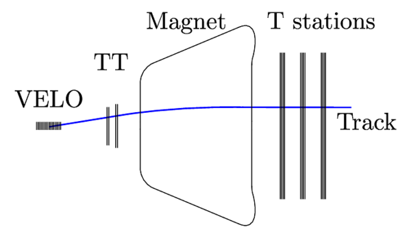
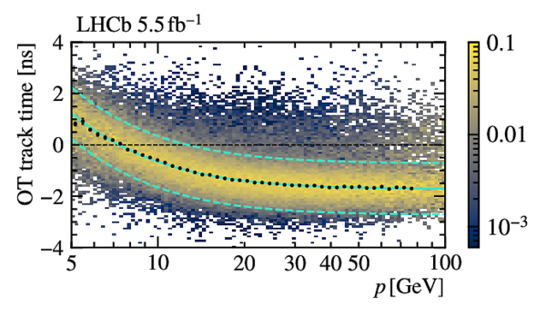
{Left: sketch of the LHCb tracking detectors and magnet; adapted from Ref. [12]. Right:} Distribution of the reference track time versus the momentum for tracks with $\Lambda_{\rm LD}^{\rm VELO } >0$ and $\Lambda_{\rm LD}^{\rm TT } >1$. In each momentum slice, the distribution is normalised to unity and fitted with a Gaussian function. The positions of the means is indicated by the black dots. These are fitted as described in the main body, resulting in the shape depicted by the green continuous line. The {dashed} green lines indicate the $\pm 1$ $\text{ ns}$ interval.

Distribution of the RICH electron-pion separation estimator ( $\Lambda_{e-\pi}^{\rm RICH}$ ) for helium signal and background below the rigidity thresholds for Cherenkov photon production by $ ^3{\rm He}$ in the two LHCb RICH detectors. The vertical dashed line indicates the selection requirement.

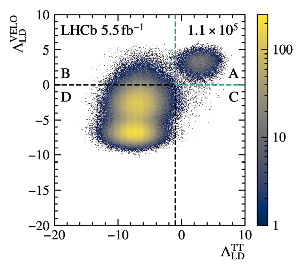
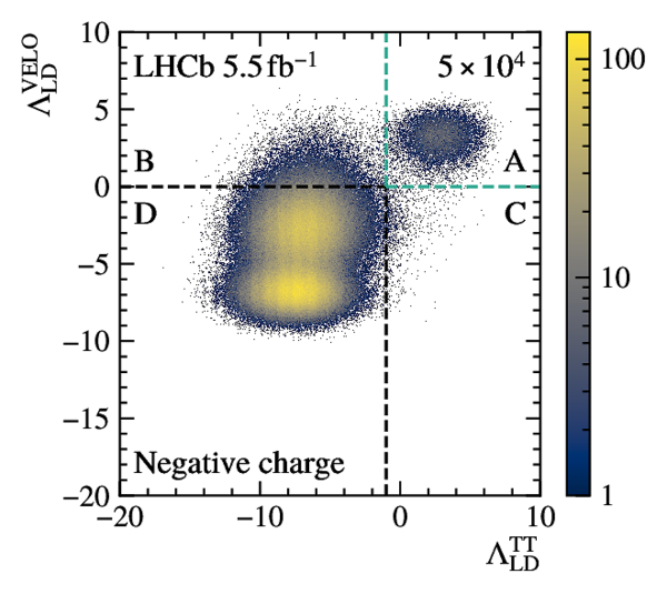
Distributions of the log-likelihood estimators from the LHCb VELO ( $\Lambda_{\rm LD}^{\rm VELO }$ ), TT ( $\Lambda_{\rm LD}^{\rm TT }$ ) and IT ( $\Lambda_{\rm LD}^{\rm IT }$ ) silicon trackers. Left: the tracks are required to pass the downstream selection. Right: the tracks must traverse the IT and have $\Lambda_{\rm LD}^{\rm VELO } >0$. On the left, the signal region is denoted by A, whilst regions B, C, and D correspond to background.

Distributions corresponding to that on the left-hand side of \Cref{fig:LLDsABCD}, but separated into tracks of (left) positive and (right) negative charge.

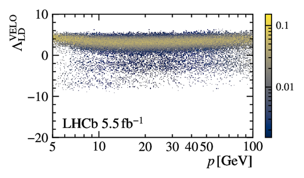
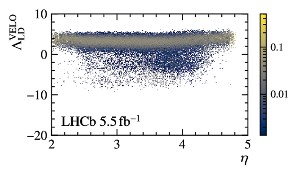
Distribution of $\Lambda_{\rm LD}^{\rm VELO }$ as a function of momentum (left) and pseudorapidity (right), in data from both preselections combined. Tracks are required to pass the selection in \Cref{sec:tracktime}, as well as $\Lambda_{\rm LD}^{\rm TT } >-1$. Each vertical slice is normalised to unity.

Distribution of the natural logarithm of the $\chi^2_{\text{IP}}$ for helium and antihelium tracks, combining data from both preselections. The requirement that separates prompt and displaced helium is shown {by the vertical dashed line}.

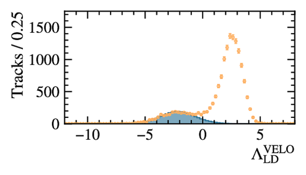
Distribution of $\Lambda_{\rm LD}^{\rm VELO }$ in (left) helium and (right) antihelium samples from the (upper) preselection 2 and (lower) preselection 1 data samples. The distribution from an independent background sample is shown in blue, scaled to match the size of the populations found in data at negative $\Lambda_{\rm LD}^{\rm VELO }$ values. To visualise the background in the preselection 1 sample, the inset of each bottom-row plot shows a magnification of the region $\Lambda_{\rm LD}^{\rm VELO } \in[-10, 1]$. Each inset's horizontal axis matches that of the containing plot.

Animated gif made out of all figures.

Helium selection criteria quantified throughout this paper. The logical or is required between the two preselection criteria. Given the complementary acceptances of OT and IT, the logical or is also required between the downstream requirements.