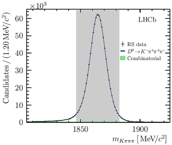
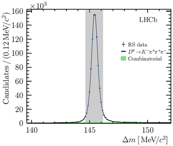
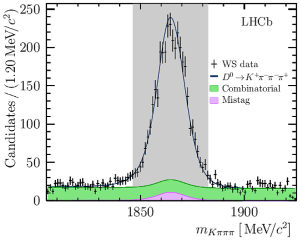
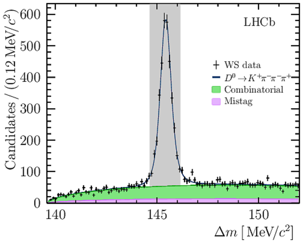
Invariant mass and mass difference distributions for RS (top) and WS (bottom) samples, shown with fit projections. The signal region is indicated by the filled grey area, and for each plot the mass window in the orthogonal projection is applied.

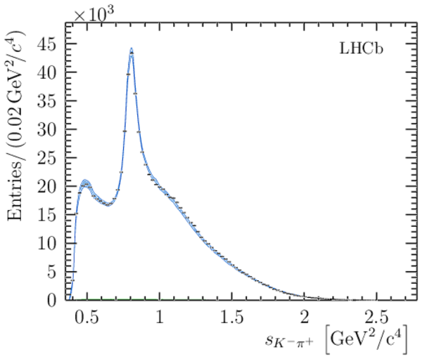
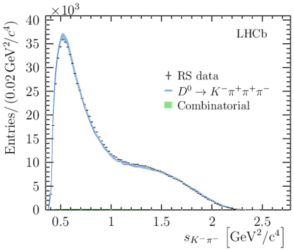
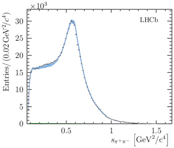
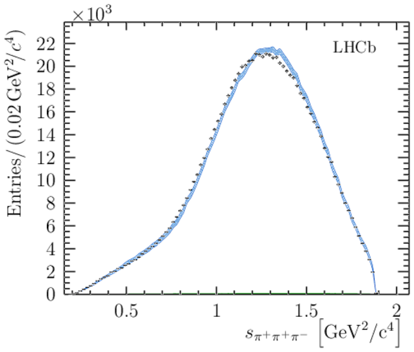
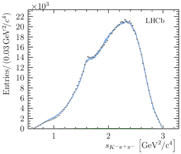
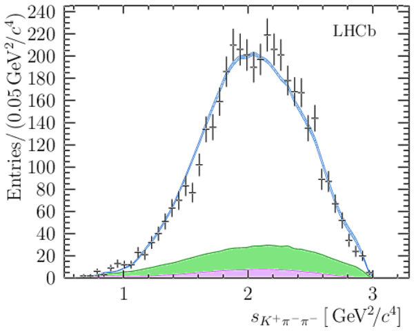
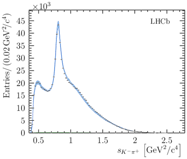
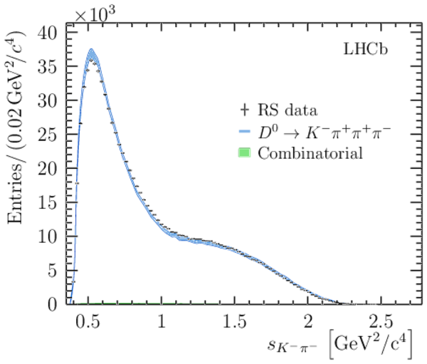
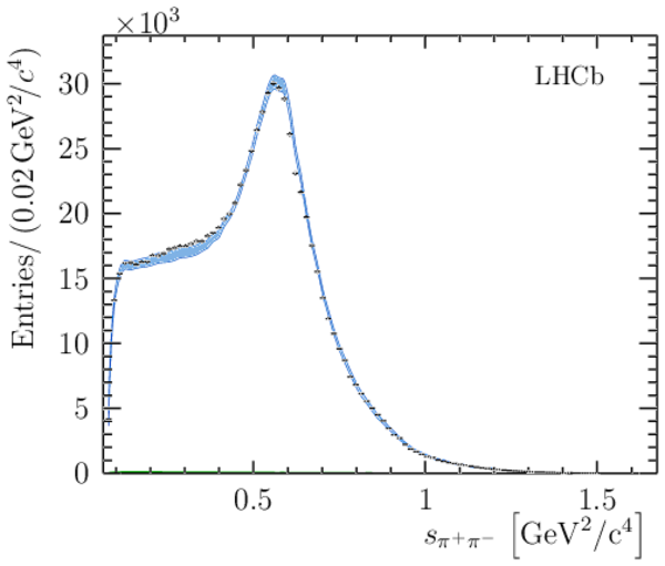
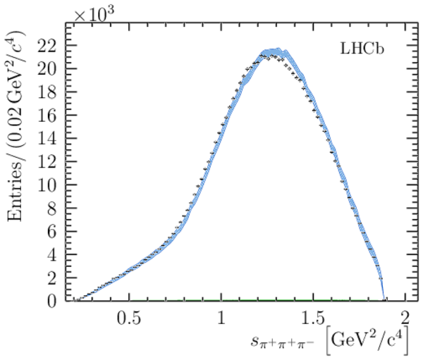
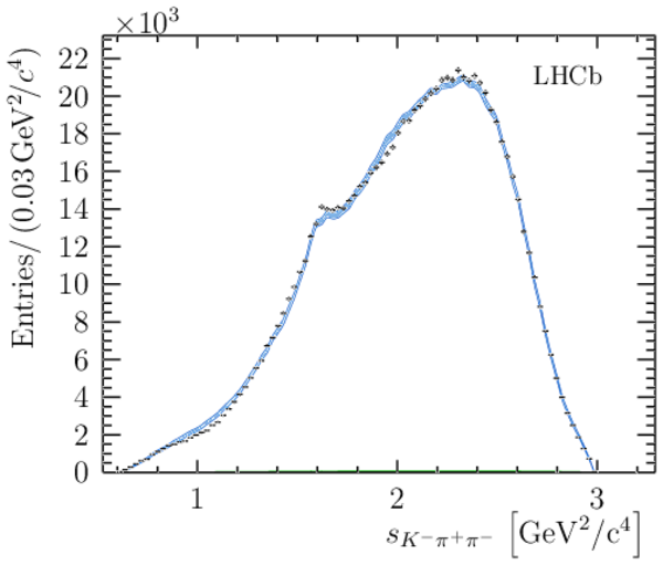
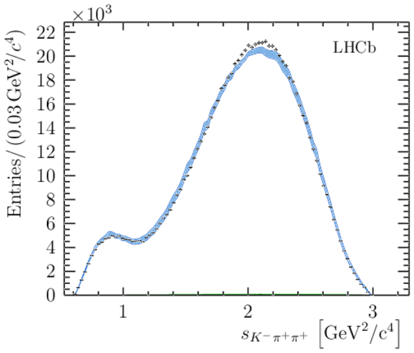
Distributions for six invariant-mass observables in the RS decay $ D ^0 \rightarrow K ^- \pi ^+ \pi ^+ \pi ^- $ . Bands indicate the expectation from the model, with the width of the band indicating the total systematic uncertainty. The total background contribution, which is very low, is shown as a filled area. In figures that involve a single positively-charged pion, one of the two identical pions is selected randomly.

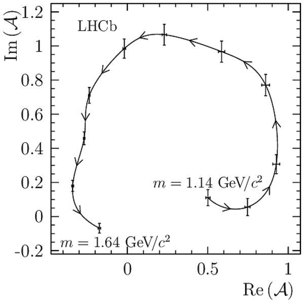
Argand diagram for the model-independent partial-wave analysis (MIPWA) for the $ K (1460)$ resonance. Points show the values of the amplitude that are determined by the fit, with only statistical uncertainties shown.

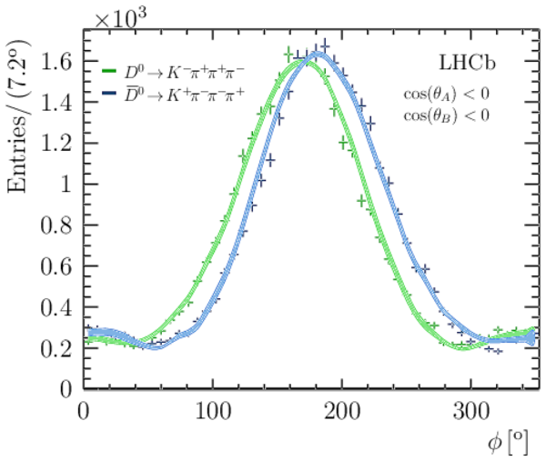
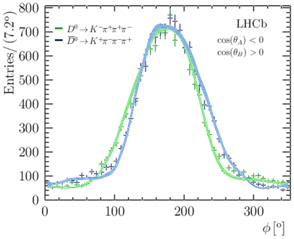
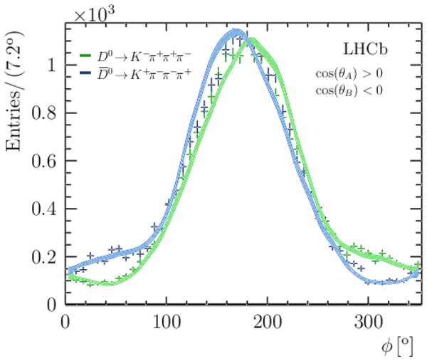
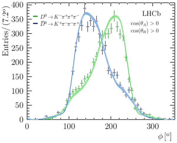
Parity violating distributions for the RS decay in the $\overline{ K }{} {}^* (892)^{0}\rho(770)^{0}$ region defined by $\pm 35 \mathrm{ Me V} $($\pm 100 \mathrm{ Me V} $) mass windows about the nominal $\overline{ K }{} {}^* (892)^{0}$ $(\rho(770)^{0})$ masses. Bands show the predictions of the fitted model including systematic uncertainties.

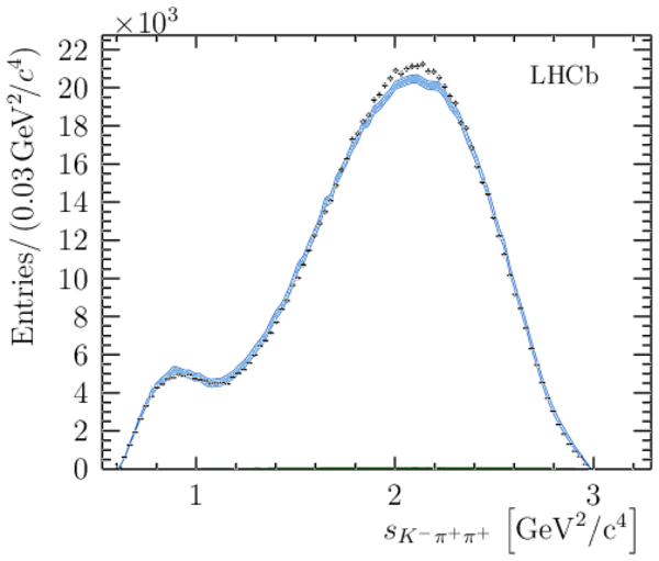
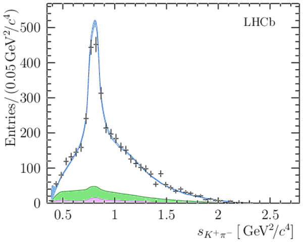
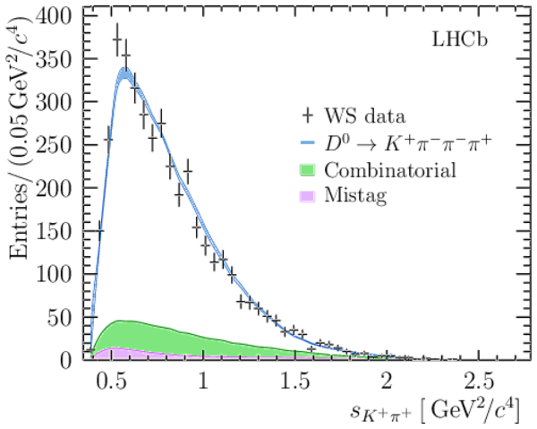
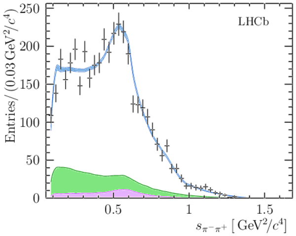
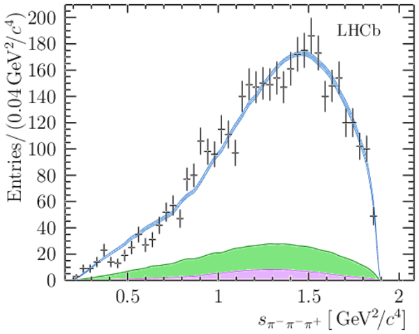
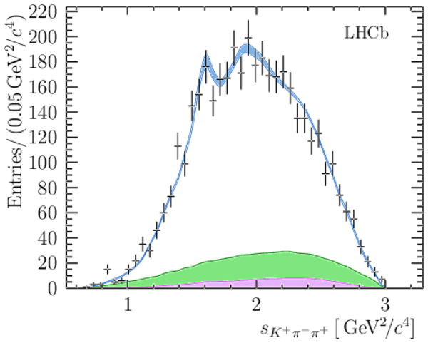
Distributions for six invariant-mass observables in the WS decay $ D ^0 \rightarrow K ^+ \pi ^- \pi ^- \pi ^+ $ . Bands indicate the expectation from the model, with the width of the band indicating the total systematic uncertainty. The total background contribution is shown as a filled area, with the lower region indicating the expected contribution from mistagged $\overline{ D }{} {}^0 \rightarrow K ^+ \pi ^- \pi ^- \pi ^+ $ decays. In figures that involve a single negatively-charged pion, one of the two identical pions is selected randomly.

Distributions for six invariant-mass observables in the RS decay $ D ^0 \rightarrow K ^- \pi ^+ \pi ^+ \pi ^- $ . Bands indicate the expectation from a model which excludes the decay chain $K_1(1270)^{-}\rightarrow \rho(1450)^{0} K ^- $, with the width of the band indicating the total systematic uncertainty. The total background contribution, which is very low, is shown in green.

Animated gif made out of all figures.

Signal and background yields for both samples in the signal region, presented separately for each year of data taking.

Fit fractions and coupling parameters for the RS decay $ D ^0 \rightarrow K ^- \pi ^+ \pi ^+ \pi ^- $ . For each parameter, the first uncertainty is statistical and the second systematic. Couplings $g$ are defined with respect to the coupling to the channel $ D ^0 \rightarrow[\overline{ K }{} {}^* (892)^{0}\rho(770)^{0}]^{L=2}$. Also given are the $\chi^2$ and the number of degrees of freedom ($\nu$) from the fit and their ratio.

Table of fit fractions and coupling parameters for the component involving the $ a_{1}(1260)^{+}$ meson, from the fit performed on the RS decay $ D ^0 \rightarrow K ^- \pi ^+ \pi ^+ \pi ^- $ . The coupling parameters are defined with respect to the $ a_{1}(1260)^{+} \rightarrow\rho(770)^{0}\pi ^+ $ coupling. For each parameter, the first uncertainty is statistical and the second systematic.

Table of fit fractions and coupling parameters for the component involving the $ K_{1}(1270) ^{-}$ meson, from the fit performed on the RS decay $ D ^0 \rightarrow K ^- \pi ^+ \pi ^+ \pi ^- $ . The coupling parameters are defined with respect to the $ K_{1}(1270) ^{-}\rightarrow\rho(770)^{0} K ^- $ coupling. For each parameter, the first uncertainty is statistical and the second systematic.

Table of fit fractions and coupling parameters for the component involving the $ K(1460)^{-}$ meson, from the fit performed on the RS decay $ D ^0 \rightarrow K ^- \pi ^+ \pi ^+ \pi ^- $ . The coupling parameters are defined with respect to the $ K(1460)^{-} \rightarrow\overline{ K }{} {}^* (892)^{0}\pi ^- $ coupling. For each parameter, the first uncertainty is statistical and the second systematic.

Fit fractions and coupling parameters for the WS decay $ D ^0 \rightarrow K ^+ \pi ^- \pi ^- \pi ^+ $ . For each parameter, the first uncertainty is statistical and the second systematic. Couplings $g$ are defined with respect to the coupling to the decay $ D ^0 \rightarrow[ K ^{*}(892)^{0}\rho(770)^{0}]^{L=2}$. Also given are the $\chi^2$ and the number of degrees of freedom ($\nu$) from the fit and their ratio.

Decay chains taken into account in alternative parametrisations of the RS decay mode ${ D ^0 \rightarrow K ^- \pi ^+ \pi ^+ \pi ^- }$. For each chain, the fraction of models in the ensemble that contain this decay, together with the associated average fit fraction, $\langle \mathcal{F} \rangle$, are shown. Components are not tabulated if they contribute to all models in the ensemble, or if they contribute to less than 5% of the models.

Dependence of fit fractions (and partial fractions) on the choice of the RS model. This dependence is expressed as the mean value and the RMS of the values in the ensemble. Also shown is the fit fractions of the baseline model presented in Sect. 6.2.

Dependence of the fitted masses and widths on the final choice of the RS model. This dependence is expressed as the mean value and the RMS of the values in the ensemble. The values found for the baseline model presented in Sect. 6.2 are reported for comparison.

Decay chains taken into account in alternative parametrisations of the WS decay mode ${ D ^0 \rightarrow K ^+ \pi ^- \pi ^- \pi ^+ }$. For each chain, the fraction of models in the ensemble that contain this decay, together with the associated average fit fraction, $\langle \mathcal{F} \rangle$, are shown. Components are not tabulated if they contribute to all models in the ensemble, or if they contribute to less than 5% of the models.

Coherence factor and average strong-phase differences in regions of phase space. The spread of coherence factors, average strong-phase difference and ratio of amplitudes from choice of WS model characterised with the RMS of the distribution.

Rules for calculating the current associated with a given decay chain in terms of the currents of the decay products. Where relevant, the spin projection operator $\mathcal{S}$ and the orbital angular momentum operators $L$ are those for the decaying particle.

Legend for systematic uncertainties, including whether this sources of uncertainty is considered on the RS/WS decay mode.

Systematic uncertainties on the RS decay coupling parameters and fit fractions for quasi two-body decay chains.

Systematic uncertainties on the RS decay coupling parameters, fit fractions and masses and widths of resonances for cascade topology decay chains.

Systematic uncertainties on the WS decay coupling parameters and fit fractions.

Interference fractions for the RS mode $ D ^0 \rightarrow K ^- \pi ^+ \pi ^+ \pi ^- $ , only shown for fractions $>0.5\%$. For each fraction, the first uncertainty is statistical and the second systematic.

Interference fractions for the WS mode $ D ^0 \rightarrow K ^+ \pi ^- \pi ^- \pi ^+ $ , only shown for fractions $>0.5\%$. For each fraction, the first uncertainty is statistical and the second systematic.

Table of fit fractions and coupling parameters and other quantities for the RS decay $ D ^0 \rightarrow K ^- \pi ^+ \pi ^+ \pi ^- $ , for a model excluding the decay chain $K_1(1270)^{-}\rightarrow \rho(1450)^0 K ^- $. Also given is the $\chi^2$ per degree of freedom ($\nu$) for the fit. The first uncertainty is statistical and the second systematic. Couplings are defined with respect to the coupling to the channel $ D ^0 \rightarrow[\overline{ K }{} {}^* (892)^{0}\rho(770)^{0}]^{L=2}$.

Table of fit fractions and coupling parameters for the component involving the $ a_{1}(1260)^{+}$ meson, from the fit performed on the RS decay $ D ^0 \rightarrow K ^- \pi ^+ \pi ^+ \pi ^- $ . The coupling parameters are defined with respect to the $ a_{1}(1260)^{+} \rightarrow\rho(770)^{0}\pi ^+ $ coupling. For each parameter, the first uncertainty is statistical and the second systematic.

Table of fit fractions and coupling parameters for the component involving the $ K_{1}(1270) ^{-}$ meson, from the fit performed on the RS decay $ D ^0 \rightarrow K ^- \pi ^+ \pi ^+ \pi ^- $ . The coupling parameters are defined with respect to the $ K_{1}(1270) ^{-}\rightarrow\rho(770)^{0} K ^- $ coupling. For each parameter, the first uncertainty is statistical and the second systematic.

Table of fit fractions and coupling parameters for the component involving the $ K(1460)^{-}$ meson, from the fit performed on the RS decay $ D ^0 \rightarrow K ^- \pi ^+ \pi ^+ \pi ^- $ . The coupling parameters are defined with respect to the $ K(1460)^{-} \rightarrow\overline{ K }{} {}^* (892)^{0}\pi ^- $ coupling. For each parameter, the first uncertainty is statistical and the second systematic.