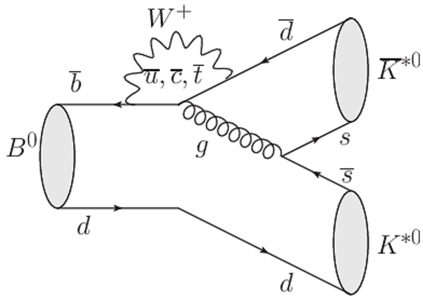
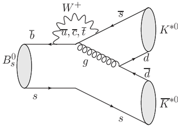
Leading order Feynman diagrams for the $ B ^0 \rightarrow K ^{*0} \overline{ K } {}^{*0} $ and $ B ^0_ s \rightarrow K ^{*0} \overline{ K } {}^{*0} $ decays. Both modes are dominated by a gluonic-penguin diagram.

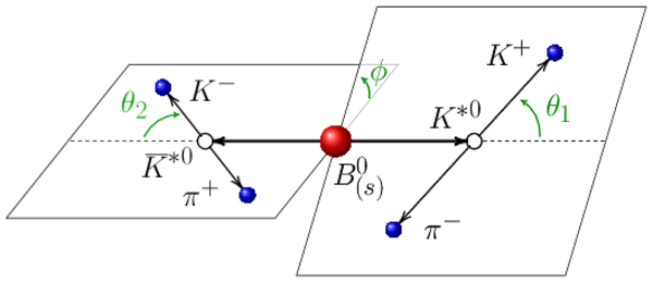
Definition of the helicity angles, employed in the angular analysis of the $ B ^0_{( s )} \rightarrow K ^{*0} \overline{ K } {}^{*0} $ decays. Each angle is defined in the rest frame of the decaying particle.

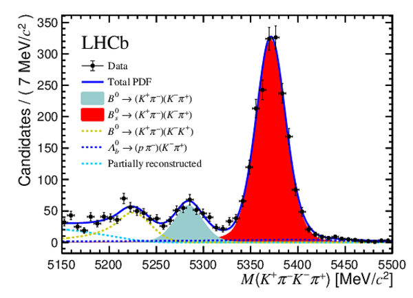
Aggregated four-body invariant-mass fit result of the 2011 and 2012 data. The solid red distribution corresponds to the $ B ^0_ s \rightarrow ( K ^+ \pi ^- )( K ^- \pi ^+ )$ decay, the solid cyan distribution to $ B ^0 \rightarrow ( K ^+ \pi ^- )( K ^- \pi ^+ )$ , the dotted dark blue line to $\Lambda ^0_ b \rightarrow ( p \pi ^- )( K ^- \pi ^+ )$ , the dotted yellow line to $ B ^0 \rightarrow ( K ^+ \pi ^- )( K ^- K ^+ )$ and the dotted cyan line represents the partially reconstructed background. The tiny combinatorial background contribution is not represented. The black points with error bars correspond to data to which the $ B ^0 \rightarrow \rho ^0 K ^{*0} $ contribution has been subtracted with negatively weighted simulation, and the overall fit is represented by the thick blue line.

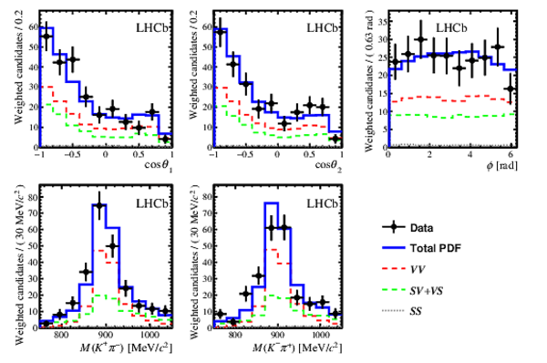
Projections of the amplitude fit results for the $ B ^0 \rightarrow K ^{*0} \overline{ K } {}^{*0} $ decay mode on the helicity angles (top row: $\cos \theta_1$ left, $\cos \theta_2$ centre and $\phi$ right) and on the two-body invariant masses (bottom row: $M( K ^+ \pi ^- )$ left and $M( K ^- \pi ^+ )$ centre). The contributing partial waves: $VV$ (dashed red), $VS$ (dashed green) and $SS$ (dotted grey) are shown with lines. The black points correspond to data and the overall fit is represented by the blue line.

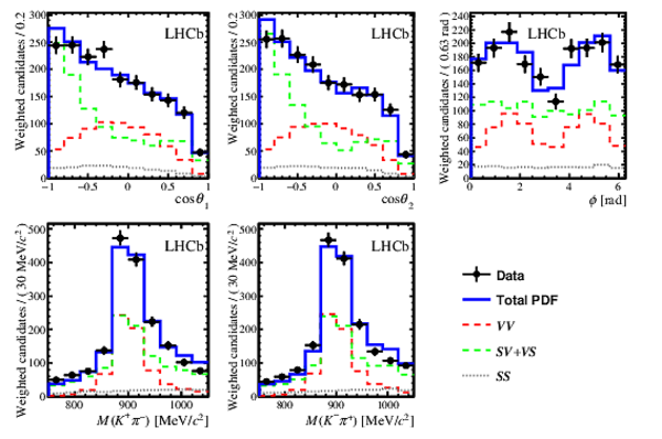
Projections of the amplitude fit results for the $ B ^0_ s \rightarrow K ^{*0} \overline{ K } {}^{*0} $ decay mode on the helicity angles (top row: $\cos \theta_1$ left, $\cos \theta_2$ centre and $\phi$ right) and on the two-body invariant masses (bottom row: $M( K ^+ \pi ^- )$ left and $M( K ^- \pi ^+ )$ centre). The contributing partial waves: $VV$ (dashed red), $VS$ (dashed green) and $SS$ (dotted grey) are shown with lines. The black points correspond to data and the overall fit is represented by the blue line.

Animated gif made out of all figures.

Parameters of the mass propagators employed in the amplitude analysis.

Amplitudes, $A_i$, and angle-mass functions, $g_i(m_1,m_2,\theta_1,\theta_2,\phi)$, of the differential decay rate of 5. In particular, $A_0$, $A_\parallel$ and $A_\perp$ are the longitudinal, parallel and transverse helicity amplitudes of the {P--wave} whereas $A_S^+$ and $A_S^-$ are the combinations of $ C P$ eigenstate amplitudes of the $SV$ and $VS$ states and $A_{SS}$ is the double {S--wave} amplitude. The table indicates the corresponding $ C P$ eigenvalue, $\eta_i$. The mass propagators, $\mathcal{M}_{0,1}(m)$, are discussed in the text.

Signal and background yields for the 2011 and 2012 data samples, obtained from the fit to the four-body mass spectrum of the selected candidates. Statistical and systematic uncertainties are reported, the latter are estimated as explained in Sect. ???.

Results of the amplitude analysis of $ B ^0 \rightarrow ( K ^+ \pi ^- )( K ^- \pi ^+ )$ and $ B ^0_ s \rightarrow ( K ^+ \pi ^- )( K ^- \pi ^+ )$ decays. The observables above the line are directly obtained from the maximum-likelihood fit whereas those below are obtained from the former, as explained in the text, with correlations accounted for in their estimated uncertainties. For each result, the first quoted uncertainty is statistical and the second systematic. The estimation of the latter is described in Sect. ???.

Alternative parameters of the LASS mass propagator used in the {S--wave} systematic uncertainty estimation.

Systematic uncertainties for the parameters of the amplitude-analysis fit of the $ B ^0_{( s )} \rightarrow ( K ^+ \pi ^- )( K ^- \pi ^+ )$ decay. The bias related to differences between data and simulation is included in the results shown in Table ???.

Systematic uncertainties for the derived observables of the amplitude-analysis fit of the $ B ^0_{( s )} \rightarrow ( K ^+ \pi ^- )( K ^- \pi ^+ )$ decay. The bias related to differences between data and simulation is included in the results shown in Table ???.

Systematic uncertainties in the factor $\kappa$ defined in 12 split in categories. The bias originated in differences between data and simulation is corrected for in the $\kappa$ results shown in Table ???.

Parameters used to determine $\mathcal{B} ( B ^0 \rightarrow K ^{*0} \overline{ K } {}^{*0} )/\mathcal{B} ( B ^0_ s \rightarrow K ^{*0} \overline{ K } {}^{*0} )$. When two uncertainties are quoted, the first is statistical and the second systematic. The value of $f_s/f_d$ is taken from Ref. [44].