Search for lepton-universality violation in $B^+\to K^+\ell^+\ell^-$ decays
[to restricted-access page]Information
LHCb-PAPER-2019-009
CERN-EP-2019-043
arXiv:1903.09252 [PDF]
(Submitted on 21 Mar 2019)
Phys. Rev. Lett. 122 (2019) 191801
Inspire 1726420
Tools
Abstract
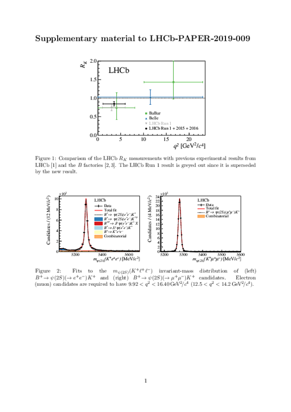
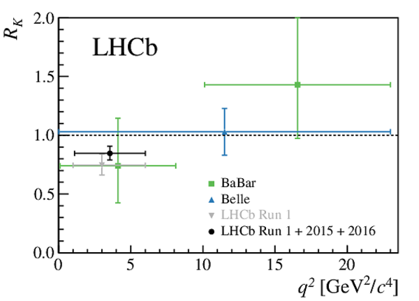
A measurement of the ratio of branching fractions of the decays $B^+\to K^+\mu^+\mu^-$ and $B^+\to K^+e^+e^-$ is presented. The proton-proton collision data used correspond to an integrated luminosity of $5.0 $fb$^{-1}$ recorded with the LHCb experiment at centre-of-mass energies of $7$, $8$ and $13 $TeV. For the dilepton mass-squared range $1.1 < q^2 < 6.0 $GeV$^2 /c^4$ the ratio of branching fractions is measured to be $R_K = {0.846 ^{+ 0.060}_{- 0.054} ^{+ 0.016}_{- 0.014}}$, where the first uncertainty is statistical and the second systematic. This is the most precise measurement of $R_K$ to date and is compatible with the Standard Model at the level of 2.5 standard deviations.
Figures and captions
|
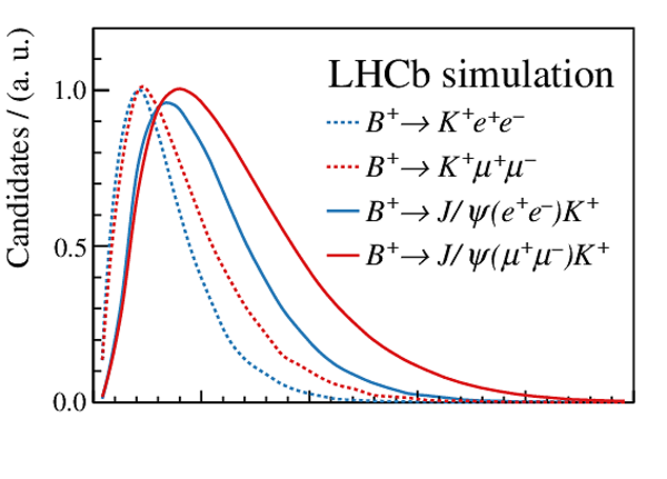
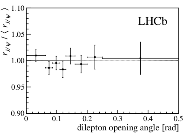
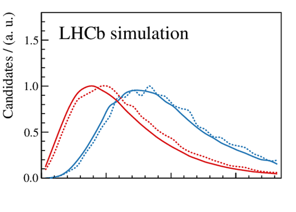
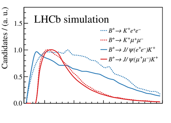
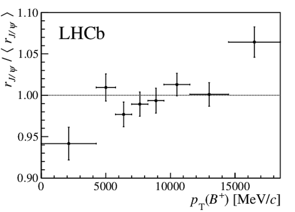
(Top) expected distributions of the opening angle between the two leptons, in the laboratory frame, for the four modes in the double ratio used to determine $ R_{ K }$ . (Bottom) the single ratio $ r_{ { J \mskip -3mu/\mskip -2mu\psi \mskip 2mu} }$ relative to its average value $\left< r_{ { J \mskip -3mu/\mskip -2mu\psi \mskip 2mu} } \right>$ as a function of the opening angle. |
Fig1a.pdf [15 KiB] HiDef png [332 KiB] Thumbnail [200 KiB] *.C file |
|
|
Fig1b.pdf [14 KiB] HiDef png [89 KiB] Thumbnail [46 KiB] *.C file |
|
|
|
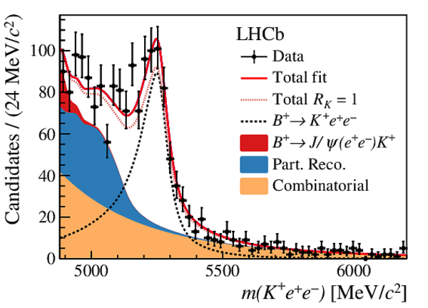
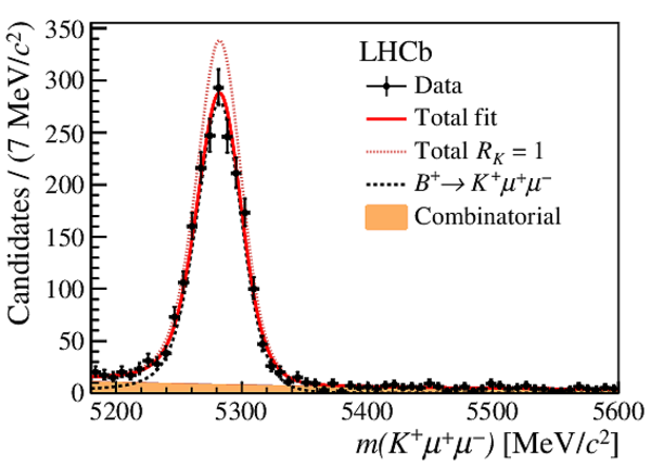
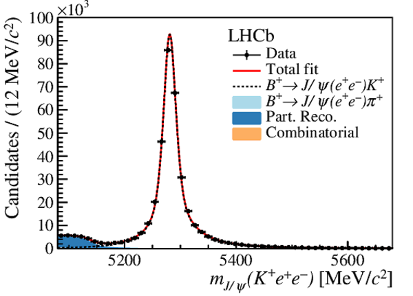
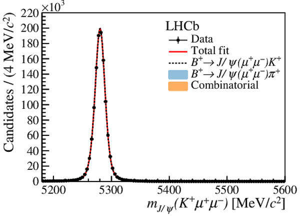
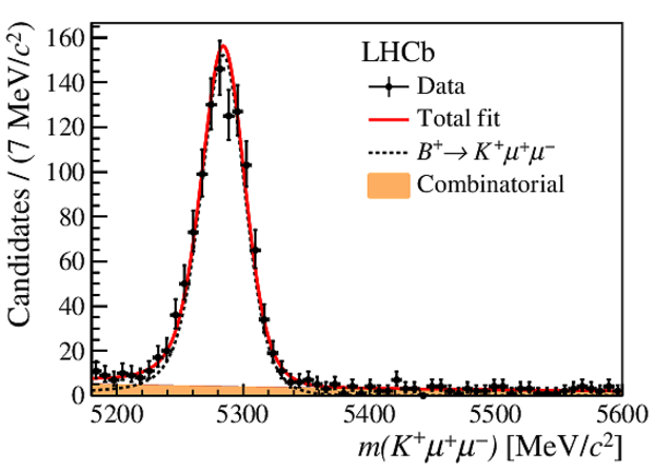
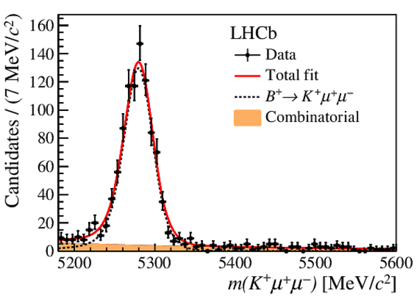
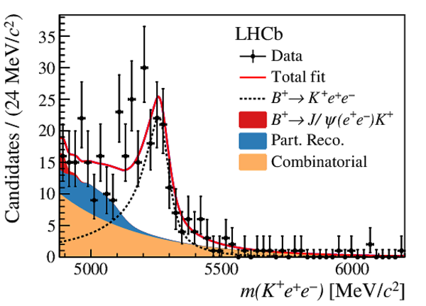
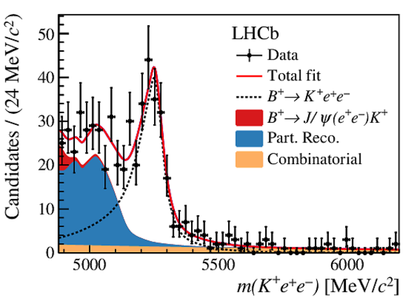
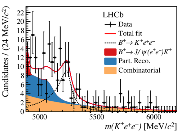
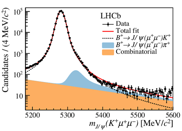
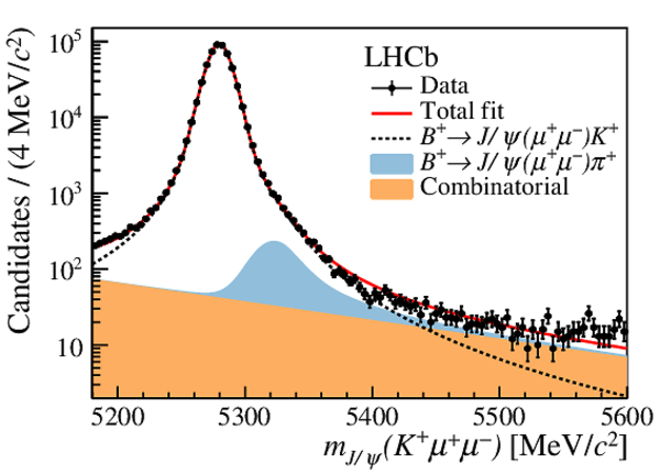
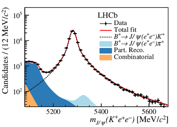
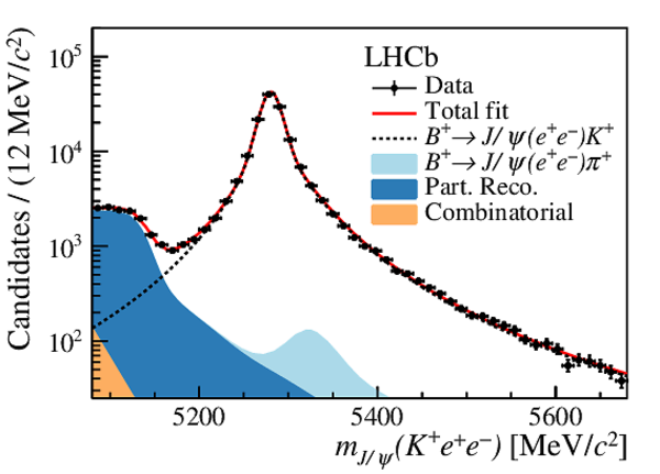
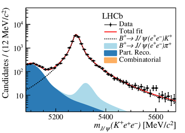
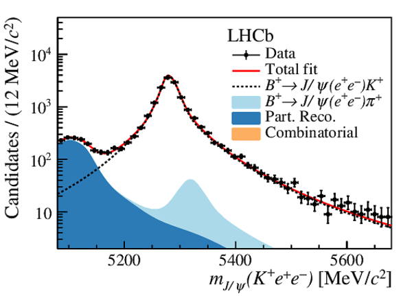
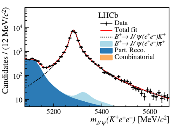
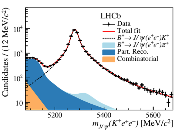
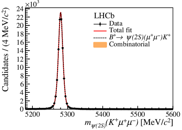
Fits to the $ m_{( { J \mskip -3mu/\mskip -2mu\psi \mskip 2mu} )}{( K ^+ \ell^+ \ell^- )}$ invariant mass distribution for (left) electron and (right) muon candidates for (top) nonresonant and (bottom) resonant decays. For the electron (muon) nonresonant plots, the red-dotted line shows the distribution that would be expected from the observed number of $ B ^+ \rightarrow K ^+ \mu ^+\mu ^- $ ( $ B ^+ \rightarrow K ^+ e ^+ e ^- $ ) decays and $ R_{ K } =1$. |
Fig2a.pdf [27 KiB] HiDef png [361 KiB] Thumbnail [264 KiB] *.C file |
|
|
Fig2b.pdf [27 KiB] HiDef png [277 KiB] Thumbnail [209 KiB] *.C file |
|
|
|
Fig2c.pdf [22 KiB] HiDef png [234 KiB] Thumbnail [201 KiB] *.C file |
|
|
|
Fig2d.pdf [36 KiB] HiDef png [224 KiB] Thumbnail [202 KiB] *.C file |
|
|
|
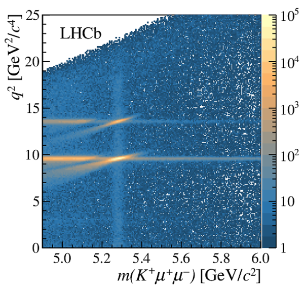
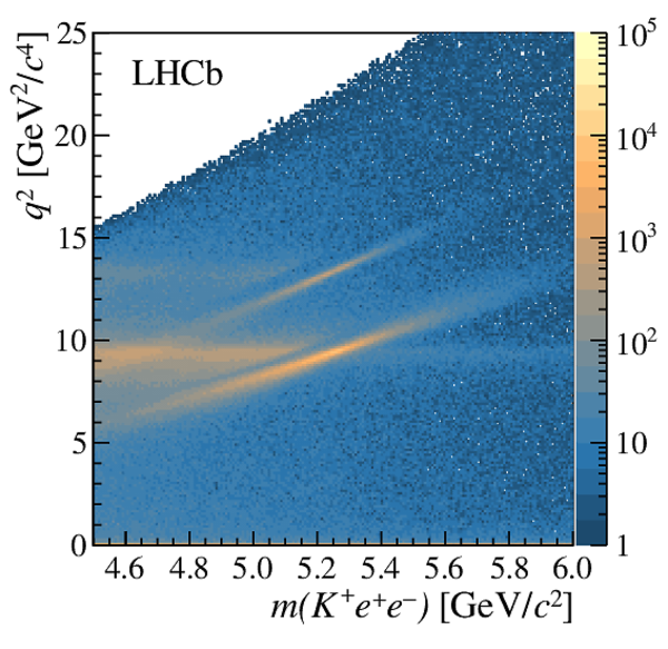
Two-dimensional distributions of $[ m({ K ^+ \ell^+ \ell^- }) , q^2 ]$ for (left) muon and (right) electron candidates after the application of the pre-selection and trigger requirements but not the multivariate selection. |
FigS1a.pdf [169 KiB] HiDef png [3 MiB] Thumbnail [1 MiB] *.C file |
|
|
FigS1b.pdf [163 KiB] HiDef png [2 MiB] Thumbnail [1 MiB] *.C file |
|
|
|
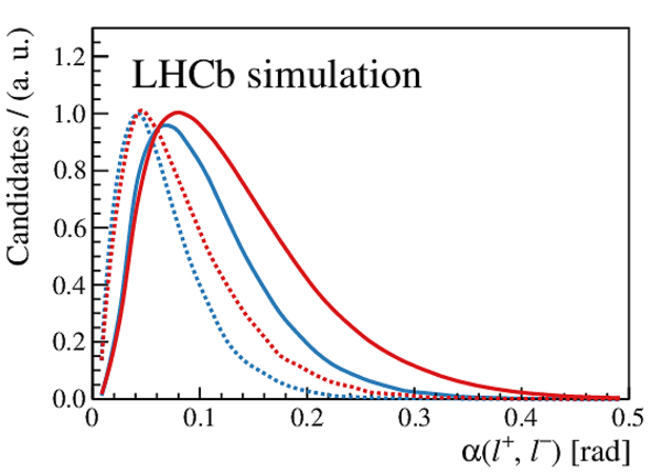
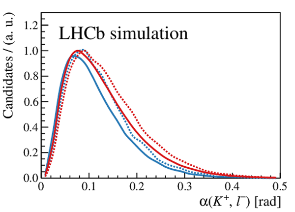
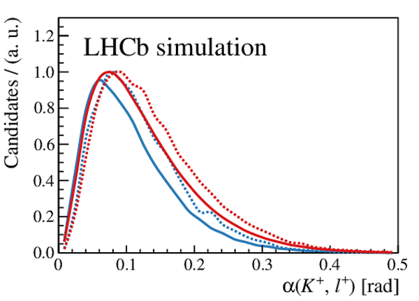
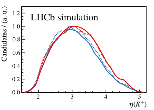
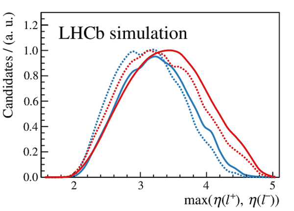
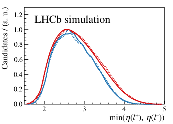
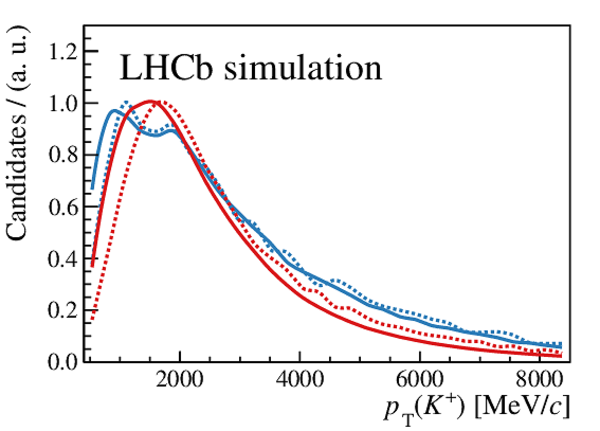
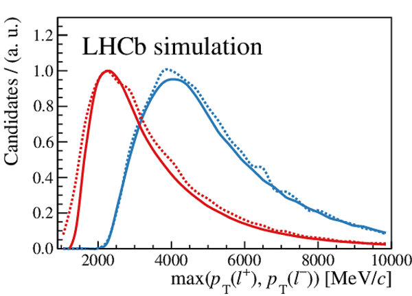
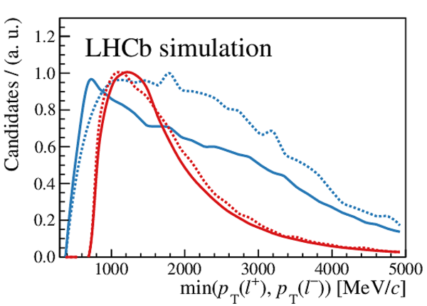
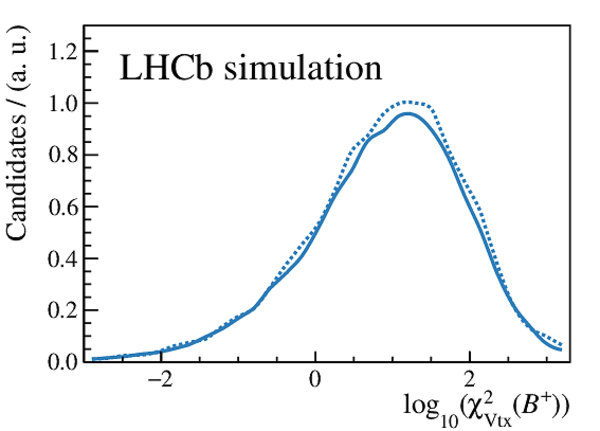
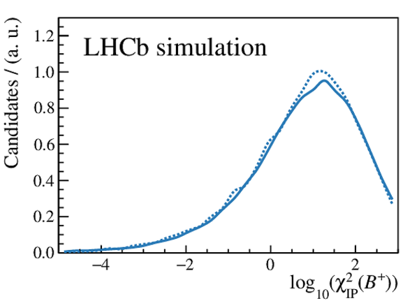
Distributions of various reconstructed properties for simulated decays. The first row shows the angle between the two leptons, or one lepton and the kaon. The second row shows the rapidity distributions, and the third row the transverse momentum distributions of all the final-state particles. The bottom left plot shows the distribution for the quality of the $ B ^+ $ vertex fit and the bottom right plot shows the $\chi^2_{\text{IP}} ( B ^+ )$ variable, which quantifies the significance of the $ B ^+ $ impact parameter. |
FigS2a.pdf [15 KiB] HiDef png [318 KiB] Thumbnail [194 KiB] *.C file |
|
|
FigS2b.pdf [15 KiB] HiDef png [308 KiB] Thumbnail [186 KiB] *.C file |
|
|
|
FigS2c.pdf [15 KiB] HiDef png [307 KiB] Thumbnail [188 KiB] *.C file |
|
|
|
FigS2d.pdf [15 KiB] HiDef png [258 KiB] Thumbnail [157 KiB] *.C file |
|
|
|
FigS2e.pdf [15 KiB] HiDef png [309 KiB] Thumbnail [190 KiB] *.C file |
|
|
|
FigS2f.pdf [15 KiB] HiDef png [270 KiB] Thumbnail [165 KiB] *.C file |
|
|
|
FigS2g.pdf [15 KiB] HiDef png [310 KiB] Thumbnail [196 KiB] *.C file |
|
|
|
FigS2h.pdf [15 KiB] HiDef png [334 KiB] Thumbnail [217 KiB] *.C file |
|
|
|
FigS2i.pdf [16 KiB] HiDef png [341 KiB] Thumbnail [222 KiB] *.C file |
|
|
|
FigS2j.pdf [14 KiB] HiDef png [194 KiB] Thumbnail [136 KiB] *.C file |
|
|
|
FigS2k.pdf [14 KiB] HiDef png [179 KiB] Thumbnail [129 KiB] *.C file |
|
|
|
FigS2l.pdf [12 KiB] HiDef png [94 KiB] Thumbnail [92 KiB] *.C file |

|
|
|
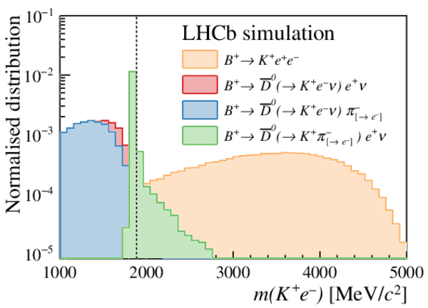
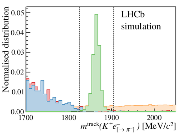
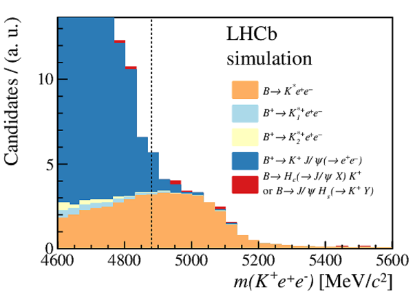
Simulated $K^+e^-$ mass distributions for signal and various cascade background samples. The distributions are all normalised to unity. (Left) the bremsstrahlung correction to the momentum of the electron is taken into account, resulting in a tail to the right. (Right) the mass is computed only from the track information ($m^{\mathrm{track}}$). The notation $\pi_{[\rightarrow e]}$ ($e_{[\rightarrow \pi]}$) is used to denote an electron (pion) that is misidentified as a pion (electron). |
FigS3a.pdf [15 KiB] HiDef png [252 KiB] Thumbnail [197 KiB] *.C file |
|
|
FigS3b.pdf [14 KiB] HiDef png [208 KiB] Thumbnail [172 KiB] *.C file |
|
|
|
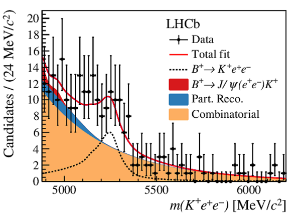
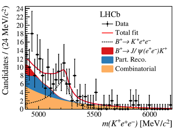
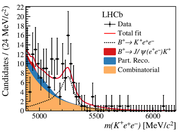
Fit to the $ m({ K ^+ \ell^+ \ell^- })$ invariant-mass distribution of nonresonant candidates in the (left) 7 and 8 $\text{ Te V}$ and (right) 13 $\text{ Te V}$ data samples. The top row shows the fit to the muon modes and the subsequent rows the fits to the electron modes triggered by (second row) one of the electrons, (third row) the kaon and (last row) by other particles in the event. |
FigS4a.pdf [26 KiB] HiDef png [245 KiB] Thumbnail [195 KiB] *.C file |
|
|
FigS4b.pdf [26 KiB] HiDef png [239 KiB] Thumbnail [194 KiB] *.C file |
|
|
|
FigS4c.pdf [21 KiB] HiDef png [291 KiB] Thumbnail [231 KiB] *.C file |
|
|
|
FigS4d.pdf [26 KiB] HiDef png [296 KiB] Thumbnail [229 KiB] *.C file |
|
|
|
FigS4e.pdf [21 KiB] HiDef png [332 KiB] Thumbnail [255 KiB] *.C file |
|
|
|
FigS4f.pdf [21 KiB] HiDef png [302 KiB] Thumbnail [241 KiB] *.C file |
|
|
|
FigS4g.pdf [21 KiB] HiDef png [293 KiB] Thumbnail [236 KiB] *.C file |
|
|
|
FigS4h.pdf [21 KiB] HiDef png [313 KiB] Thumbnail [244 KiB] *.C file |
|
|
|
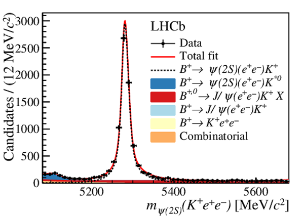
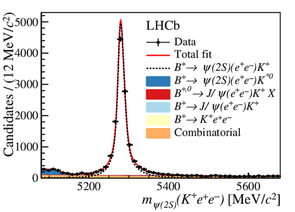
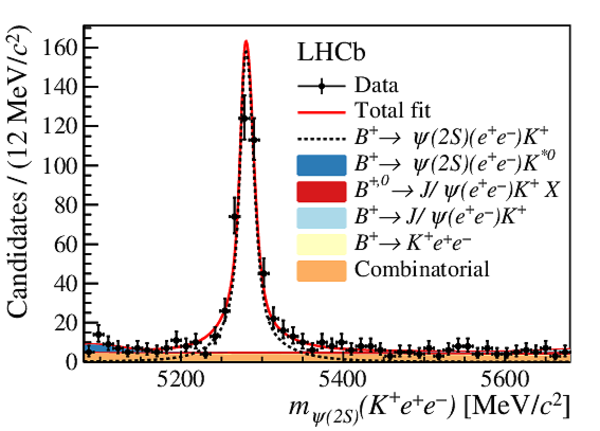
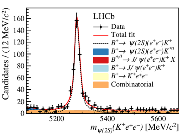
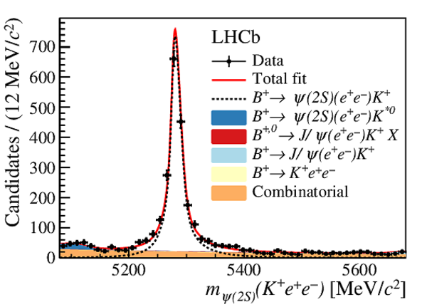
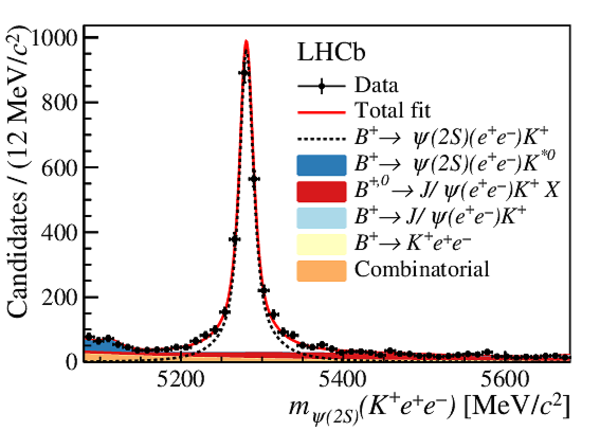
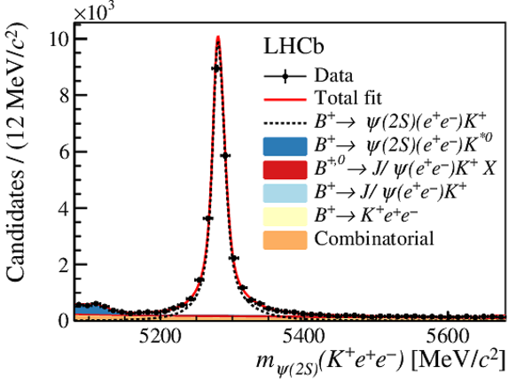
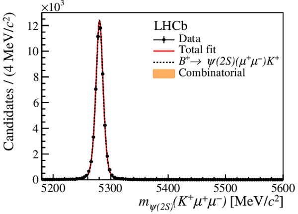
Fit to the $ m_{ { J \mskip -3mu/\mskip -2mu\psi \mskip 2mu} }{( K ^+ \ell^+ \ell^- )}$ invariant-mass distribution of resonant candidates in the (left) 7 and 8 $\text{ Te V}$ and (right) 13 $\text{ Te V}$ data samples. The top row shows the fit to the muon modes and the subsequent rows the fits to the electron modes triggered by (second row) one of the electrons, (third row) the kaon and (last row) by other particles in the event. Some large pulls are observed but have a negligible impact on the yields extracted. |
FigS5a.pdf [37 KiB] HiDef png [295 KiB] Thumbnail [241 KiB] *.C file |
|
|
FigS5b.pdf [37 KiB] HiDef png [295 KiB] Thumbnail [238 KiB] *.C file |
|
|
|
FigS5c.pdf [21 KiB] HiDef png [238 KiB] Thumbnail [200 KiB] *.C file |
|
|
|
FigS5d.pdf [21 KiB] HiDef png [241 KiB] Thumbnail [202 KiB] *.C file |
|
|
|
FigS5e.pdf [21 KiB] HiDef png [246 KiB] Thumbnail [210 KiB] *.C file |
|
|
|
FigS5f.pdf [21 KiB] HiDef png [246 KiB] Thumbnail [209 KiB] *.C file |
|
|
|
FigS5g.pdf [21 KiB] HiDef png [243 KiB] Thumbnail [206 KiB] *.C file |
|
|
|
FigS5h.pdf [21 KiB] HiDef png [246 KiB] Thumbnail [206 KiB] *.C file |
|
|
|
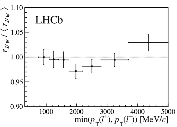
(Top) distributions of the spectra of (left) the $ B ^+ $ transverse momentum and (right) the minimum $ p_{\mathrm{T}}$ of the leptons. (Bottom) the single ratio $ r_{ { J \mskip -3mu/\mskip -2mu\psi \mskip 2mu} }$ relative to its average value $\left< r_{ { J \mskip -3mu/\mskip -2mu\psi \mskip 2mu} } \right>$ as a function of these variables. |
FigS6a.pdf [15 KiB] HiDef png [246 KiB] Thumbnail [146 KiB] *.C file |
|
|
FigS6b.pdf [16 KiB] HiDef png [278 KiB] Thumbnail [178 KiB] *.C file |
|
|
|
FigS6c.pdf [14 KiB] HiDef png [84 KiB] Thumbnail [43 KiB] *.C file |
|
|
|
FigS6d.pdf [14 KiB] HiDef png [95 KiB] Thumbnail [48 KiB] *.C file |
|
|
|
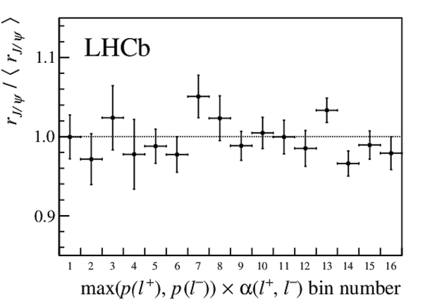
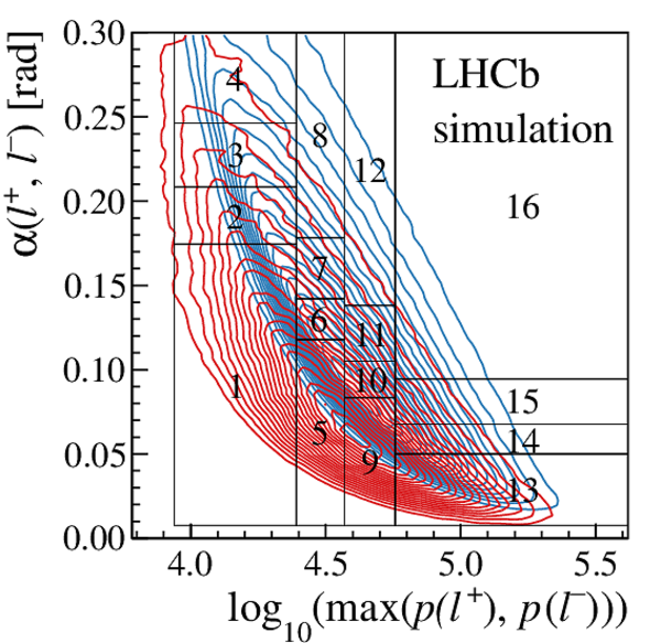
(Left) the value of $ r_{ { J \mskip -3mu/\mskip -2mu\psi \mskip 2mu} }$ , relative to the average value of $ r_{ { J \mskip -3mu/\mskip -2mu\psi \mskip 2mu} }$ , measured in two-dimensional bins of the maximum lepton momentum ($p(l)$) and the opening angle between the two leptons ($\alpha(l^+,l^-)$). (Right) the bin definition in this two-dimensional space together with the distribution for $ B ^+ \rightarrow K ^+ e ^+ e ^- $ ( $ B ^+ \rightarrow { J \mskip -3mu/\mskip -2mu\psi \mskip 2mu} (\rightarrow e ^+ e ^- ) K ^+ $ ) decays depicted as red (blue) contours. |
FigS7a.pdf [14 KiB] HiDef png [91 KiB] Thumbnail [48 KiB] *.C file |
|
|
FigS7b.pdf [63 KiB] HiDef png [1 MiB] Thumbnail [599 KiB] *.C file |
|
|
|
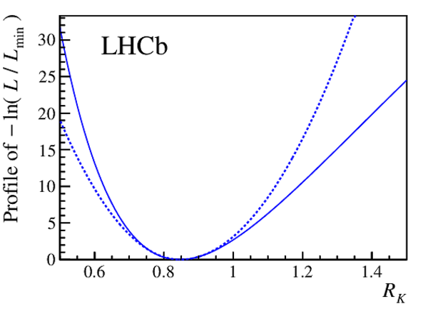
Likelihood function from the fit to the data profiled as a function of $ R_{ K }$ (solid line). The blue dashed line depicts the expected shape of the likelihood profile if the uncertainties were Gaussian. |
FigS8.pdf [15 KiB] HiDef png [138 KiB] Thumbnail [107 KiB] *.C file |
|
|
Animated gif made out of all figures. |
PAPER-2019-009.gif Thumbnail |

|
Tables and captions
|
Resonant and nonresonant mode $ q^2 $ and $ m({ K ^+ \ell^+ \ell^- })$ ranges. The variables $ m({ K ^+ \ell^+ \ell^- })$ and $ m_{ { J \mskip -3mu/\mskip -2mu\psi \mskip 2mu} }{( K ^+ \ell^+ \ell^- )}$ are used for nonresonant and resonant decays, respectively. |
Table_1.pdf [62 KiB] HiDef png [56 KiB] Thumbnail [26 KiB] tex code |

|
|
Total yields of the decay modes $ B ^+ \rightarrow K ^+ e ^+ e ^- $ , $ B ^+ \rightarrow K ^+ \mu ^+\mu ^- $ , $ B ^+ \rightarrow { J \mskip -3mu/\mskip -2mu\psi \mskip 2mu} (\rightarrow e ^+ e ^- ) K ^+ $ and $ B ^+ \rightarrow { J \mskip -3mu/\mskip -2mu\psi \mskip 2mu} (\rightarrow \mu ^+\mu ^- ) K ^+ $ obtained from the fits to the data. |
Table_2.pdf [60 KiB] HiDef png [60 KiB] Thumbnail [29 KiB] tex code |

|
Supplementary Material [file]

![HiDef png [332 KiB]](Directory_LHCb-PAPER-2019-009/hidef_Fig1a.png)
![HiDef png [89 KiB]](Directory_LHCb-PAPER-2019-009/hidef_Fig1b.png)
![HiDef png [361 KiB]](Directory_LHCb-PAPER-2019-009/hidef_Fig2a.png)
![HiDef png [277 KiB]](Directory_LHCb-PAPER-2019-009/hidef_Fig2b.png)
![HiDef png [234 KiB]](Directory_LHCb-PAPER-2019-009/hidef_Fig2c.png)
![HiDef png [224 KiB]](Directory_LHCb-PAPER-2019-009/hidef_Fig2d.png)
![HiDef png [3 MiB]](Directory_LHCb-PAPER-2019-009/hidef_FigS1a.png)
![HiDef png [2 MiB]](Directory_LHCb-PAPER-2019-009/hidef_FigS1b.png)
![HiDef png [318 KiB]](Directory_LHCb-PAPER-2019-009/hidef_FigS2a.png)
![HiDef png [308 KiB]](Directory_LHCb-PAPER-2019-009/hidef_FigS2b.png)
![HiDef png [307 KiB]](Directory_LHCb-PAPER-2019-009/hidef_FigS2c.png)
![HiDef png [258 KiB]](Directory_LHCb-PAPER-2019-009/hidef_FigS2d.png)
![HiDef png [309 KiB]](Directory_LHCb-PAPER-2019-009/hidef_FigS2e.png)
![HiDef png [270 KiB]](Directory_LHCb-PAPER-2019-009/hidef_FigS2f.png)
![HiDef png [310 KiB]](Directory_LHCb-PAPER-2019-009/hidef_FigS2g.png)
![HiDef png [334 KiB]](Directory_LHCb-PAPER-2019-009/hidef_FigS2h.png)
![HiDef png [341 KiB]](Directory_LHCb-PAPER-2019-009/hidef_FigS2i.png)
![HiDef png [194 KiB]](Directory_LHCb-PAPER-2019-009/hidef_FigS2j.png)
![HiDef png [179 KiB]](Directory_LHCb-PAPER-2019-009/hidef_FigS2k.png)
![HiDef png [94 KiB]](Directory_LHCb-PAPER-2019-009/hidef_FigS2l.png)
![HiDef png [252 KiB]](Directory_LHCb-PAPER-2019-009/hidef_FigS3a.png)
![HiDef png [208 KiB]](Directory_LHCb-PAPER-2019-009/hidef_FigS3b.png)
![HiDef png [245 KiB]](Directory_LHCb-PAPER-2019-009/hidef_FigS4a.png)
![HiDef png [239 KiB]](Directory_LHCb-PAPER-2019-009/hidef_FigS4b.png)
![HiDef png [291 KiB]](Directory_LHCb-PAPER-2019-009/hidef_FigS4c.png)
![HiDef png [296 KiB]](Directory_LHCb-PAPER-2019-009/hidef_FigS4d.png)
![HiDef png [332 KiB]](Directory_LHCb-PAPER-2019-009/hidef_FigS4e.png)
![HiDef png [302 KiB]](Directory_LHCb-PAPER-2019-009/hidef_FigS4f.png)
![HiDef png [293 KiB]](Directory_LHCb-PAPER-2019-009/hidef_FigS4g.png)
![HiDef png [313 KiB]](Directory_LHCb-PAPER-2019-009/hidef_FigS4h.png)
![HiDef png [295 KiB]](Directory_LHCb-PAPER-2019-009/hidef_FigS5a.png)
![HiDef png [295 KiB]](Directory_LHCb-PAPER-2019-009/hidef_FigS5b.png)
![HiDef png [238 KiB]](Directory_LHCb-PAPER-2019-009/hidef_FigS5c.png)
![HiDef png [241 KiB]](Directory_LHCb-PAPER-2019-009/hidef_FigS5d.png)
![HiDef png [246 KiB]](Directory_LHCb-PAPER-2019-009/hidef_FigS5e.png)
![HiDef png [246 KiB]](Directory_LHCb-PAPER-2019-009/hidef_FigS5f.png)
![HiDef png [243 KiB]](Directory_LHCb-PAPER-2019-009/hidef_FigS5g.png)
![HiDef png [246 KiB]](Directory_LHCb-PAPER-2019-009/hidef_FigS5h.png)
![HiDef png [246 KiB]](Directory_LHCb-PAPER-2019-009/hidef_FigS6a.png)
![HiDef png [278 KiB]](Directory_LHCb-PAPER-2019-009/hidef_FigS6b.png)
![HiDef png [84 KiB]](Directory_LHCb-PAPER-2019-009/hidef_FigS6c.png)
![HiDef png [95 KiB]](Directory_LHCb-PAPER-2019-009/hidef_FigS6d.png)
![HiDef png [91 KiB]](Directory_LHCb-PAPER-2019-009/hidef_FigS7a.png)
![HiDef png [1 MiB]](Directory_LHCb-PAPER-2019-009/hidef_FigS7b.png)
![HiDef png [138 KiB]](Directory_LHCb-PAPER-2019-009/hidef_FigS8.png)
![HiDef png [56 KiB]](Directory_LHCb-PAPER-2019-009/hidef_Table_1.png)
![HiDef png [60 KiB]](Directory_LHCb-PAPER-2019-009/hidef_Table_2.png)
![HiDef png [136 KiB]](Directory_LHCb-PAPER-2019-009/supplementary/hidef_13LogVtxCHI2Trig0.png)
![HiDef png [167 KiB]](Directory_LHCb-PAPER-2019-009/supplementary/hidef_1B_plus_PTTrig0_ee.png)
![HiDef png [158 KiB]](Directory_LHCb-PAPER-2019-009/supplementary/hidef_1B_plus_PTTrig0_mumu.png)
![HiDef png [158 KiB]](Directory_LHCb-PAPER-2019-009/supplementary/hidef_2016data_slice2.png)
![HiDef png [179 KiB]](Directory_LHCb-PAPER-2019-009/supplementary/hidef_Mass_BkgComponents.png)
![HiDef png [116 KiB]](Directory_LHCb-PAPER-2019-009/supplementary/hidef_RK2019.png)
![HiDef png [199 KiB]](Directory_LHCb-PAPER-2019-009/supplementary/hidef_effIn_bias_2016.png)
![HiDef png [289 KiB]](Directory_LHCb-PAPER-2019-009/supplementary/hidef_plotKPsi2SeeDataFitTrig0Run1.png)
![HiDef png [285 KiB]](Directory_LHCb-PAPER-2019-009/supplementary/hidef_plotKPsi2SeeDataFitTrig0Run2.png)
![HiDef png [316 KiB]](Directory_LHCb-PAPER-2019-009/supplementary/hidef_plotKPsi2SeeDataFitTrig1Run1.png)
![HiDef png [310 KiB]](Directory_LHCb-PAPER-2019-009/supplementary/hidef_plotKPsi2SeeDataFitTrig1Run2.png)
![HiDef png [303 KiB]](Directory_LHCb-PAPER-2019-009/supplementary/hidef_plotKPsi2SeeDataFitTrig2Run1.png)
![HiDef png [299 KiB]](Directory_LHCb-PAPER-2019-009/supplementary/hidef_plotKPsi2SeeDataFitTrig2Run2.png)
![HiDef png [279 KiB]](Directory_LHCb-PAPER-2019-009/supplementary/hidef_plotKPsi2SeeDataFitTrigAllRunAll.png)
![HiDef png [193 KiB]](Directory_LHCb-PAPER-2019-009/supplementary/hidef_plotKPsi2SmumuDataFitRun1.png)
![HiDef png [191 KiB]](Directory_LHCb-PAPER-2019-009/supplementary/hidef_plotKPsi2SmumuDataFitRun2.png)
![HiDef png [207 KiB]](Directory_LHCb-PAPER-2019-009/supplementary/hidef_plotKPsi2SmumuDataFitRunAll.png)
Created on 20 April 2024.