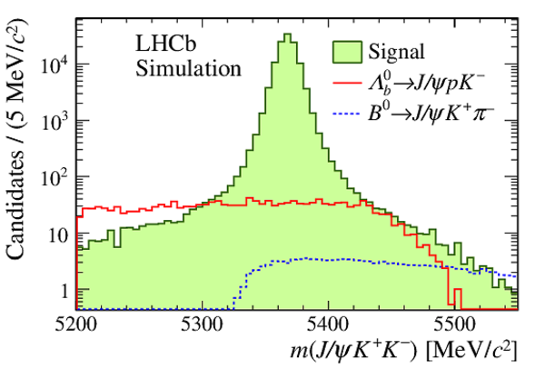
Distribution of the invariant mass of $ B ^0_ s $ candidates, selected from simulated $ B ^0_ s \rightarrow { J \mskip -3mu/\mskip -2mu\psi \mskip 2mu} K ^+ K ^- $ (green filled area), $\Lambda ^0_ b \rightarrow { J \mskip -3mu/\mskip -2mu\psi \mskip 2mu} p K ^- $ (solid red line) and $ B ^0 \rightarrow { J \mskip -3mu/\mskip -2mu\psi \mskip 2mu} K ^+ \pi ^- $ (dotted blue line) decays. The distributions are weighted to correct differences in the kinematics and the resonance content between simulation and data.

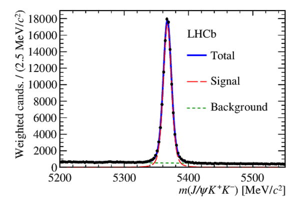
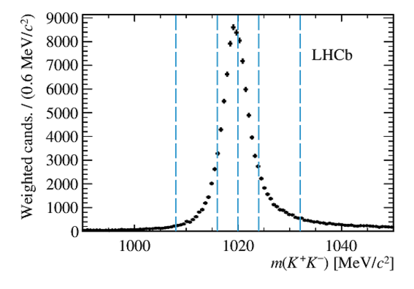
(a) Distribution of the invariant mass of selected $ B ^0_ s \rightarrow { J \mskip -3mu/\mskip -2mu\psi \mskip 2mu} K ^+ K ^- $ decays. The signal component is shown by the long-dashed red line, the background component by the dashed green line and the total fit function by the solid blue line. The background contribution due to $\Lambda ^0_ b \rightarrow { J \mskip -3mu/\mskip -2mu\psi \mskip 2mu} p K ^- $ decays is statistically subtracted. The contribution from $ B ^0 \rightarrow { J \mskip -3mu/\mskip -2mu\psi \mskip 2mu} K ^+ K ^- $decays is not shown separately due to its small size. (b) Distribution of $ K ^+ K ^- $ invariant mass from selected $ B ^0_ s \rightarrow { J \mskip -3mu/\mskip -2mu\psi \mskip 2mu} K ^+ K ^- $ decays. The background is subtracted using the $sPlot$ method. The dashed blue lines define the boundaries of the six $m(K^{+}K^{-})$ bins that are used in the analysis.

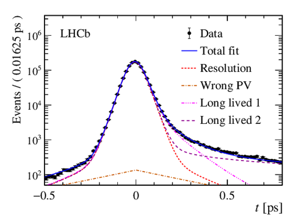
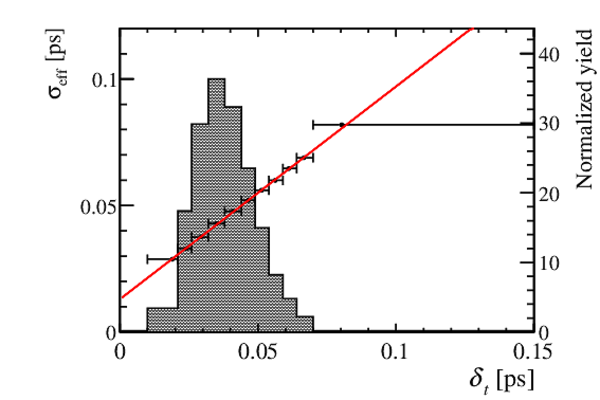
(a) Decay-time distribution of the prompt $ { J \mskip -3mu/\mskip -2mu\psi \mskip 2mu} K ^+ K ^- $ calibration sample with the result of an unbinned maximum-likelihood fit overlaid in blue. The overall triple-Gaussian resolution is represented by the dashed red line, while the two long-lived and the wrong-PV components are shown by the long-dashed-dotted and dashed-multiple-dotted brown and pink lines and the long-dashed purple line, respectively. (b) Variation of the effective single-Gaussian decay-time resolution, $\sigma_{\rm eff}$, as a function of the estimated per-candidate decay-time uncertainty, $\delta_t$, obtained from the prompt $ { J \mskip -3mu/\mskip -2mu\psi \mskip 2mu} K ^+ K ^- $ sample. The red line shows the result of a linear fit. The data points are positioned at the barycentre of each $\delta_t$ bin. The shaded histogram (see right $y$ axis) shows the distribution of $\delta_t$ in the background-subtracted $ B ^0_ s \rightarrow { J \mskip -3mu/\mskip -2mu\psi \mskip 2mu} K ^+ K ^- $ sample.

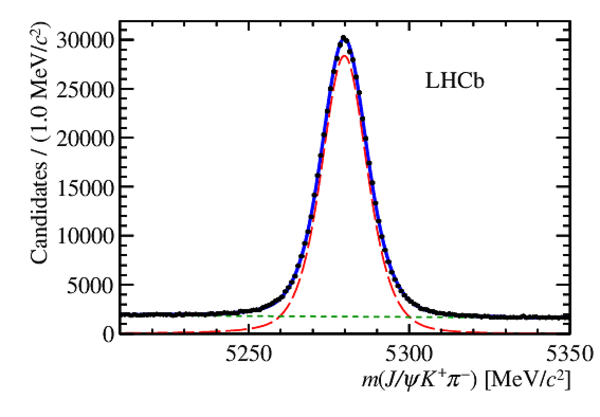
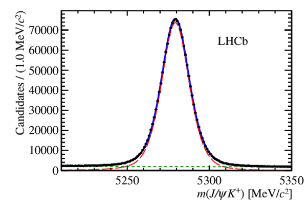
Distribution of the invariant mass of selected (a) $ B ^0 \rightarrow { J \mskip -3mu/\mskip -2mu\psi \mskip 2mu} K^+ \pi^-$ and (b) $B^+ \rightarrow { J \mskip -3mu/\mskip -2mu\psi \mskip 2mu} K^+$ decays used for the calibration and validation of the decay-time efficiency. The signal component is shown by the long-dashed red line, the background component by the dashed green line and the total fit function by the solid blue line.

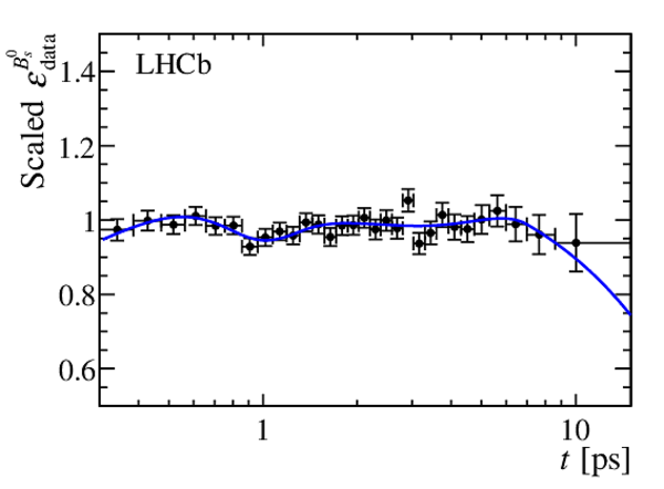
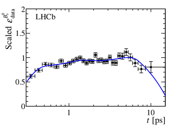
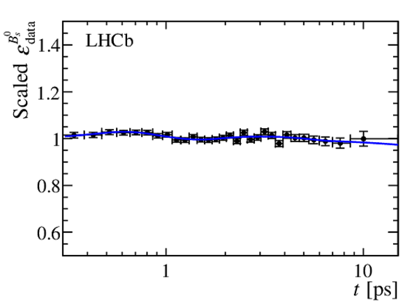
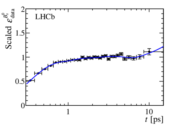
Decay-time efficiency for the (a) 2015 unbiased, (b) 2015 biased, (c) 2016 unbiased and (d) 2016 biased $ B ^0_ s \rightarrow { J \mskip -3mu/\mskip -2mu\psi \mskip 2mu} \phi$ sample. The cubic-spline function described in the text is shown by the blue line. For comparison, the black points show the efficiency when computed using histograms for each of the input component efficiencies.

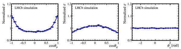
Normalised angular efficiency as a function of (a) $\cos\theta_K$, (b) $\cos\theta_\mu$ and (c) $\phi_h$, where in all cases the efficiency is integrated over the other two angles. The efficiency is evaluated using simulated $ B ^0_ s \rightarrow { J \mskip -3mu/\mskip -2mu\psi \mskip 2mu} \phi$ decays that have been weighted to match the kinematics and physics of $ B ^0_ s \rightarrow { J \mskip -3mu/\mskip -2mu\psi \mskip 2mu} K ^+ K ^- $ decays in data, as described in the text. The points are obtained by dividing the angular distribution in the simulated sample by the distribution expected without any efficiency effect and the curves represent an even fourth-order polynomial parameterisation of each one-dimensional efficiency. The figure is for illustration only as the angular efficiency is accounted for by normalisation weights in the signal PDF.

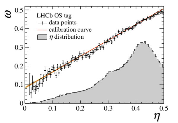
Calibration of the OS tagger using $ B ^+ \rightarrow { J \mskip -3mu/\mskip -2mu\psi \mskip 2mu} K ^+ $ decays. The black points show the average measured mistag probability, $\omega$, in bins of predicted mistag, $\eta$, the red line shows the calibration as described in the text and the yellow area the calibration uncertainty within one standard deviation. The shaded histogram shows the distribution, with arbitrary normalisation, of $\eta$ in the background subtracted $ B ^0_ s \rightarrow { J \mskip -3mu/\mskip -2mu\psi \mskip 2mu} \phi$ sample, summing over candidates tagged as $ B ^0_ s $ or $\overline{ B }{} {}^0_ s $.

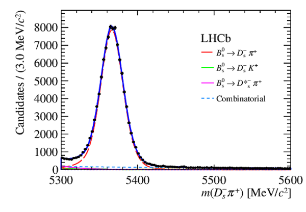
Distribution of the invariant mass of selected $ B ^0_ s \rightarrow D ^-_ s \pi^+$ candidates (black points). The total fit function is shown as the solid blue line. The signal component is shown by the red long-dashed line, the combinatorial background by the light-blue short-dashed line and other small background components are also shown as specified in the legend. Only the dominant backgrounds are shown.

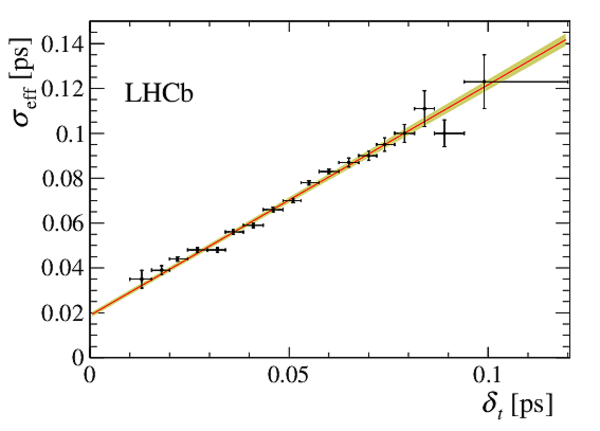
Variation of the effective single-Gaussian decay-time resolution, $\sigma_{\rm eff}$, as a function of the estimated per-event decay-time uncertainty, $\delta_t$, obtained from the prompt $ D ^-_ s \pi^+$ sample. The red line shows the result of a linear fit to the data and the yellow band its uncertainty within one standard deviation.

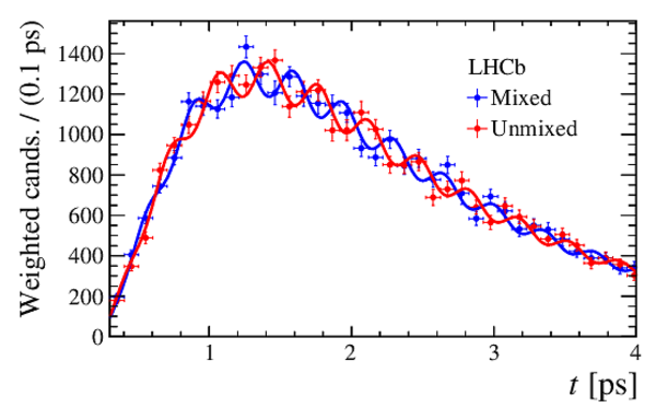
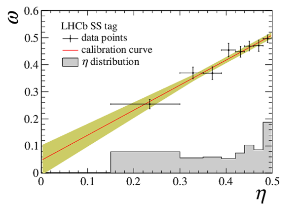
(a) Distribution of the decay time for $ B ^0_ s \rightarrow D ^-_ s \pi^+$ candidates tagged as mixed and unmixed with the projection of the fit result, which is described in the text. (b) Calibration of the SSK tagger using $ B ^0_ s \rightarrow D ^-_ s \pi^{+}$ decays. The black points show the average measured mistag probability, $\omega$, in bins of predicted mistag, $\eta$, the red line shows the calibration obtained from the fit described in the text, and the yellow area the calibration uncertainty within one standard deviation. The shaded histogram shows the distribution of $\eta$ in the background subtracted $ B ^0_ s \rightarrow { J \mskip -3mu/\mskip -2mu\psi \mskip 2mu} \phi$ sample.

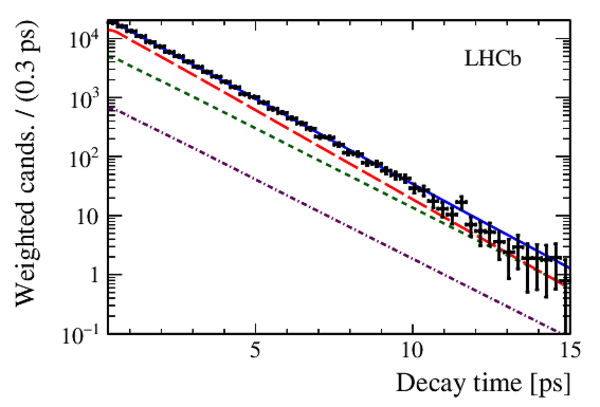
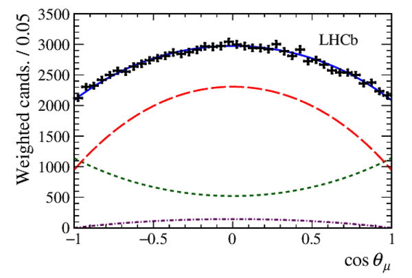
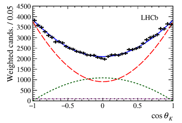
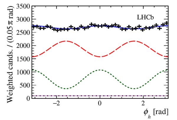
Decay-time and helicity-angle distributions for background subtracted $ B ^0_ s \rightarrow { J \mskip -3mu/\mskip -2mu\psi \mskip 2mu} K ^+ K ^- $ decays (data points) with the one-dimensional projections of the PDF at the maximum-likelihood point. The solid blue line shows the total signal contribution, which contains (long-dashed red) $ C P$ -even, (short-dashed green) $ C P$ -odd and (dotted-dashed purple) S-wave contributions. Data and fit projections for the different samples considered (data-taking year, trigger and tagging categories, $m(K^{+}K^{-})$ bins) are combined.

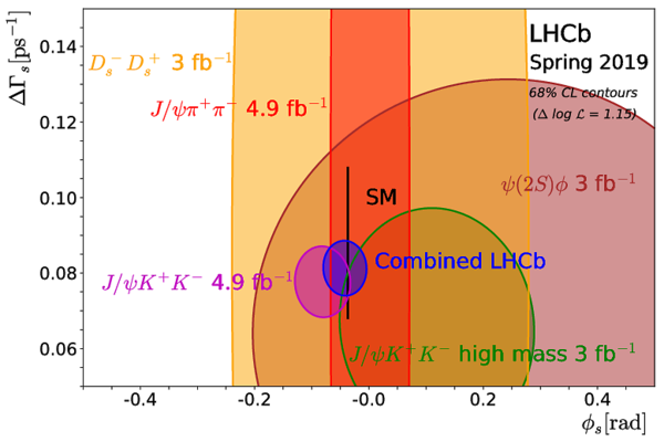
Regions of 68% confidence level in the $\phi_s$-$\Delta\Gamma_s$ plane for the individual LHCb measurements and a combined contour (in blue). The $ B ^0_ s \rightarrow { J \mskip -3mu/\mskip -2mu\psi \mskip 2mu} K ^+ K ^- $ (magenta) and $ B ^0_ s \rightarrow { J \mskip -3mu/\mskip -2mu\psi \mskip 2mu} \pi ^+ \pi ^- $ \cite{LHCb-PAPER-2019-003} (red) contours show the Run 1 and Run 2 combined numbers. The $\phi_s$ \cite{CKMfitter2015} and $\Delta\Gamma_{s}$ \cite{Artuso:2015swg} predictions are indicated by the thin black rectangle.

Animated gif made out of all figures.

Calibration parameters for the OS and SSK taggers. Where given, the first uncertainty is statistical and the second is systematic.

Overall tagging performance for $ B ^0_ s \rightarrow { J \mskip -3mu/\mskip -2mu\psi \mskip 2mu} K^{+}K^{-}$. The uncertainty on $\epsilon_{\rm tag}D^{2}$ is obtained by varying the tagging calibration parameters within their statistical and systematic uncertainties summed in quadrature.

Angular and time-dependent functions used in the fit to the data. Abbreviations used include $c_{K}=\cos\theta_K$, $s_{K}=\sin\theta_K$, $c_{l}=\cos\theta_l$, $s_{l}=\sin\theta_l$, $c_{\phi}=\cos\phi$ and $s_{\phi}=\sin\phi$.

Summary of the systematic uncertainties.

Correlation matrix including the statistical and systematic correlations between the parameters.

Correlation matrix for the results in Eq. \eqref{eq:comb1} taking into account correlated systematics between Run 1 and the 2015 and 2016 results.

Correlation matrix for the results in Eq. \eqref{eq:comb2} obtained taking into account correlated systematics between the considered analyses.

Values of the S-wave parameters in each $m(K^{+}K^{-})$ bin. The first uncertainty is statistical and the second systematic.