Amplitude analysis of the $B^+ \to \pi^+ \pi^+ \pi^-$ decay

Information

LHCb-PAPER-2019-017
CERN-EP-2019-157
arXiv:1909.05212 [PDF]

(Submitted on 11 Sep 2019)
Phys. Rev. D101 (2020) 012006
Inspire 1753654

Tools

Abstract

The results of an amplitude analysis of the charmless three-body decay $B^+ \rightarrow \pi^+\pi^+\pi^-$, in which $C P$-violation effects are taken into account, are reported. The analysis is based on a data sample corresponding to an integrated luminosity of $3 \text{fb}^{-1}$ of $pp$ collisions recorded with the LHCb detector. The most challenging aspect of the analysis is the description of the behaviour of the $\pi^+ \pi^-$ S-wave contribution, which is achieved by using three complementary approaches based on the isobar model, the K-matrix formalism, and a quasi-model-independent procedure. Additional resonant contributions for all three methods are described using a common isobar model, and include the $\rho(770)^0$, $\omega(782)$ and $\rho(1450)^0$ resonances in the $\pi^+\pi^-$ P-wave, the $f_2(1270)$ resonance in the $\pi^+\pi^-$ D-wave, and the $\rho_3(1690)^0$ resonance in the $\pi^+\pi^-$ F-wave. Significant $C P$-violation effects are observed in both S- and D-waves, as well as in the interference between the S- and P-waves. The results from all three approaches agree and provide new insight into the dynamics and the origin of $C P$-violation effects in $B^+ \rightarrow \pi^+\pi^+\pi^-$ decays.

Figures and captions

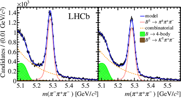
Invariant-mass fit model for (a) $ B ^- $ and (b) $ B ^+ $ candidates reconstructed in the $\pi ^\mp$ $\pi ^+$ $\pi ^-$ final state for the combined 2011 and 2012 data taking samples. Points with error bars represent the data while the components comprising the model are listed in the plot legend.	Fig1.pdf [49 KiB] HiDef png [356 KiB] Thumbnail [243 KiB] *.C file
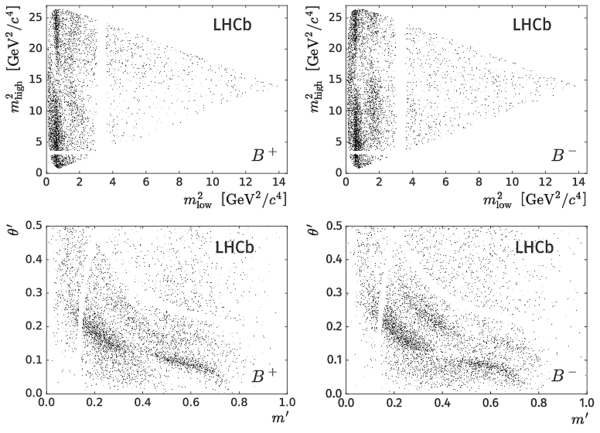
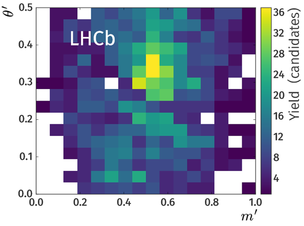
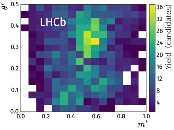
Conventional Dalitz-plot distributions for (a) $ B ^+ $ and (b) $ B ^- $ , and square Dalitz-plot (defined in Section 5.1.1) distributions for (c) $ B ^+ $ and (d) $ B ^- $ candidate decays to $\pi ^\pm \pi ^+ \pi ^- $. Depleted regions are due to the $\overline{ D } {}^0$ veto.	Fig2.pdf [555 KiB] HiDef png [546 KiB] Thumbnail [197 KiB] *.C file
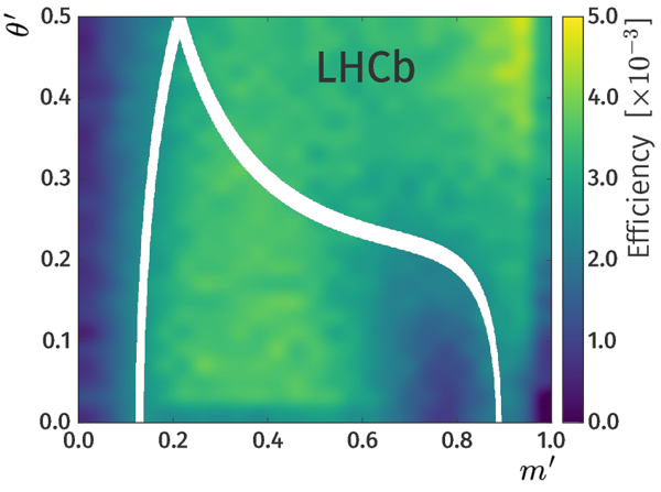
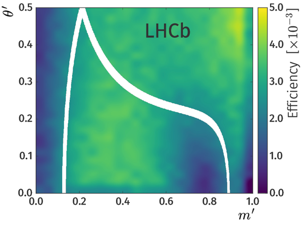
Square Dalitz-plot distributions for the (left) $ B ^+ $ and (right) $ B ^- $ signal efficiency models, smoothed using a two-dimensional cubic spline. Depleted regions are due to the $\overline{ D } {}^0$ veto.	Fig3a.pdf [250 KiB] HiDef png [2 MiB] Thumbnail [733 KiB] *.C file
	Fig3b.pdf [246 KiB] HiDef png [2 MiB] Thumbnail [733 KiB] *.C file
Square Dalitz-plot distributions for the (left) $ B ^+ $ and (right) $ B ^- $ combinatorial background models, scaled to represent their respective yields in the signal region.	Fig4a.pdf [56 KiB] HiDef png [194 KiB] Thumbnail [123 KiB] *.C file
	Fig4b.pdf [56 KiB] HiDef png [194 KiB] Thumbnail [124 KiB] *.C file
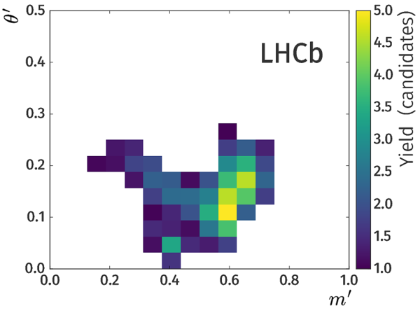
Square Dalitz-plot distribution for the misidentified $ B ^+ \rightarrow K ^+ \pi ^+ \pi ^- $ background model, scaled to represent its yield in the signal region.	Fig5.pdf [53 KiB] HiDef png [152 KiB] Thumbnail [105 KiB] *.C file
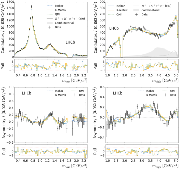
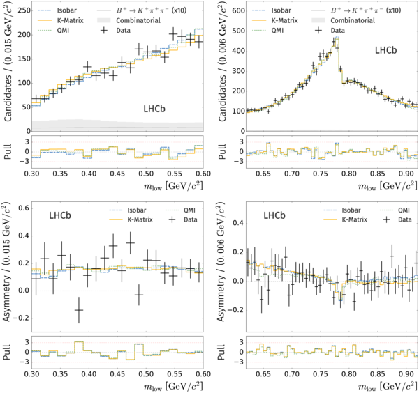
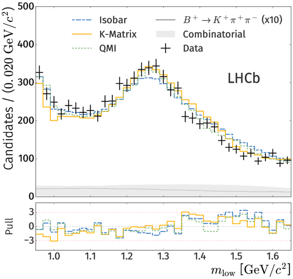
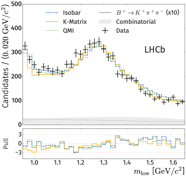
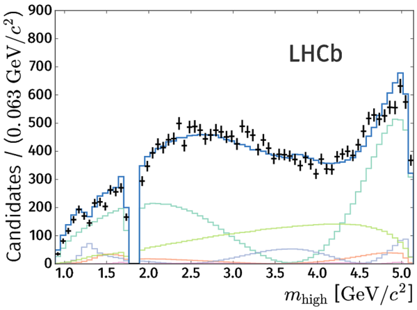
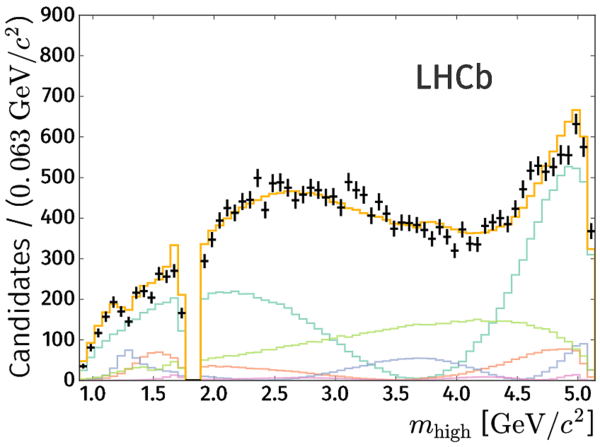
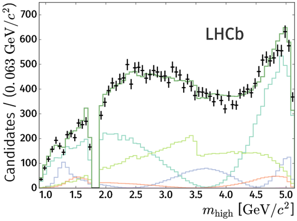
Fit projections of each model (a) in the low $m_{\rm low}$ region and (b) in the full range of $m_{\rm high}$, with the corresponding asymmetries shown beneath in (c) and (d). The normalised residual or pull distribution, defined as the difference between the bin value less the fit value over the uncertainty on the number of events in that bin, is shown below each fit projection.	Fig6.pdf [81 KiB] Thumbnail [418 KiB] *.C file
Fit projections of each model on $m_{\rm low}$ (a) in the region below the $\rho(770)^0$ resonance and (b) in the $\rho(770)^0$ region, with the corresponding asymmetries shown beneath in (c) and (d). The pull distribution is shown below each fit projection.	Fig7.pdf [60 KiB] Thumbnail [342 KiB] *.C file
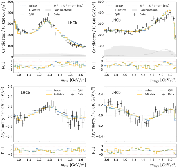
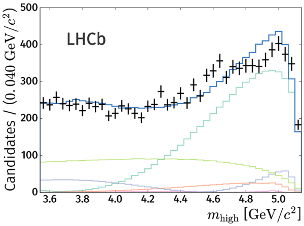
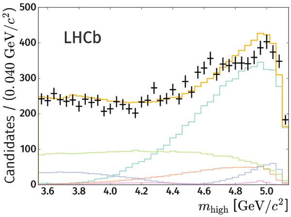
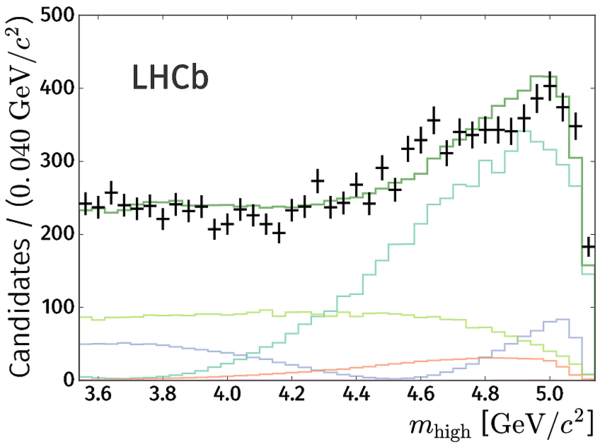
Fit projections of each model on $m_{\rm low}$ (a) in the region around the $f_2(1270)$ resonance and (b) in the high $m_{\rm high}$ region, with the corresponding asymmetries shown beneath in (c) and (d). The pull distribution is shown below each fit projection.	Fig8.pdf [61 KiB] Thumbnail [357 KiB] *.C file
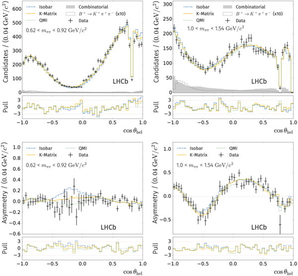
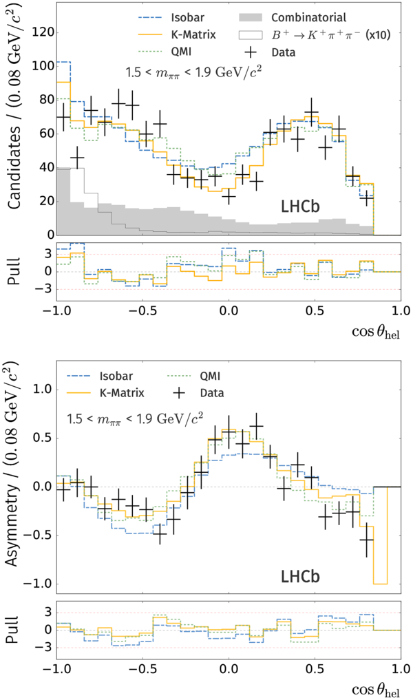
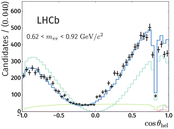
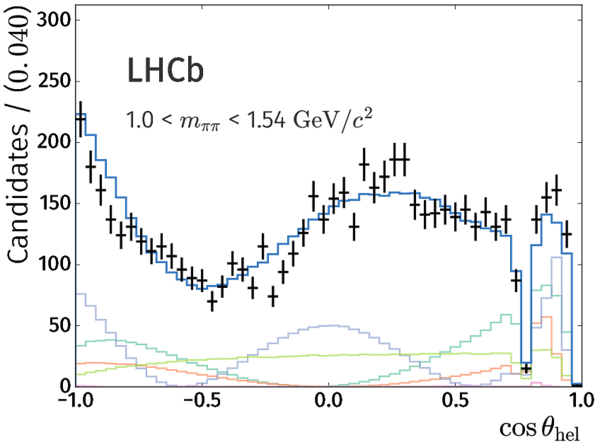
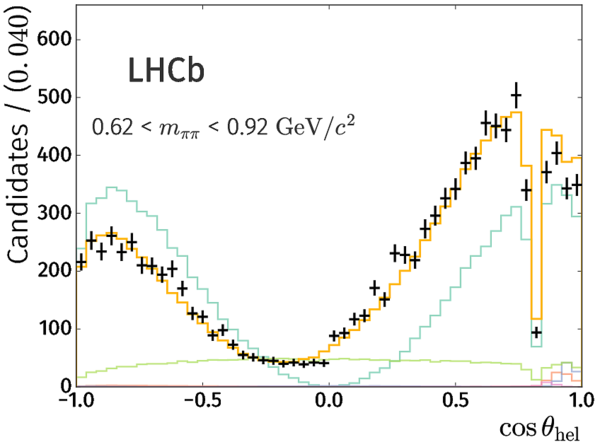
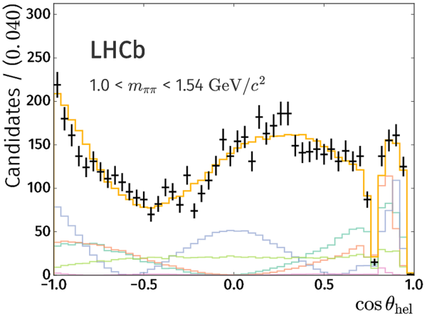
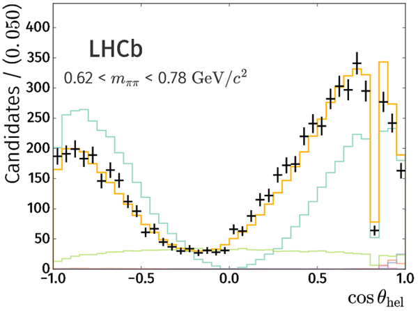
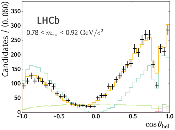
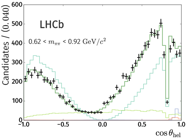
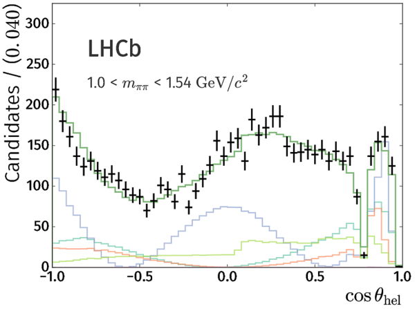
Fit projections of each model on $\cos \theta_{\rm hel}$ (a) in the region around the $\rho(770)^0$ resonance and (b) in the $f_2(1270)$ region, with the corresponding asymmetries shown beneath in (c) and (d). The pull distribution is shown below each fit projection.	Fig9.pdf [69 KiB] Thumbnail [392 KiB] *.C file
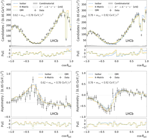
Fit projections of each model on $\cos \theta_{\rm hel}$ in the regions (a) below and (b) above the $\rho(770)^0$ resonance pole, with the corresponding asymmetries shown beneath in (c) and (d). The pull distribution is shown below each fit projection.	Fig10.pdf [63 KiB] Thumbnail [380 KiB] *.C file
Fit projections of each model (a) on $\cos \theta_{\rm hel}$ in the $\rho_3(1690)$ region, with (b) the corresponding asymmetry shown beneath. The pull distribution is shown below each fit projection.	Fig11.pdf [46 KiB] Thumbnail [392 KiB] *.C file
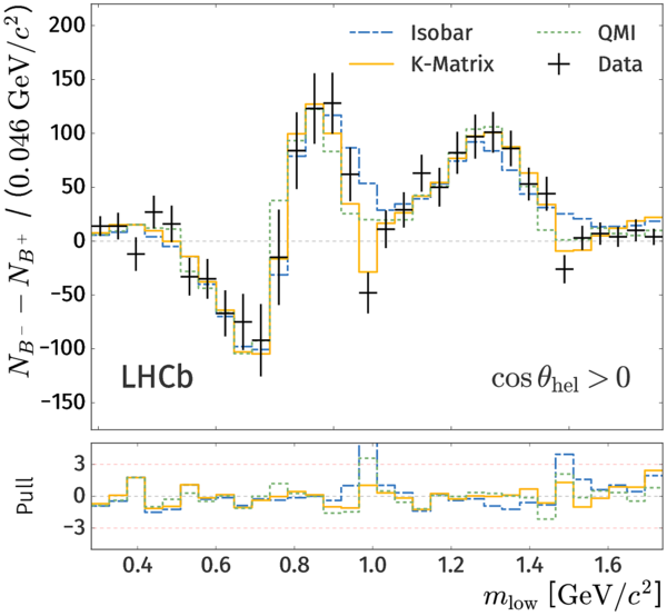
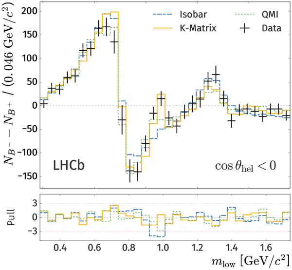
Raw difference in the number of $ B ^- $ and $ B ^+ $ candidates in the low $m_{\rm low}$ region, for (a) positive, and (b) negative cosine of the helicity angle. The pull distribution is shown below each fit projection.	Fig12a.pdf [34 KiB] Thumbnail [213 KiB] *.C file
	Fig12b.pdf [34 KiB] Thumbnail [220 KiB] *.C file
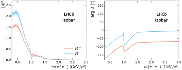
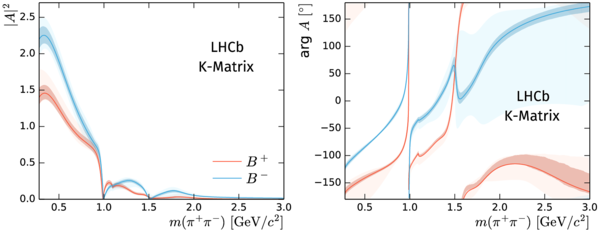
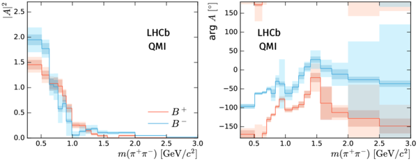
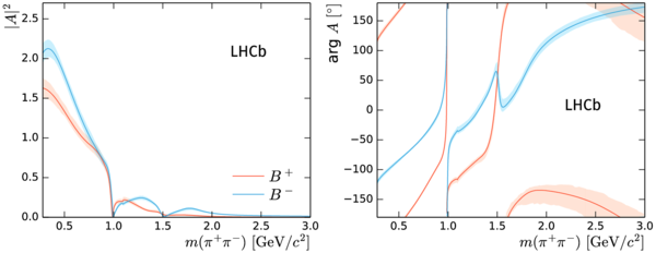
The (top) isobar, (middle) K-matrix and (bottom) QMI S-wave results where (a), (c) and (e) show the magnitude squared while (b), (d) and (f) show the phase motion. Discontinuities in the phase motion are due to presentation in the range $[-180^\circ,180^\circ]$. Red curves indicate $ B ^+ $ while blue curves represent $ B ^- $ decays, with the statistical and total uncertainties bounded by the dark and light bands, respectively (incorporating only the dominant systematic uncertainties). Note that the overall scale of the squared magnitude contains no physical meaning, but is simply a manifestation of the different scale factors and conventions adopted by each of the three amplitude analysis approaches.	Fig13a.pdf [152 KiB] HiDef png [180 KiB] Thumbnail [94 KiB] *.C file
	Fig13b.pdf [399 KiB] HiDef png [315 KiB] Thumbnail [144 KiB] *.C file
	Fig13c.pdf [30 KiB] HiDef png [132 KiB] Thumbnail [94 KiB] *.C file
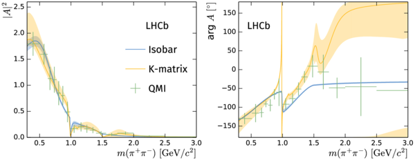
Comparison of results for the $ C P$ -averaged S-wave obtained in the three different approaches, where (a) shows the magnitude squared while (b) shows the phase motion. Discontinuities in the phase motion are due to presentation in the range $[-180^\circ,180^\circ]$. The blue curve indicates the isobar S-wave, the amber curve indicates the K-matrix S-wave, and the green points with error bars represent the QMI S-wave. The band or error bars in each case represent the total uncertainty, incorporating the dominant systematic uncertainties. As the integral of the $\|A\|^2$ plot in each approach is proportional to its respective S-wave fit fraction, the overall scale of the K-matrix and QMI plots are set relative to the isobar S-wave fit fraction in order to facilitate comparison between the three approaches.	Fig14.pdf [266 KiB] HiDef png [224 KiB] Thumbnail [115 KiB] *.C file
Data and fit model projections in the $f_2(1270)$ region with (a) freely varied $f_2(1270)$ resonance parameters, and (b) with an additional spin-$2$ component with mass and width parameters determined by the fit.	Fig15a.pdf [37 KiB] Thumbnail [225 KiB] *.C file
	Fig15b.pdf [37 KiB] Thumbnail [222 KiB] *.C file
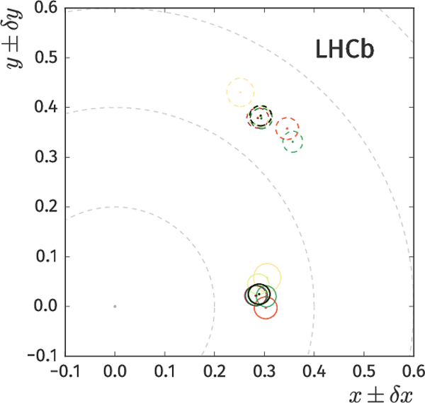
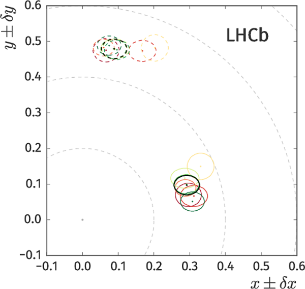
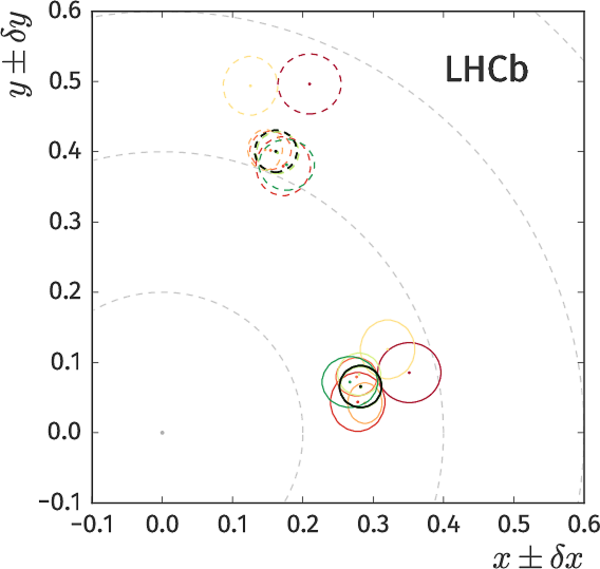
Central values (points) and statistical $68\%$ Gaussian confidence regions (ellipses) for the complex coefficients associated with the $f_2(1270)$ resonance under various systematic assumptions for the $ B ^+ $ (solid) and $ B ^- $ (dashed) decay amplitude models. The nominal result and statistical uncertainty is given in black, while the results of the dominant systematic variations to the nominal model (per Section 6) are given by the coloured ellipses, as noted in the legend, for each of the (a) isobar, (b) K-matrix and (c) QMI S-wave approaches. The model specific systematic uncertainties are discussed in Sec. 6.	Fig16a.pdf [26 KiB] HiDef png [201 KiB] Thumbnail [144 KiB] *.C file
	Fig16b.pdf [27 KiB] HiDef png [241 KiB] Thumbnail [162 KiB] *.C file
	Fig16c.pdf [26 KiB] HiDef png [250 KiB] Thumbnail [167 KiB] *.C file
	Fig16d.pdf [20 KiB] HiDef png [160 KiB] Thumbnail [128 KiB] *.C file
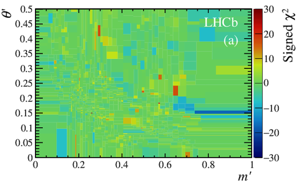
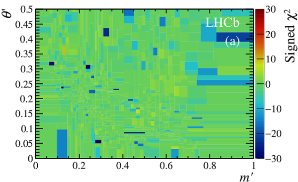
Signed $\chi^2$ distributions indicating the agreement between the isobar model fit and the data for (a) $ B ^+ $ and (b) $ B ^- $ decays.	Fig17a.pdf [49 KiB] HiDef png [482 KiB] Thumbnail [352 KiB] *.C file
	Fig17b.pdf [49 KiB] HiDef png [490 KiB] Thumbnail [352 KiB] *.C file
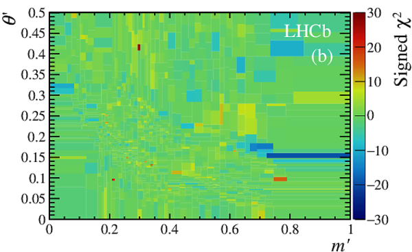
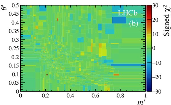
Signed $\chi^2$ distributions indicating the agreement between the K-matrix model fit and the data for (a) $ B ^+ $ and (b) $ B ^- $ decays.	Fig18a.pdf [49 KiB] HiDef png [480 KiB] Thumbnail [351 KiB] *.C file
	Fig18b.pdf [49 KiB] HiDef png [488 KiB] Thumbnail [351 KiB] *.C file
The K-matrix S-wave projections for the secondary solution, where (a) shows the magnitude-squared while (b) shows the phase motion. The red curve indicates $ B ^+ $ , while the blue curve represents $ B ^- $ decays. The light bands represent the $68\%$ confidence interval around the central values, including statistical uncertainties only.	Fig19.pdf [230 KiB] HiDef png [220 KiB] Thumbnail [109 KiB] *.C file
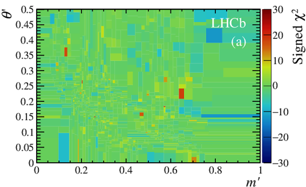
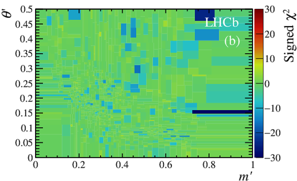
Signed $\chi^2$ distributions indicating the agreement between the QMI model fit and the data for (a) $ B ^+ $ and (b) $ B ^- $ decays.	Fig20a.pdf [49 KiB] HiDef png [482 KiB] Thumbnail [353 KiB] *.C file
	Fig20b.pdf [49 KiB] HiDef png [488 KiB] Thumbnail [352 KiB] *.C file
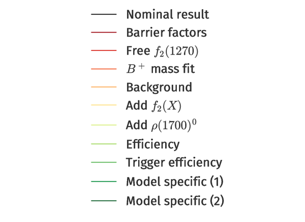
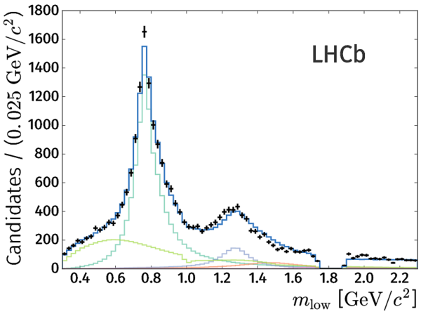
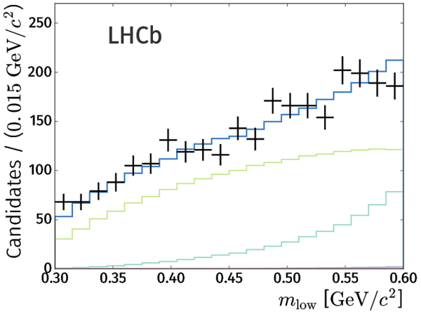
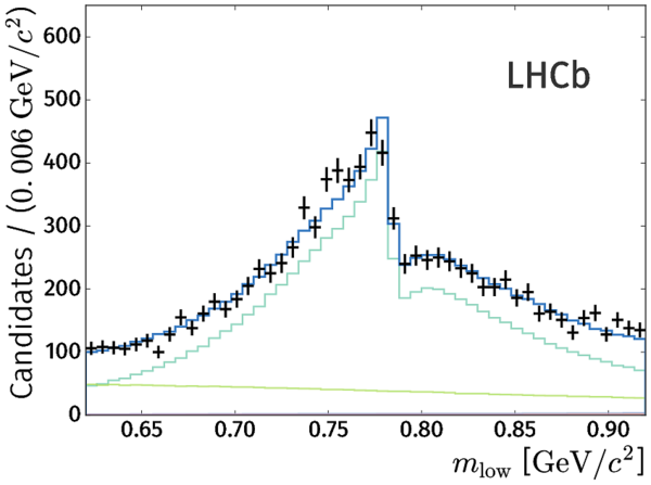
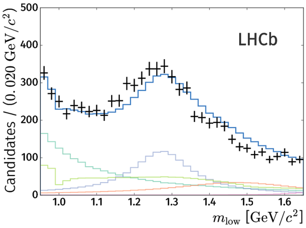
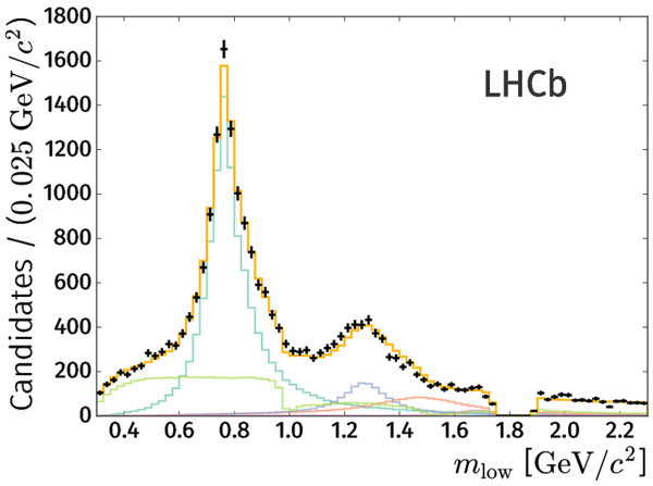
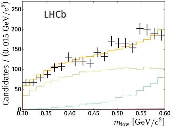
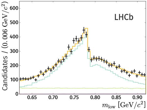
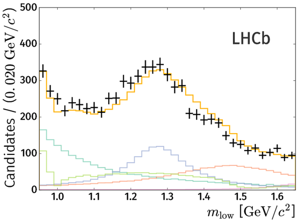
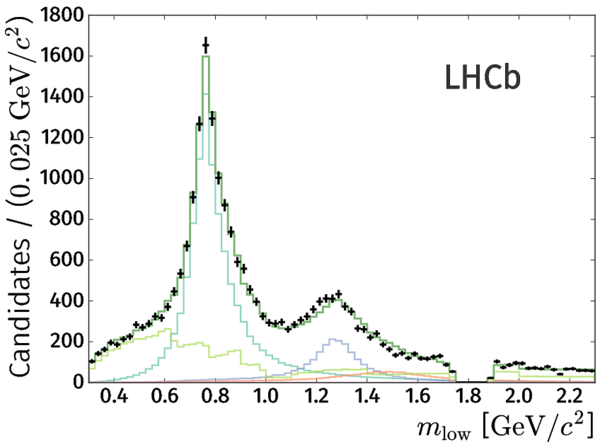
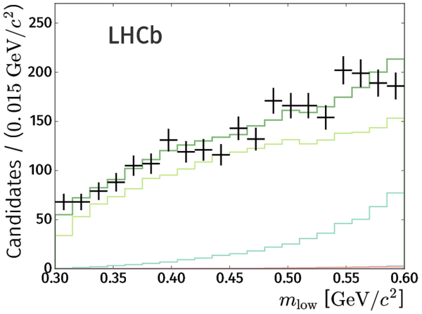
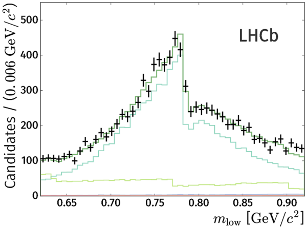
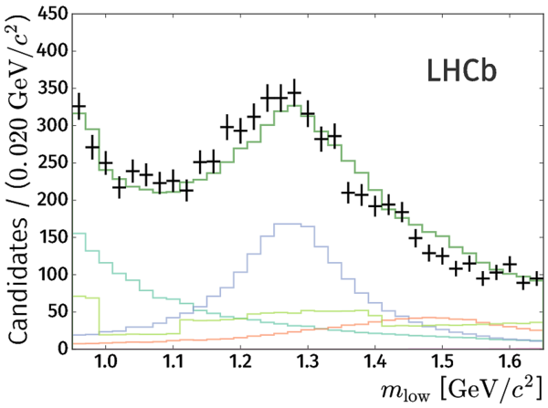
Fit projections on $m_{\rm low}$ of the result with the isobar S-wave model (a) in the low $m_{\rm low}$ region, (b) below the $\rho(770)^0$ region, (c) in the $\rho(770)^0$ region, and (d) in the $f_2(1270)$ region. The thick blue curve represents the total model, and the coloured curves represent the contributions of individual model components (not including interference effects), as per the legend in Fig. 23.	Fig21a.pdf [29 KiB] HiDef png [225 KiB] Thumbnail [170 KiB] *.C file
	Fig21b.pdf [24 KiB] HiDef png [141 KiB] Thumbnail [121 KiB] *.C file
	Fig21c.pdf [28 KiB] HiDef png [188 KiB] Thumbnail [155 KiB] *.C file
	Fig21d.pdf [25 KiB] HiDef png [164 KiB] Thumbnail [142 KiB] *.C file
Fit projections on $m_{\rm high}$ of the result with the isobar S-wave model (a) in the full $m_{\rm high}$ range, (b) in the high $m_{\rm high}$ region, and on $\cos\theta_{\rm hel}$ (c) in the $\rho(770)^0$ region and (d) in the $f_2(1270)$ region. The thick blue curve represents the total model, and the coloured curves represent the contributions of individual model components (not including interference effects), as per the legend in Fig. 23.	Fig22a.pdf [31 KiB] HiDef png [248 KiB] Thumbnail [199 KiB] *.C file
	Fig22b.pdf [26 KiB] HiDef png [183 KiB] Thumbnail [155 KiB] *.C file
	Fig22c.pdf [30 KiB] HiDef png [192 KiB] Thumbnail [152 KiB] *.C file
	Fig22d.pdf [29 KiB] HiDef png [207 KiB] Thumbnail [166 KiB] *.C file
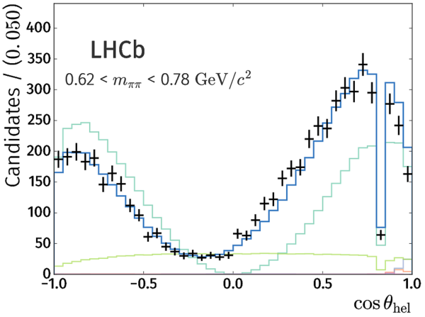
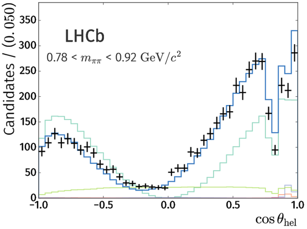
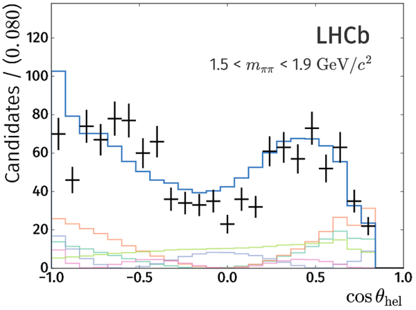
Fit projections on $\cos\theta_{\rm hel}$ of the result with the isobar S-wave model in the region (a) below and (b) above the $\rho(770)^0$ mass, and (c) in the $\rho_3(1690)^0$ region. The thick blue curve represents the total model, and the coloured curves represent the contributions of individual model components (not including interference effects), as per the legend.	Fig23a.pdf [30 KiB] HiDef png [182 KiB] Thumbnail [150 KiB] *.C file
	Fig23b.pdf [29 KiB] HiDef png [181 KiB] Thumbnail [148 KiB] *.C file
	Fig23c.pdf [28 KiB] HiDef png [156 KiB] Thumbnail [125 KiB] *.C file
	Fig23d.pdf [20 KiB] HiDef png [83 KiB] Thumbnail [67 KiB] *.C file
Fit projections on $m_{\rm low}$ of the result with the K-matrix S-wave model (a) in the low $m_{\rm low}$ region, (b) below the $\rho(770)^0$ region, (c) in the $\rho(770)^0$ region, and (d) in the $f_2(1270)$ region. The thick amber curve represents the total model, and the coloured curves represent the contributions of individual model components (not including interference effects), as per the legend in Fig. 26.	Fig24a.pdf [29 KiB] HiDef png [223 KiB] Thumbnail [168 KiB] *.C file
	Fig24b.pdf [24 KiB] HiDef png [141 KiB] Thumbnail [120 KiB] *.C file
	Fig24c.pdf [28 KiB] HiDef png [188 KiB] Thumbnail [156 KiB] *.C file
	Fig24d.pdf [25 KiB] HiDef png [164 KiB] Thumbnail [140 KiB] *.C file
Fit projections on $m_{\rm high}$ of the result with the K-matrix S-wave model (a) in the full $m_{\rm high}$ range, (b) in the high $m_{\rm high}$ region, and on $\cos\theta_{\rm hel}$ (c) in the $\rho(770)^0$ region), and (d) in the $f_2(1270)$ region. The thick amber curve represents the total model, and the coloured curves represent the contributions of individual model components (not including interference effects), as per the legend in Fig. 26.	Fig25a.pdf [31 KiB] HiDef png [253 KiB] Thumbnail [202 KiB] *.C file
	Fig25b.pdf [26 KiB] HiDef png [187 KiB] Thumbnail [158 KiB] *.C file
	Fig25c.pdf [30 KiB] HiDef png [193 KiB] Thumbnail [152 KiB] *.C file
	Fig25d.pdf [29 KiB] HiDef png [210 KiB] Thumbnail [166 KiB] *.C file
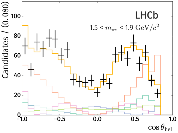
Fit projections on $\cos\theta_{\rm hel}$ of the result with the K-matrix S-wave model in the region (a) below and (b) above the $\rho(770)^0$ mass, and (c) in the $\rho_3(1690)^0$ region. The thick amber curve represents the total model, and the coloured curves represent the contributions of individual model components (not including interference effects), as per the legend.	Fig26a.pdf [30 KiB] HiDef png [182 KiB] Thumbnail [150 KiB] *.C file
	Fig26b.pdf [29 KiB] HiDef png [182 KiB] Thumbnail [148 KiB] *.C file
	Fig26c.pdf [28 KiB] HiDef png [161 KiB] Thumbnail [124 KiB] *.C file
	Fig26d.pdf [20 KiB] HiDef png [84 KiB] Thumbnail [69 KiB] *.C file
Fit projections on $m_{\rm low}$ of the result with the QMI S-wave model (a) in the low $m_{\rm low}$ region, (b) below the $\rho(770)^0$ region, (c) in the $\rho(770)^0$ region, and (d) in the $f_2(1270)$ region. The thick dark-green curve represents the total model, and the coloured curves represent the contributions of individual model components (not including interference effects), as per the legend in Fig. 29.	Fig27a.pdf [28 KiB] HiDef png [229 KiB] Thumbnail [172 KiB] *.C file
	Fig27b.pdf [24 KiB] HiDef png [144 KiB] Thumbnail [123 KiB] *.C file
	Fig27c.pdf [28 KiB] HiDef png [195 KiB] Thumbnail [160 KiB] *.C file
	Fig27d.pdf [25 KiB] HiDef png [177 KiB] Thumbnail [154 KiB] *.C file
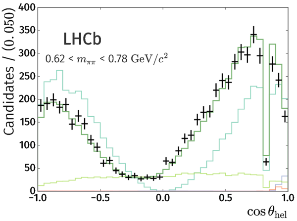
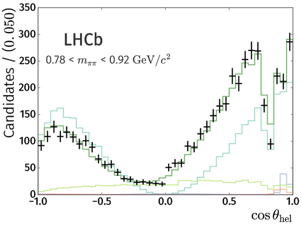
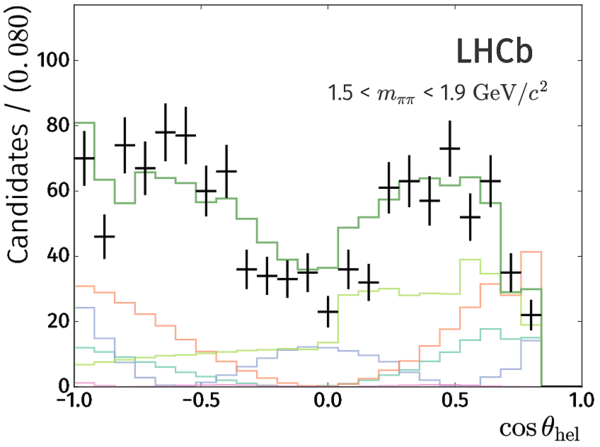
Fit projections on $m_{\rm high}$ of the result with the QMI S-wave model (a) in the full $m_{\rm high}$ range, (b) in the high $m_{\rm high}$ region, and on $\cos\theta_{\rm hel}$ in (c) the $\rho(770)^0$ region, and (d) in the $f_2(1270)$ region. The thick dark-green curve represents the total model, and the coloured curves represent the contributions of individual model components (not including interference effects), as per the legend in Fig. 29.	Fig28a.pdf [30 KiB] HiDef png [251 KiB] Thumbnail [201 KiB] *.C file
	Fig28b.pdf [26 KiB] HiDef png [186 KiB] Thumbnail [158 KiB] *.C file
	Fig28c.pdf [30 KiB] HiDef png [196 KiB] Thumbnail [155 KiB] *.C file
	Fig28d.pdf [29 KiB] HiDef png [205 KiB] Thumbnail [163 KiB] *.C file
Fit projections on $\cos\theta_{\rm hel}$ of the result with the QMI S-wave model in the region (a) below and (b) above the $\rho(770)^0$ mass, and (c) in the $\rho_3(1690)^0$ region. The thick dark-green curve represents the total model, and the coloured curves represent the contributions of individual model components (not including interference effects), as per the legend.	Fig29a.pdf [30 KiB] HiDef png [184 KiB] Thumbnail [150 KiB] *.C file
	Fig29b.pdf [29 KiB] HiDef png [185 KiB] Thumbnail [150 KiB] *.C file
	Fig29c.pdf [28 KiB] HiDef png [156 KiB] Thumbnail [122 KiB] *.C file
	Fig29d.pdf [20 KiB] HiDef png [82 KiB] Thumbnail [65 KiB] *.C file
Animated gif made out of all figures.	PAPER-2019-017.gif Thumbnail

Tables and captions

Component yields and phase-space-integrated raw detection asymmetries in the $ B ^+ $ signal region, calculated from the results of the invariant-mass fit. The uncertainties include both statistical and systematic effects.	Table_1.pdf [59 KiB] HiDef png [60 KiB] Thumbnail [29 KiB] tex code
K-matrix parameters quoted in Ref. [77], which are obtained from a global analysis of $\pi\pi$ scattering data [74]. Only $f_{1v}$ parameters are listed here, since only the dipion final state is relevant to the analysis. Masses $m_\alpha$ and couplings $g_u^{\alpha}$ are given in $ \text{ Ge V} $, while units of $ \text{ Ge V} ^2$ for $s$-related quantities are implied; $s^{\rm{prod}}_0$ is taken from Ref. [76].	Table_2.pdf [65 KiB] HiDef png [96 KiB] Thumbnail [41 KiB] tex code
Non-S-wave resonances and their default lineshapes as identified by the model selection procedure. These are common to all S-wave approaches.	Table_3.pdf [47 KiB] HiDef png [64 KiB] Thumbnail [29 KiB] tex code
Systematic uncertainties on the $ C P$ -averaged fit fractions, given in units of $10^{-2}$, for the isobar method. Uncertainties are given both for the total S-wave, and for the individual components due to the $\sigma$ pole and the rescattering amplitude. For comparison, the statistical uncertainties are also listed at the bottom.	Table_4.pdf [66 KiB] HiDef png [125 KiB] Thumbnail [53 KiB] tex code
Systematic uncertainties on ${\cal A}_{ C P }$ values, given in units of $10^{-2}$, for the isobar method. Uncertainties are given both for the total S-wave, and for the individual components due to the $\sigma$ pole and the rescattering amplitude. For comparison, the statistical uncertainties are also listed at the bottom.	Table_5.pdf [66 KiB] HiDef png [128 KiB] Thumbnail [53 KiB] tex code
Systematic uncertainties on the $ C P$ -averaged fit fractions, given in units of $10^{-2}$, for the K-matrix method. For comparison, the statistical uncertainties are also listed at the bottom.	Table_6.pdf [66 KiB] HiDef png [140 KiB] Thumbnail [63 KiB] tex code
Systematic uncertainties on ${\cal A}_{ C P }$ values, given in units of $10^{-2}$, for the K-matrix method. For comparison, the statistical uncertainties are also listed at the bottom.	Table_7.pdf [66 KiB] HiDef png [139 KiB] Thumbnail [62 KiB] tex code
Systematic uncertainties on the $ C P$ -averaged fit fractions, given in units of $10^{-2}$, for the QMI method. For comparison, the statistical uncertainties are also listed at the bottom.	Table_8.pdf [66 KiB] HiDef png [133 KiB] Thumbnail [59 KiB] tex code
Systematic uncertainties on ${\cal A}_{ C P }$ values, given in units of $10^{-2}$, for the QMI method. For comparison, the statistical uncertainties are also listed at the bottom.	Table_9.pdf [66 KiB] HiDef png [133 KiB] Thumbnail [60 KiB] tex code
The $ C P$ -separated sum of fit fractions in units of $10^{-2}$, for each approach, where the first uncertainty is statistical, the second the experimental systematic and the third is the model systematic.	Table_10.pdf [58 KiB] HiDef png [36 KiB] Thumbnail [18 KiB] tex code
The $ C P$ -averaged fit fractions in units of $10^{-2}$, for each approach, where the first uncertainty is statistical, the second the experimental systematic and the third is the model systematic.	Table_11.pdf [53 KiB] HiDef png [55 KiB] Thumbnail [27 KiB] tex code
Fit (diagonal) and interference (off-diagonal) fractions for $ B ^+ $ decay in units of $10^{-2}$, between amplitude components in the isobar approach. The first uncertainty is statistical and the second the quadratic sum of systematic and model sources.	Table_12.pdf [51 KiB] HiDef png [40 KiB] Thumbnail [17 KiB] tex code
Fit (diagonal) and interference (off-diagonal) fractions for $ B ^- $ decay in units of $10^{-2}$, between amplitude components in the isobar approach. The first uncertainty is statistical and the second the quadratic sum of systematic and model sources.	Table_13.pdf [51 KiB] HiDef png [40 KiB] Thumbnail [17 KiB] tex code
Fit (diagonal) and interference (off-diagonal) fractions for $ B ^+ $ decay in units of $10^{-2}$, between amplitude components in the K-matrix approach. The first uncertainty is statistical and the second the quadratic sum of systematic and model sources.	Table_14.pdf [50 KiB] HiDef png [37 KiB] Thumbnail [17 KiB] tex code
Fit (diagonal) and interference (off-diagonal) fractions for $ B ^- $ decay in units of $10^{-2}$, between amplitude components in the K-matrix approach. The first uncertainty is statistical and the second the quadratic sum of systematic and model sources.	Table_15.pdf [50 KiB] HiDef png [36 KiB] Thumbnail [17 KiB] tex code
Fit (diagonal) and interference (off-diagonal) fractions for $ B ^+ $ decay in units of $10^{-2}$, between amplitude components in the QMI approach. The first uncertainty is statistical and the second the quadratic sum of systematic and model sources.	Table_16.pdf [50 KiB] HiDef png [37 KiB] Thumbnail [17 KiB] tex code
Fit (diagonal) and interference (off-diagonal) fractions for $ B ^- $ decay in units of $10^{-2}$, between amplitude components in the QMI approach. The first uncertainty is statistical and the second the quadratic sum of systematic and model sources.	Table_17.pdf [50 KiB] HiDef png [37 KiB] Thumbnail [17 KiB] tex code
Quasi-two-body $ C P$ asymmetries in units of $10^{-2}$, for each approach. The first uncertainty is statistical, the second the experimental systematic and the third is the model systematic.	Table_18.pdf [54 KiB] HiDef png [56 KiB] Thumbnail [27 KiB] tex code
QMI S-wave fit results where the first uncertainty is statistical and the second the quadratic sum of systematic and model sources.	Table_19.pdf [67 KiB] HiDef png [160 KiB] Thumbnail [77 KiB] tex code
The obtained $\rho(770)^0$ mass and width parameters, for each approach, where the uncertainty is statistical.	Table_20.pdf [52 KiB] HiDef png [40 KiB] Thumbnail [19 KiB] tex code
Cartesian coefficients, $c_j$, for the components of the isobar model fit.	Table_21.pdf [54 KiB] HiDef png [71 KiB] Thumbnail [30 KiB] tex code
Fitted values of the pole parameters in the isobar model fit.	Table_22.pdf [48 KiB] HiDef png [54 KiB] Thumbnail [23 KiB] tex code
Statistical correlation matrix for the isobar model $ C P$ -averaged fit fractions.	Table_23.pdf [51 KiB] HiDef png [40 KiB] Thumbnail [19 KiB] tex code
Systematic correlation matrix for the isobar model $ C P$ -averaged fit fractions.	Table_24.pdf [51 KiB] HiDef png [42 KiB] Thumbnail [19 KiB] tex code
Statistical correlation matrix for the isobar model quasi-two-body decay $ C P$ asymmetries.	Table_25.pdf [51 KiB] HiDef png [42 KiB] Thumbnail [19 KiB] tex code
Systematic correlation matrix for the isobar model quasi-two-body decay $ C P$ asymmetries.	Table_26.pdf [51 KiB] HiDef png [43 KiB] Thumbnail [19 KiB] tex code
Cartesian coefficients, $c_j$, for the components of the K-matrix model fit. For the K-matrix model, the $\beta_{\alpha}$ and $f^{\rm prod}_{v}$ parameters describe the relative contributions of the production pole $\alpha$ and production slowly varying part corresponding to channel $v$, respectively. In the absence of $ C P$ violation, $\delta x = \delta y = 0$.	Table_27.pdf [54 KiB] HiDef png [149 KiB] Thumbnail [60 KiB] tex code
Statistical correlation matrix for the K-matrix $ C P$ -averaged fit fractions.	Table_28.pdf [50 KiB] HiDef png [45 KiB] Thumbnail [21 KiB] tex code
Systematic correlation matrix for the K-matrix $ C P$ -averaged fit fractions.	Table_29.pdf [50 KiB] HiDef png [46 KiB] Thumbnail [21 KiB] tex code
Statistical correlation matrix for the K-matrix quasi-two-body decay $ C P$ asymmetries.	Table_30.pdf [50 KiB] HiDef png [44 KiB] Thumbnail [20 KiB] tex code
Systematic correlation matrix for the K-matrix quasi-two-body decay $ C P$ asymmetries.	Table_31.pdf [43 KiB] HiDef png [45 KiB] Thumbnail [21 KiB] tex code
Isobar coefficients, $c_j$, for the components of the second solution of the K-matrix model fit, where uncertainties are statistical only. For the K-matrix model, the $\beta_{\alpha}$ and $f^{\rm prod}_{v}$ parameters describe the relative contributions of the production pole $\alpha$ and production slowly varying part corresponding to channel $v$, respectively. In the absence of $ C P$ violation, $\delta x = \delta y = 0$.	Table_32.pdf [54 KiB] HiDef png [149 KiB] Thumbnail [65 KiB] tex code
Cartesian coefficients obtained with the QMI model. Only the statistical uncertainties are shown as some systematic variations change the overall scale of various lineshapes at this level.	Table_33.pdf [52 KiB] HiDef png [58 KiB] Thumbnail [26 KiB] tex code
Statistical correlation matrix for the QMI $ C P$ -averaged fit fractions.	Table_34.pdf [50 KiB] HiDef png [44 KiB] Thumbnail [20 KiB] tex code
Correlation matrix corresponding to the quadratic sum of systematic and model uncertainties for the QMI fit $ C P$ -averaged fractions.	Table_35.pdf [50 KiB] HiDef png [44 KiB] Thumbnail [21 KiB] tex code
Statistical correlation matrix for the QMI quasi-two-body decay $ C P$ asymmetries.	Table_36.pdf [50 KiB] HiDef png [45 KiB] Thumbnail [21 KiB] tex code
Correlation matrix corresponding to the quadratic sum of systematic and model uncertainties for the QMI quasi-two-body decay $ C P$ asymmetries.	Table_37.pdf [50 KiB] HiDef png [44 KiB] Thumbnail [21 KiB] tex code
Results with S-wave model variation included as a source of systematic uncertainty. The first uncertainty is statistical, the second is experimental systematic and the third is the adjusted model systematic uncertainty.	Table_38.pdf [61 KiB] HiDef png [55 KiB] Thumbnail [27 KiB] tex code
Phase comparison in degrees for (top) $ B ^+ $ and (bottom) $ B ^- $ between the three S-wave approaches where the first uncertainty is statistical, the second systematic and the third from the model. Note that the phase of the $\rho(770)^0$ component of the $\rho$--$\omega$ lineshape is fixed to zero as it is selected to be the reference contribution.	Table_39.pdf [53 KiB] HiDef png [83 KiB] Thumbnail [45 KiB] tex code