Measurement of CP violation in the $B_s^0\rightarrow\phi\phi$ decay and search for the $B^0\rightarrow\phi\phi$ decay

Information

LHCb-PAPER-2019-019
CERN-EP-2019-121
arXiv:1907.10003 [PDF]

(Submitted on 23 Jul 2019)
JHEP 12 (2019) 155
Inspire 1745979

Tools

Abstract

A measurement of the time-dependent CP-violating asymmetry in $B_s^0\rightarrow\phi\phi$ decays is presented. Using a sample of proton-proton collision data corresponding to an integrated luminosity of $5.0$fb$^{-1}$ collected by the $ LHCb$ experiment at centre-of-mass energies $\sqrt{s} = 7$ TeV in 2011, 8 TeV in 2012 and 13 TeV in 2015 and 2016, a signal yield of around 9000 $B_s^0\rightarrow\phi\phi$ decays is obtained. The CP-violating phase $\phi_s^{s\bar{s}s}$ is measured to be $-0.073 \pm 0.115$(stat)$\pm 0.027$(syst) rad, under the assumption it is independent on the helicity of the $\phi\phi$ decay. In addition, the CP-violating phases of the transverse polarisations under the assumption of CP conservation of the longitudinal phase are measured. The helicity-independent direct CP-violation parameter is also measured, and is found to be $|\lambda|=0.99 \pm 0.05 $(stat)$ \pm 0.01 $(syst). In addition, $T$-odd triple-product asymmetries are measured. The results obtained are consistent with the hypothesis of CP conservation in $b\rightarrow\bar{s}s\bar{s}$ transitions. Finally, a limit on the branching fraction of the $B^0\rightarrow \phi\phi$ decay is determined to be $\mathcal{B}(B^0\rightarrow \phi\phi)<2.7\times 10^{-8}$ at 90 confidence level.

Figures and captions

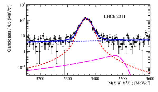
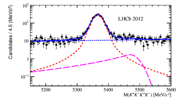
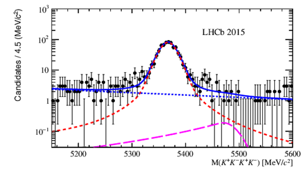
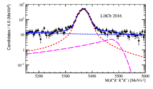
A fit to the four-kaon mass for the (top left) 2011, (top right) 2012, (bottom left) 2015 and (bottom right) 2016 data sets, which are represented by the black points. Also shown are the results of the total fit (blue solid line), with the $ B ^0_ s \rightarrow \phi\phi$ (red dashed), the $\Lambda ^0_ b \rightarrow \phi p K ^- $ (magenta long dashed), and the combinatorial (blue short dashed) fit components.	Fig1a.pdf [26 KiB] HiDef png [207 KiB] Thumbnail [179 KiB] *.C file
	Fig1b.pdf [26 KiB] HiDef png [197 KiB] Thumbnail [168 KiB] *.C file
	Fig1c.pdf [25 KiB] HiDef png [218 KiB] Thumbnail [186 KiB] *.C file
	Fig1d.pdf [26 KiB] HiDef png [199 KiB] Thumbnail [168 KiB] *.C file
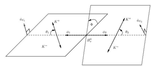
Decay angles for the $ B ^0_ s \rightarrow \phi \phi$ decay, where $\theta_{1,2}$ is the angle between the $K^+$ momentum in the $\phi_{1,2}$ meson rest frame and the $\phi_{1,2}$ momentum in the $ B ^0_ s $ rest frame, $\Phi$ is the angle between the two $\phi$ meson decay planes and $\hat{n}_{V_{1,2}}$ is the unit vector normal to the decay plane of the $\phi_{1,2}$ meson.	Fig_2.pdf [72 KiB] HiDef png [58 KiB] Thumbnail [35 KiB] *.C file tex code
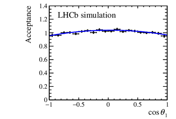
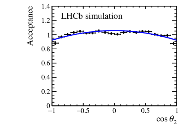
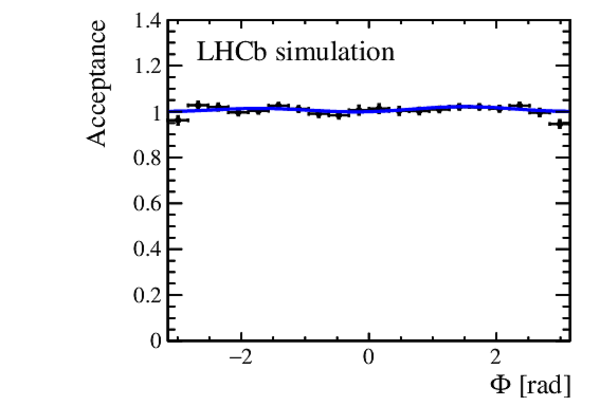
Angular acceptance normalised to the average obtained using simulated $ B ^0_ s \rightarrow \phi\phi$ decays (top-left) integrated over $\cos\theta_2$ and $\Phi$ as a function of $\cos\theta_1$, (top-right) integrated over $\cos\theta_1$ and $\Phi$ as a function of $\cos\theta_2$, and (bottom) integrated over $\cos\theta_1$ and $\cos\theta_2$ as a function of $\Phi$. Each figure includes the resulting fit curve.	Fig3a.pdf [15 KiB] HiDef png [103 KiB] Thumbnail [96 KiB] *.C file
	Fig3b.pdf [15 KiB] HiDef png [107 KiB] Thumbnail [100 KiB] *.C file
	Fig3c.pdf [15 KiB] HiDef png [97 KiB] Thumbnail [90 KiB] *.C file
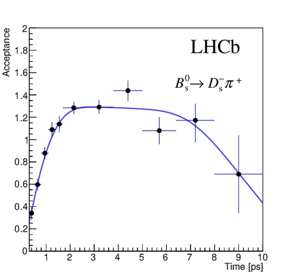
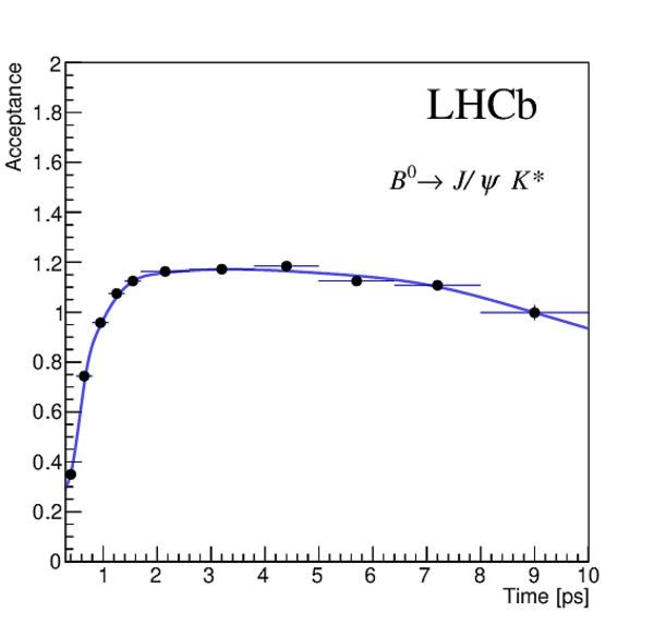
Decay-time acceptances calculated from (left) $ B ^0_ s \rightarrow D ^-_ s \pi ^+ $ decays to match Run 1 data and (right) $ B ^0 \rightarrow { J \mskip -3mu/\mskip -2mu\psi \mskip 2mu} K ^{*0} $ decays to match Run 2 data. Superimposed is a parameterisation using cubic splines..	Fig4a.pdf [15 KiB] HiDef png [165 KiB] Thumbnail [121 KiB] *.C file
	Fig4b.pdf [15 KiB] HiDef png [147 KiB] Thumbnail [110 KiB] *.C file
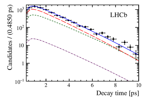
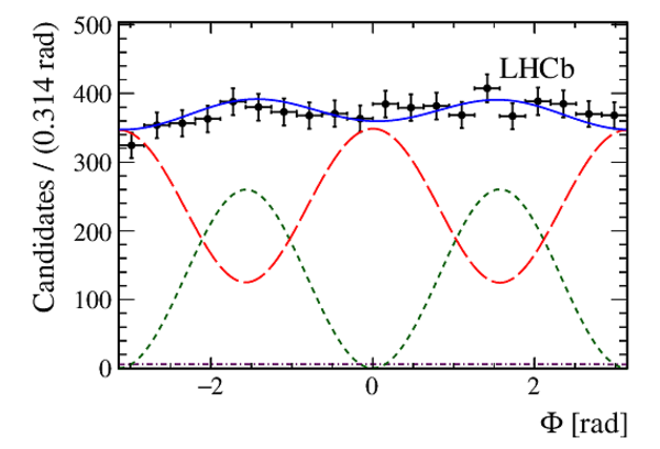
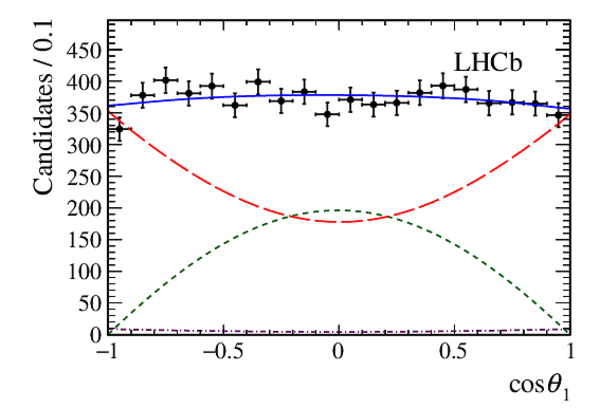
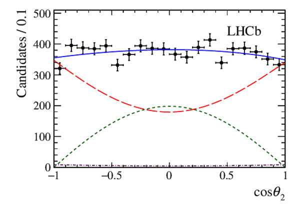
One-dimensional projections of the $ B ^0_ s \rightarrow \phi\phi$ fit for (top-left) decay time with binned acceptance, (top-right) helicity angle $\Phi$ and (bottom-left and bottom-right) cosine of the helicity angles $\theta_1$ and $\theta_2$. The background-subtracted data are marked as black points, while the blue solid lines represent the projections of the fit. The $ C P$ -even $P$-wave, the $ C P$ -odd $P$-wave and the combined $S$-wave and double $S$-wave components are shown by the red long dashed, green short dashed and purple dot-dashed lines, respectively. Fitted components are plotted taking into account efficiencies in the time and angular observables.	Fig5a.pdf [16 KiB] HiDef png [191 KiB] Thumbnail [153 KiB] *.C file
	Fig5b.pdf [18 KiB] HiDef png [202 KiB] Thumbnail [162 KiB] *.C file
	Fig5c.pdf [17 KiB] HiDef png [193 KiB] Thumbnail [169 KiB] *.C file
	Fig5d.pdf [16 KiB] HiDef png [179 KiB] Thumbnail [150 KiB] *.C file
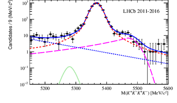
Fit to the four-kaon invariant mass. The total PDF as described in the text is shown as a blue solid line, $ B ^0_ s \rightarrow \phi\phi$ as a red dashed line, $ B ^0 \rightarrow \phi \phi$ as a green dotted line, the $\Lambda ^0_ b \rightarrow \phi p K$ contribution as a magenta long-dashed line and the combinatorial background as a blue short-dashed line.	Fig6.pdf [22 KiB] HiDef png [218 KiB] Thumbnail [173 KiB] *.C file
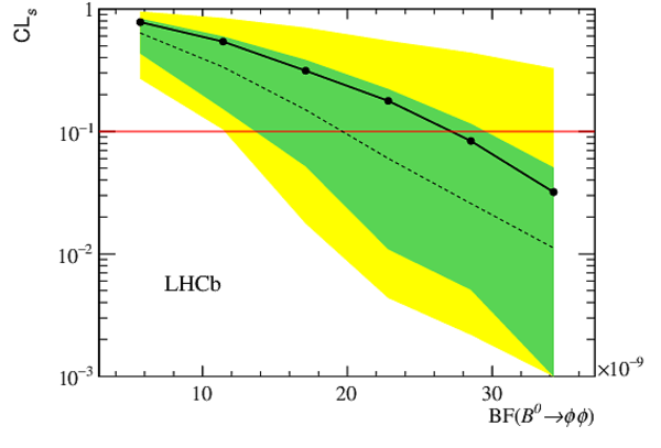
Results of the ${\rm CL}_s$ scan as a function of the $ B ^0 \rightarrow\phi\phi$ yield. The solid black line shows the observed ${\rm CL}_s$ distribution, while the dotted black line indicates the expected distribution. The green (yellow) band marks the $1\sigma$ ($2\sigma$) confidence region on the expected ${\rm CL}_s$. The $90 \%$ CL limit is shown as a red line.	Fig7.pdf [13 KiB] HiDef png [182 KiB] Thumbnail [130 KiB] *.C file
Animated gif made out of all figures.	PAPER-2019-019.gif Thumbnail

Tables and captions

Angular coefficients, written in the same basis as the efficiency parameterisation.	Table_1.pdf [76 KiB] HiDef png [114 KiB] Thumbnail [52 KiB] tex code
Tagging performance of the opposite-side (OS) and same-side kaon (SSK) flavour taggers for the $ B ^0_ s \rightarrow \phi\phi$ decay.	Table_2.pdf [53 KiB] HiDef png [86 KiB] Thumbnail [40 KiB] tex code
Results of the decay-time-dependent, polarisation-independent fit for the $ C P$ -violation fit. Uncertainties shown do not include systematic contributions.	Table_3.pdf [67 KiB] HiDef png [122 KiB] Thumbnail [52 KiB] tex code
Results of the polarisation-dependent fit for the $ C P$ violation fit. Uncertainties shown do not include systematic contributions.	Table_4.pdf [58 KiB] HiDef png [70 KiB] Thumbnail [28 KiB] tex code
Summary of systematic uncertainties (in units of $10^{-2}$) for parameters of interest in the decay-time-dependent measurement.	Table_5.pdf [70 KiB] HiDef png [63 KiB] Thumbnail [30 KiB] tex code
Summary of systematic uncertainties on $A_U$ and $A_V$.	Table_6.pdf [32 KiB] HiDef png [86 KiB] Thumbnail [37 KiB] tex code
Coefficients of the time-dependent terms and angular functions used in Eq. ???. Amplitudes are defined at $t=0$.	Table_7.pdf [96 KiB] HiDef png [166 KiB] Thumbnail [73 KiB] tex code
Statistical correlation matrix of the time-dependent fit.	Table_8.pdf [64 KiB] HiDef png [48 KiB] Thumbnail [26 KiB] tex code
Statistical correlation matrix of the time-dependent fit in which $ C P$ violation is polarisation dependent.	Table_9.pdf [64 KiB] HiDef png [47 KiB] Thumbnail [26 KiB] tex code