Amplitude analysis of the $B^+ \to D^+ D^- K^+$ decay

Information

LHCb-PAPER-2020-025
CERN-EP-2020-159
arXiv:2009.00026 [PDF]

(Submitted on 31 Aug 2020)
Phys. Rev. D102 (2020) 112003
Inspire 1814324

Tools

Abstract

Results are reported from an amplitude analysis of the $B^+\to D^+D^-K^+$ decay. The analysis is carried out using LHCb proton-proton collision data taken at $\sqrt{s}=7,8,$ and $13$ TeV, corresponding to a total integrated luminosity of 9 fb$^{-1}$. In order to obtain a good description of the data, it is found to be necessary to include new spin-0 and spin-1 resonances in the $D^-K^+$ channel with masses around 2.9 GeV$/c^2$, and a new spin-0 charmonium resonance in proximity to the spin-2 $\chi_{c2}(3930)$ state. The masses and widths of these resonances are determined, as are the relative contributions of all components in the amplitude model, which additionally include the vector charmonia $\psi(3770)$, $\psi(4040)$, $\psi(4160)$ and $\psi(4415)$ states and a nonresonant component.

Figures and captions

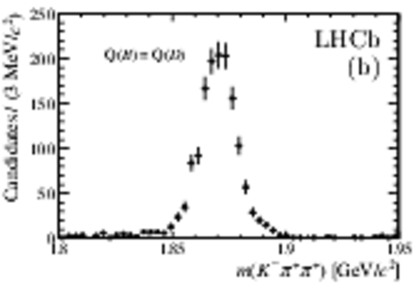
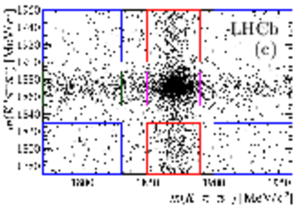
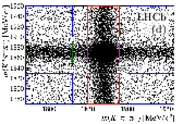
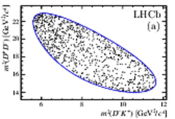
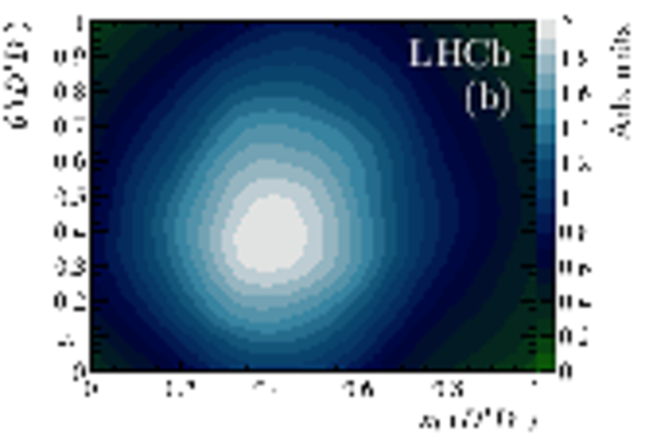
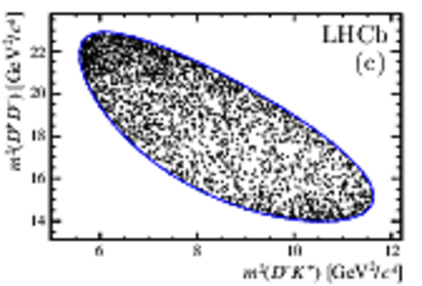
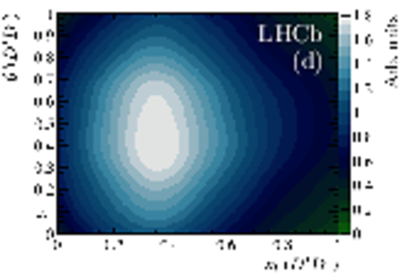
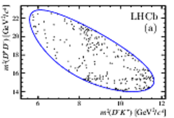
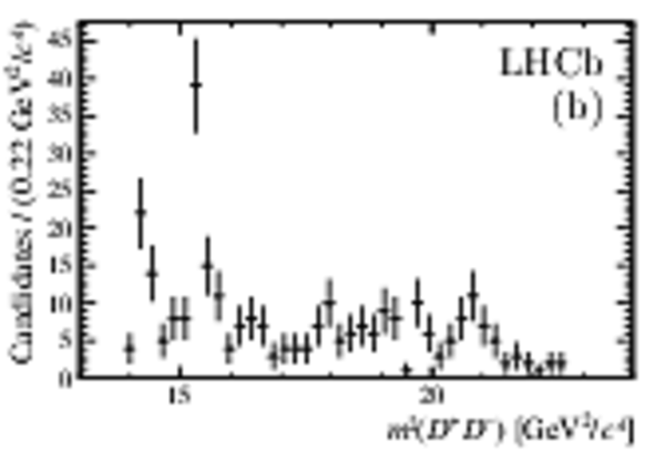
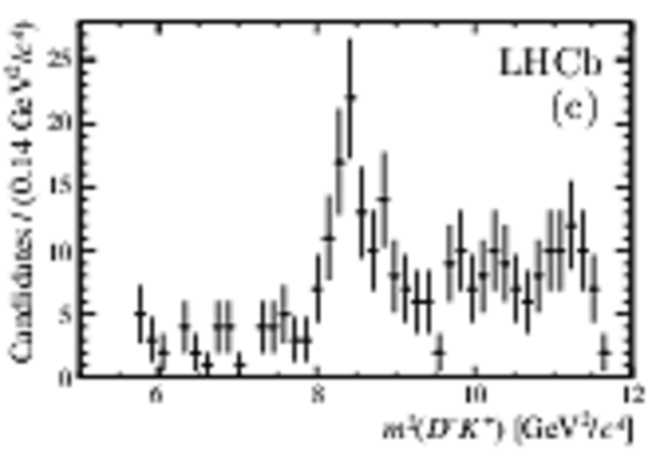
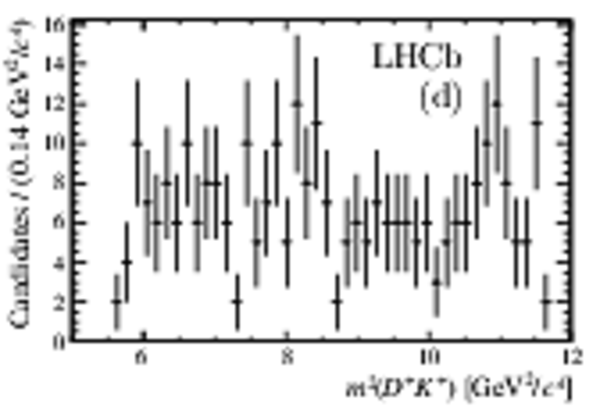
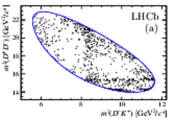
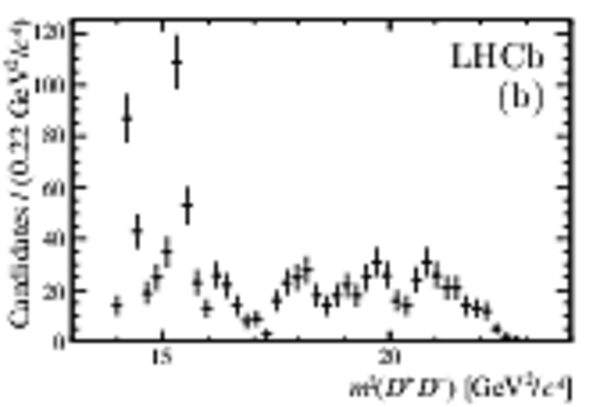
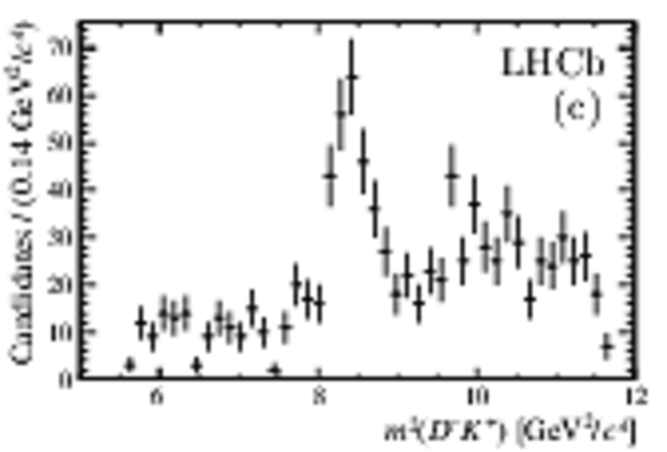
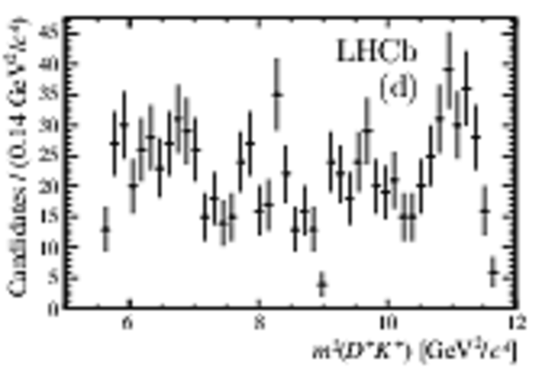
Invariant-mass distributions for the selected candidates for the $D$ meson having (a) the opposite and (b) the same charge, $Q$, as the $B$ meson, and in the two-dimensional plane showing the two invariant masses in (c) Run 1 and (d) Run 2 data. In (c) and (d) the blue rectangles correspond to regions of charmless background and the green and red where both single-charm and charmless processes contribute. The magenta rectangle indicates the signal region.	fig1a.pdf [24 KiB] HiDef png [170 KiB] Thumbnail [115 KiB] *.C file
	fig1b.pdf [23 KiB] HiDef png [171 KiB] Thumbnail [114 KiB] *.C file
	fig1c.pdf [47 KiB] HiDef png [739 KiB] Thumbnail [565 KiB] *.C file
	fig1d.pdf [77 KiB] HiDef png [1 MiB] Thumbnail [847 KiB] *.C file
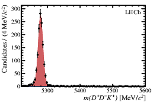
Invariant-mass distribution for $ B $ candidates with the results of the fit superimposed, where the signal component is indicated in red and background (barely visible) in blue.	fig2.pdf [39 KiB] HiDef png [183 KiB] Thumbnail [226 KiB] *.C file
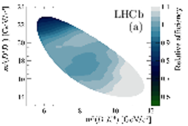
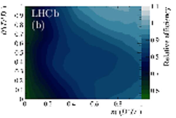
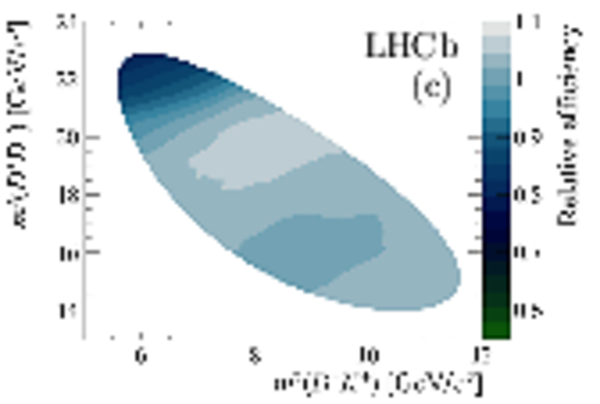
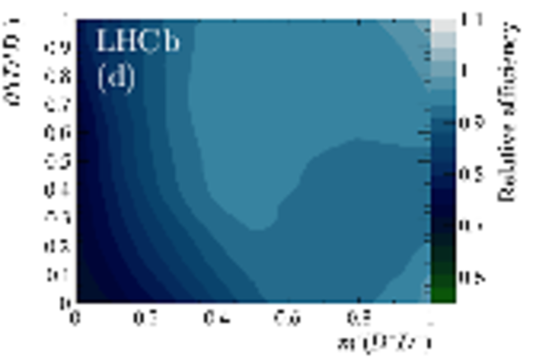
Efficiency maps for (upper) Run 1 and (lower) Run 2, where the variation as a function of position in the (left) standard Dalitz plot and (right) SDP are shown. The $z$-axis scale is arbitrary as the absolute efficiency does not affect the analysis.	fig3a.pdf [89 KiB] HiDef png [484 KiB] Thumbnail [337 KiB] *.C file
	fig3b.pdf [94 KiB] HiDef png [740 KiB] Thumbnail [449 KiB] *.C file
	fig3c.pdf [87 KiB] HiDef png [441 KiB] Thumbnail [321 KiB] *.C file
	fig3d.pdf [89 KiB] HiDef png [594 KiB] Thumbnail [376 KiB] *.C file
Visualisation of the sideband candidates in the (a,c) standard Dalitz plot and (b,d) derived background models in the SDP for (a,b) Run 1 and (c,d) Run 2 data.	fig4a.pdf [111 KiB] HiDef png [445 KiB] Thumbnail [488 KiB] *.C file
	fig4b.pdf [26 KiB] HiDef png [884 KiB] Thumbnail [606 KiB] *.C file
	fig4c.pdf [173 KiB] HiDef png [655 KiB] Thumbnail [553 KiB] *.C file
	fig4d.pdf [26 KiB] HiDef png [871 KiB] Thumbnail [608 KiB] *.C file
Run 1 data entering the amplitude fit, shown in the Dalitz plot and its projection onto the invariant-mass squared for each of the three pairs of the final-state particles.	fig5a.pdf [90 KiB] HiDef png [306 KiB] Thumbnail [361 KiB] *.C file
	fig5b.pdf [24 KiB] HiDef png [176 KiB] Thumbnail [132 KiB] *.C file
	fig5c.pdf [24 KiB] HiDef png [162 KiB] Thumbnail [139 KiB] *.C file
	fig5d.pdf [24 KiB] HiDef png [174 KiB] Thumbnail [152 KiB] *.C file
Run 2 data entering the amplitude fit, shown in the Dalitz plot and its projection onto the invariant-mass squared for each of the three pairs of the final-state particles.	fig6a.pdf [113 KiB] HiDef png [413 KiB] Thumbnail [443 KiB] *.C file
	fig6b.pdf [24 KiB] HiDef png [158 KiB] Thumbnail [121 KiB] *.C file
	fig6c.pdf [25 KiB] HiDef png [178 KiB] Thumbnail [143 KiB] *.C file
	fig6d.pdf [25 KiB] HiDef png [187 KiB] Thumbnail [155 KiB] *.C file
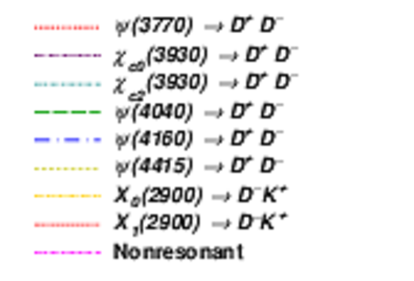
Comparisons of the invariant-mass distributions of $ B ^+ \rightarrow D ^+ D ^- K ^+ $ candidates to the fit projections without any resonant component in the $ D ^- K ^+ $ channel. The total fit function (solid black line) and contributions from individual components (non-solid coloured lines) are shown as detailed in the legend.	fig7a.pdf [117 KiB] HiDef png [420 KiB] Thumbnail [362 KiB] *.C file
	fig7b.pdf [121 KiB] HiDef png [423 KiB] Thumbnail [410 KiB] *.C file
	fig7c.pdf [127 KiB] HiDef png [453 KiB] Thumbnail [445 KiB] *.C file
	fig7d.pdf [11 KiB] HiDef png [287 KiB] Thumbnail [353 KiB] *.C file
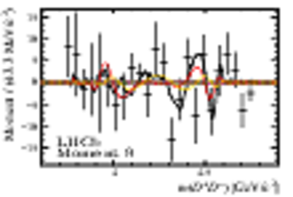
Normalised residual between the data and the model excluding any $ D ^- K ^+ $ components, shown across the Dalitz plot with a minimum of 20 data entries in each bin.	fig8.pdf [105 KiB] HiDef png [559 KiB] Thumbnail [453 KiB] *.C file
Comparison of the $m( D ^- K ^+ )$ distribution and the fit projection for a model excluding any $ D ^- K ^+ $ resonance, after requiring $m( D ^+ D ^- )>4\text{ Ge V /}c^2 $ to suppress reflections from charmonium resonances. The different components are shown as indicated in the legend of Fig. ???.	fig9.pdf [127 KiB] HiDef png [247 KiB] Thumbnail [277 KiB] *.C file
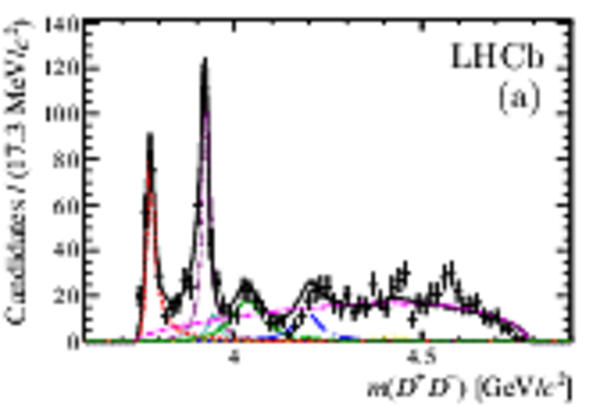
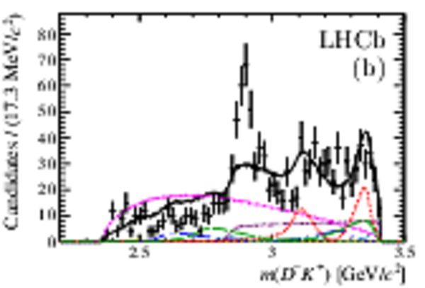
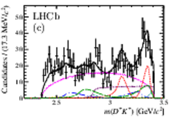
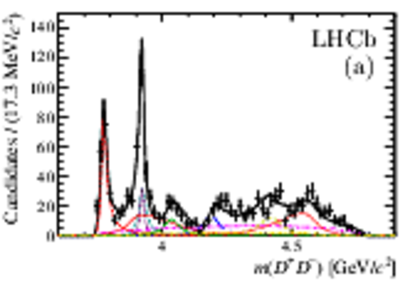
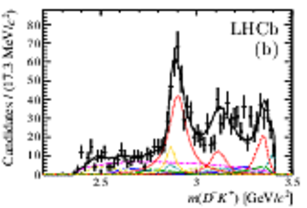
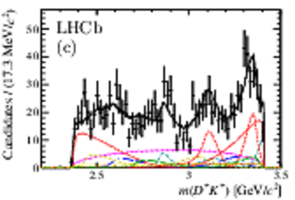
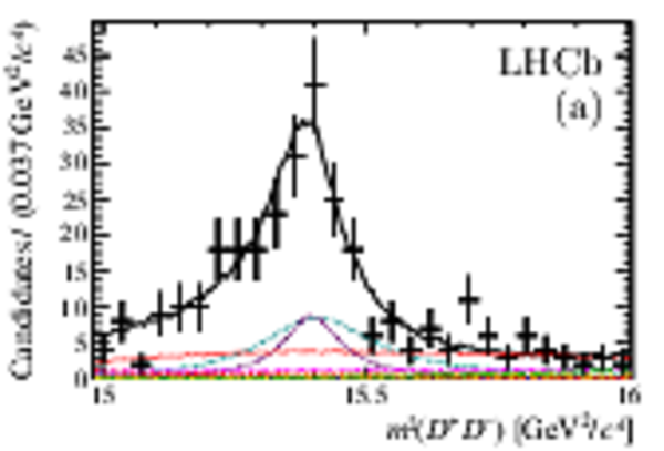
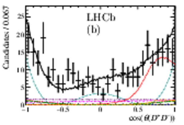
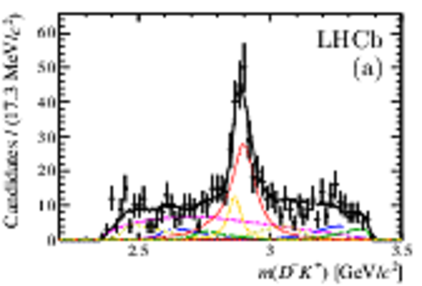
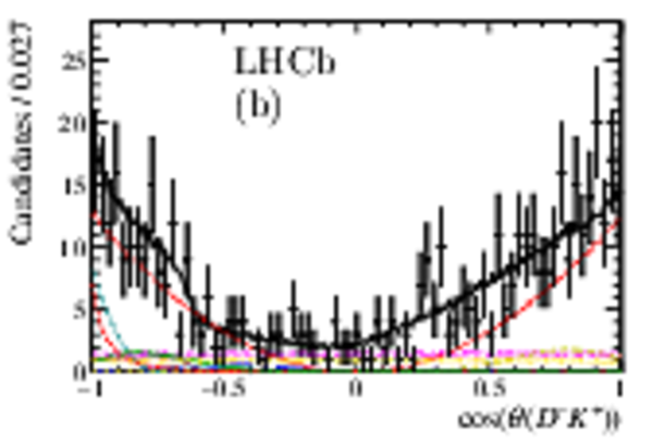
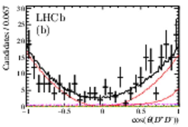
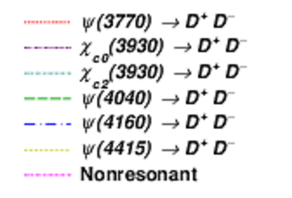
Comparisons of the invariant-mass distributions of $ B ^+ \rightarrow D ^+ D ^- K ^+ $ candidates in data to the fit projection of the baseline model. The total fit function and contributions from individual components are shown as detailed in the legend.	fig10a.pdf [131 KiB] HiDef png [410 KiB] Thumbnail [355 KiB] *.C file
	fig10b.pdf [134 KiB] HiDef png [465 KiB] Thumbnail [411 KiB] *.C file
	fig10c.pdf [151 KiB] HiDef png [488 KiB] Thumbnail [447 KiB] *.C file
	fig10d.pdf [11 KiB] HiDef png [308 KiB] Thumbnail [333 KiB] *.C file
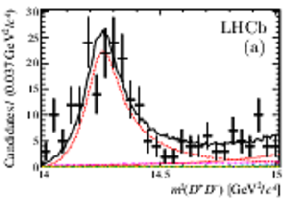
Comparison of the data and fit projection in the $\chi_{cJ}(3930)$ region, shown for the (a) $ D ^+ D ^- $ invariant-mass squared and (b) helicity angle. The different components are shown as indicated in the legend of Fig. ???.	fig11a.pdf [97 KiB] HiDef png [434 KiB] Thumbnail [384 KiB] *.C file
	fig11b.pdf [91 KiB] HiDef png [441 KiB] Thumbnail [406 KiB] *.C file
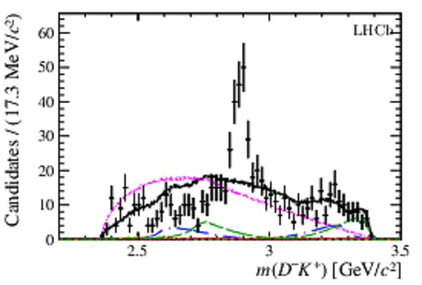
Comparison of data and the fit projection of the baseline model, for (a) the $ D ^- K ^+ $ invariant-mass distribution requiring $m( D ^+ D ^- )>4\text{ Ge V /}c^2 $ to suppress reflections from charmonium resonances and (b) helicity angle in the region $2.75\text{ Ge V /}c^2 <m( D ^- K ^+ )<3.05\text{ Ge V /}c^2 $. The different components are shown as indicated in the legend of Fig. ???.	fig12a.pdf [139 KiB] HiDef png [408 KiB] Thumbnail [379 KiB] *.C file
	fig12b.pdf [235 KiB] HiDef png [457 KiB] Thumbnail [411 KiB] *.C file
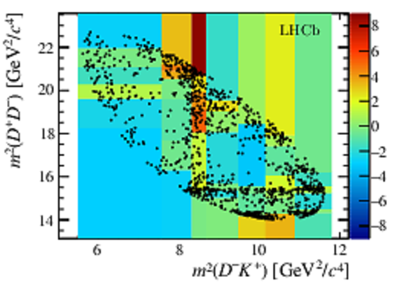
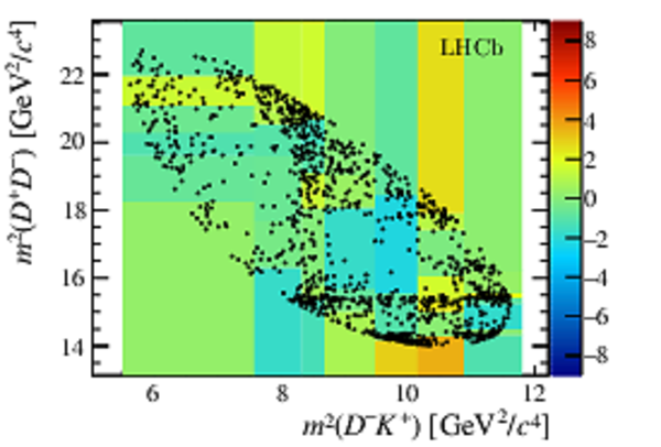
Normalised residual between the data and the baseline model including $ D ^- K ^+ $ resonances, shown across the Dalitz plot with a minimum of 20 entries in each bin.	fig13.pdf [105 KiB] HiDef png [569 KiB] Thumbnail [460 KiB] *.C file
Comparison of the data and fit projection in the region of the $\psi(3770)$ states, shown for the $ D ^+ D ^- $ (left) invariant-mass squared and (right) helicity angle. The different components are shown as indicated in the legend of Fig. ???.	fig14a.pdf [89 KiB] HiDef png [394 KiB] Thumbnail [393 KiB] *.C file
	fig14b.pdf [100 KiB] HiDef png [363 KiB] Thumbnail [360 KiB] *.C file
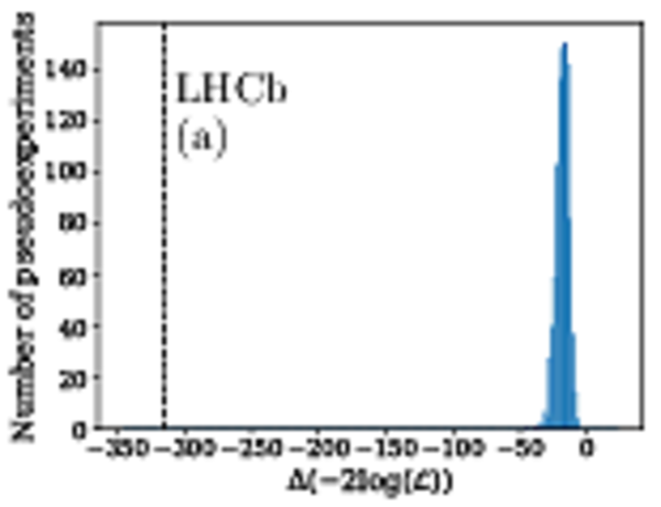
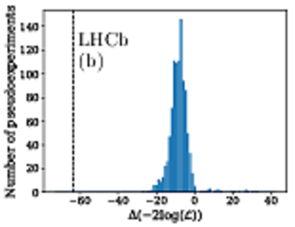
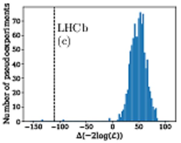
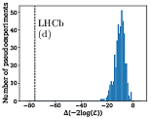
Distributions of the test-statistic $t$ in ensembles of pseudoexperiments generated according to various hypotheses and compared to values found in data (indicated by dashed vertical lines). In (a), the $H_0$ hypothesis is a model fit to data without $ D ^- K ^+ $ resonances. In (b), (c) and (d) plots, the $H_0$ hypothesis assumes a single $\chi_{cJ}(3930)$ state, which has spin-0, spin-1 and spin-2, respectively.	fig15a.pdf [24 KiB] HiDef png [215 KiB] Thumbnail [265 KiB] *.C file
	fig15b.pdf [22 KiB] HiDef png [213 KiB] Thumbnail [258 KiB] *.C file
	fig15c.pdf [23 KiB] HiDef png [219 KiB] Thumbnail [282 KiB] *.C file
	fig15d.pdf [23 KiB] HiDef png [195 KiB] Thumbnail [261 KiB] *.C file
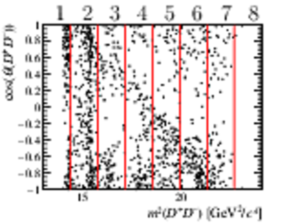
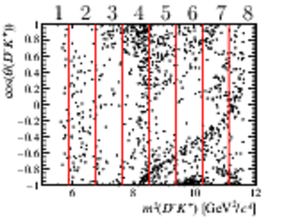
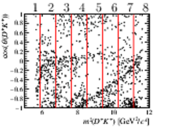
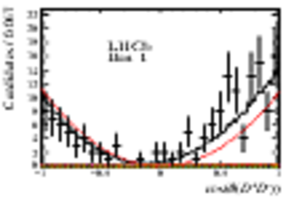
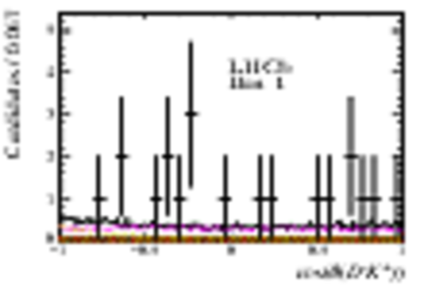
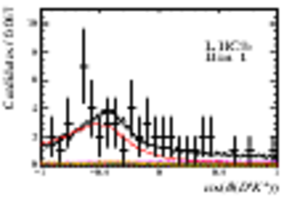
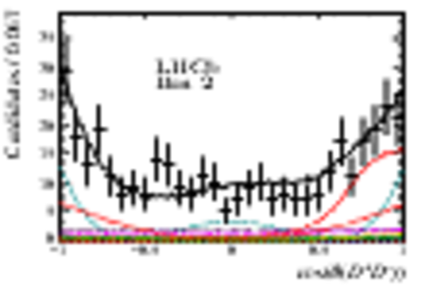
Division of the square Dalitz plot in slices of invariant mass squared. The binning is used for (top left) the $\cos\left(\theta( D ^+ D ^- )\right)$ distribution, (top right) the $\cos\left(\theta( D ^- K ^+ )\right)$ distribution, and (lower) the $\cos\left(\theta( D ^+ K ^+ )\right)$ distribution.	fig16a.pdf [59 KiB] HiDef png [533 KiB] Thumbnail [591 KiB] *.C file
	fig16b.pdf [59 KiB] HiDef png [535 KiB] Thumbnail [612 KiB] *.C file
	fig16c.pdf [59 KiB] HiDef png [538 KiB] Thumbnail [621 KiB] *.C file
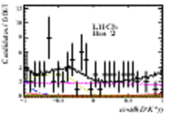
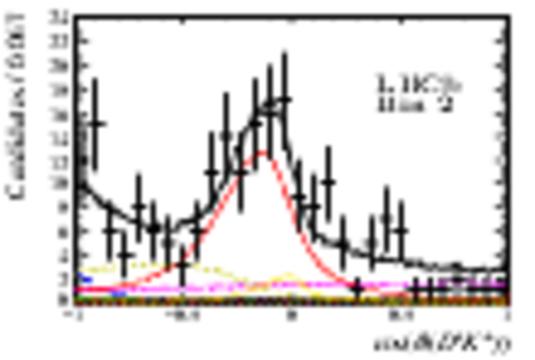
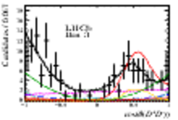
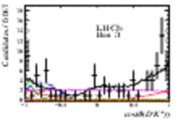
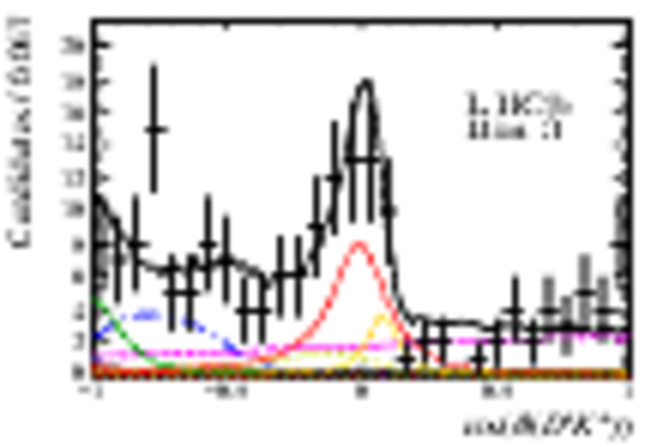
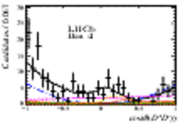
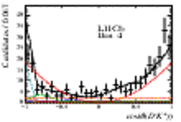
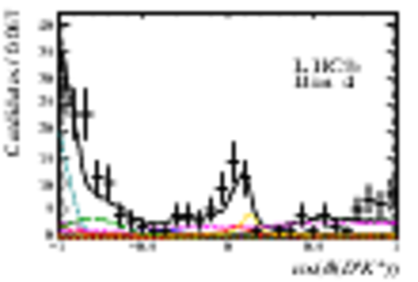
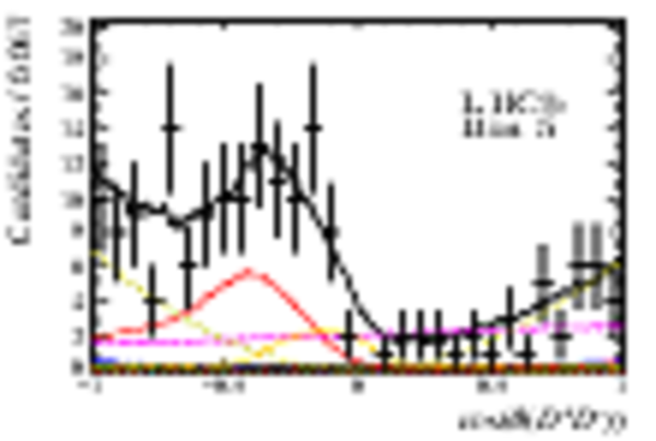
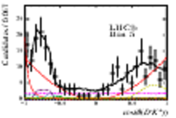
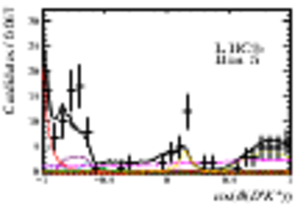
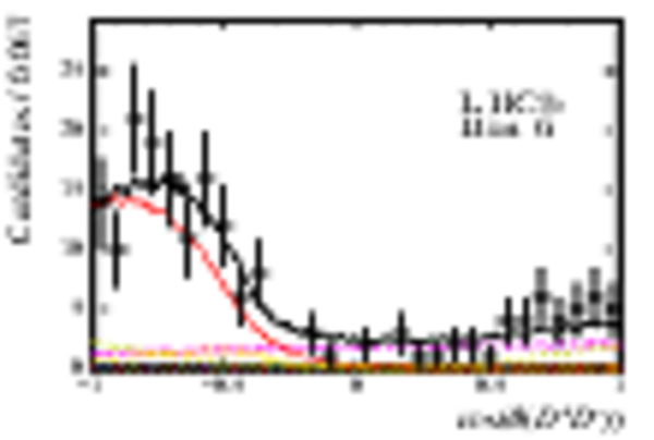
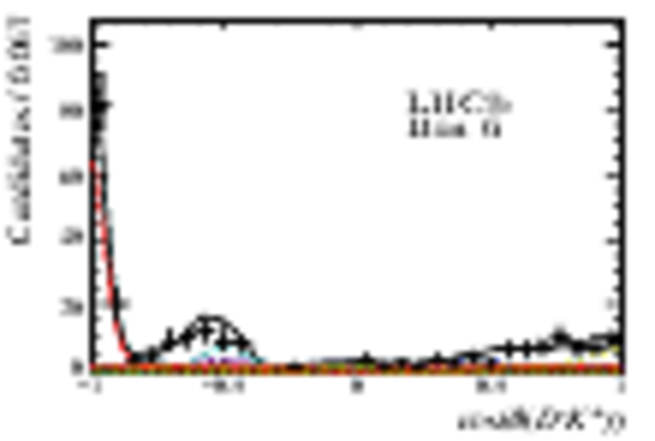
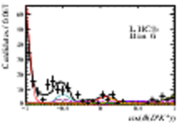
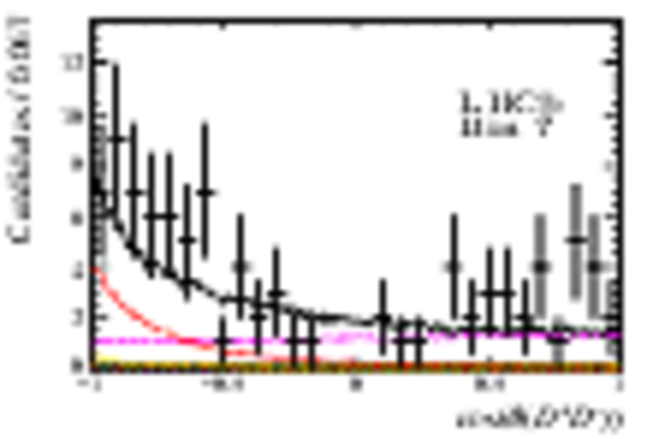
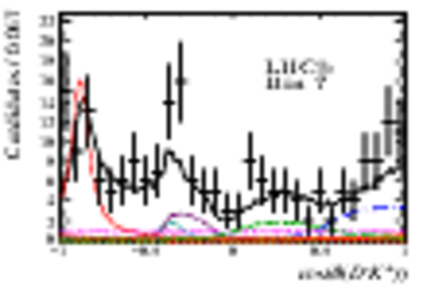
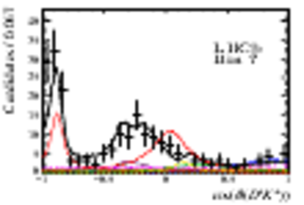
Helicity-angle distributions divided according to the binning scheme shown in Fig. ??? (bins 1-4). The different components are shown as indicated in the legend of Fig. ???.	fig17a.pdf [105 KiB] HiDef png [481 KiB] Thumbnail [411 KiB] *.C file
	fig17b.pdf [127 KiB] HiDef png [409 KiB] Thumbnail [344 KiB] *.C file
	fig17c.pdf [117 KiB] HiDef png [446 KiB] Thumbnail [378 KiB] *.C file
	fig17d.pdf [91 KiB] HiDef png [599 KiB] Thumbnail [456 KiB] *.C file
	fig17e.pdf [106 KiB] HiDef png [505 KiB] Thumbnail [427 KiB] *.C file
	fig17f.pdf [91 KiB] HiDef png [579 KiB] Thumbnail [467 KiB] *.C file
	fig17g.pdf [86 KiB] HiDef png [628 KiB] Thumbnail [463 KiB] *.C file
	fig17h.pdf [95 KiB] HiDef png [529 KiB] Thumbnail [410 KiB] *.C file
	fig17i.pdf [86 KiB] HiDef png [583 KiB] Thumbnail [465 KiB] *.C file
	fig17j.pdf [88 KiB] HiDef png [492 KiB] Thumbnail [386 KiB] *.C file
	fig17k.pdf [94 KiB] HiDef png [560 KiB] Thumbnail [420 KiB] *.C file
	fig17l.pdf [83 KiB] HiDef png [510 KiB] Thumbnail [386 KiB] *.C file
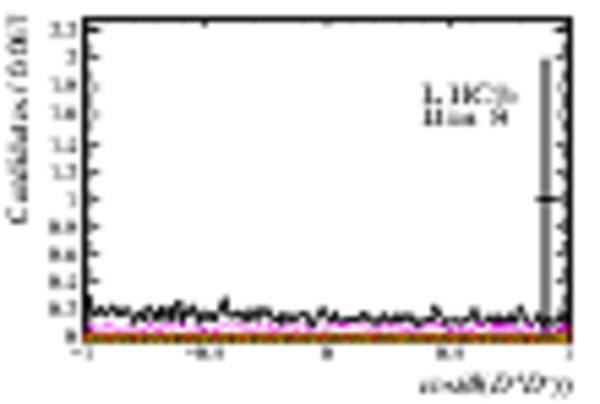
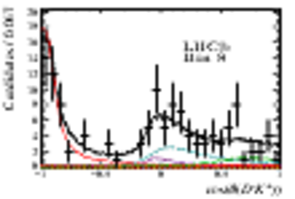
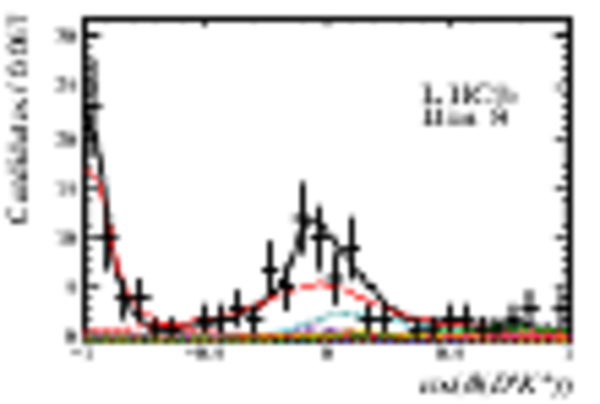
Helicity-angle distributions divided according to the binning scheme shown in Fig. ??? (bins 5-8). The different components are shown as indicated in the legend of Fig. ???.	fig18a.pdf [89 KiB] HiDef png [564 KiB] Thumbnail [454 KiB] *.C file
	fig18b.pdf [92 KiB] HiDef png [564 KiB] Thumbnail [436 KiB] *.C file
	fig18c.pdf [86 KiB] HiDef png [496 KiB] Thumbnail [376 KiB] *.C file
	fig18d.pdf [94 KiB] HiDef png [476 KiB] Thumbnail [380 KiB] *.C file
	fig18e.pdf [86 KiB] HiDef png [403 KiB] Thumbnail [305 KiB] *.C file
	fig18f.pdf [77 KiB] HiDef png [480 KiB] Thumbnail [341 KiB] *.C file
	fig18g.pdf [104 KiB] HiDef png [459 KiB] Thumbnail [414 KiB] *.C file
	fig18h.pdf [93 KiB] HiDef png [607 KiB] Thumbnail [469 KiB] *.C file
	fig18i.pdf [79 KiB] HiDef png [552 KiB] Thumbnail [392 KiB] *.C file
	fig18j.pdf [109 KiB] HiDef png [457 KiB] Thumbnail [345 KiB] *.C file
	fig18k.pdf [103 KiB] HiDef png [546 KiB] Thumbnail [430 KiB] *.C file
	fig18l.pdf [95 KiB] HiDef png [517 KiB] Thumbnail [371 KiB] *.C file
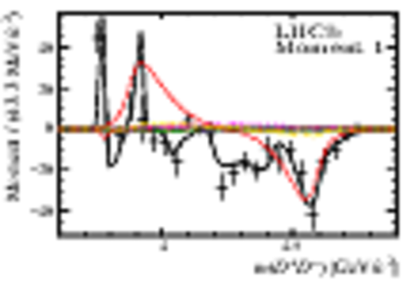
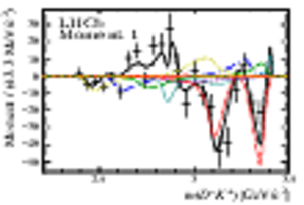
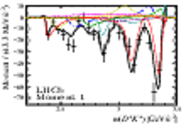
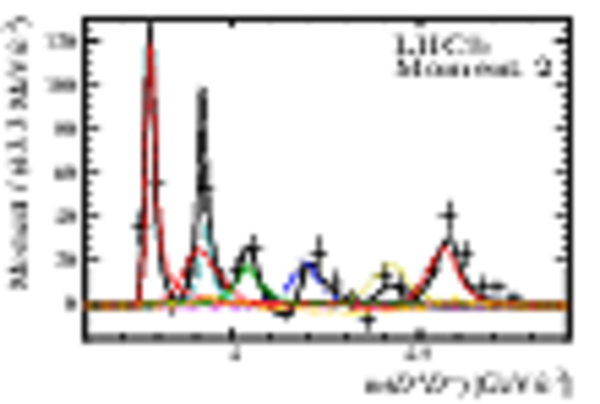
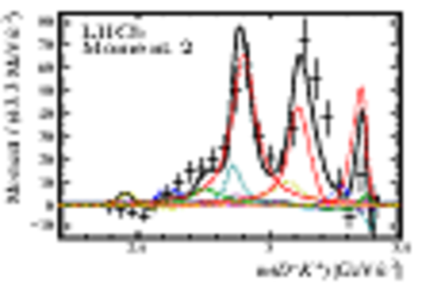
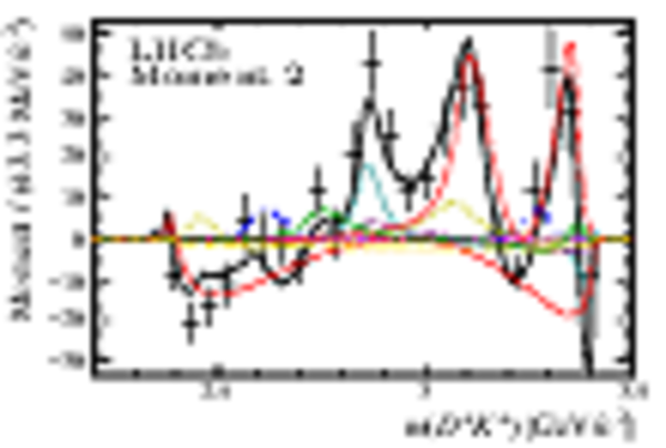
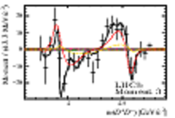
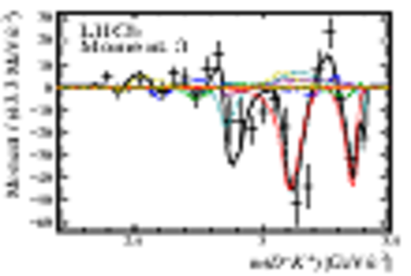
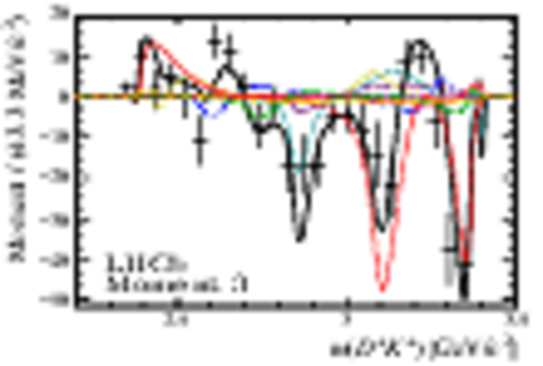
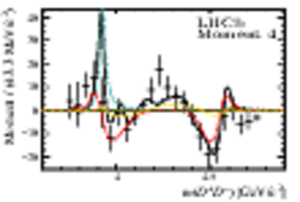
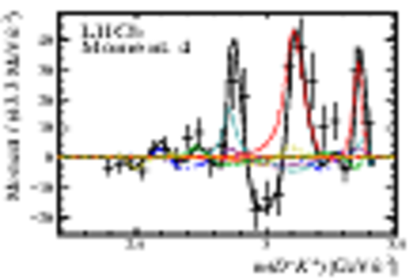
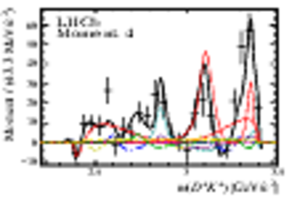
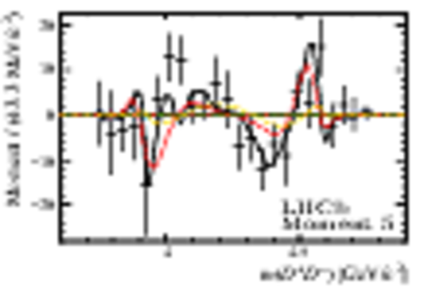
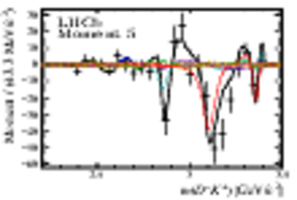
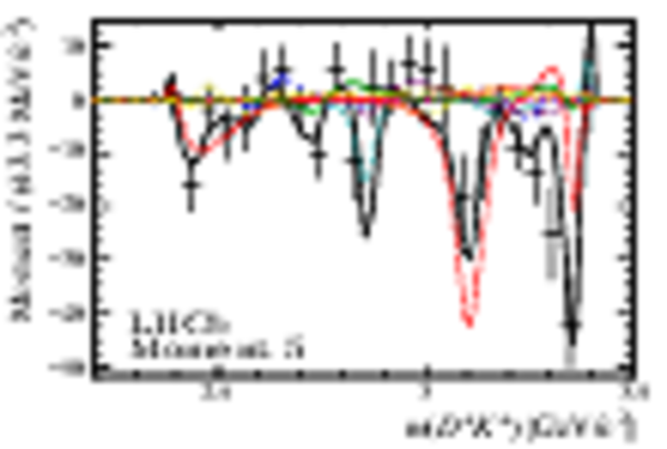
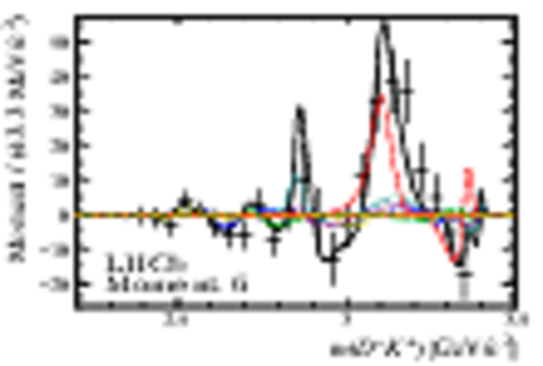
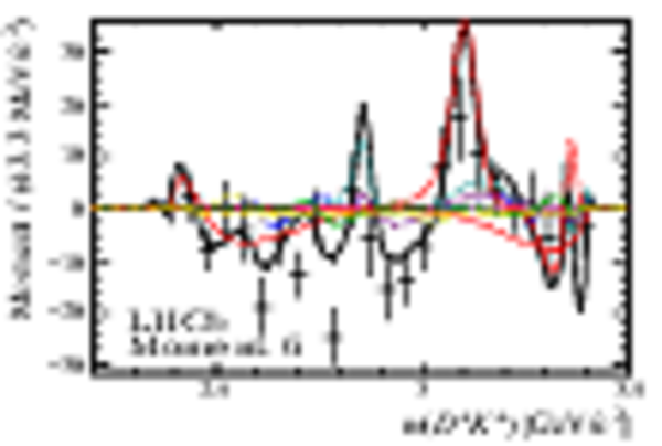
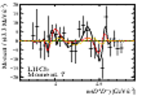
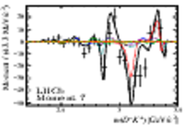
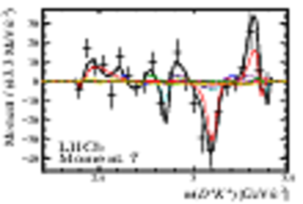
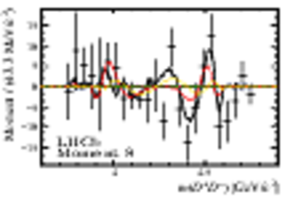
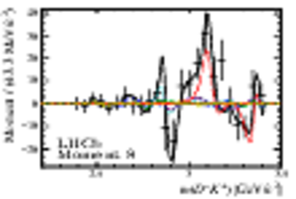
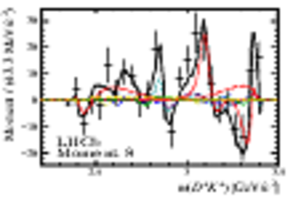
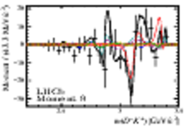
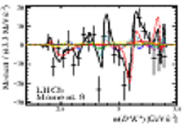
Projections of moments 1--5 of each pair of final-state particles in the $ B ^+ \rightarrow D ^+ D ^- K ^+ $ Dalitz plot. As usual, data points are shown in black and the total, and individual components' PDFs are overlaid. The different components are shown as indicated in the legend of Fig. ???.	fig19a.pdf [66 KiB] HiDef png [504 KiB] Thumbnail [421 KiB] *.C file
	fig19b.pdf [58 KiB] HiDef png [646 KiB] Thumbnail [474 KiB] *.C file
	fig19c.pdf [46 KiB] HiDef png [720 KiB] Thumbnail [513 KiB] *.C file
	fig19d.pdf [54 KiB] HiDef png [592 KiB] Thumbnail [430 KiB] *.C file
	fig19e.pdf [53 KiB] HiDef png [711 KiB] Thumbnail [499 KiB] *.C file
	fig19f.pdf [51 KiB] HiDef png [737 KiB] Thumbnail [515 KiB] *.C file
	fig19g.pdf [73 KiB] HiDef png [534 KiB] Thumbnail [446 KiB] *.C file
	fig19h.pdf [58 KiB] HiDef png [639 KiB] Thumbnail [460 KiB] *.C file
	fig19i.pdf [52 KiB] HiDef png [727 KiB] Thumbnail [512 KiB] *.C file
	fig19j.pdf [69 KiB] HiDef png [554 KiB] Thumbnail [439 KiB] *.C file
	fig19k.pdf [61 KiB] HiDef png [643 KiB] Thumbnail [469 KiB] *.C file
	fig19l.pdf [53 KiB] HiDef png [702 KiB] Thumbnail [498 KiB] *.C file
	fig19m.pdf [74 KiB] HiDef png [495 KiB] Thumbnail [432 KiB] *.C file
	fig19n.pdf [62 KiB] HiDef png [591 KiB] Thumbnail [442 KiB] *.C file
	fig19o.pdf [54 KiB] HiDef png [679 KiB] Thumbnail [494 KiB] *.C file
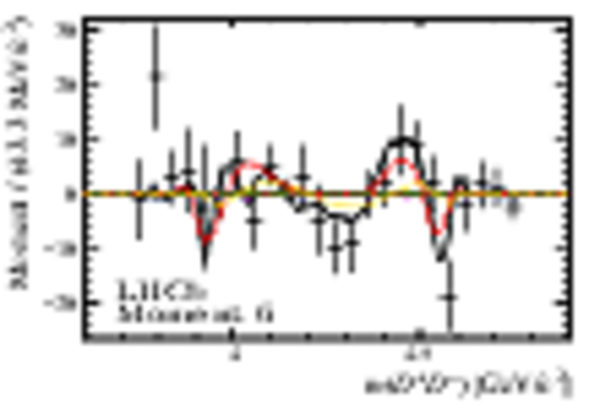
Projections of moments 6--9 of each pair of final-state particles in the $ B ^+ \rightarrow D ^+ D ^- K ^+ $ Dalitz plot. As usual, data points are shown in black and the total, and individual components' PDFs are overlaid. The different components are shown as indicated in the legend of Fig. ???.	fig20a.pdf [75 KiB] HiDef png [474 KiB] Thumbnail [412 KiB] *.C file
	fig20b.pdf [64 KiB] HiDef png [581 KiB] Thumbnail [438 KiB] *.C file
	fig20c.pdf [54 KiB] HiDef png [666 KiB] Thumbnail [472 KiB] *.C file
	fig20d.pdf [78 KiB] HiDef png [518 KiB] Thumbnail [451 KiB] *.C file
	fig20e.pdf [64 KiB] HiDef png [579 KiB] Thumbnail [446 KiB] *.C file
	fig20f.pdf [57 KiB] HiDef png [590 KiB] Thumbnail [444 KiB] *.C file
	fig20g.pdf [79 KiB] HiDef png [503 KiB] Thumbnail [447 KiB] *.C file
	fig20h.pdf [68 KiB] HiDef png [563 KiB] Thumbnail [435 KiB] *.C file
	fig20i.pdf [56 KiB] HiDef png [641 KiB] Thumbnail [485 KiB] *.C file
	fig20j.pdf [80 KiB] HiDef png [494 KiB] Thumbnail [446 KiB] *.C file
	fig20k.pdf [67 KiB] HiDef png [573 KiB] Thumbnail [456 KiB] *.C file
	fig20l.pdf [60 KiB] HiDef png [636 KiB] Thumbnail [485 KiB] *.C file
Animated gif made out of all figures.	PAPER-2020-025.gif Thumbnail

Tables and captions

Signal and background component yields obtained from the simultaneous fit to the Run 1 and Run 2 data-taking years.	Table_1.pdf [38 KiB] HiDef png [96 KiB] Thumbnail [45 KiB] tex code
Fitted values of shape parameters of the DSCB and exponential PDFs used to model signal and background, respectively, in the simultaneous fit to Run 1 and Run 2 data.	Table_2.pdf [62 KiB] HiDef png [75 KiB] Thumbnail [37 KiB] tex code
Components which may appear in the $ D ^+ D ^- $ spectrum of $ B ^+ \rightarrow D ^+ D ^- K ^+ $ decays, and their properties as given by the Particle Data Group (PDG) \cite{PDG2019}. For the $\psi(3770)$ mass and the mass/width of both the $\chi_{c2}(3930)$ and $X(3842)$, the values in Ref. \cite{LHCb-PAPER-2019-005} are used.	Table_3.pdf [70 KiB] HiDef png [67 KiB] Thumbnail [31 KiB] tex code
Magnitude and phase of the complex coefficients in the amplitude model, together with fit fractions for each component. The quantities are reported after correction for fit biases (see Sec. ???). The first uncertainty is statistical and the second is the sum in quadrature of all systematic uncertainties.	Table_4.pdf [71 KiB] HiDef png [115 KiB] Thumbnail [54 KiB] tex code
Lineshape parameters for the $\chi_{c0,2}(3930)$ and $X_{0,1}(2900)$ resonances determined from the fit. The first uncertainty is statistical and the second is the sum in quadrature of all systematic uncertainties.	Table_5.pdf [61 KiB] HiDef png [65 KiB] Thumbnail [30 KiB] tex code
Interference fit fractions (%) obtained from the results of the amplitude fit with the baseline model. Uncertainties are statistical and systematic, respectively. Absent entries correspond to pairs of resonances that do not interfere, because they either inhabit separate regions of phase space or belong to different partial waves in the same two-body combination.	Table_6.pdf [60 KiB] HiDef png [43 KiB] Thumbnail [16 KiB] tex code
Model variations and the associated negative log-likelihood (NLL) and $\chi^2$ values.	Table_7.pdf [71 KiB] HiDef png [131 KiB] Thumbnail [57 KiB] tex code
Systematic uncertainties on the complex coefficients and fit fractions of each component of the amplitude model: mass-fit signal shape (1), size of simulated sample for efficiencies (2), hardware trigger modelling (3), modelling: parent Blatt--Weisskopf radius (4), modelling: charmonia Blatt--Weisskopf radius (5), modelling: $ D ^- K ^+ $ resonances' Blatt--Weisskopf radius (6), model composition: S wave (7), model composition: P wave (8).	Table_8.pdf [65 KiB] HiDef png [190 KiB] Thumbnail [61 KiB] tex code
Systematic uncertainties on the masses ( $\text{Ge V /}c^2$ ) and widths ( $\text{Ge V}$ ) of the $\chi_{c0,2}(3930)$ and $X_{0,1}(2900)$ resonances: mass-fit signal shape (1), size of simulated sample for efficiencies (2), hardware trigger modelling (3), modelling: parent Blatt--Weisskopf radius (4), modelling: charmonia Blatt--Weisskopf radius (5), modelling: $ D ^- K ^+ $ resonances' Blatt--Weisskopf radius (6), model composition: S wave (7), model composition: P wave (8).	Table_9.pdf [62 KiB] HiDef png [71 KiB] Thumbnail [22 KiB] tex code