Leading-order Feynman diagrams for (left) $ B ^0_ s $ and (right) $\overline{ B } {}^0_ s $ decays to the $D_s^- K^+ \pi ^+ \pi ^- $ final state, where the $\pi ^+ \pi ^- $ subsystem exemplarily hadronises in conjunction with the kaon.

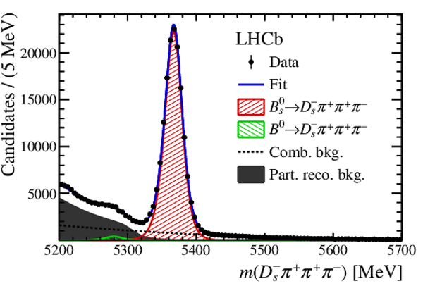
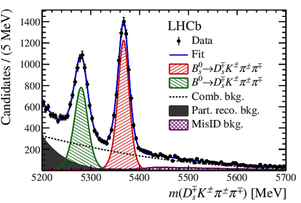
Invariant mass distribution of selected (left) $ B ^0_ s \rightarrow D ^-_ s \pi ^+ \pi ^+ \pi ^- $ and (right) $ B ^0_ s \rightarrow D ^{\mp}_ s K ^\pm \pi ^\pm \pi ^\mp $ candidates with fit projections overlaid.

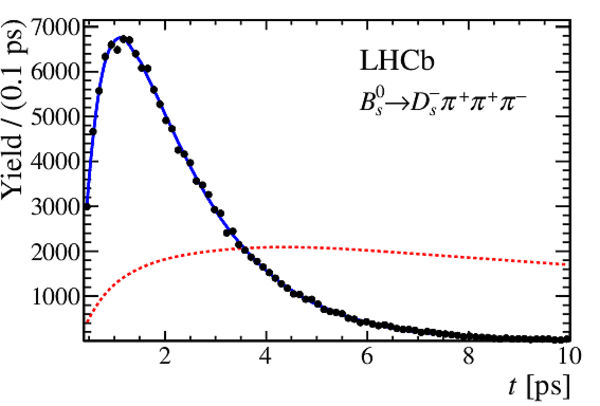
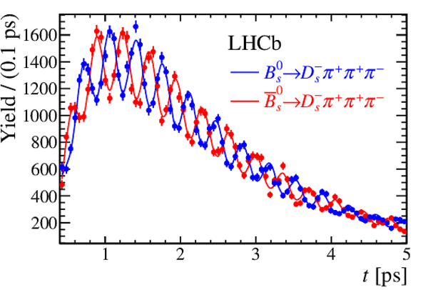
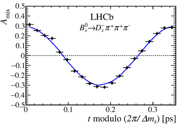
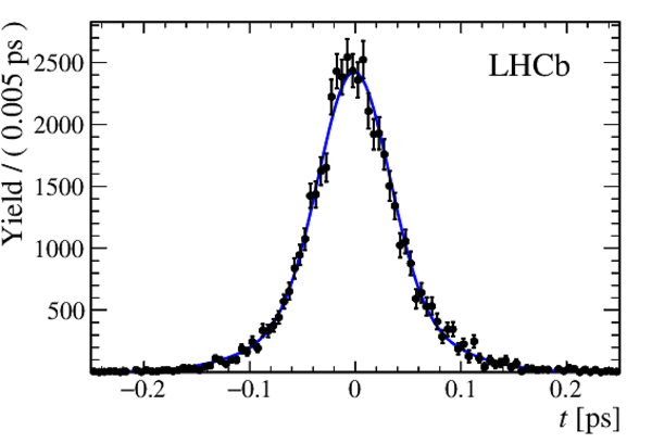
Background-subtracted decay-time distribution of (top) all and (bottom left) tagged $ B ^0_ s \rightarrow D ^-_ s \pi ^+ \pi ^+ \pi ^- $ candidates as well as (bottom right) the dilution-weighted mixing asymmetry folded into one oscillation period along with the fit projections (solid lines). The decay-time acceptance (top) is overlaid in an arbitrary scale (dashed line).

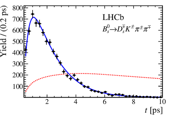
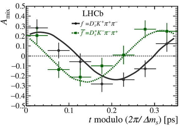
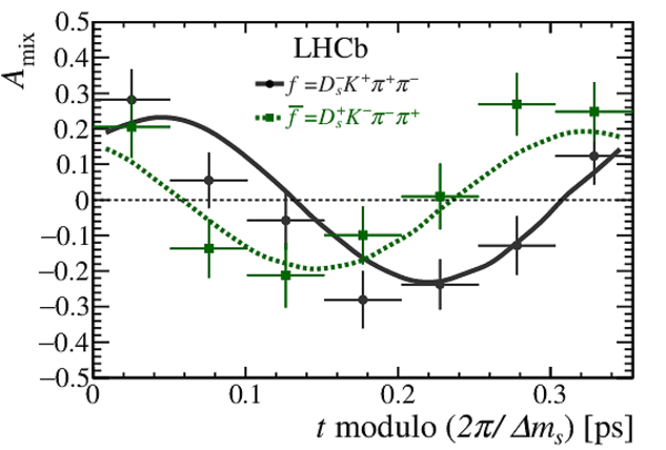
Decay-time distribution of (left) background-subtracted $ B ^0_ s \rightarrow D ^{\mp}_ s K ^\pm \pi ^\pm \pi ^\mp $ candidates and (right) dilution-weighted mixing asymmetry along with the model-independent fit projections (lines). The decay-time acceptance (left) is overlaid in an arbitrary scale (dashed line).

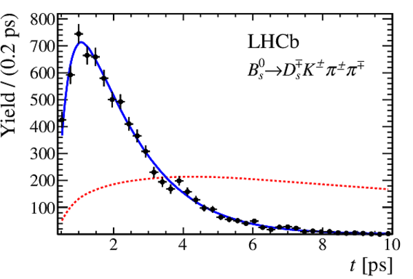
Decay-time distribution of (left) background-subtracted $ B ^0_ s \rightarrow D ^{\mp}_ s K ^\pm \pi ^\pm \pi ^\mp $ candidates and (right) dilution-weighted mixing asymmetry along with the model-dependent fit projections (lines). The decay-time acceptance (left) is overlaid in an arbitrary scale (dashed line).

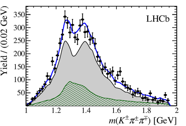
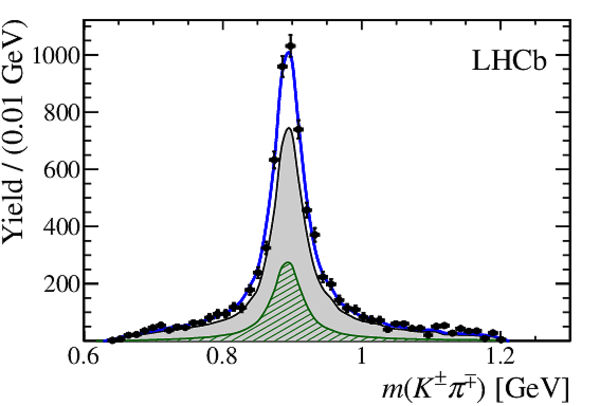
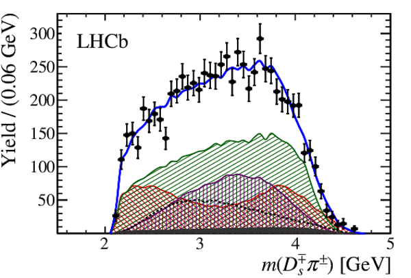
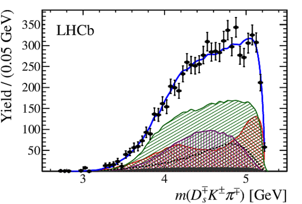
Invariant-mass distribution of background-subtracted $ B ^0_ s \rightarrow D ^{\mp}_ s K ^\pm \pi ^\pm \pi ^\mp $ candidates (data points) and fit projections (blue solid line). Contributions from $b\rightarrow c$ and $b\rightarrow u$ decay amplitudes are overlaid.

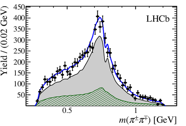
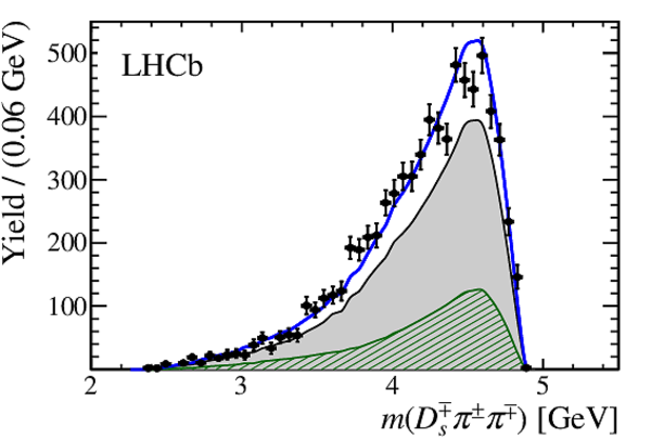
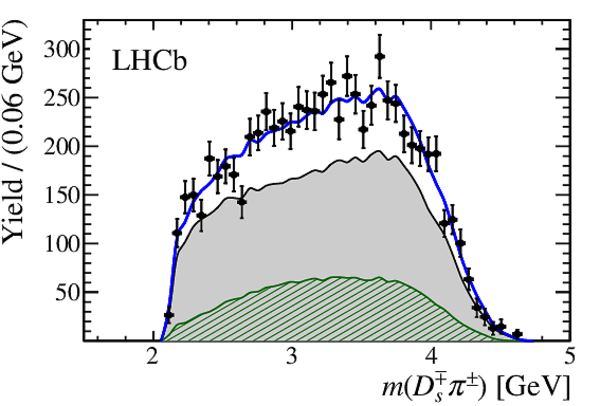
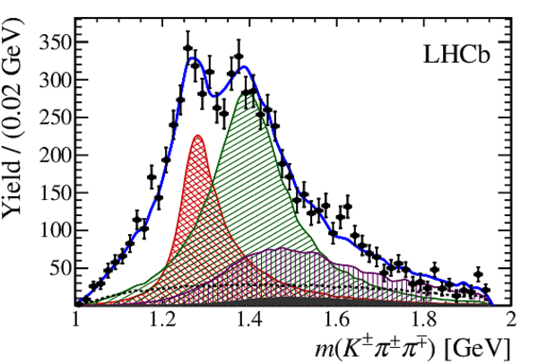
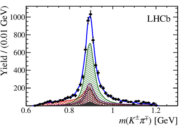
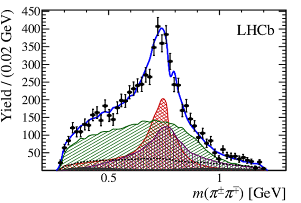
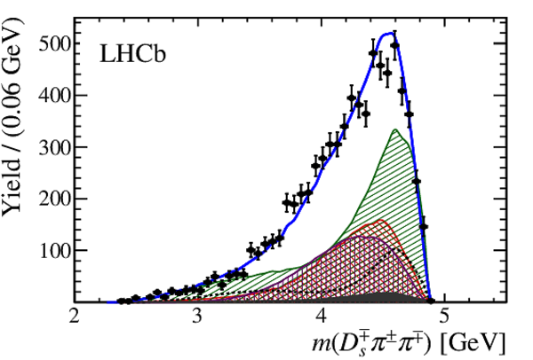
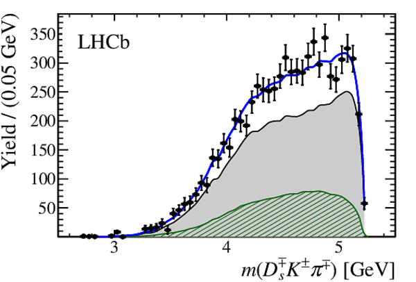
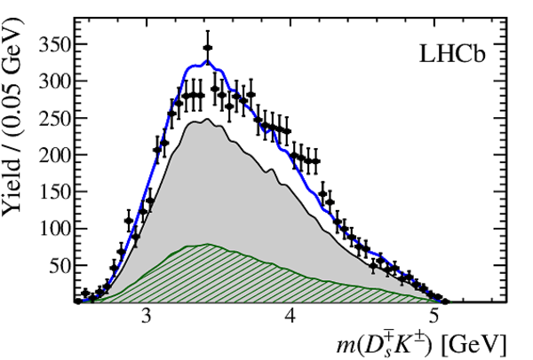
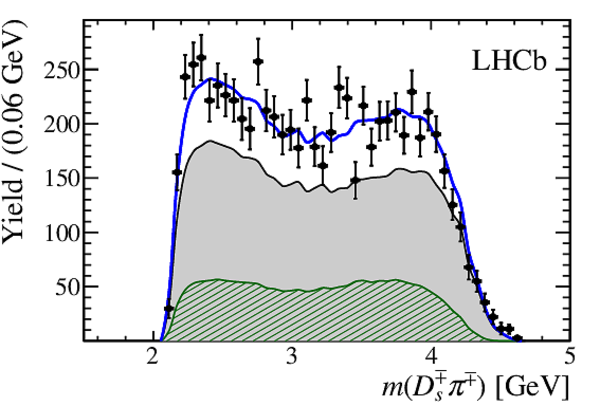
Invariant-mass distribution of background-subtracted $ B ^0_ s \rightarrow D ^{\mp}_ s K ^\pm \pi ^\pm \pi ^\mp $ candidates (data points) and fit projections (blue solid line). Incoherent contributions from intermediate-state components are overlaid.

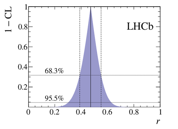
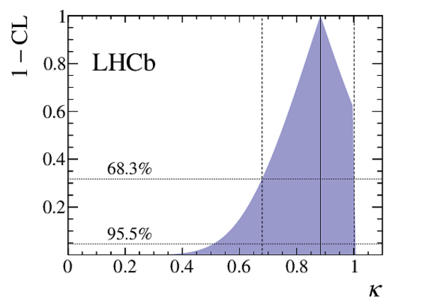
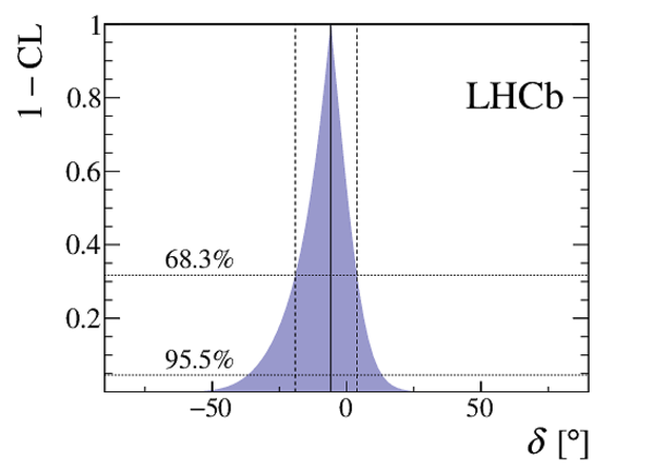
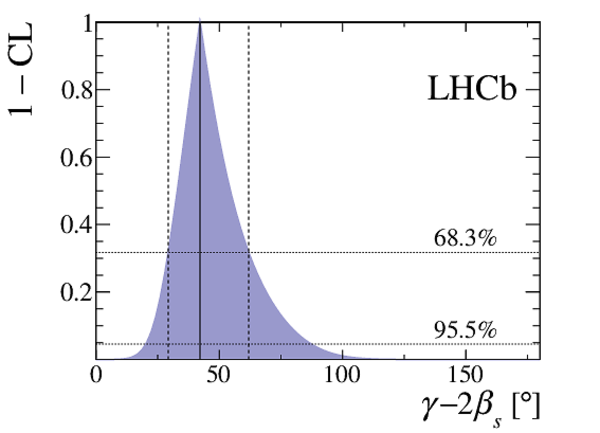
The 1$-$CL contours for the physical observables $r,\kappa,\delta$ and $\gamma-2\beta_s$ obtained with the model-independent fit.

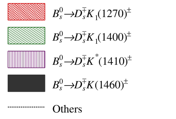
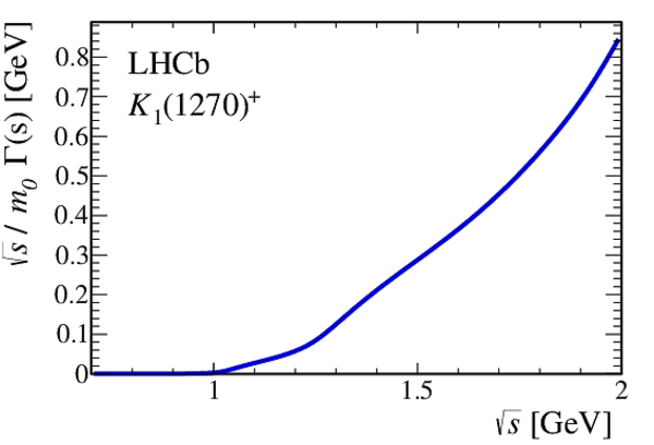
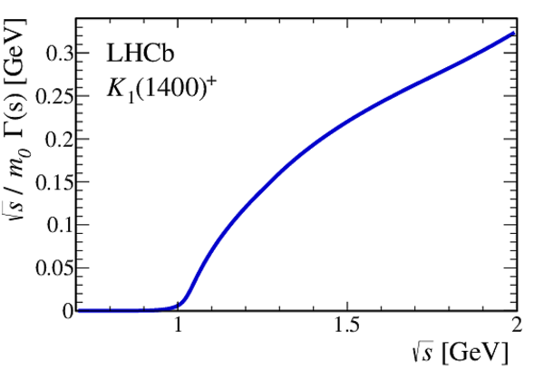
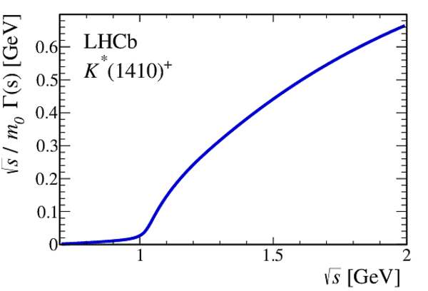
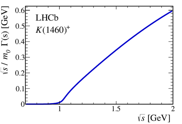
Running width distributions of the three-body resonances included in the baseline model for $ B ^0_ s \rightarrow D ^{\mp}_ s K ^\pm \pi ^\pm \pi ^\mp $ decays: (top left) $K_1(1270)^+$, (top right) $K_1(1400)^+$, (bottom left) $K^*(1410)^+$ and (bottom right) $K(1460)^+$.

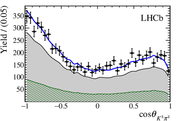
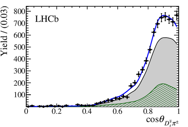
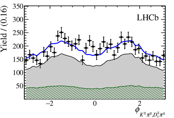
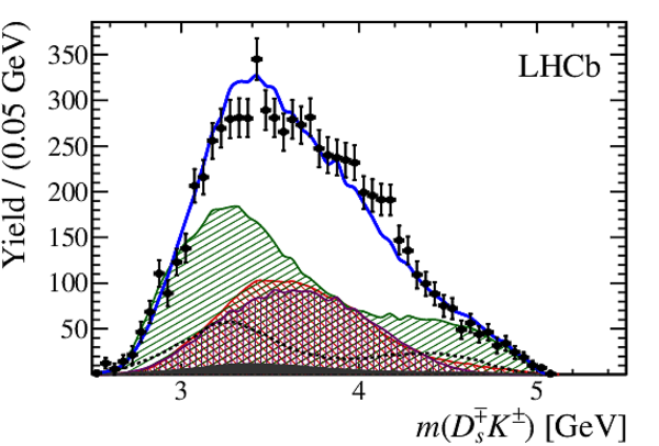
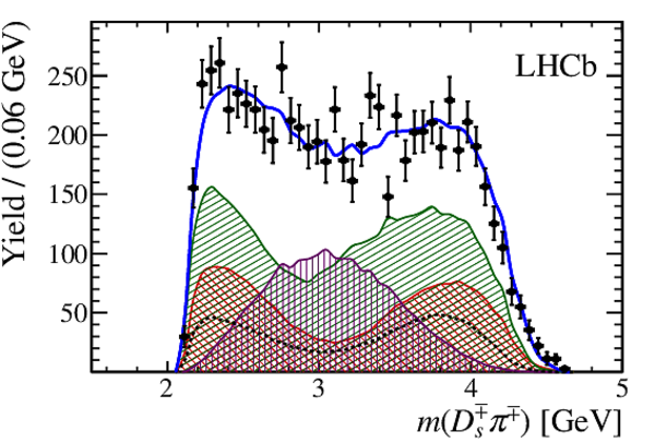
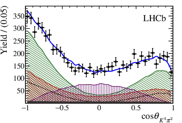
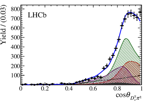
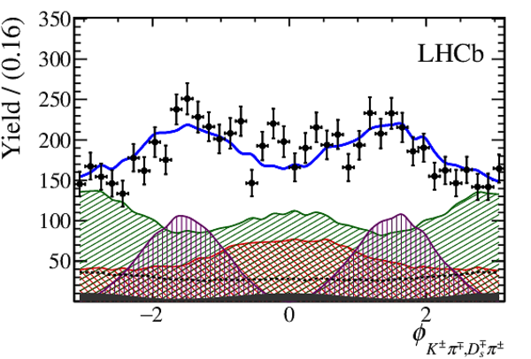
Invariant-mass and angular distributions of background-subtracted $ B ^0_ s \rightarrow D ^{\mp}_ s K ^\pm \pi ^\pm \pi ^\mp $ candidates (data points) and fit projections (blue solid line). Contributions from $b\rightarrow c$ and $b\rightarrow u$ decay amplitudes are overlaid, colour coded as in Fig. ???.

Invariant-mass and angular distributions of background-subtracted $ B ^0_ s \rightarrow D ^{\mp}_ s K ^\pm \pi ^\pm \pi ^\mp $ candidates (data points) and fit projections (blue solid line). Incoherent contributions from intermediate-state components are overlaid, colour coded as in Fig. ???.

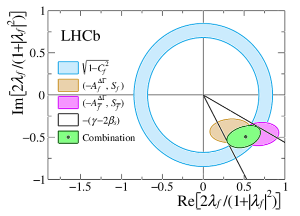
Visualisation of how the $ C P$ coefficients contribute towards the overall constraint on the weak phase, $\gamma - 2\beta_s$. The difference between the phase of $(-A_f^{\Delta\Gamma},S_f)$ and $(-A_{\bar{f}}^{\Delta\Gamma},S_{\bar{f}})$ is proportional to the strong phase $\delta$, which is close to $0 ^{\circ} $ and thus not indicated in the figure.

Animated gif made out of all figures.

The flavour-tagging performance for only OS-tagged, only SS-tagged and both OS- and SS-tagged $ B ^0_ s \rightarrow D ^-_ s \pi ^+ \pi ^+ \pi ^- $ signal candidates.

$ C P$ coefficients determined from the phase-space fit to the $ B ^0_ s \rightarrow D ^{\mp}_ s K ^\pm \pi ^\pm \pi ^\mp $ decay-time distribution. The uncertainties are statistical and systematic (discussed in Sec. ???).

Decay fractions of the intermediate-state amplitudes contributing to decays via $b \rightarrow c$ and $b \rightarrow u$ quark-level transitions. The uncertainties are statistical, systematic and due to alternative amplitude models considered.

Systematic uncertainties on the $ B ^0_ s $ mixing frequency determined from the fit to $ B ^0_ s \rightarrow D ^-_ s \pi ^+ \pi ^+ \pi ^- $ signal candidates and on the fit parameters of the phase-space integrated fit to $ B ^0_ s \rightarrow D ^{\mp}_ s K ^\pm \pi ^\pm \pi ^\mp $ signal candidates in units of the statistical standard deviations.

Systematic uncertainties on the physical observables and resonance parameters determined from the full time-dependent amplitude fit to $ B ^0_ s \rightarrow D ^{\mp}_ s K ^\pm \pi ^\pm \pi ^\mp $ data in units of the statistical standard deviations. The systematic uncertainties for the amplitude coefficients are given in Table ???.

Parameters determined from the model-independent and model-dependent fits to the $ B ^0_ s \rightarrow D ^{\mp}_ s K ^\pm \pi ^\pm \pi ^\mp $ signal candidates. The uncertainties are statistical, systematic and (if applicable) due to alternative amplitude models considered. The angles are given modulo $180 ^{\circ} $.

Parameters of the resonances included in the $ B ^0_ s \rightarrow D ^{\mp}_ s K ^\pm \pi ^\pm \pi ^\mp $ baseline model.

Intermediate-state components considered for the $ B ^0_ s \rightarrow D ^{\mp}_ s K ^\pm \pi ^\pm \pi ^\mp $ LASSO model building procedure. The letters in square brackets and subscripts refer to the relative orbital angular momentum of the decay products in spectroscopic notation. If no angular momentum is specified, the lowest angular momentum state compatible with angular momentum conservation and, where appropriate, parity conservation, is used.

Moduli and phases of the amplitude coefficients for decays via $b \rightarrow c$ and $b \rightarrow u$ quark-level transitions. The uncertainties are statistical and systematic.

Moduli and phases of the amplitude coefficients for cascade decays. The amplitude coefficients are defined relative to the respective three-body production amplitude coefficients in Table ??? and are shared among $b \rightarrow c$ and $b \rightarrow u$ transitions. The uncertainties are statistical and systematic.

Systematic uncertainties on the fit parameters of the full time-dependent amplitude fit to $ B ^0_ s \rightarrow D ^{\mp}_ s K ^\pm \pi ^\pm \pi ^\mp $ data in units of the statistical standard deviations. The different contributions are: 1) fit bias, 2) background subtraction, 3) correlation of observables, 4) time acceptance, 5) resolution, 6) decay-time bias, 7) nuisance asymmetries, 8) $\Delta m_s$, 9) phase-space acceptance, 10) acceptance factorisation, 11) lineshape models, 12) masses and widths of resonances, 13) form factor.

Amplitude ratio and strong-phase difference for a given decay channel. The uncertainties are statistical and systematic.

Interference fractions (ordered by magnitude) of the $b\rightarrow c$ intermediate-state amplitudes included in the baseline model. Only the statistical uncertainties are given.

Interference fractions (ordered by magnitude) of the $b\rightarrow u$ intermediate-state amplitudes included in the baseline model. Only the statistical uncertainties are given.

Decay fractions in percent for several alternative amplitude models (Alt. 1 - Alt. 6). Resonance parameters and the observables $r, \kappa, \delta, \gamma - 2 \beta_s$ are also given.

Decay fractions in percent for several alternative amplitude models (Alt. 7 - Alt. 12). Resonance parameters and the observables $r, \kappa, \delta, \gamma - 2 \beta_s$ are also given.

Statistical correlation of the $ C P$ coefficients.

Supplementary material full pdf

This ZIP file contains supplemetary material for the publication LHCb-PAPER-2020-030. The files are: Supplementary.pdf : An overview of the extra figures *.pdf, *.png, *.eps, *.C : The figures in variuous formats