Angular Analysis of the $B^{+}\rightarrow K^{\ast+}\mu^{+}\mu^{-}$ Decay
[to restricted-access page]Information
LHCb-PAPER-2020-041
CERN-EP-2020-239
arXiv:2012.13241 [PDF]
(Submitted on 24 Dec 2020)
Phys. Rev. Lett.126 (2021) 161802
Inspire 1838196
Tools
Abstract
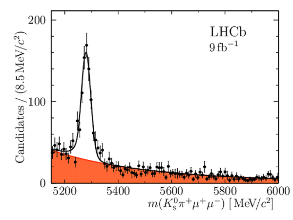
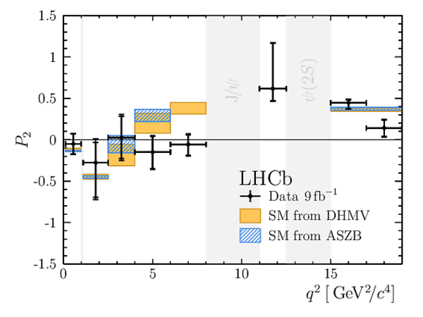
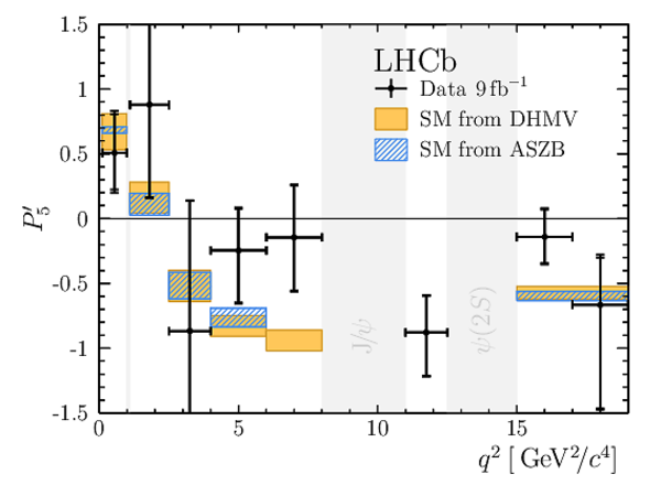
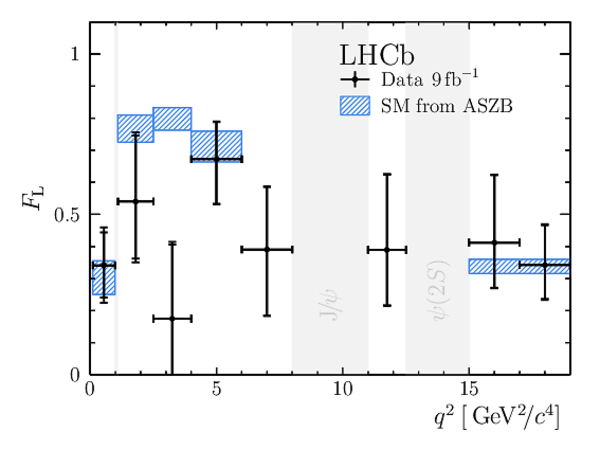
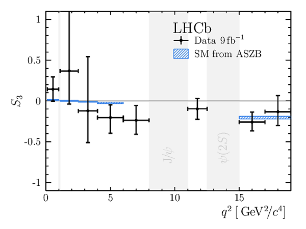
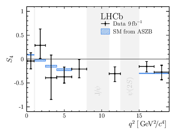
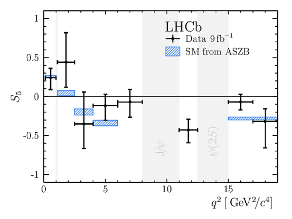
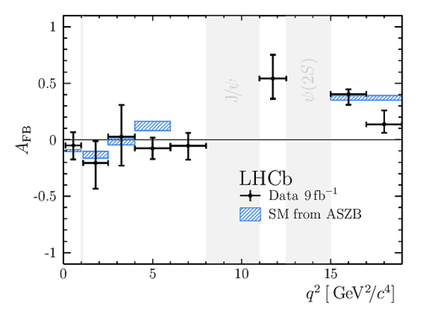
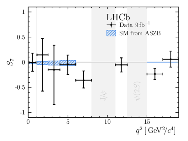
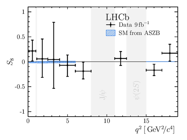
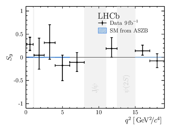
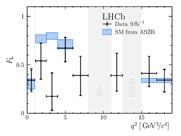
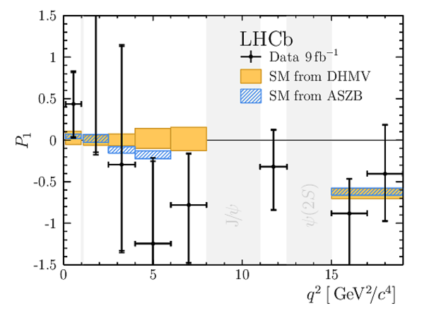
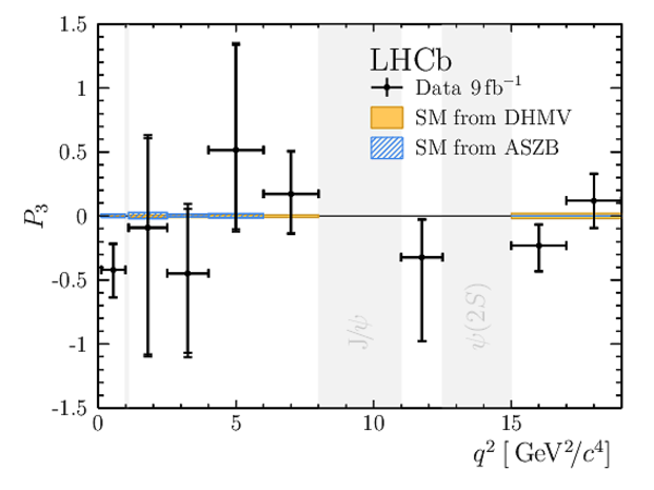
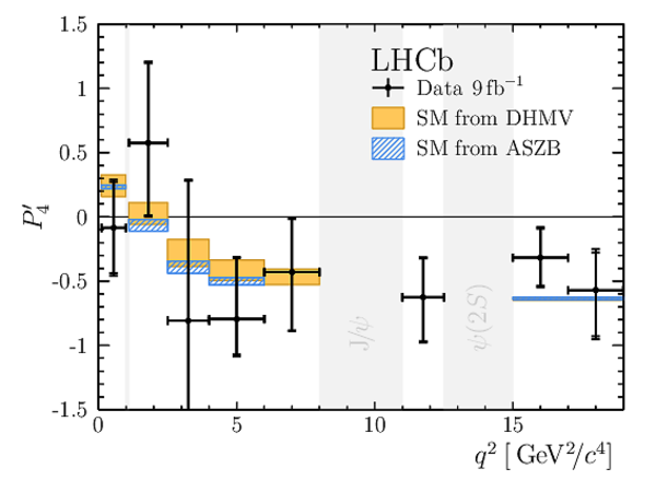
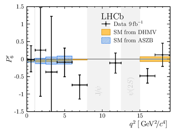
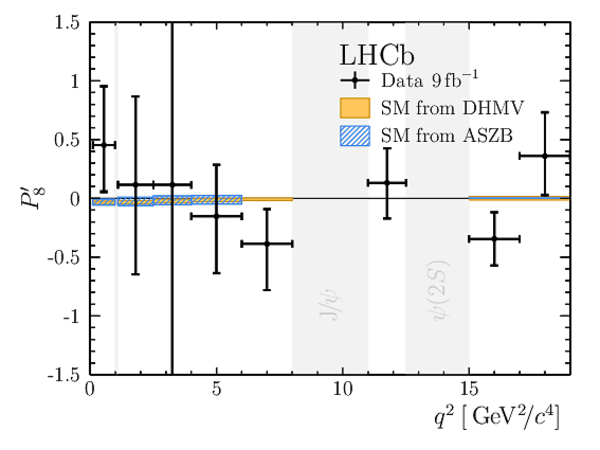
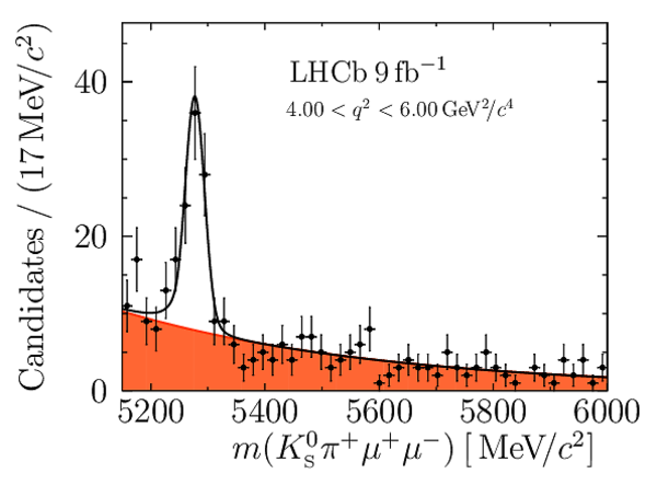
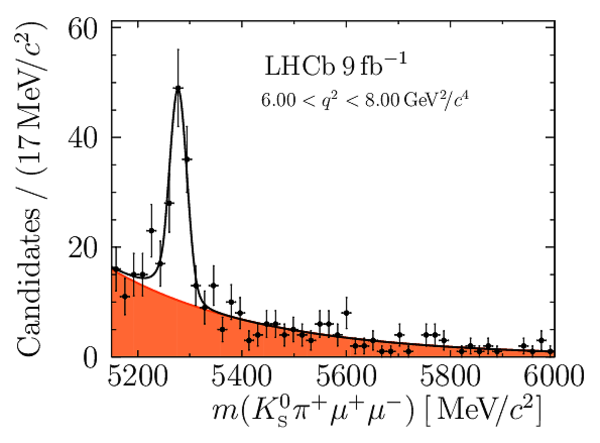
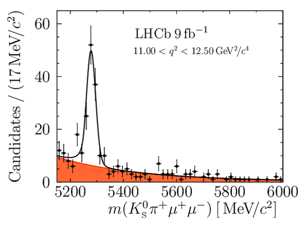
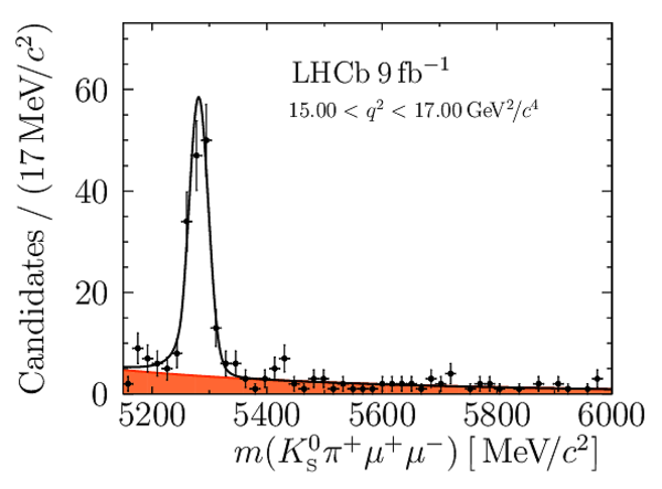
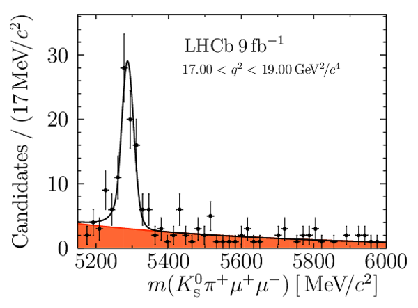
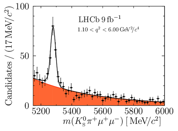
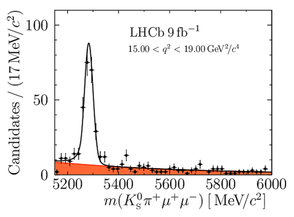
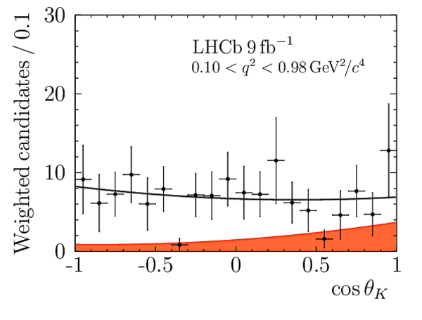
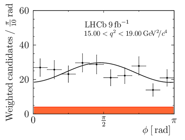
We present an angular analysis of the $B^{+}\rightarrow K^{\ast+}(\rightarrow K_{S}^{0}\pi^{+})\mu^{+}\mu^{-}$ decay using 9$ fb^{-1}$ of $pp$ collision data collected with the LHCb experiment. For the first time, the full set of CP-averaged angular observables is measured in intervals of the dimuon invariant mass squared. Local deviations from Standard Model predictions are observed, similar to those in previous LHCb analyses of the isospin-partner $B^{0}\rightarrow K^{\ast0}\mu^{+}\mu^{-}$ decay. The global tension is dependent on which effective couplings are considered and on the choice of theory nuisance parameters.
Figures and captions


![HiDef png [210 KiB]](Directory_LHCb-PAPER-2020-041/hidef_Fig1.png)
![HiDef png [204 KiB]](Directory_LHCb-PAPER-2020-041/hidef_Fig2a.png)
![HiDef png [234 KiB]](Directory_LHCb-PAPER-2020-041/hidef_Fig2b.png)
![HiDef png [217 KiB]](Directory_LHCb-PAPER-2020-041/hidef_Fig3a.png)
![HiDef png [150 KiB]](Directory_LHCb-PAPER-2020-041/hidef_Fig3b.png)
![HiDef png [153 KiB]](Directory_LHCb-PAPER-2020-041/hidef_Fig3c.png)
![HiDef png [170 KiB]](Directory_LHCb-PAPER-2020-041/hidef_Fig3d.png)
![HiDef png [170 KiB]](Directory_LHCb-PAPER-2020-041/hidef_Fig3e.png)
![HiDef png [162 KiB]](Directory_LHCb-PAPER-2020-041/hidef_Fig3f.png)
![HiDef png [147 KiB]](Directory_LHCb-PAPER-2020-041/hidef_Fig3g.png)
![HiDef png [136 KiB]](Directory_LHCb-PAPER-2020-041/hidef_Fig3h.png)
![HiDef png [218 KiB]](Directory_LHCb-PAPER-2020-041/hidef_Fig4a.png)
![HiDef png [209 KiB]](Directory_LHCb-PAPER-2020-041/hidef_Fig4b.png)
![HiDef png [204 KiB]](Directory_LHCb-PAPER-2020-041/hidef_Fig4c.png)
![HiDef png [166 KiB]](Directory_LHCb-PAPER-2020-041/hidef_Fig4d.png)
![HiDef png [190 KiB]](Directory_LHCb-PAPER-2020-041/hidef_Fig4e.png)
![HiDef png [234 KiB]](Directory_LHCb-PAPER-2020-041/hidef_Fig4f.png)
![HiDef png [214 KiB]](Directory_LHCb-PAPER-2020-041/hidef_Fig4g.png)
![HiDef png [182 KiB]](Directory_LHCb-PAPER-2020-041/hidef_Fig4h.png)
![HiDef png [213 KiB]](Directory_LHCb-PAPER-2020-041/hidef_Fig5a.png)
![HiDef png [226 KiB]](Directory_LHCb-PAPER-2020-041/hidef_Fig5b.png)
![HiDef png [231 KiB]](Directory_LHCb-PAPER-2020-041/hidef_Fig5c.png)
![HiDef png [231 KiB]](Directory_LHCb-PAPER-2020-041/hidef_Fig5d.png)
![HiDef png [227 KiB]](Directory_LHCb-PAPER-2020-041/hidef_Fig5e.png)
![HiDef png [220 KiB]](Directory_LHCb-PAPER-2020-041/hidef_Fig5f.png)
![HiDef png [215 KiB]](Directory_LHCb-PAPER-2020-041/hidef_Fig5g.png)
![HiDef png [226 KiB]](Directory_LHCb-PAPER-2020-041/hidef_Fig5h.png)
![HiDef png [227 KiB]](Directory_LHCb-PAPER-2020-041/hidef_Fig5i.png)
![HiDef png [217 KiB]](Directory_LHCb-PAPER-2020-041/hidef_Fig5j.png)
![HiDef png [169 KiB]](Directory_LHCb-PAPER-2020-041/hidef_Fig6a.png)
![HiDef png [182 KiB]](Directory_LHCb-PAPER-2020-041/hidef_Fig6b.png)
![HiDef png [186 KiB]](Directory_LHCb-PAPER-2020-041/hidef_Fig6c.png)
![HiDef png [179 KiB]](Directory_LHCb-PAPER-2020-041/hidef_Fig6d.png)
![HiDef png [178 KiB]](Directory_LHCb-PAPER-2020-041/hidef_Fig6e.png)
![HiDef png [172 KiB]](Directory_LHCb-PAPER-2020-041/hidef_Fig6f.png)
![HiDef png [150 KiB]](Directory_LHCb-PAPER-2020-041/hidef_Fig6g.png)
![HiDef png [169 KiB]](Directory_LHCb-PAPER-2020-041/hidef_Fig6h.png)
![HiDef png [177 KiB]](Directory_LHCb-PAPER-2020-041/hidef_Fig6i.png)
![HiDef png [162 KiB]](Directory_LHCb-PAPER-2020-041/hidef_Fig6j.png)
![HiDef png [174 KiB]](Directory_LHCb-PAPER-2020-041/hidef_Fig7a.png)
![HiDef png [167 KiB]](Directory_LHCb-PAPER-2020-041/hidef_Fig7b.png)
![HiDef png [188 KiB]](Directory_LHCb-PAPER-2020-041/hidef_Fig7c.png)
![HiDef png [168 KiB]](Directory_LHCb-PAPER-2020-041/hidef_Fig7d.png)
![HiDef png [175 KiB]](Directory_LHCb-PAPER-2020-041/hidef_Fig7e.png)
![HiDef png [167 KiB]](Directory_LHCb-PAPER-2020-041/hidef_Fig7f.png)
![HiDef png [157 KiB]](Directory_LHCb-PAPER-2020-041/hidef_Fig7g.png)
![HiDef png [158 KiB]](Directory_LHCb-PAPER-2020-041/hidef_Fig7h.png)
![HiDef png [174 KiB]](Directory_LHCb-PAPER-2020-041/hidef_Fig7i.png)
![HiDef png [161 KiB]](Directory_LHCb-PAPER-2020-041/hidef_Fig7j.png)
![HiDef png [127 KiB]](Directory_LHCb-PAPER-2020-041/hidef_Fig8a.png)
![HiDef png [133 KiB]](Directory_LHCb-PAPER-2020-041/hidef_Fig8b.png)
![HiDef png [134 KiB]](Directory_LHCb-PAPER-2020-041/hidef_Fig8c.png)
![HiDef png [127 KiB]](Directory_LHCb-PAPER-2020-041/hidef_Fig8d.png)
![HiDef png [127 KiB]](Directory_LHCb-PAPER-2020-041/hidef_Fig8e.png)
![HiDef png [126 KiB]](Directory_LHCb-PAPER-2020-041/hidef_Fig8f.png)
![HiDef png [124 KiB]](Directory_LHCb-PAPER-2020-041/hidef_Fig8g.png)
![HiDef png [128 KiB]](Directory_LHCb-PAPER-2020-041/hidef_Fig8h.png)
![HiDef png [122 KiB]](Directory_LHCb-PAPER-2020-041/hidef_Fig8i.png)
![HiDef png [130 KiB]](Directory_LHCb-PAPER-2020-041/hidef_Fig8j.png)
Tables and captions
|
Results for the $ C P$ -averaged observables $ F_{\rm L}$ , $ A_{\rm FB}$ and $S_{3} \text{--} S_{9}$. The first uncertainties are statistical and the second systematic. |
[Error creating the table] | |
|
Results for the optimised observables $ F_{\rm L}$ and $P_1\text{--}P_8^{\prime}$. The first uncertainties are statistical and the second systematic. |
[Error creating the table] | |
|
Correlation matrix for the $ C P$ -averaged observables $ F_{\rm L}$ , $ A_{\rm FB}$ and $S_{3} \text{--} S_{9}$ from the maximum-likelihood fit in the interval $0.10< q^2 <0.98\text{ Ge V} ^2 /c^4 $. |
Table_3.pdf [50 KiB] HiDef png [45 KiB] Thumbnail [21 KiB] tex code |

|
|
Correlation matrix for the $ C P$ -averaged observables $ F_{\rm L}$ , $ A_{\rm FB}$ and $S_{3} \text{--} S_{9}$ from the maximum-likelihood fit in the interval $1.1< q^2 <2.5\text{ Ge V} ^2 /c^4 $. |
Table_4.pdf [50 KiB] HiDef png [44 KiB] Thumbnail [20 KiB] tex code |

|
|
Correlation matrix for the $ C P$ -averaged observables $ F_{\rm L}$ , $ A_{\rm FB}$ and $S_{3} \text{--} S_{9}$ from the maximum-likelihood fit in the interval $2.5< q^2 <4.0\text{ Ge V} ^2 /c^4 $. |
Table_5.pdf [50 KiB] HiDef png [45 KiB] Thumbnail [21 KiB] tex code |

|
|
Correlation matrix for the $ C P$ -averaged observables $ F_{\rm L}$ , $ A_{\rm FB}$ and $S_{3} \text{--} S_{9}$ from the maximum-likelihood fit in the interval $4.0< q^2 <6.0\text{ Ge V} ^2 /c^4 $. |
Table_6.pdf [50 KiB] HiDef png [45 KiB] Thumbnail [21 KiB] tex code |

|
|
Correlation matrix for the $ C P$ -averaged observables $ F_{\rm L}$ , $ A_{\rm FB}$ and $S_{3} \text{--} S_{9}$ from the maximum-likelihood fit in the interval $6.0< q^2 <8.0\text{ Ge V} ^2 /c^4 $. |
Table_7.pdf [50 KiB] HiDef png [45 KiB] Thumbnail [21 KiB] tex code |

|
|
Correlation matrix for the $ C P$ -averaged observables $ F_{\rm L}$ , $ A_{\rm FB}$ and $S_{3} \text{--} S_{9}$ from the maximum-likelihood fit in the interval $11.0< q^2 <12.5\text{ Ge V} ^2 /c^4 $. |
Table_8.pdf [50 KiB] HiDef png [45 KiB] Thumbnail [21 KiB] tex code |

|
|
Correlation matrix for the $ C P$ -averaged observables $ F_{\rm L}$ , $ A_{\rm FB}$ and $S_{3} \text{--} S_{9}$ from the maximum-likelihood fit in the interval $15.0< q^2 <17.0\text{ Ge V} ^2 /c^4 $. |
Table_9.pdf [50 KiB] HiDef png [45 KiB] Thumbnail [21 KiB] tex code |

|
|
Correlation matrix for the $ C P$ -averaged observables $ F_{\rm L}$ , $ A_{\rm FB}$ and $S_{3} \text{--} S_{9}$ from the maximum-likelihood fit in the interval $17.0< q^2 <19.0\text{ Ge V} ^2 /c^4 $. |
Table_10.pdf [50 KiB] HiDef png [44 KiB] Thumbnail [21 KiB] tex code |

|
|
Correlation matrix for the $ C P$ -averaged observables $ F_{\rm L}$ , $ A_{\rm FB}$ and $S_{3} \text{--} S_{9}$ from the maximum-likelihood fit in the interval $1.1< q^2 <6.0\text{ Ge V} ^2 /c^4 $. |
Table_11.pdf [50 KiB] HiDef png [45 KiB] Thumbnail [21 KiB] tex code |

|
|
Correlation matrix for the $ C P$ -averaged observables $ F_{\rm L}$ , $ A_{\rm FB}$ and $S_{3} \text{--} S_{9}$ from the maximum-likelihood fit in the interval $15.0< q^2 <19.0\text{ Ge V} ^2 /c^4 $. |
Table_12.pdf [50 KiB] HiDef png [45 KiB] Thumbnail [21 KiB] tex code |

|
|
Correlation matrix for the $ C P$ -averaged observables $ F_{\rm L}$ and $P_{i}^{(\prime)}$ from the maximum-likelihood fit in the interval $0.10< q^2 <0.98\text{ Ge V} ^2 /c^4 $. |
Table_13.pdf [57 KiB] HiDef png [45 KiB] Thumbnail [22 KiB] tex code |

|
|
Correlation matrix for the $ C P$ -averaged observables $ F_{\rm L}$ and $P_{i}^{(\prime)}$ from the maximum-likelihood fit in the interval $1.1< q^2 <2.5\text{ Ge V} ^2 /c^4 $. |
Table_14.pdf [57 KiB] HiDef png [45 KiB] Thumbnail [22 KiB] tex code |

|
|
Correlation matrix for the $ C P$ -averaged observables $ F_{\rm L}$ and $P_{i}^{(\prime)}$ from the maximum-likelihood fit in the interval $2.5< q^2 <4.0\text{ Ge V} ^2 /c^4 $. |
Table_15.pdf [56 KiB] HiDef png [46 KiB] Thumbnail [22 KiB] tex code |

|
|
Correlation matrix for the $ C P$ -averaged observables $ F_{\rm L}$ and $P_{i}^{(\prime)}$ from the maximum-likelihood fit in the interval $4.0< q^2 <6.0\text{ Ge V} ^2 /c^4 $. |
Table_16.pdf [57 KiB] HiDef png [45 KiB] Thumbnail [22 KiB] tex code |

|
|
Correlation matrix for the $ C P$ -averaged observables $ F_{\rm L}$ and $P_{i}^{(\prime)}$ from the maximum-likelihood fit in the interval $6.0< q^2 <8.0\text{ Ge V} ^2 /c^4 $. |
Table_17.pdf [56 KiB] HiDef png [45 KiB] Thumbnail [21 KiB] tex code |

|
|
Correlation matrix for the $ C P$ -averaged observables $ F_{\rm L}$ and $P_{i}^{(\prime)}$ from the maximum-likelihood fit in the interval $11.0< q^2 <12.5\text{ Ge V} ^2 /c^4 $. |
Table_18.pdf [56 KiB] HiDef png [45 KiB] Thumbnail [22 KiB] tex code |

|
|
Correlation matrix for the $ C P$ -averaged observables $ F_{\rm L}$ and $P_{i}^{(\prime)}$ from the maximum-likelihood fit in the interval $15.0< q^2 <17.0\text{ Ge V} ^2 /c^4 $. |
Table_19.pdf [56 KiB] HiDef png [45 KiB] Thumbnail [22 KiB] tex code |

|
|
Correlation matrix for the $ C P$ -averaged observables $ F_{\rm L}$ and $P_{i}^{(\prime)}$ from the maximum-likelihood fit in the interval $17.0< q^2 <19.0\text{ Ge V} ^2 /c^4 $. |
Table_20.pdf [57 KiB] HiDef png [46 KiB] Thumbnail [22 KiB] tex code |

|
|
Correlation matrix for the $ C P$ -averaged observables $ F_{\rm L}$ and $P_{i}^{(\prime)}$ from the maximum-likelihood fit in the interval $1.1< q^2 <6.0\text{ Ge V} ^2 /c^4 $. |
Table_21.pdf [57 KiB] HiDef png [43 KiB] Thumbnail [21 KiB] tex code |

|
|
Correlation matrix for the $ C P$ -averaged observables $ F_{\rm L}$ and $P_{i}^{(\prime)}$ from the maximum-likelihood fit in the interval $15.0< q^2 <19.0\text{ Ge V} ^2 /c^4 $. |
Table_22.pdf [57 KiB] HiDef png [45 KiB] Thumbnail [21 KiB] tex code |

|
|
Maximum values for each source of systematic uncertainty. |
Table_23.pdf [61 KiB] HiDef png [94 KiB] Thumbnail [39 KiB] tex code |

|
|
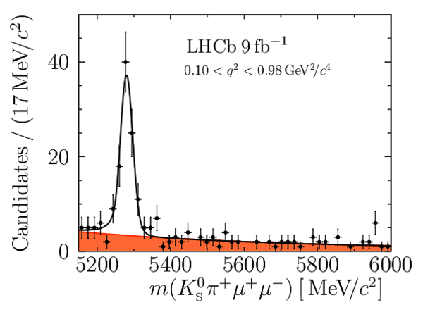
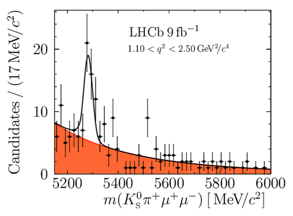
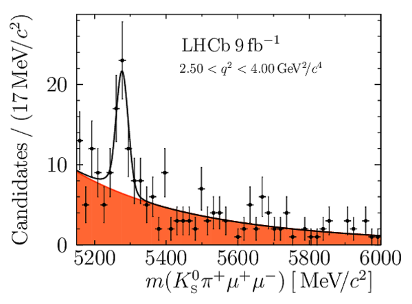
Yields of signal candidates in the ten $ q^2$ intervals. They are obtained from extended maximum-likelihood fits to the $m( K ^0_{\mathrm{S}} \pi ^+ \mu ^+\mu ^- )$ distribution. The total number corresponds to the sum of the eight nominal $ q^2$ intervals. |
Table_24.pdf [53 KiB] HiDef png [163 KiB] Thumbnail [78 KiB] tex code |

|
![HiDef png [45 KiB]](Directory_LHCb-PAPER-2020-041/hidef_Table_3.png)
![HiDef png [44 KiB]](Directory_LHCb-PAPER-2020-041/hidef_Table_4.png)
![HiDef png [45 KiB]](Directory_LHCb-PAPER-2020-041/hidef_Table_5.png)
![HiDef png [45 KiB]](Directory_LHCb-PAPER-2020-041/hidef_Table_6.png)
![HiDef png [45 KiB]](Directory_LHCb-PAPER-2020-041/hidef_Table_7.png)
![HiDef png [45 KiB]](Directory_LHCb-PAPER-2020-041/hidef_Table_8.png)
![HiDef png [45 KiB]](Directory_LHCb-PAPER-2020-041/hidef_Table_9.png)
![HiDef png [44 KiB]](Directory_LHCb-PAPER-2020-041/hidef_Table_10.png)
![HiDef png [45 KiB]](Directory_LHCb-PAPER-2020-041/hidef_Table_11.png)
![HiDef png [45 KiB]](Directory_LHCb-PAPER-2020-041/hidef_Table_12.png)
![HiDef png [45 KiB]](Directory_LHCb-PAPER-2020-041/hidef_Table_13.png)
![HiDef png [45 KiB]](Directory_LHCb-PAPER-2020-041/hidef_Table_14.png)
![HiDef png [46 KiB]](Directory_LHCb-PAPER-2020-041/hidef_Table_15.png)
![HiDef png [45 KiB]](Directory_LHCb-PAPER-2020-041/hidef_Table_16.png)
![HiDef png [45 KiB]](Directory_LHCb-PAPER-2020-041/hidef_Table_17.png)
![HiDef png [45 KiB]](Directory_LHCb-PAPER-2020-041/hidef_Table_18.png)
![HiDef png [45 KiB]](Directory_LHCb-PAPER-2020-041/hidef_Table_19.png)
![HiDef png [46 KiB]](Directory_LHCb-PAPER-2020-041/hidef_Table_20.png)
![HiDef png [43 KiB]](Directory_LHCb-PAPER-2020-041/hidef_Table_21.png)
![HiDef png [45 KiB]](Directory_LHCb-PAPER-2020-041/hidef_Table_22.png)
![HiDef png [94 KiB]](Directory_LHCb-PAPER-2020-041/hidef_Table_23.png)
![HiDef png [163 KiB]](Directory_LHCb-PAPER-2020-041/hidef_Table_24.png)
Supplementary Material [file]
| Supplementary material full pdf |
Supple[..].pdf [208 KiB] |
|
|
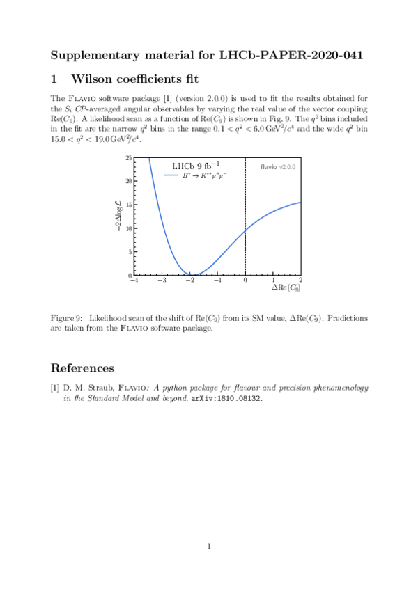
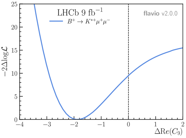
This ZIP file contains supplementary material for the publication LHCb-PAPER-2020-041. The files are: Supplementary.pdf : An overview of the extra figures Supplementary.tex : the LaTeX code of the supplementary material Fig9.pdf, Fig9.png, Fig9.eps : Figure 9 in various graphic formats Fig9.py, Fig9.csv : Figure 9 as python macro plus data values |
Fig9.pdf [146 KiB] HiDef png [160 KiB] Thumbnail [107 KiB] *C file |
|
![HiDef png [160 KiB]](Directory_LHCb-PAPER-2020-041/supplementary/hidef_Fig9.png)
Created on 20 April 2024.