Angular analysis of $ {B}^0\to {D}^{\ast -}{D}_s^{\ast +} $ with $ {D}_s^{\ast +}\to {D}_s^{+}\gamma $ decays
[to restricted-access page]Information
LHCb-PAPER-2021-006
CERN-EP-2021-056
arXiv:2105.02596 [PDF]
(Submitted on 06 May 2021)
JHEP 06 (2021) 177
Inspire 1862311
Tools
Abstract
The first full angular analysis of the $B^0 \to D^{*-} D_s^{*+}$ decay is performed using 6 fb$^{-1}$ of $pp$ collision data collected with the LHCb experiment at a centre-of-mass energy of 13 TeV. The $D_s^{*+} \to D_s^+ \gamma$ and $D^{*-} \to \bar{D}^0 \pi^-$ vector meson decays are used with the subsequent $D_s^+ \to K^+ K^- \pi^+$ and $\bar{D}^0 \to K^+ \pi^-$ decays. All helicity amplitudes and phases are measured, and the longitudinal polarisation fraction is determined to be $f_{\rm L} = 0.578 \pm 0.010 \pm 0.011$ with world-best precision, where the first uncertainty is statistical and the second is systematic. The pattern of helicity amplitude magnitudes is found to align with expectations from quark-helicity conservation in $B$ decays. The ratio of branching fractions $[\mathcal{B}(B^0 \to D^{*-} D_s^{*+}) \times \mathcal{B}(D_s^{*+} \to D_s^+ \gamma)]/\mathcal{B}(B^0 \to D^{*-} D_s^+)$ is measured to be $2.045 \pm 0.022 \pm 0.071$ with world-best precision. In addition, the first observation of the Cabibbo-suppressed $B_s^0 \to D^{*-} D_s^+$ decay is made with a significance of seven standard deviations. The branching fraction ratio $\mathcal{B}(B_s^0 \to D^{*-} D_s^+)/\mathcal{B}(B^0 \to D^{*-} D_s^+)$ is measured to be $0.049 \pm 0.006 \pm 0.003 \pm 0.002$, where the third uncertainty is due to limited knowledge of the ratio of fragmentation fractions.
Figures and captions
|
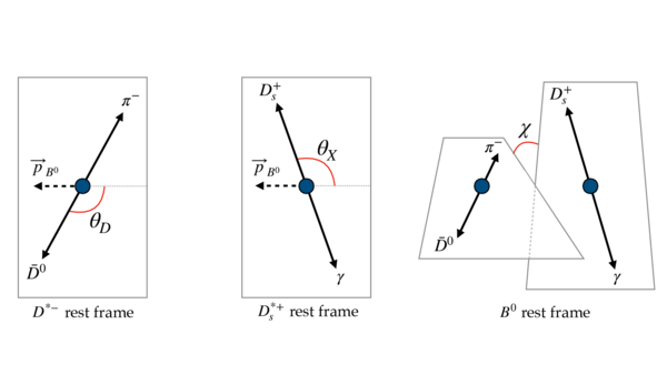
Illustration of the $ B^0 \rightarrow D^{*-} D_s^{*+}$ decay angles. |
Fig1.pdf [81 KiB] Thumbnail [73 KiB] *.C file |
|
|
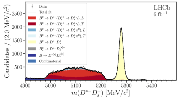
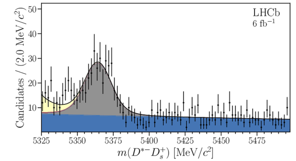
(Top) Distribution of $m(D^{*-}D_s^+)$ for selected candidates in data, with the fit overlaid. Where indicated, $L$ ($T$) represents longitudinally (transverse) polarised decays. (Bottom) Restricted to region for candidates with $m(D^{*-}D_s^+) > 5325$ $\text{ Me V /}c^2$ , where the Cabibbo-suppressed $B_s^0 \rightarrow D^{*-} D_s^+$ contribution is visible. |
Fig2a.pdf [276 KiB] HiDef png [222 KiB] Thumbnail [164 KiB] *.C file |
|
|
Fig2b.pdf [207 KiB] HiDef png [197 KiB] Thumbnail [142 KiB] *.C file |
|
|
|
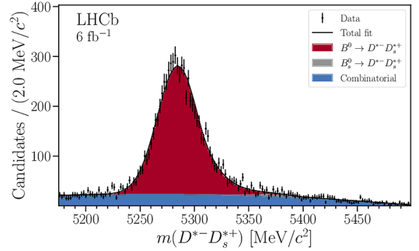
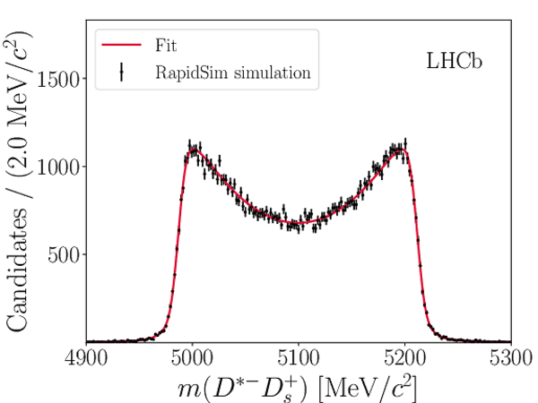
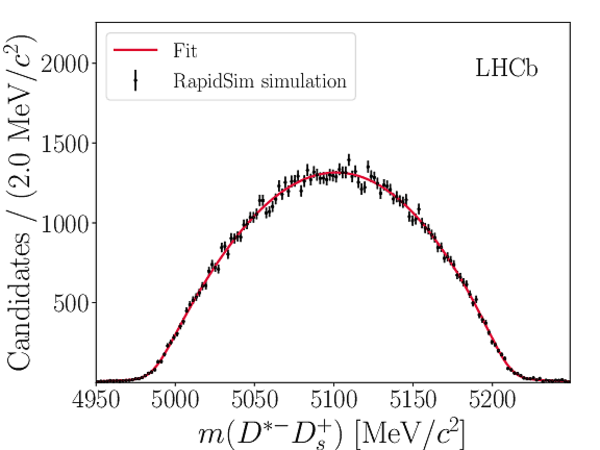
Distribution of $m(D^{*-}D_s^{*+})$ for selected candidates in data, with the fit overlaid. |
Fig3.pdf [209 KiB] HiDef png [203 KiB] Thumbnail [145 KiB] *.C file |
|
|
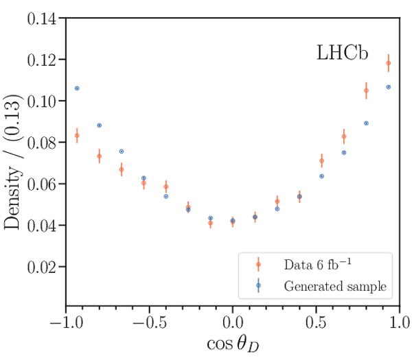
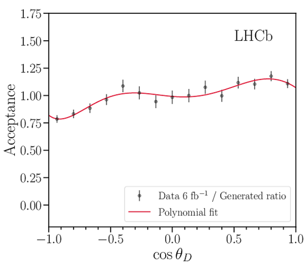
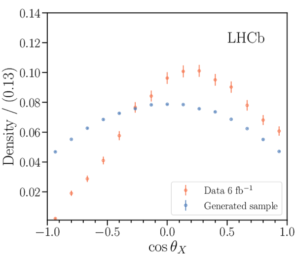
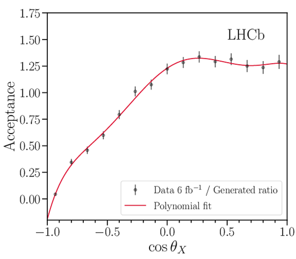
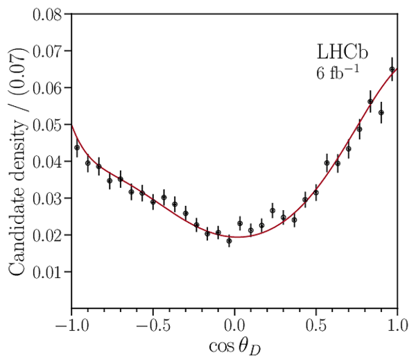
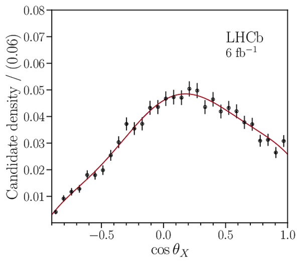
(Left) Comparison of signal-weighted data and generated (top) $\cos\theta_D$ and (bottom) $\cos\theta_X$ distributions, where the differences observed are due to the experimental acceptance and resolution. (Right) Data to generated sample ratios, with the polynomial fits overlaid. |
Fig4a.pdf [128 KiB] HiDef png [131 KiB] Thumbnail [108 KiB] *.C file |
|
|
Fig4b.pdf [128 KiB] HiDef png [147 KiB] Thumbnail [121 KiB] *.C file |
|
|
|
Fig4c.pdf [128 KiB] HiDef png [133 KiB] Thumbnail [109 KiB] *.C file |
|
|
|
Fig4d.pdf [128 KiB] HiDef png [160 KiB] Thumbnail [127 KiB] *.C file |
|
|
|
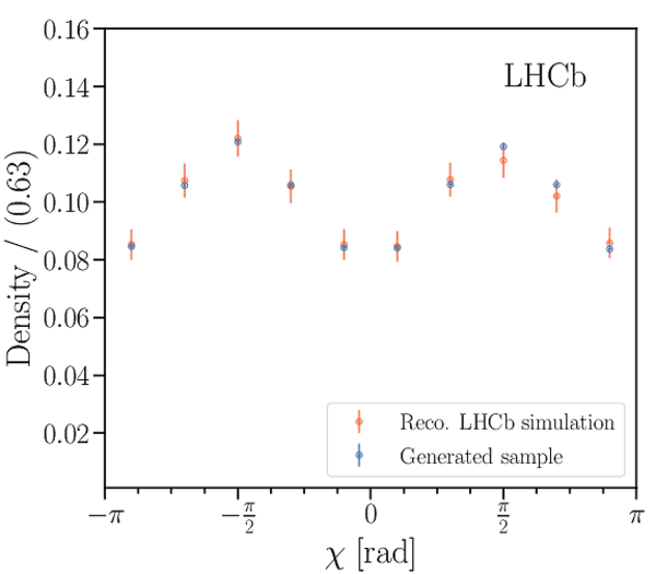
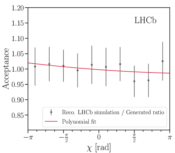
Comparison of reconstructed $\chi$ distribution in a fully-simulated $ B^0 \rightarrow D^{*-} D_s^{*+}$ sample and the generated $\chi$ distribution in a RapidSim sample produced with the same helicity amplitude model (left). The ratio is fitted with a second-order polynomial to determine the acceptance function for use in the data fit (right). |
Fig5a.pdf [98 KiB] HiDef png [127 KiB] Thumbnail [106 KiB] *.C file |
|
|
Fig5b.pdf [97 KiB] HiDef png [147 KiB] Thumbnail [119 KiB] *.C file |
|
|
|
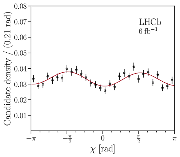
Decay-angle distributions of signal-weighted $ B^0 \rightarrow D^{*-} D_s^{*+}$ candidates in data, with the one-dimensional angular fit projections overlaid. |
Fig6a.pdf [98 KiB] HiDef png [158 KiB] Thumbnail [133 KiB] *.C file |
|
|
Fig6b.pdf [98 KiB] HiDef png [157 KiB] Thumbnail [133 KiB] *.C file |
|
|
|
Fig6c.pdf [98 KiB] HiDef png [151 KiB] Thumbnail [130 KiB] *.C file |
|
|
|
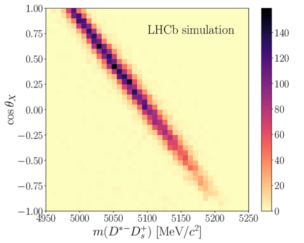
Relationship between $m(D^{*-}D_s^+)$ and $\cos\theta_X$ in a sample of fully reconstructed $B^0 \rightarrow D^{*-} (D_s^{*+} \rightarrow D_s^+ \gamma)$ simulated decays. The colour scale indicates the number of candidates in each bin. |
Fig7.pdf [119 KiB] HiDef png [275 KiB] Thumbnail [184 KiB] *.C file |
|
|
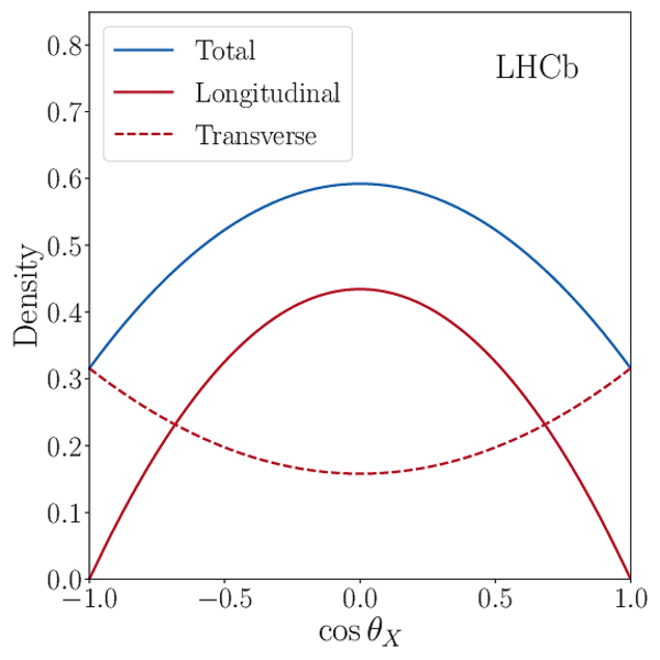
Transverse and longitudinal contributions to the one-dimensional decay rate shown as a function of $\cos\theta_X$. |
Fig8.pdf [98 KiB] HiDef png [247 KiB] Thumbnail [154 KiB] *.C file |
|
|
Invariant-mass distributions of (left) pure transverse and (right) longitudinal $B^0 \rightarrow D^{*-} (D_s^{*+} \rightarrow D_s^+ \gamma)$ simulated decays. Fits to the distributions are overlaid, from which shape parameters for use in the $m(D^{*-}D_s^+)$ data fit are derived. |
Fig9a.pdf [102 KiB] HiDef png [210 KiB] Thumbnail [152 KiB] *.C file |
|
|
Fig9b.pdf [101 KiB] HiDef png [194 KiB] Thumbnail [151 KiB] *.C file |
|
|
|
Animated gif made out of all figures. |
PAPER-2021-006.gif Thumbnail |

|
![HiDef png [222 KiB]](Directory_LHCb-PAPER-2021-006/hidef_Fig2a.png)
![HiDef png [197 KiB]](Directory_LHCb-PAPER-2021-006/hidef_Fig2b.png)
![HiDef png [203 KiB]](Directory_LHCb-PAPER-2021-006/hidef_Fig3.png)
![HiDef png [131 KiB]](Directory_LHCb-PAPER-2021-006/hidef_Fig4a.png)
![HiDef png [147 KiB]](Directory_LHCb-PAPER-2021-006/hidef_Fig4b.png)
![HiDef png [133 KiB]](Directory_LHCb-PAPER-2021-006/hidef_Fig4c.png)
![HiDef png [160 KiB]](Directory_LHCb-PAPER-2021-006/hidef_Fig4d.png)
![HiDef png [127 KiB]](Directory_LHCb-PAPER-2021-006/hidef_Fig5a.png)
![HiDef png [147 KiB]](Directory_LHCb-PAPER-2021-006/hidef_Fig5b.png)
![HiDef png [158 KiB]](Directory_LHCb-PAPER-2021-006/hidef_Fig6a.png)
![HiDef png [157 KiB]](Directory_LHCb-PAPER-2021-006/hidef_Fig6b.png)
![HiDef png [151 KiB]](Directory_LHCb-PAPER-2021-006/hidef_Fig6c.png)
![HiDef png [275 KiB]](Directory_LHCb-PAPER-2021-006/hidef_Fig7.png)
![HiDef png [247 KiB]](Directory_LHCb-PAPER-2021-006/hidef_Fig8.png)
![HiDef png [210 KiB]](Directory_LHCb-PAPER-2021-006/hidef_Fig9a.png)
![HiDef png [194 KiB]](Directory_LHCb-PAPER-2021-006/hidef_Fig9b.png)
Tables and captions
|
Systematic uncertainties on the branching fraction ratios and $f_L$ as measured in the $m(D^{*-} D_s^+)$ fit. |
Table_1.pdf [63 KiB] HiDef png [68 KiB] Thumbnail [29 KiB] tex code |

|
|
Systematic uncertainties on the helicity parameters measured in the unbinned angular fit. |
Table_2.pdf [72 KiB] HiDef png [64 KiB] Thumbnail [27 KiB] tex code |

|
![HiDef png [68 KiB]](Directory_LHCb-PAPER-2021-006/hidef_Table_1.png)
![HiDef png [64 KiB]](Directory_LHCb-PAPER-2021-006/hidef_Table_2.png)
Created on 18 April 2024.