Information
LHCb-PAPER-2021-022
CERN-EP-2021-138
arXiv:2107.13428 [PDF]
(Submitted on 28 Jul 2021)
JHEP 11 (2021) 043
Inspire 1894428
Tools
Abstract
An angular analysis of the rare decay $B^0_s\rightarrow\phi\mu^+\mu^-$ is presented, using proton-proton collision data collected by the LHCb experiment at centre-of-mass energies of $7$, $8$ and $13 \rm{TeV}$, corresponding to an integrated luminosity of $8.4 \rm{fb}^{-1}$. The observables describing the angular distributions of the decay $B^0_s\rightarrow\phi\mu^+\mu^-$ are determined in regions of $q^2$, the square of the dimuon invariant mass. The results are consistent with Standard Model predictions.
Figures and captions
|
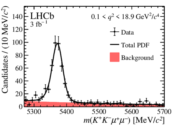
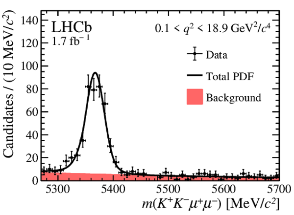
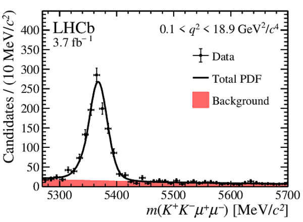
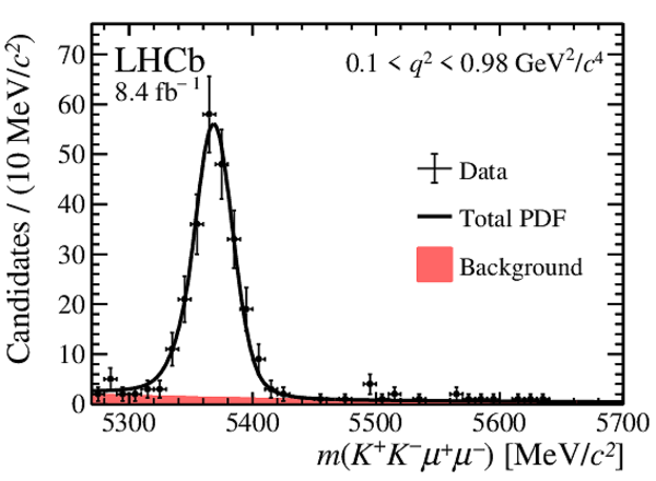
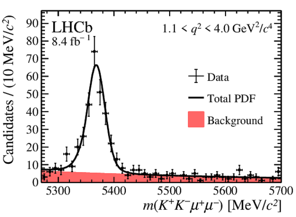
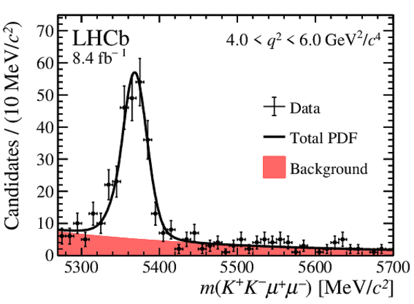
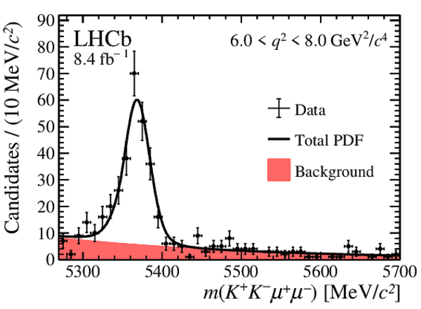
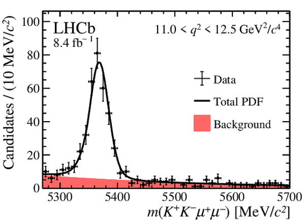
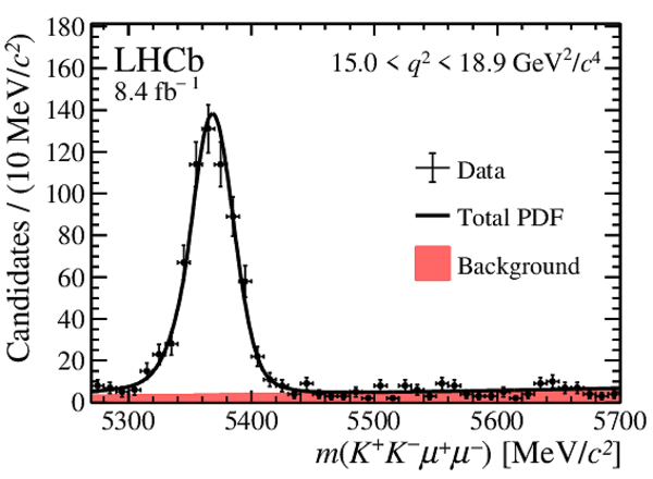
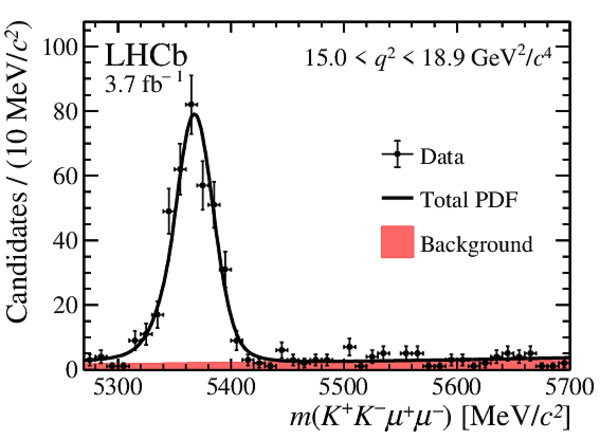
The $m( K ^+ K ^- \mu ^+\mu ^- )$ distribution for $ B ^0_ s \rightarrow \phi\mu ^+ \mu ^- $ candidates integrated over the $0.1 < q^2 <0.98\text{ Ge V} ^2 /c^4 $, $1.1 < q^2 <8\text{ Ge V} ^2 /c^4 $, $11.0 < q^2 < 12.5\text{ Ge V} ^2 /c^4 $ and $15.0 < q^2 <18.9\text{ Ge V} ^2 /c^4 $ regions for the data-taking periods 2011-2012 (top left), 2016 (top right), and 2017--2018 (bottom). The data are overlaid with the PDF used to describe the $m( K ^+ K ^- \mu ^+\mu ^- )$ spectrum, fitted separately for each data set. |
Fig1a.pdf [18 KiB] HiDef png [226 KiB] Thumbnail [217 KiB] *.C file |
|
|
Fig1b.pdf [18 KiB] HiDef png [222 KiB] Thumbnail [215 KiB] *.C file |
|
|
|
Fig1c.pdf [18 KiB] HiDef png [223 KiB] Thumbnail [220 KiB] *.C file |
|
|
|
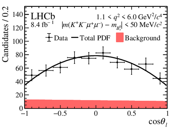
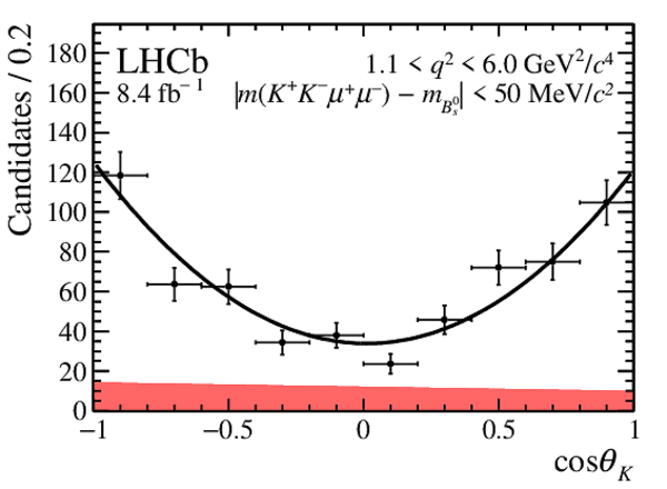
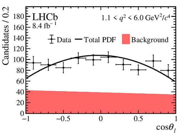
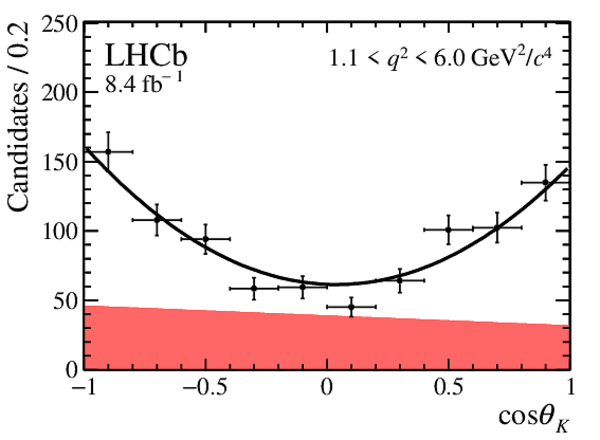
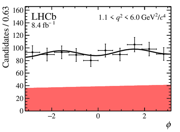
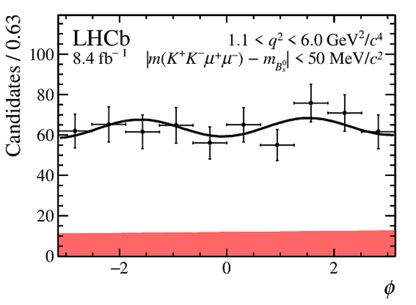
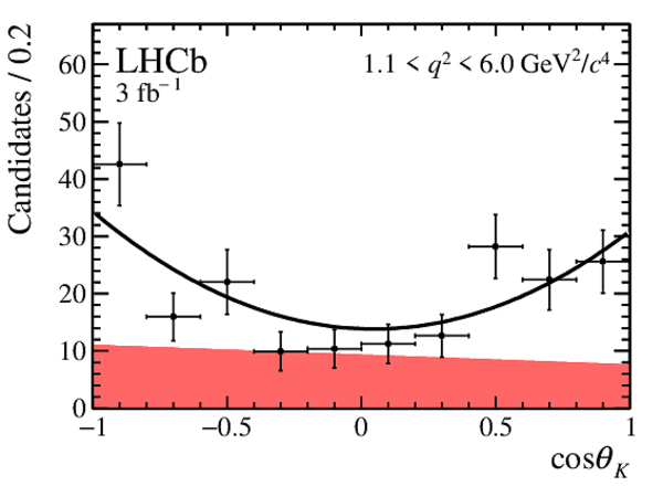
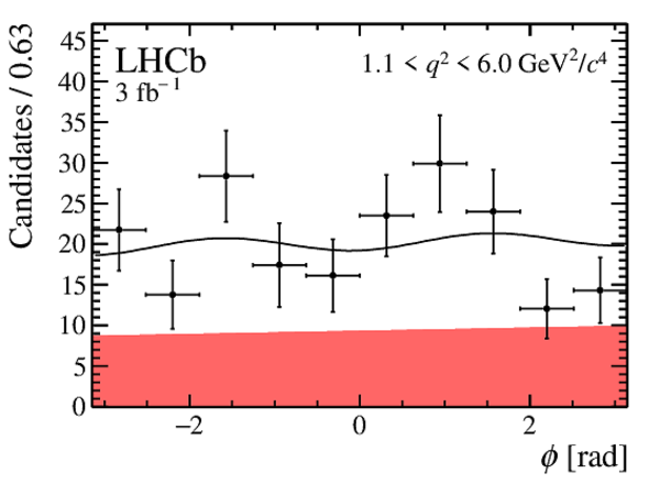
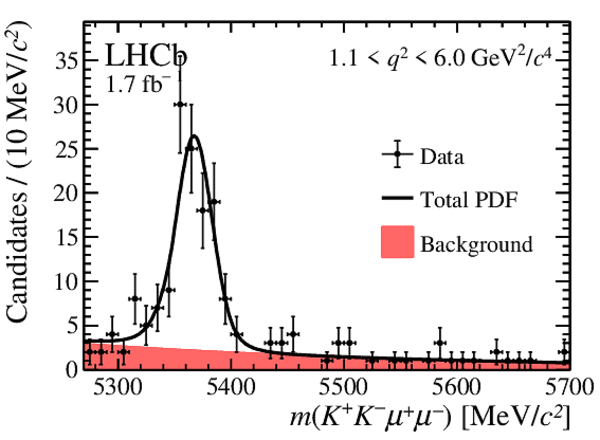
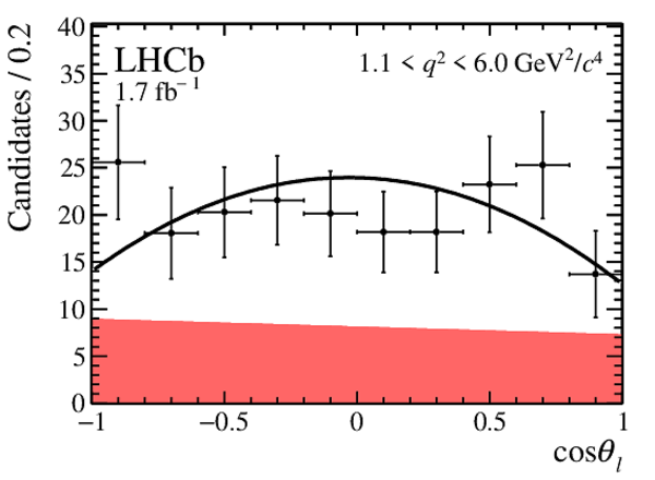
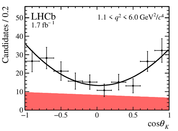
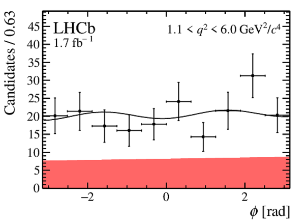
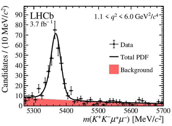
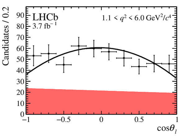
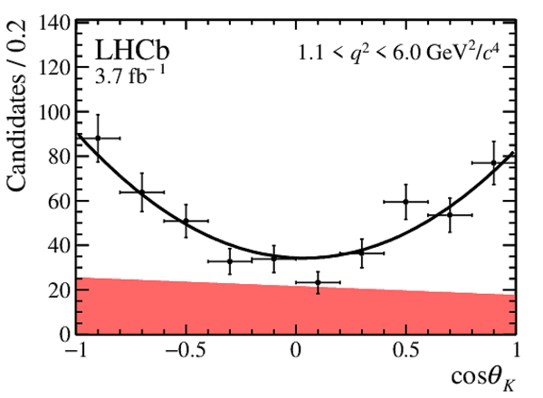
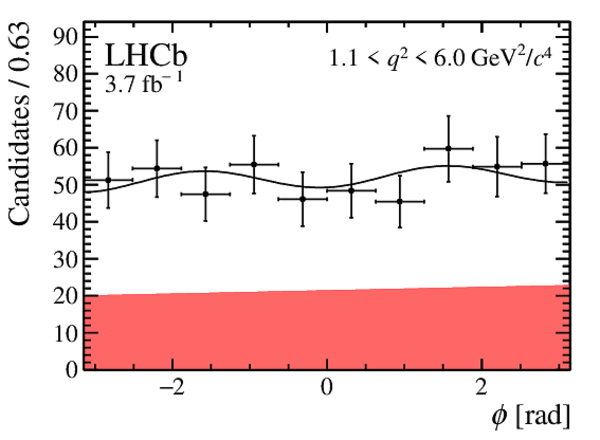
Angular projections in the region $1.1 < q^2 <6.0\text{ Ge V} ^2 /c^4 $ for the combined 2011--2012, 2016 and 2017--2018 data sets. The data are overlaid with the projection of the combined PDF. The red shaded area indicates the background component and the solid black line the total PDF. The angular projections are given for candidates in (left) the entire mass region used to determine the observables in this paper and (right) the signal mass window $\pm50\text{ Me V /}c^2 $ around the known $ B ^0_ s $ mass. |
Fig2a.pdf [13 KiB] HiDef png [168 KiB] Thumbnail [174 KiB] *.C file |

|
|
Fig2d.pdf [14 KiB] HiDef png [178 KiB] Thumbnail [183 KiB] *.C file |
|
|
|
Fig2b.pdf [12 KiB] HiDef png [137 KiB] Thumbnail [141 KiB] *.C file |

|
|
|
Fig2e.pdf [13 KiB] HiDef png [169 KiB] Thumbnail [178 KiB] *.C file |
|
|
|
Fig2c.pdf [11 KiB] HiDef png [132 KiB] Thumbnail [133 KiB] *.C file |

|
|
|
Fig2f.pdf [12 KiB] HiDef png [141 KiB] Thumbnail [141 KiB] *.C file |

|
|
|
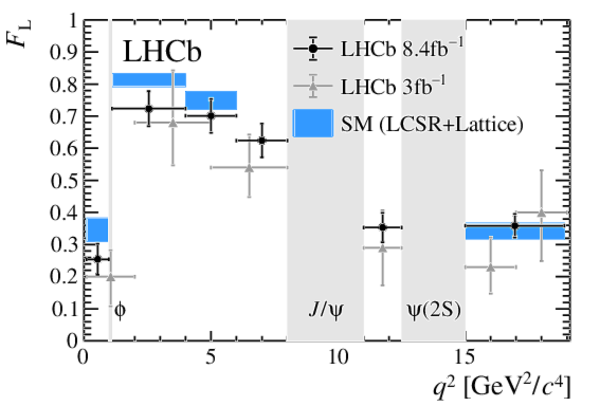
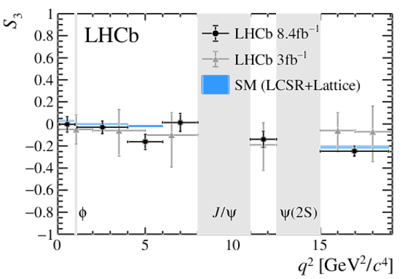
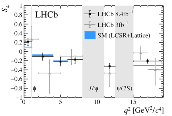
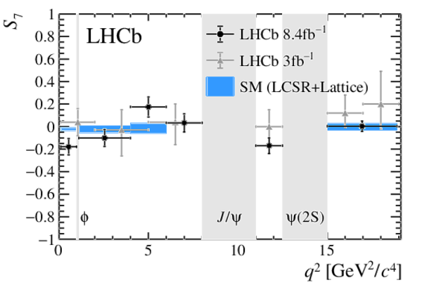
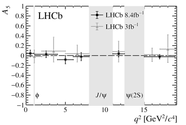
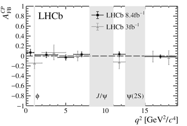
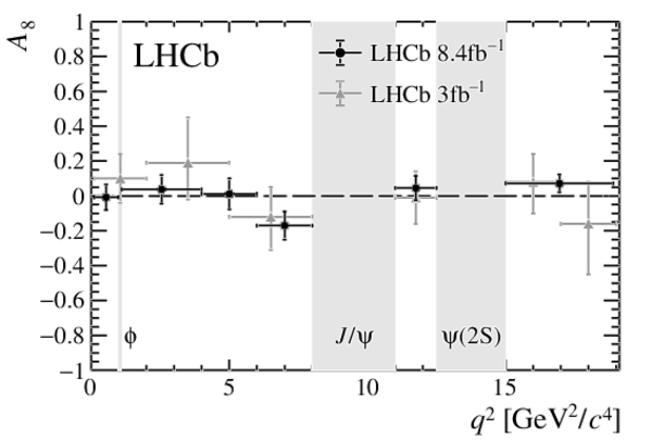
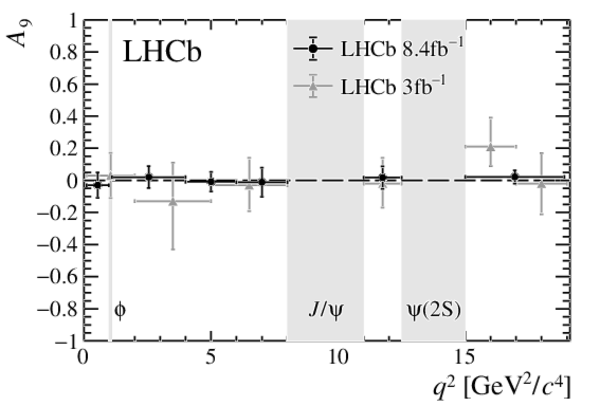
$ C P$ -averaged angular observables $ F_{\mathrm{L}}$ and $S_{3,4,7}$ and $ C P$ -asymmetries $ A_{\mathrm{FB}}^{ C P }$ and $A_{5,8,9}$ shown by black crosses, overlaid with the SM prediction [23,24,25,26] as blue boxes, where available. The grey crosses indicate the results from Ref. [4]. The grey bands indicate the regions of the charmonium resonances and the $ B ^0_ s \rightarrow \phi\phi$ region. |
Fig3a.pdf [16 KiB] HiDef png [220 KiB] Thumbnail [192 KiB] *.C file |
|
|
Fig3b.pdf [16 KiB] HiDef png [212 KiB] Thumbnail [185 KiB] *.C file |
|
|
|
Fig3c.pdf [16 KiB] HiDef png [212 KiB] Thumbnail [185 KiB] *.C file |
|
|
|
Fig3d.pdf [16 KiB] HiDef png [214 KiB] Thumbnail [186 KiB] *.C file |
|
|
|
Fig3e.pdf [15 KiB] HiDef png [150 KiB] Thumbnail [93 KiB] *.C file |
|
|
|
Fig3f.pdf [15 KiB] HiDef png [152 KiB] Thumbnail [93 KiB] *.C file |
|
|
|
Fig3g.pdf [15 KiB] HiDef png [150 KiB] Thumbnail [93 KiB] *.C file |
|
|
|
Fig3h.pdf [15 KiB] HiDef png [149 KiB] Thumbnail [91 KiB] *.C file |
|
|
|
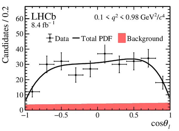
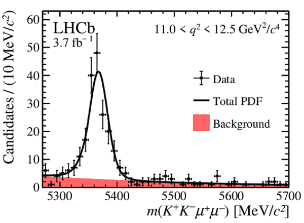
Mass distributions of $ B ^0_ s \rightarrow \phi\mu ^+ \mu ^- $ candidates in the different $ q^2$ regions for the combined 2011--2012, 2016 and 2017--2018 data sets. The data are overlaid with the projection of the combined PDF. The red shaded area indicates the background component and the solid black line the total PDF. |
Fig4a.pdf [17 KiB] HiDef png [210 KiB] Thumbnail [208 KiB] *.C file |
|
|
Fig4b.pdf [18 KiB] HiDef png [238 KiB] Thumbnail [233 KiB] *.C file |
|
|
|
Fig4c.pdf [19 KiB] HiDef png [241 KiB] Thumbnail [232 KiB] *.C file |
|
|
|
Fig4d.pdf [19 KiB] HiDef png [239 KiB] Thumbnail [232 KiB] *.C file |
|
|
|
Fig4e.pdf [18 KiB] HiDef png [223 KiB] Thumbnail [210 KiB] *.C file |
|
|
|
Fig4f.pdf [19 KiB] HiDef png [239 KiB] Thumbnail [227 KiB] *.C file |

|
|
|
Fig4g.pdf [18 KiB] HiDef png [235 KiB] Thumbnail [225 KiB] *.C file |
|
|
|
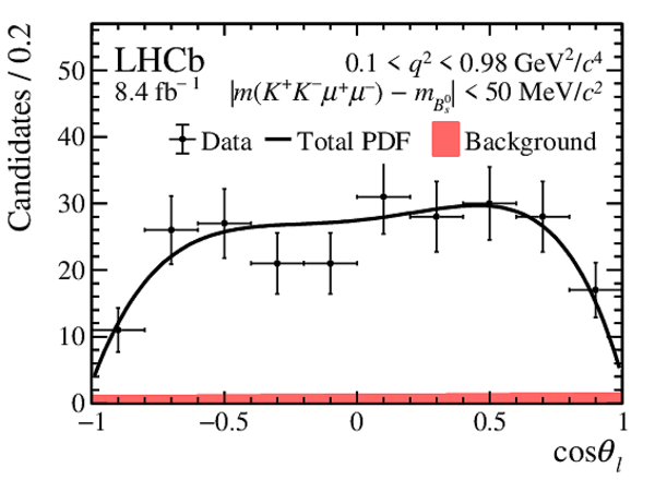
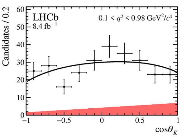
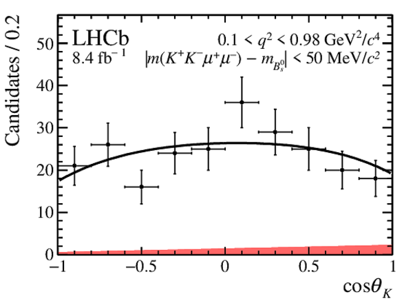
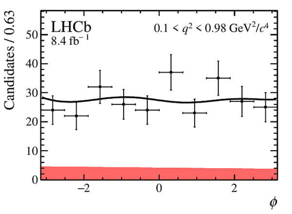
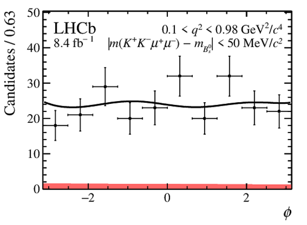
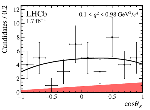
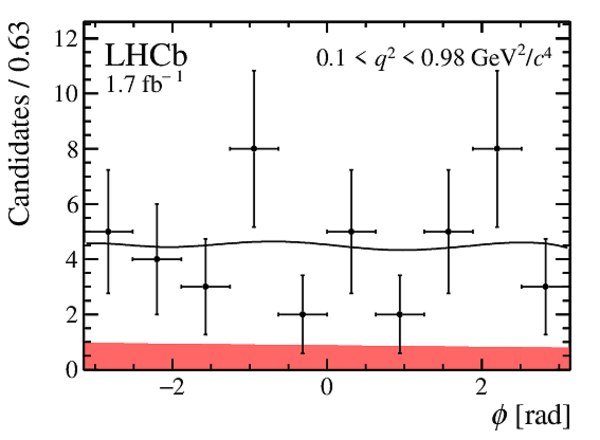
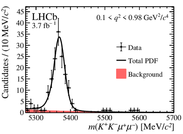
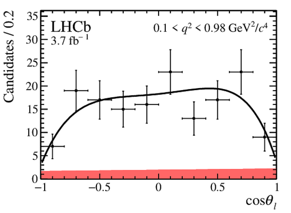
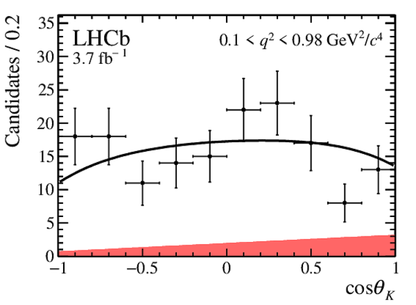
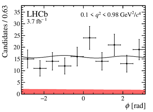
Projections in the region $0.1 < q^2 <0.98\text{ Ge V} ^2 /c^4 $ for the angular distributions of the combined 2011--2012, 2016 and 2017--2018 data sets. The data are overlaid with the projection of the combined PDF. The red shaded area indicates the background component and the solid black line the total PDF. The angular projections are given for candidates in (left) the entire mass region used to determine the observables in this paper and (right) the signal mass window $\pm50\text{ Me V /}c^2 $ around the known $ B ^0_ s $ mass. |
Fig5a.pdf [13 KiB] HiDef png [158 KiB] Thumbnail [164 KiB] *.C file |
|
|
Fig5d.pdf [14 KiB] HiDef png [177 KiB] Thumbnail [180 KiB] *.C file |
|
|
|
Fig5b.pdf [12 KiB] HiDef png [137 KiB] Thumbnail [140 KiB] *.C file |
|
|
|
Fig5e.pdf [13 KiB] HiDef png [152 KiB] Thumbnail [156 KiB] *.C file |
|
|
|
Fig5c.pdf [11 KiB] HiDef png [119 KiB] Thumbnail [119 KiB] *.C file |
|
|
|
Fig5f.pdf [12 KiB] HiDef png [140 KiB] Thumbnail [140 KiB] *.C file |
|
|
|
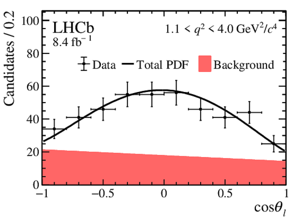
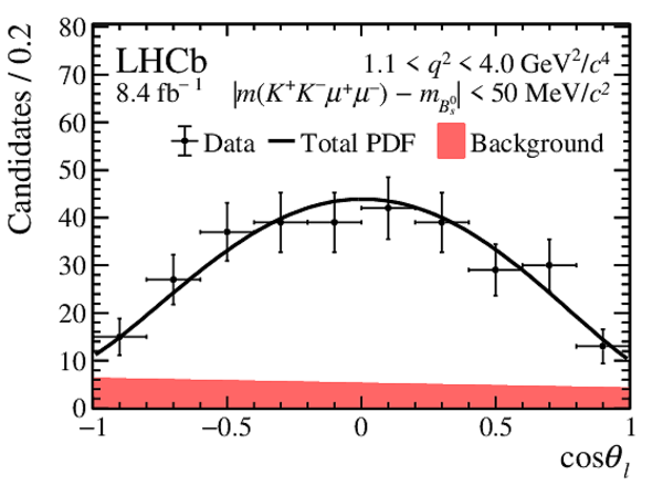
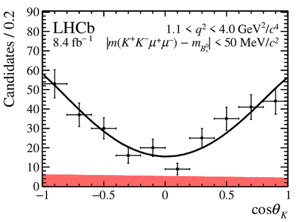
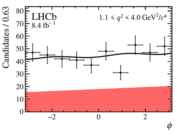
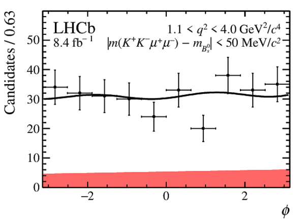
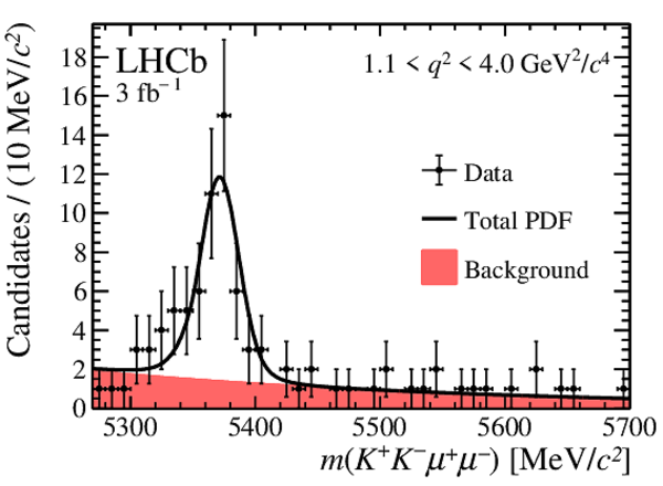
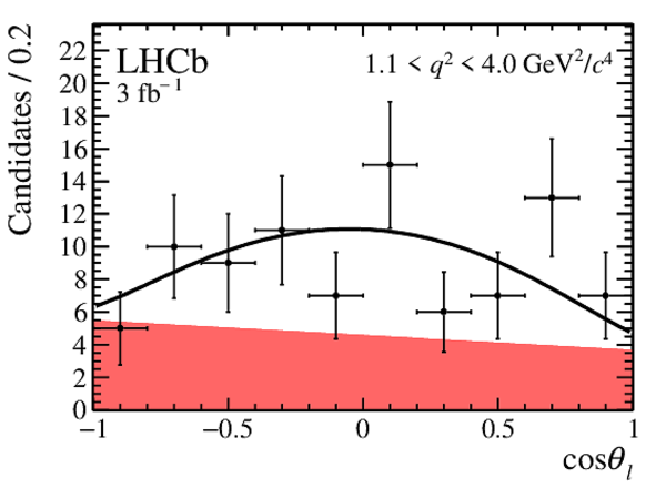
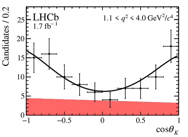
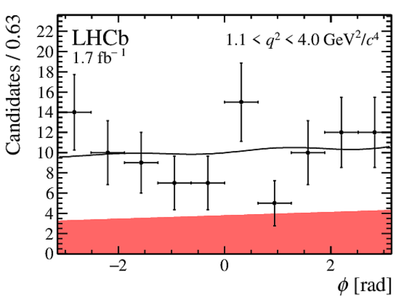
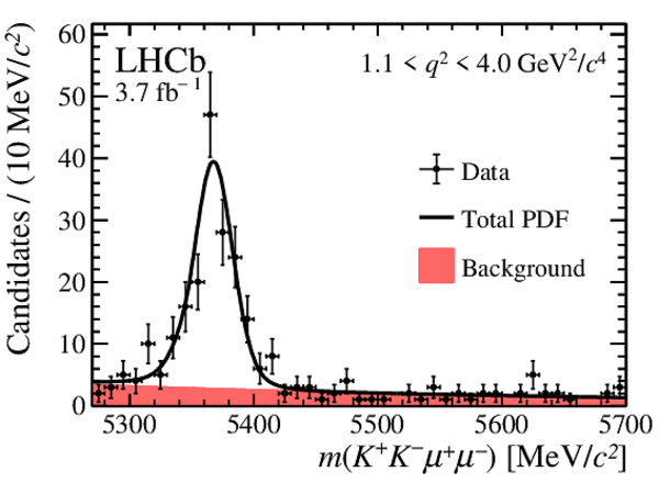
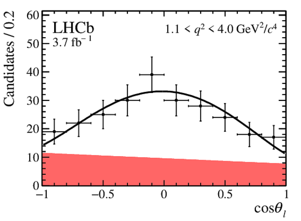
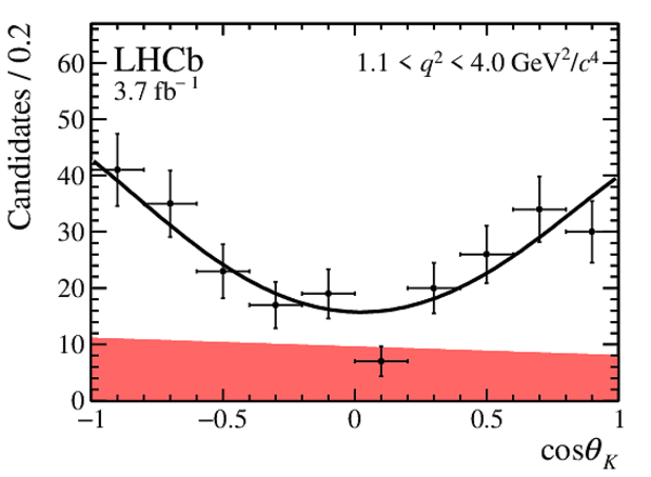
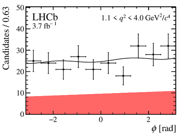
Projections in the region $1.1 < q^2 <4.0\text{ Ge V} ^2 /c^4 $ for the angular distributions of the combined 2011--2012, 2016 and 2017--2018 data set. The data are overlaid with the projection of the combined PDF. The red shaded area indicates the background component and the solid black line the total PDF. The angular projections are given for candidates in (left) the entire mass region used to determine the observables in this paper and (right) the signal mass window $\pm50\text{ Me V /}c^2 $ around the known $ B ^0_ s $ mass. |
Fig6a.pdf [13 KiB] HiDef png [155 KiB] Thumbnail [157 KiB] *.C file |
|
|
Fig6d.pdf [15 KiB] HiDef png [183 KiB] Thumbnail [193 KiB] *.C file |
|
|
|
Fig6b.pdf [12 KiB] HiDef png [134 KiB] Thumbnail [136 KiB] *.C file |

|
|
|
Fig6e.pdf [13 KiB] HiDef png [167 KiB] Thumbnail [178 KiB] *.C file |
|
|
|
Fig6c.pdf [11 KiB] HiDef png [132 KiB] Thumbnail [135 KiB] *.C file |
|
|
|
Fig6f.pdf [12 KiB] HiDef png [140 KiB] Thumbnail [141 KiB] *.C file |
|
|
|
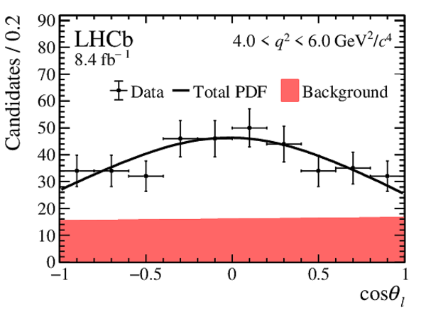
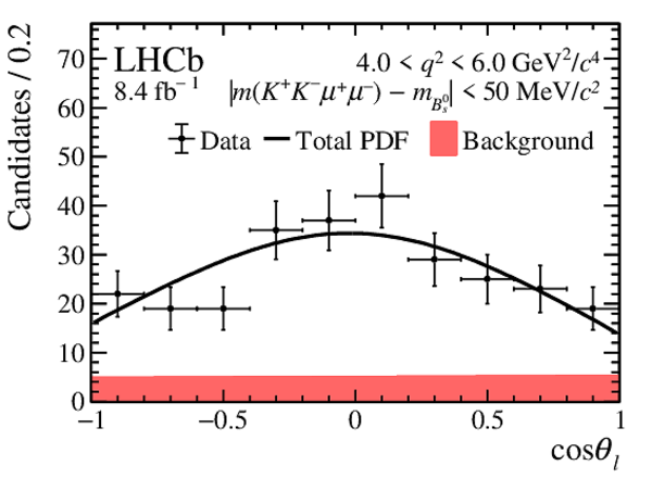
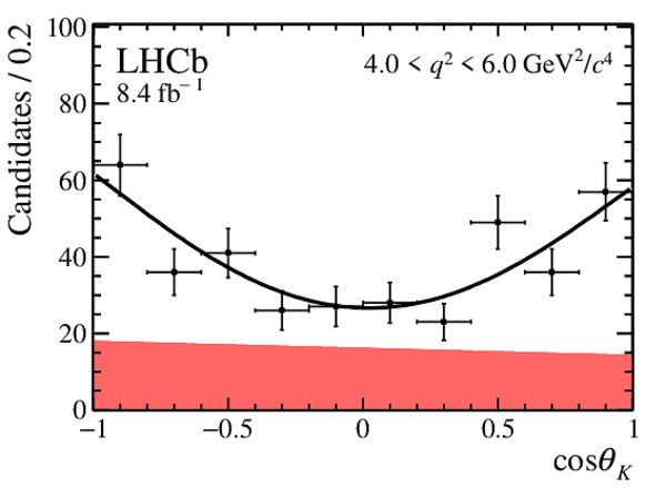
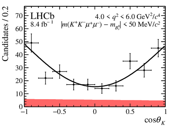
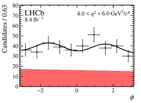
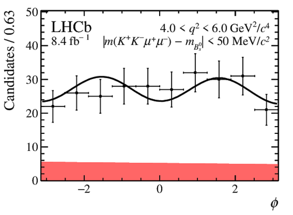
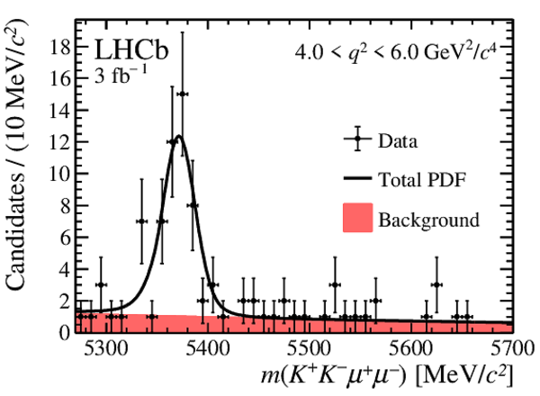
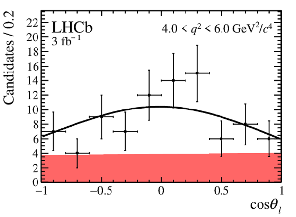
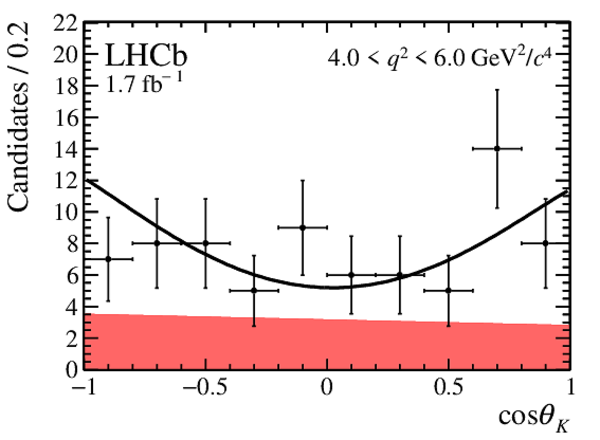
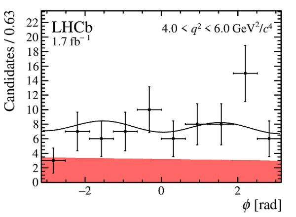
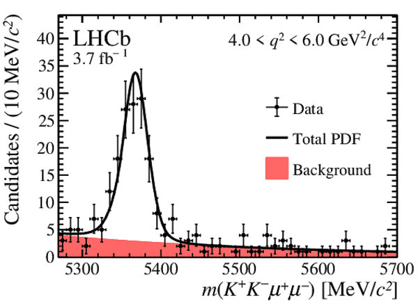
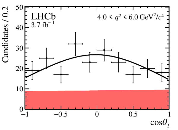
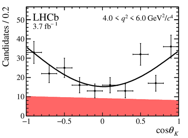
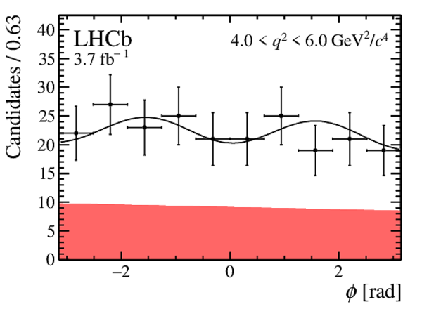
Projections in the region $4.0 < q^2 <6.0\text{ Ge V} ^2 /c^4 $ for the angular distributions of the combined 2011--2012, 2016 and 2017--2018 data sets. The data are overlaid with the projection of the combined PDF. The red shaded area indicates the background component and the solid black line the total PDF. The angular projections are given for candidates in (left) the entire mass region used to determine the observables in this paper and (right) the signal mass window $\pm50\text{ Me V /}c^2 $ around the known $ B ^0_ s $ mass. |
Fig7a.pdf [13 KiB] HiDef png [165 KiB] Thumbnail [170 KiB] *.C file |
|
|
Fig7d.pdf [14 KiB] HiDef png [178 KiB] Thumbnail [186 KiB] *.C file |
|
|
|
Fig7b.pdf [12 KiB] HiDef png [133 KiB] Thumbnail [135 KiB] *.C file |
|
|
|
Fig7e.pdf [13 KiB] HiDef png [161 KiB] Thumbnail [170 KiB] *.C file |
|
|
|
Fig7c.pdf [11 KiB] HiDef png [131 KiB] Thumbnail [138 KiB] *.C file |
|
|
|
Fig7f.pdf [12 KiB] HiDef png [144 KiB] Thumbnail [148 KiB] *.C file |
|
|
|
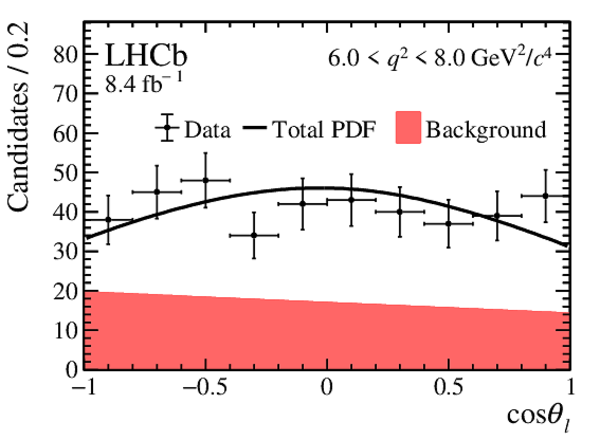
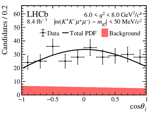
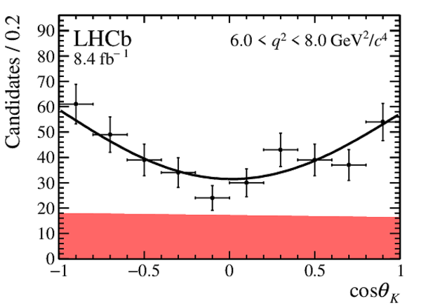
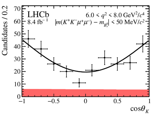
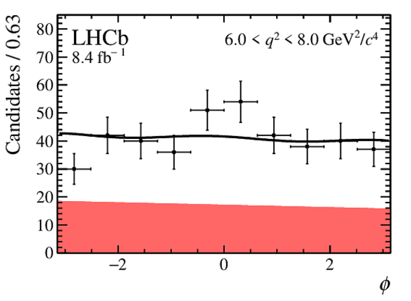
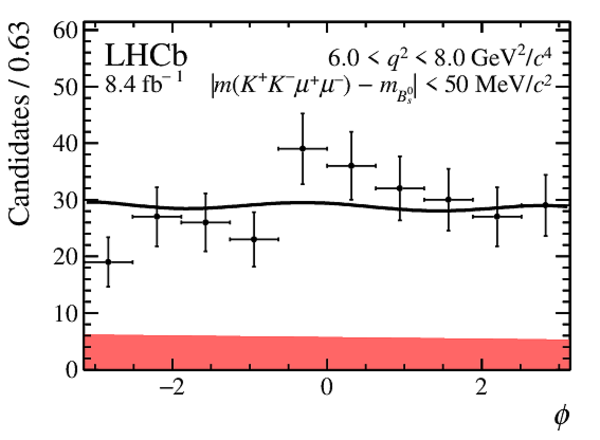
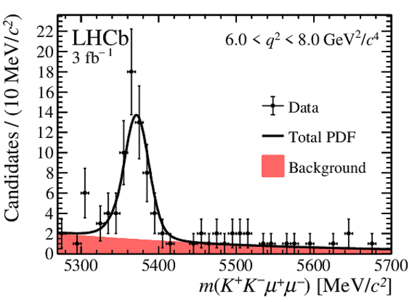
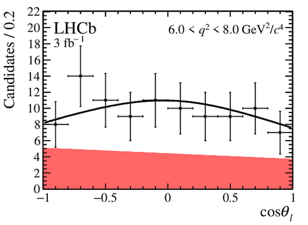
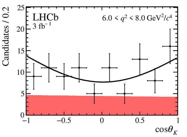
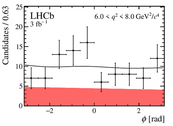
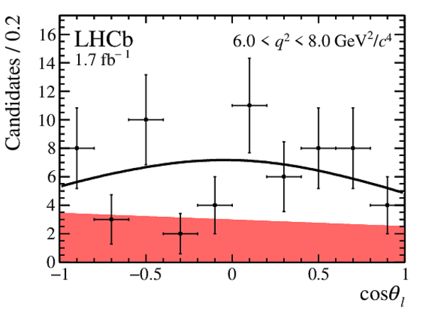
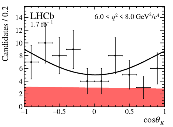
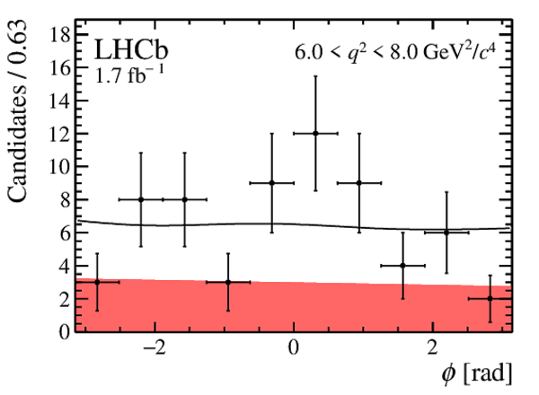
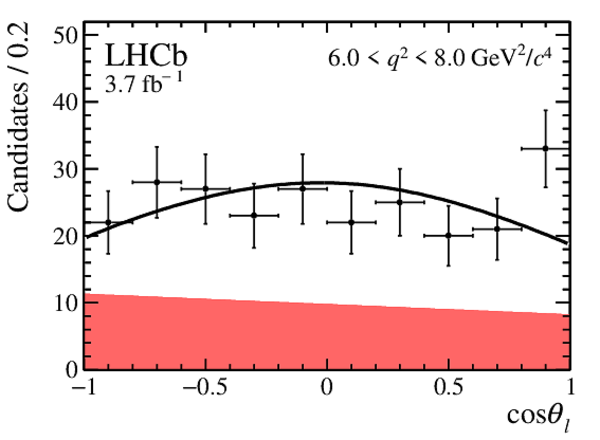
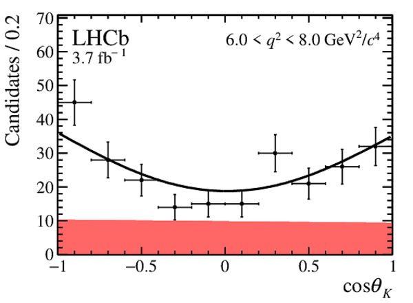
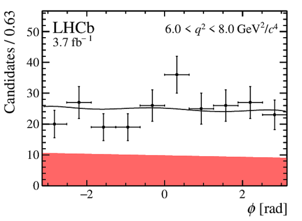
Projections in the region $6.0 < q^2 <8.0\text{ Ge V} ^2 /c^4 $ for the angular distributions of the combined 2011--2012, 2016 and 2017--2018 data sets. The data are overlaid with the projection of the combined PDF. The red shaded area indicates the background component and the solid black line the total PDF. The angular projections are given for candidates in (left) the entire mass region used to determine the observables in this paper and (right) the signal mass window $\pm50\text{ Me V /}c^2 $ around the known $ B ^0_ s $ mass. |
Fig8a.pdf [13 KiB] HiDef png [168 KiB] Thumbnail [172 KiB] *.C file |
|
|
Fig8d.pdf [14 KiB] HiDef png [177 KiB] Thumbnail [182 KiB] *.C file |
|
|
|
Fig8b.pdf [12 KiB] HiDef png [147 KiB] Thumbnail [154 KiB] *.C file |
|
|
|
Fig8e.pdf [13 KiB] HiDef png [160 KiB] Thumbnail [167 KiB] *.C file |
|
|
|
Fig8c.pdf [11 KiB] HiDef png [130 KiB] Thumbnail [133 KiB] *.C file |
|
|
|
Fig8f.pdf [12 KiB] HiDef png [144 KiB] Thumbnail [143 KiB] *.C file |
|
|
|
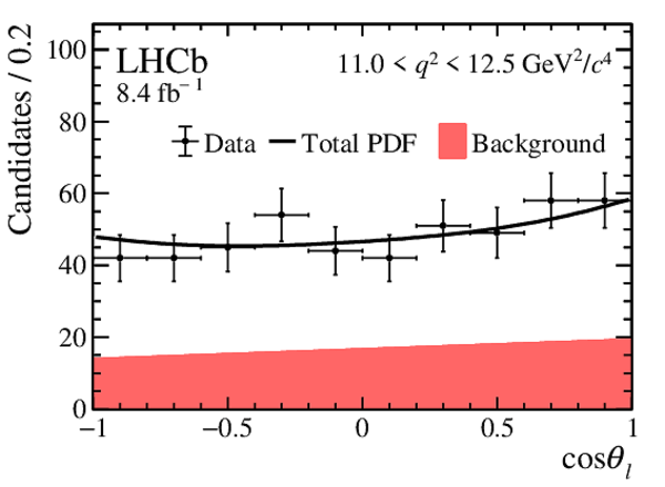
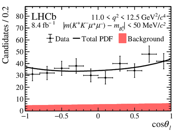
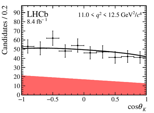
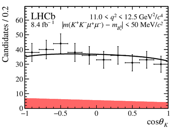
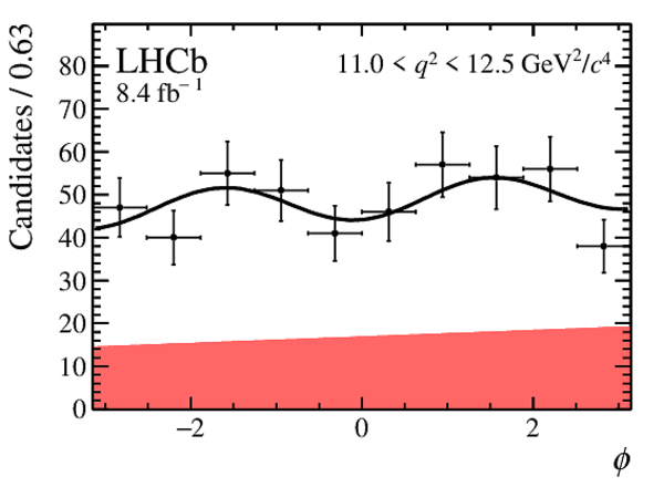
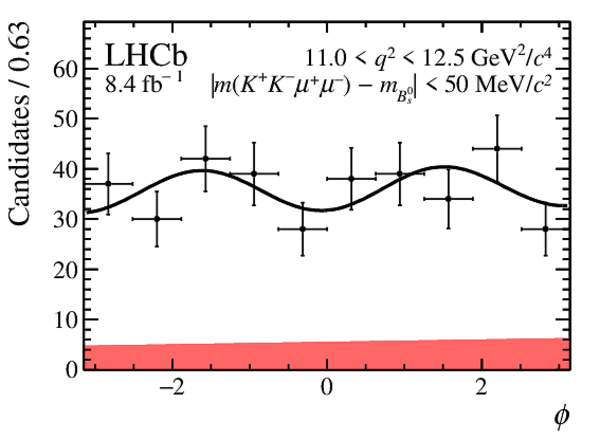
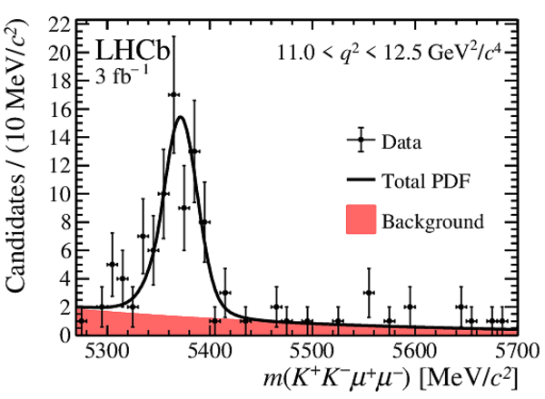
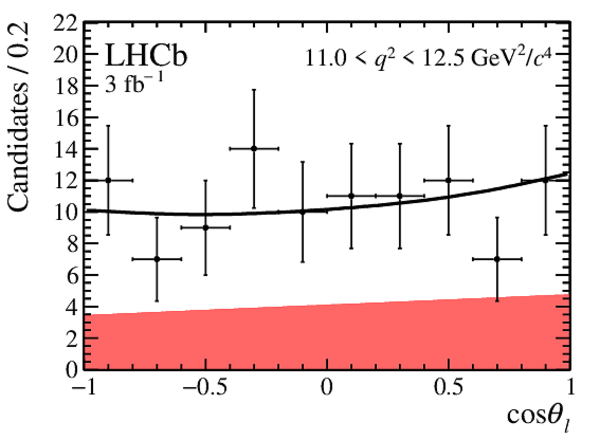
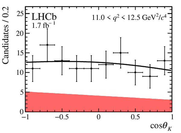
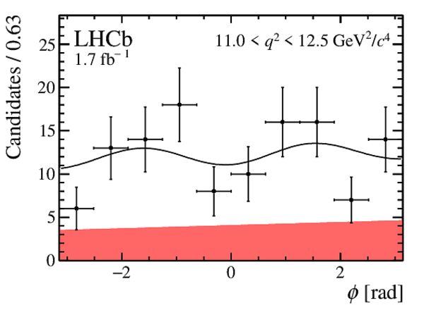
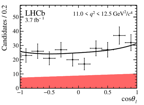
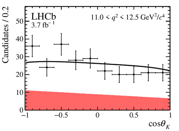
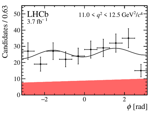
Projections in the region $11.0 < q^2 <12.5\text{ Ge V} ^2 /c^4 $ for the angular distributions of the combined 2011--2012, 2016 and 2017--2018 data sets. The data are overlaid with the projection of the combined PDF. The red shaded area indicates the background component and the solid black line the total PDF. The angular projections are given for candidates in (left) the entire mass region used to determine the observables in this paper and (right) the signal mass window $\pm50\text{ Me V /}c^2 $ around the known $ B ^0_ s $ mass. |
Fig9a.pdf [13 KiB] HiDef png [151 KiB] Thumbnail [150 KiB] *.C file |
|
|
Fig9d.pdf [14 KiB] HiDef png [181 KiB] Thumbnail [186 KiB] *.C file |
|
|
|
Fig9b.pdf [12 KiB] HiDef png [148 KiB] Thumbnail [152 KiB] *.C file |
|
|
|
Fig9e.pdf [13 KiB] HiDef png [154 KiB] Thumbnail [157 KiB] *.C file |
|
|
|
Fig9c.pdf [12 KiB] HiDef png [136 KiB] Thumbnail [143 KiB] *.C file |
|
|
|
Fig9f.pdf [13 KiB] HiDef png [148 KiB] Thumbnail [153 KiB] *.C file |
|
|
|
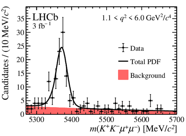
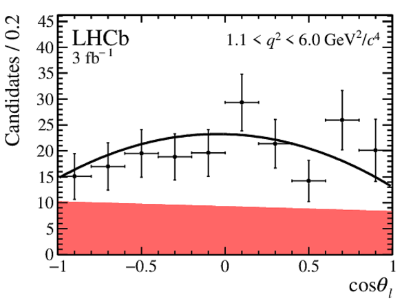
Projections in the region $1.1 < q^2 <6.0\text{ Ge V} ^2 /c^4 $ for the angular distributions of the combined 2011--2012, 2016 and 2017--2018 data sets. The data are overlaid with the projection of the combined PDF. The red shaded area indicates the background component and the solid black line the total PDF. The angular projections are given for candidates in (left) the entire mass region used to determine the observables in this paper and (right) the signal mass window $\pm50\text{ Me V /}c^2 $ around the known $ B ^0_ s $ mass. |
Fig10a.pdf [13 KiB] HiDef png [168 KiB] Thumbnail [174 KiB] *.C file |
|
|
Fig10d.pdf [14 KiB] HiDef png [178 KiB] Thumbnail [183 KiB] *.C file |

|
|
|
Fig10b.pdf [12 KiB] HiDef png [137 KiB] Thumbnail [141 KiB] *.C file |
|
|
|
Fig10e.pdf [13 KiB] HiDef png [169 KiB] Thumbnail [178 KiB] *.C file |

|
|
|
Fig10c.pdf [11 KiB] HiDef png [132 KiB] Thumbnail [133 KiB] *.C file |
|
|
|
Fig10f.pdf [12 KiB] HiDef png [141 KiB] Thumbnail [141 KiB] *.C file |
|
|
|
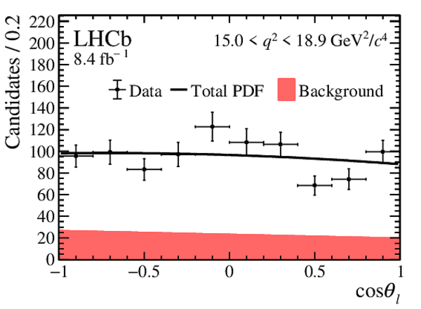
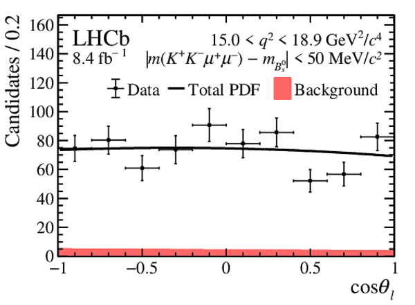
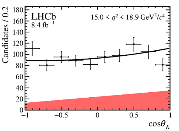
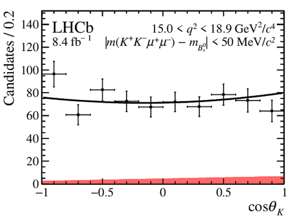
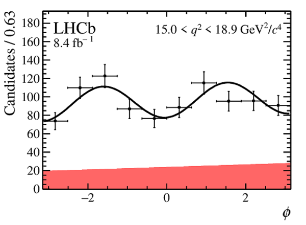
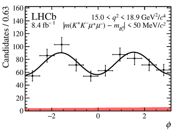
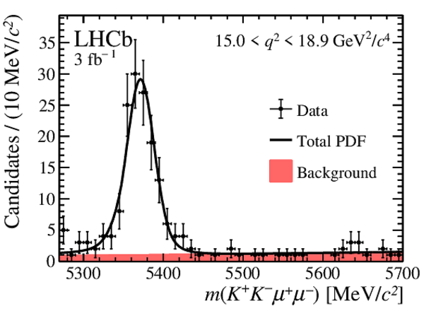
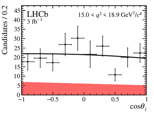
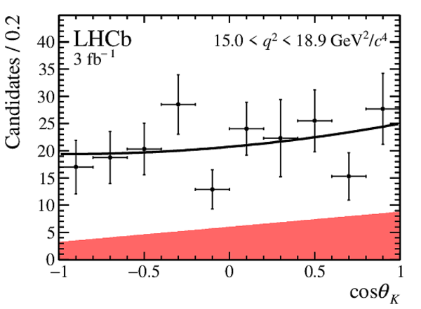
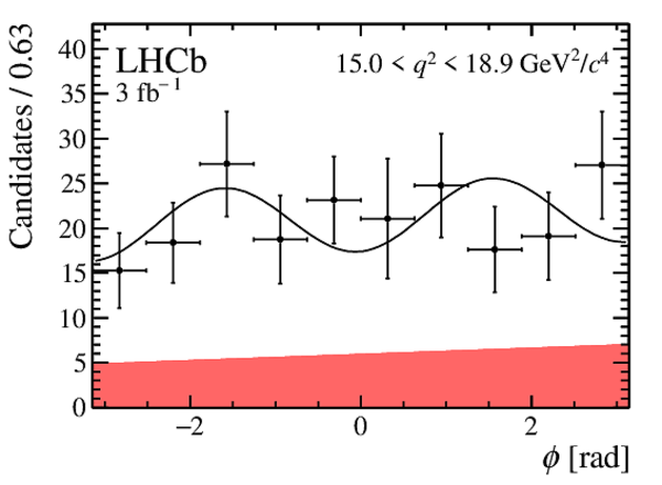
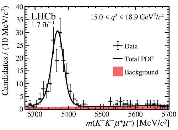
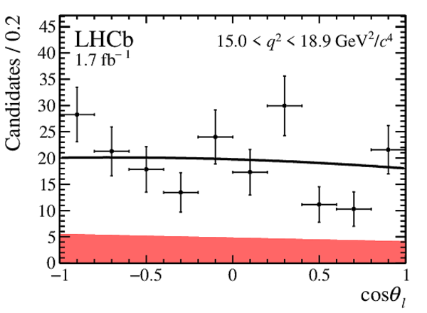
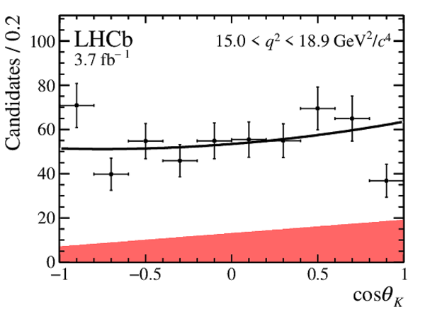
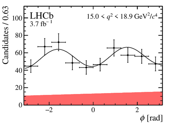
Projections in the region $15.0 < q^2 <18.9\text{ Ge V} ^2 /c^4 $ for the angular distributions of the combined 2011--2012, 2016 and 2017--2018 data sets. The data are overlaid with the projection of the combined PDF. The red shaded area indicates the background component and the solid black line the total PDF. The angular projections are given for candidates in (left) the entire mass region used to determine the observables in this paper and (right) the signal mass window $\pm50\text{ Me V /}c^2 $ around the known $ B ^0_ s $ mass. |
Fig11a.pdf [13 KiB] HiDef png [169 KiB] Thumbnail [173 KiB] *.C file |
|
|
Fig11d.pdf [14 KiB] HiDef png [175 KiB] Thumbnail [178 KiB] *.C file |
|
|
|
Fig11b.pdf [12 KiB] HiDef png [147 KiB] Thumbnail [149 KiB] *.C file |
|
|
|
Fig11e.pdf [13 KiB] HiDef png [156 KiB] Thumbnail [158 KiB] *.C file |
|
|
|
Fig11c.pdf [12 KiB] HiDef png [142 KiB] Thumbnail [150 KiB] *.C file |
|
|
|
Fig11f.pdf [13 KiB] HiDef png [156 KiB] Thumbnail [163 KiB] *.C file |
|
|
|
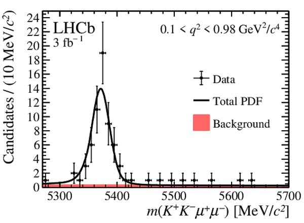
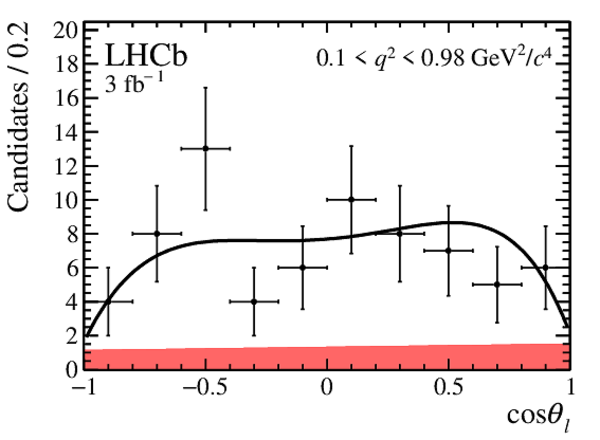
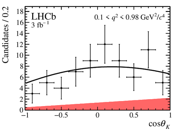
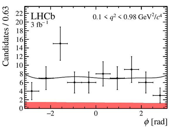
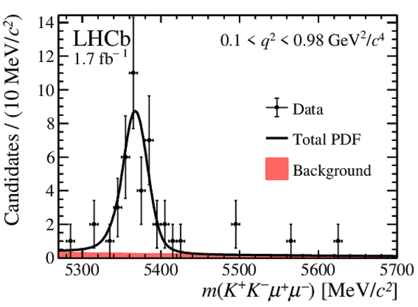
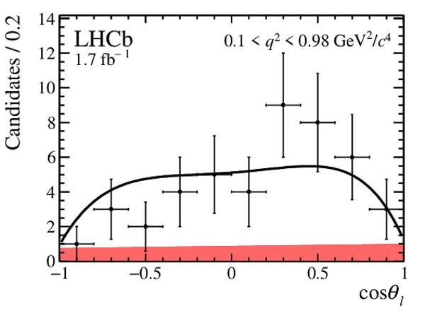
Mass and angular distributions of $ B ^0_ s \rightarrow \phi\mu ^+ \mu ^- $ candidates in the region $0.1< q^2 <0.98\text{ Ge V} ^2 /c^4 $ for data taken in 2011--2012. The data are overlaid with the projections of the fitted PDF. |
Fig12a.pdf [16 KiB] HiDef png [209 KiB] Thumbnail [213 KiB] *.C file |
|
|
Fig12b.pdf [11 KiB] HiDef png [137 KiB] Thumbnail [142 KiB] *.C file |
|
|
|
Fig12c.pdf [12 KiB] HiDef png [139 KiB] Thumbnail [142 KiB] *.C file |
|
|
|
Fig12d.pdf [11 KiB] HiDef png [130 KiB] Thumbnail [131 KiB] *.C file |
|
|
|
Mass and angular distributions of $ B ^0_ s \rightarrow \phi\mu ^+ \mu ^- $ candidates in the region $0.1< q^2 <0.98\text{ Ge V} ^2 /c^4 $ for data taken in 2016. The data are overlaid with the projections of the fitted PDF. |
Fig13a.pdf [15 KiB] HiDef png [196 KiB] Thumbnail [193 KiB] *.C file |
|
|
Fig13b.pdf [11 KiB] HiDef png [131 KiB] Thumbnail [133 KiB] *.C file |
|
|
|
Fig13c.pdf [12 KiB] HiDef png [132 KiB] Thumbnail [130 KiB] *.C file |
|
|
|
Fig13d.pdf [11 KiB] HiDef png [121 KiB] Thumbnail [116 KiB] *.C file |
|
|
|
Mass and angular distributions of $ B ^0_ s \rightarrow \phi\mu ^+ \mu ^- $ candidates in the region $0.1< q^2 <0.98\text{ Ge V} ^2 /c^4 $ for data taken in 2017--2018. The data are overlaid with the projections of the fitted PDF. |
Fig14a.pdf [16 KiB] HiDef png [208 KiB] Thumbnail [209 KiB] *.C file |
|
|
Fig14b.pdf [11 KiB] HiDef png [138 KiB] Thumbnail [143 KiB] *.C file |
|
|
|
Fig14c.pdf [12 KiB] HiDef png [137 KiB] Thumbnail [140 KiB] *.C file |
|
|
|
Fig14d.pdf [11 KiB] HiDef png [126 KiB] Thumbnail [128 KiB] *.C file |
|
|
|
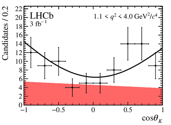
Mass and angular distributions of $ B ^0_ s \rightarrow \phi\mu ^+ \mu ^- $ candidates in the region $1.1< q^2 <4.0\text{ Ge V} ^2 /c^4 $ for data taken in 2011--2012. The data are overlaid with the projections of the fitted PDF. |
Fig15a.pdf [17 KiB] HiDef png [223 KiB] Thumbnail [221 KiB] *.C file |
|
|
Fig15b.pdf [12 KiB] HiDef png [146 KiB] Thumbnail [151 KiB] *.C file |
|
|
|
Fig15c.pdf [12 KiB] HiDef png [149 KiB] Thumbnail [153 KiB] *.C file |
|
|
|
Fig15d.pdf [11 KiB] HiDef png [130 KiB] Thumbnail [128 KiB] *.C file |
|
|
|
Mass and angular distributions of $ B ^0_ s \rightarrow \phi\mu ^+ \mu ^- $ candidates in the region $1.1< q^2 <4.0\text{ Ge V} ^2 /c^4 $ for data taken in 2016. The data are overlaid with the projections of the fitted PDF. |
Fig16a.pdf [16 KiB] HiDef png [218 KiB] Thumbnail [222 KiB] *.C file |
|
|
Fig16b.pdf [12 KiB] HiDef png [147 KiB] Thumbnail [154 KiB] *.C file |
|
|
|
Fig16c.pdf [11 KiB] HiDef png [132 KiB] Thumbnail [136 KiB] *.C file |
|
|
|
Fig16d.pdf [11 KiB] HiDef png [133 KiB] Thumbnail [134 KiB] *.C file |
|
|
|
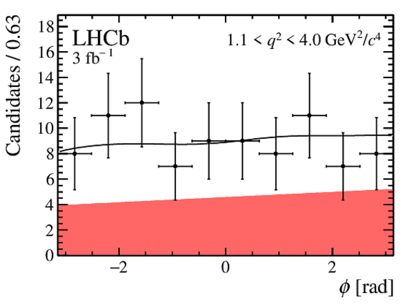
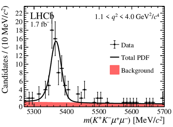
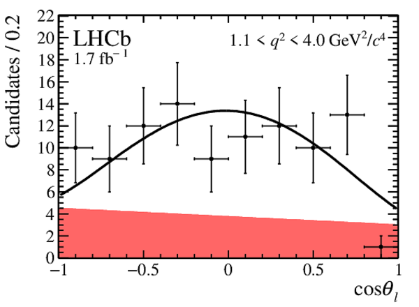
Mass and angular distributions of $ B ^0_ s \rightarrow \phi\mu ^+ \mu ^- $ candidates in the region $1.1< q^2 <4.0\text{ Ge V} ^2 /c^4 $ for data taken in 2017--2018. The data are overlaid with the projections of the fitted PDF. |
Fig17a.pdf [18 KiB] HiDef png [227 KiB] Thumbnail [216 KiB] *.C file |
|
|
Fig17b.pdf [12 KiB] HiDef png [136 KiB] Thumbnail [142 KiB] *.C file |
|
|
|
Fig17c.pdf [12 KiB] HiDef png [139 KiB] Thumbnail [144 KiB] *.C file |
|
|
|
Fig17d.pdf [11 KiB] HiDef png [125 KiB] Thumbnail [122 KiB] *.C file |
|
|
|
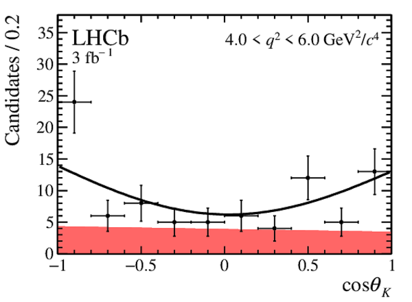
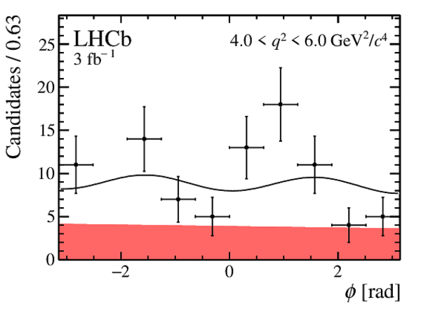
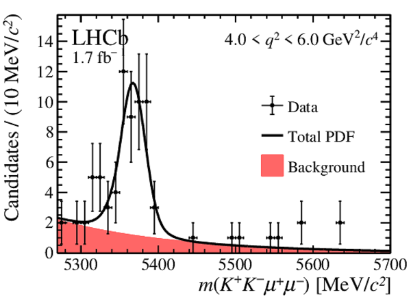
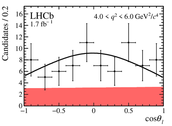
Mass and angular distributions of $ B ^0_ s \rightarrow \phi\mu ^+ \mu ^- $ candidates in the region $4.0< q^2 <6.0\text{ Ge V} ^2 /c^4 $ for data taken in 2011--2012. The data are overlaid with the projections of the fitted PDF. |
Fig18a.pdf [17 KiB] HiDef png [222 KiB] Thumbnail [221 KiB] *.C file |
|
|
Fig18b.pdf [12 KiB] HiDef png [140 KiB] Thumbnail [145 KiB] *.C file |
|
|
|
Fig18c.pdf [11 KiB] HiDef png [134 KiB] Thumbnail [140 KiB] *.C file |
|
|
|
Fig18d.pdf [11 KiB] HiDef png [122 KiB] Thumbnail [122 KiB] *.C file |
|
|
|
Mass and angular distributions of $ B ^0_ s \rightarrow \phi\mu ^+ \mu ^- $ candidates in the region $4.0< q^2 <6.0\text{ Ge V} ^2 /c^4 $ for data taken in 2016. The data are overlaid with the projections of the fitted PDF. |
Fig19a.pdf [17 KiB] HiDef png [211 KiB] Thumbnail [207 KiB] *.C file |
|
|
Fig19b.pdf [11 KiB] HiDef png [134 KiB] Thumbnail [137 KiB] *.C file |
|
|
|
Fig19c.pdf [12 KiB] HiDef png [144 KiB] Thumbnail [151 KiB] *.C file |
|
|
|
Fig19d.pdf [11 KiB] HiDef png [136 KiB] Thumbnail [138 KiB] *.C file |
|
|
|
Mass and angular distributions of $ B ^0_ s \rightarrow \phi\mu ^+ \mu ^- $ candidates in the region $4.0< q^2 <6.0\text{ Ge V} ^2 /c^4 $ for data taken in 2017--2018. The data are overlaid with the projections of the fitted PDF. |
Fig20a.pdf [18 KiB] HiDef png [241 KiB] Thumbnail [235 KiB] *.C file |
|
|
Fig20b.pdf [11 KiB] HiDef png [129 KiB] Thumbnail [132 KiB] *.C file |
|
|
|
Fig20c.pdf [12 KiB] HiDef png [134 KiB] Thumbnail [140 KiB] *.C file |
|
|
|
Fig20d.pdf [11 KiB] HiDef png [136 KiB] Thumbnail [140 KiB] *.C file |
|
|
|
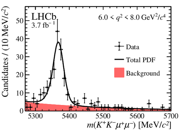
Mass and angular distributions of $ B ^0_ s \rightarrow \phi\mu ^+ \mu ^- $ candidates in the region $6.0< q^2 <8.0\text{ Ge V} ^2 /c^4 $ for data taken in 2011--2012. The data are overlaid with the projections of the fitted PDF. |
Fig21a.pdf [17 KiB] HiDef png [226 KiB] Thumbnail [225 KiB] *.C file |
|
|
Fig21b.pdf [12 KiB] HiDef png [145 KiB] Thumbnail [150 KiB] *.C file |
|
|
|
Fig21c.pdf [11 KiB] HiDef png [130 KiB] Thumbnail [129 KiB] *.C file |
|
|
|
Fig21d.pdf [11 KiB] HiDef png [120 KiB] Thumbnail [116 KiB] *.C file |
|
|
|
Mass and angular distributions of $ B ^0_ s \rightarrow \phi\mu ^+ \mu ^- $ candidates in the region $6.0< q^2 <8.0\text{ Ge V} ^2 /c^4 $ for data taken in 2016. The data are overlaid with the projections of the fitted PDF. |
Fig22a.pdf [17 KiB] HiDef png [215 KiB] Thumbnail [210 KiB] *.C file |
|
|
Fig22b.pdf [12 KiB] HiDef png [138 KiB] Thumbnail [139 KiB] *.C file |
|
|
|
Fig22c.pdf [11 KiB] HiDef png [135 KiB] Thumbnail [137 KiB] *.C file |
|
|
|
Fig22d.pdf [11 KiB] HiDef png [128 KiB] Thumbnail [127 KiB] *.C file |
|
|
|
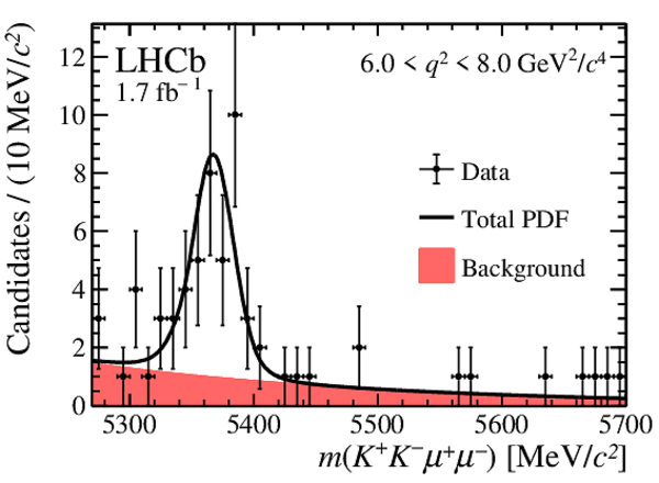
Mass and angular distributions of $ B ^0_ s \rightarrow \phi\mu ^+ \mu ^- $ candidates in the region $6.0< q^2 <8.0\text{ Ge V} ^2 /c^4 $ for data taken in 2017--2018. The data are overlaid with the projections of the fitted PDF. |
Fig23a.pdf [18 KiB] HiDef png [223 KiB] Thumbnail [215 KiB] *.C file |
|
|
Fig23b.pdf [12 KiB] HiDef png [134 KiB] Thumbnail [136 KiB] *.C file |
|
|
|
Fig23c.pdf [12 KiB] HiDef png [136 KiB] Thumbnail [142 KiB] *.C file |
|
|
|
Fig23d.pdf [11 KiB] HiDef png [124 KiB] Thumbnail [123 KiB] *.C file |
|
|
|
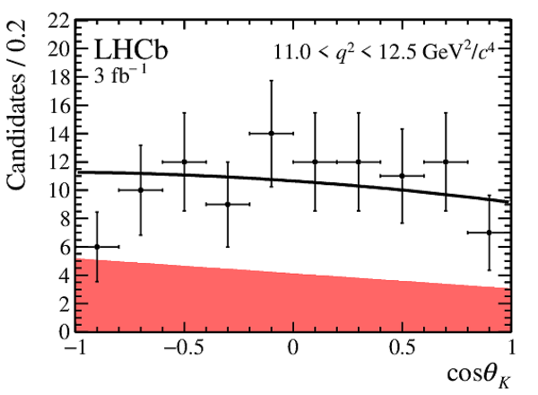
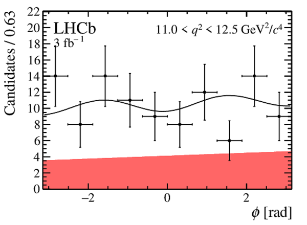
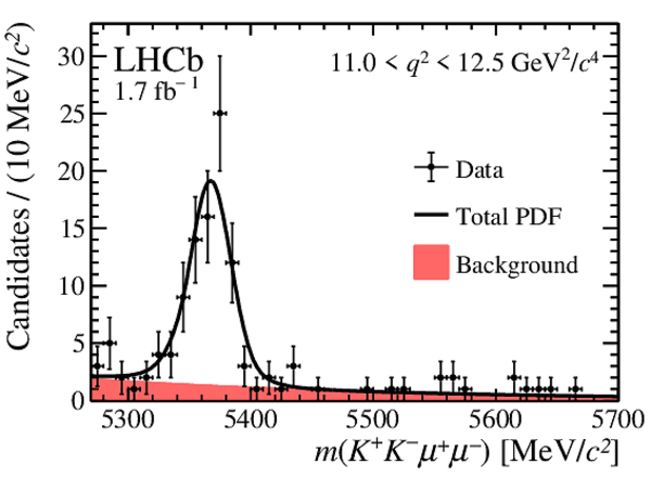
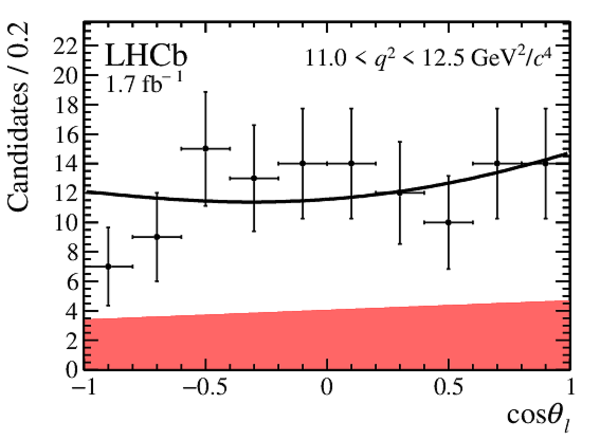
Mass and angular distributions of $ B ^0_ s \rightarrow \phi\mu ^+ \mu ^- $ candidates in the region $11.0< q^2 <12.5\text{ Ge V} ^2 /c^4 $ for data taken in 2011--2012. The data are overlaid with the projections of the fitted PDF. |
Fig24a.pdf [17 KiB] HiDef png [225 KiB] Thumbnail [225 KiB] *.C file |
|
|
Fig24b.pdf [12 KiB] HiDef png [142 KiB] Thumbnail [143 KiB] *.C file |
|
|
|
Fig24c.pdf [12 KiB] HiDef png [145 KiB] Thumbnail [148 KiB] *.C file |
|
|
|
Fig24d.pdf [12 KiB] HiDef png [140 KiB] Thumbnail [142 KiB] *.C file |
|
|
|
Mass and angular distributions of $ B ^0_ s \rightarrow \phi\mu ^+ \mu ^- $ candidates in the region $11.0< q^2 <12.5\text{ Ge V} ^2 /c^4 $ for data taken in 2016. The data are overlaid with the projections of the fitted PDF. |
Fig25a.pdf [17 KiB] HiDef png [212 KiB] Thumbnail [211 KiB] *.C file |
|
|
Fig25b.pdf [12 KiB] HiDef png [143 KiB] Thumbnail [146 KiB] *.C file |
|
|
|
Fig25c.pdf [11 KiB] HiDef png [130 KiB] Thumbnail [128 KiB] *.C file |
|
|
|
Fig25d.pdf [11 KiB] HiDef png [126 KiB] Thumbnail [126 KiB] *.C file |
|
|
|
Mass and angular distributions of $ B ^0_ s \rightarrow \phi\mu ^+ \mu ^- $ candidates in the region $11.0< q^2 <12.5\text{ Ge V} ^2 /c^4 $ for data taken in 2017--2018. The data are overlaid with the projections of the fitted PDF. |
Fig26a.pdf [18 KiB] HiDef png [223 KiB] Thumbnail [216 KiB] *.C file |
|
|
Fig26b.pdf [11 KiB] HiDef png [131 KiB] Thumbnail [131 KiB] *.C file |
|
|
|
Fig26c.pdf [12 KiB] HiDef png [133 KiB] Thumbnail [133 KiB] *.C file |
|
|
|
Fig26d.pdf [11 KiB] HiDef png [127 KiB] Thumbnail [127 KiB] *.C file |
|
|
|
Mass and angular distributions of $ B ^0_ s \rightarrow \phi\mu ^+ \mu ^- $ candidates in the region $1.1< q^2 <6.0\text{ Ge V} ^2 /c^4 $ for data taken in 2011--2012. The data are overlaid with the projections of the fitted PDF. |
Fig27a.pdf [18 KiB] HiDef png [232 KiB] Thumbnail [225 KiB] *.C file |
|
|
Fig27b.pdf [12 KiB] HiDef png [141 KiB] Thumbnail [149 KiB] *.C file |
|
|
|
Fig27c.pdf [12 KiB] HiDef png [136 KiB] Thumbnail [142 KiB] *.C file |
|
|
|
Fig27d.pdf [11 KiB] HiDef png [135 KiB] Thumbnail [137 KiB] *.C file |
|
|
|
Mass and angular distributions of $ B ^0_ s \rightarrow \phi\mu ^+ \mu ^- $ candidates in the region $1.1< q^2 <6.0\text{ Ge V} ^2 /c^4 $ for data taken in 2016. The data are overlaid with the projections of the fitted PDF. |
Fig28a.pdf [17 KiB] HiDef png [223 KiB] Thumbnail [220 KiB] *.C file |
|
|
Fig28b.pdf [12 KiB] HiDef png [140 KiB] Thumbnail [146 KiB] *.C file |
|
|
|
Fig28c.pdf [12 KiB] HiDef png [135 KiB] Thumbnail [138 KiB] *.C file |
|
|
|
Fig28d.pdf [11 KiB] HiDef png [134 KiB] Thumbnail [138 KiB] *.C file |
|
|
|
Mass and angular distributions of $ B ^0_ s \rightarrow \phi\mu ^+ \mu ^- $ candidates in the region $1.1< q^2 <6.0\text{ Ge V} ^2 /c^4 $ for data taken in 2017--2018. The data are overlaid with the projections of the fitted PDF. |
Fig29a.pdf [19 KiB] HiDef png [244 KiB] Thumbnail [236 KiB] *.C file |
|
|
Fig29b.pdf [12 KiB] HiDef png [148 KiB] Thumbnail [155 KiB] *.C file |
|
|
|
Fig29c.pdf [12 KiB] HiDef png [141 KiB] Thumbnail [145 KiB] *.C file |
|
|
|
Fig29d.pdf [12 KiB] HiDef png [141 KiB] Thumbnail [146 KiB] *.C file |
|
|
|
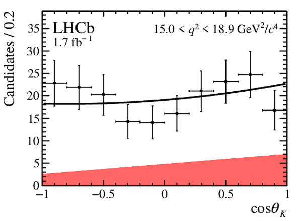
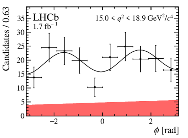
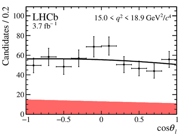
Mass and angular distributions of $ B ^0_ s \rightarrow \phi\mu ^+ \mu ^- $ candidates in the region $15.0< q^2 <18.9\text{ Ge V} ^2 /c^4 $ for data taken in 2011--2012. The data are overlaid with the projections of the fitted PDF. |
Fig30a.pdf [17 KiB] HiDef png [224 KiB] Thumbnail [220 KiB] *.C file |
|
|
Fig30b.pdf [11 KiB] HiDef png [137 KiB] Thumbnail [141 KiB] *.C file |
|
|
|
Fig30c.pdf [12 KiB] HiDef png [143 KiB] Thumbnail [147 KiB] *.C file |
|
|
|
Fig30d.pdf [12 KiB] HiDef png [140 KiB] Thumbnail [145 KiB] *.C file |
|
|
|
Mass and angular distributions of $ B ^0_ s \rightarrow \phi\mu ^+ \mu ^- $ candidates in the region $15.0< q^2 <18.9\text{ Ge V} ^2 /c^4 $ for data taken in 2016. The data are overlaid with the projections of the fitted PDF. |
Fig31a.pdf [18 KiB] HiDef png [229 KiB] Thumbnail [226 KiB] *.C file |
|
|
Fig31b.pdf [11 KiB] HiDef png [136 KiB] Thumbnail [140 KiB] *.C file |
|
|
|
Fig31c.pdf [12 KiB] HiDef png [139 KiB] Thumbnail [142 KiB] *.C file |
|
|
|
Fig31d.pdf [12 KiB] HiDef png [136 KiB] Thumbnail [140 KiB] *.C file |
|
|
|
Mass and angular distributions of $ B ^0_ s \rightarrow \phi\mu ^+ \mu ^- $ candidates in the region $15.0< q^2 <18.9\text{ Ge V} ^2 /c^4 $ for data taken in 2017--2018. The data are overlaid with the projections of the fitted PDF. |
Fig32a.pdf [18 KiB] HiDef png [223 KiB] Thumbnail [208 KiB] *.C file |
|
|
Fig32b.pdf [11 KiB] HiDef png [126 KiB] Thumbnail [124 KiB] *.C file |
|
|
|
Fig32c.pdf [12 KiB] HiDef png [133 KiB] Thumbnail [131 KiB] *.C file |
|
|
|
Fig32d.pdf [12 KiB] HiDef png [130 KiB] Thumbnail [130 KiB] *.C file |
|
|
|
Animated gif made out of all figures. |
PAPER-2021-022.gif Thumbnail |

|
![HiDef png [226 KiB]](Directory_LHCb-PAPER-2021-022/hidef_Fig1a.png)
![HiDef png [222 KiB]](Directory_LHCb-PAPER-2021-022/hidef_Fig1b.png)
![HiDef png [223 KiB]](Directory_LHCb-PAPER-2021-022/hidef_Fig1c.png)
![HiDef png [168 KiB]](Directory_LHCb-PAPER-2021-022/hidef_Fig2a.png)
![HiDef png [178 KiB]](Directory_LHCb-PAPER-2021-022/hidef_Fig2d.png)
![HiDef png [137 KiB]](Directory_LHCb-PAPER-2021-022/hidef_Fig2b.png)
![HiDef png [169 KiB]](Directory_LHCb-PAPER-2021-022/hidef_Fig2e.png)
![HiDef png [132 KiB]](Directory_LHCb-PAPER-2021-022/hidef_Fig2c.png)
![HiDef png [141 KiB]](Directory_LHCb-PAPER-2021-022/hidef_Fig2f.png)
![HiDef png [220 KiB]](Directory_LHCb-PAPER-2021-022/hidef_Fig3a.png)
![HiDef png [212 KiB]](Directory_LHCb-PAPER-2021-022/hidef_Fig3b.png)
![HiDef png [212 KiB]](Directory_LHCb-PAPER-2021-022/hidef_Fig3c.png)
![HiDef png [214 KiB]](Directory_LHCb-PAPER-2021-022/hidef_Fig3d.png)
![HiDef png [150 KiB]](Directory_LHCb-PAPER-2021-022/hidef_Fig3e.png)
![HiDef png [152 KiB]](Directory_LHCb-PAPER-2021-022/hidef_Fig3f.png)
![HiDef png [150 KiB]](Directory_LHCb-PAPER-2021-022/hidef_Fig3g.png)
![HiDef png [149 KiB]](Directory_LHCb-PAPER-2021-022/hidef_Fig3h.png)
![HiDef png [210 KiB]](Directory_LHCb-PAPER-2021-022/hidef_Fig4a.png)
![HiDef png [238 KiB]](Directory_LHCb-PAPER-2021-022/hidef_Fig4b.png)
![HiDef png [241 KiB]](Directory_LHCb-PAPER-2021-022/hidef_Fig4c.png)
![HiDef png [239 KiB]](Directory_LHCb-PAPER-2021-022/hidef_Fig4d.png)
![HiDef png [223 KiB]](Directory_LHCb-PAPER-2021-022/hidef_Fig4e.png)
![HiDef png [239 KiB]](Directory_LHCb-PAPER-2021-022/hidef_Fig4f.png)
![HiDef png [235 KiB]](Directory_LHCb-PAPER-2021-022/hidef_Fig4g.png)
![HiDef png [158 KiB]](Directory_LHCb-PAPER-2021-022/hidef_Fig5a.png)
![HiDef png [177 KiB]](Directory_LHCb-PAPER-2021-022/hidef_Fig5d.png)
![HiDef png [137 KiB]](Directory_LHCb-PAPER-2021-022/hidef_Fig5b.png)
![HiDef png [152 KiB]](Directory_LHCb-PAPER-2021-022/hidef_Fig5e.png)
![HiDef png [119 KiB]](Directory_LHCb-PAPER-2021-022/hidef_Fig5c.png)
![HiDef png [140 KiB]](Directory_LHCb-PAPER-2021-022/hidef_Fig5f.png)
![HiDef png [155 KiB]](Directory_LHCb-PAPER-2021-022/hidef_Fig6a.png)
![HiDef png [183 KiB]](Directory_LHCb-PAPER-2021-022/hidef_Fig6d.png)
![HiDef png [134 KiB]](Directory_LHCb-PAPER-2021-022/hidef_Fig6b.png)
![HiDef png [167 KiB]](Directory_LHCb-PAPER-2021-022/hidef_Fig6e.png)
![HiDef png [132 KiB]](Directory_LHCb-PAPER-2021-022/hidef_Fig6c.png)
![HiDef png [140 KiB]](Directory_LHCb-PAPER-2021-022/hidef_Fig6f.png)
![HiDef png [165 KiB]](Directory_LHCb-PAPER-2021-022/hidef_Fig7a.png)
![HiDef png [178 KiB]](Directory_LHCb-PAPER-2021-022/hidef_Fig7d.png)
![HiDef png [133 KiB]](Directory_LHCb-PAPER-2021-022/hidef_Fig7b.png)
![HiDef png [161 KiB]](Directory_LHCb-PAPER-2021-022/hidef_Fig7e.png)
![HiDef png [131 KiB]](Directory_LHCb-PAPER-2021-022/hidef_Fig7c.png)
![HiDef png [144 KiB]](Directory_LHCb-PAPER-2021-022/hidef_Fig7f.png)
![HiDef png [168 KiB]](Directory_LHCb-PAPER-2021-022/hidef_Fig8a.png)
![HiDef png [177 KiB]](Directory_LHCb-PAPER-2021-022/hidef_Fig8d.png)
![HiDef png [147 KiB]](Directory_LHCb-PAPER-2021-022/hidef_Fig8b.png)
![HiDef png [160 KiB]](Directory_LHCb-PAPER-2021-022/hidef_Fig8e.png)
![HiDef png [130 KiB]](Directory_LHCb-PAPER-2021-022/hidef_Fig8c.png)
![HiDef png [144 KiB]](Directory_LHCb-PAPER-2021-022/hidef_Fig8f.png)
![HiDef png [151 KiB]](Directory_LHCb-PAPER-2021-022/hidef_Fig9a.png)
![HiDef png [181 KiB]](Directory_LHCb-PAPER-2021-022/hidef_Fig9d.png)
![HiDef png [148 KiB]](Directory_LHCb-PAPER-2021-022/hidef_Fig9b.png)
![HiDef png [154 KiB]](Directory_LHCb-PAPER-2021-022/hidef_Fig9e.png)
![HiDef png [136 KiB]](Directory_LHCb-PAPER-2021-022/hidef_Fig9c.png)
![HiDef png [148 KiB]](Directory_LHCb-PAPER-2021-022/hidef_Fig9f.png)
![HiDef png [168 KiB]](Directory_LHCb-PAPER-2021-022/hidef_Fig10a.png)
![HiDef png [178 KiB]](Directory_LHCb-PAPER-2021-022/hidef_Fig10d.png)
![HiDef png [137 KiB]](Directory_LHCb-PAPER-2021-022/hidef_Fig10b.png)
![HiDef png [169 KiB]](Directory_LHCb-PAPER-2021-022/hidef_Fig10e.png)
![HiDef png [132 KiB]](Directory_LHCb-PAPER-2021-022/hidef_Fig10c.png)
![HiDef png [141 KiB]](Directory_LHCb-PAPER-2021-022/hidef_Fig10f.png)
![HiDef png [169 KiB]](Directory_LHCb-PAPER-2021-022/hidef_Fig11a.png)
![HiDef png [175 KiB]](Directory_LHCb-PAPER-2021-022/hidef_Fig11d.png)
![HiDef png [147 KiB]](Directory_LHCb-PAPER-2021-022/hidef_Fig11b.png)
![HiDef png [156 KiB]](Directory_LHCb-PAPER-2021-022/hidef_Fig11e.png)
![HiDef png [142 KiB]](Directory_LHCb-PAPER-2021-022/hidef_Fig11c.png)
![HiDef png [156 KiB]](Directory_LHCb-PAPER-2021-022/hidef_Fig11f.png)
![HiDef png [209 KiB]](Directory_LHCb-PAPER-2021-022/hidef_Fig12a.png)
![HiDef png [137 KiB]](Directory_LHCb-PAPER-2021-022/hidef_Fig12b.png)
![HiDef png [139 KiB]](Directory_LHCb-PAPER-2021-022/hidef_Fig12c.png)
![HiDef png [130 KiB]](Directory_LHCb-PAPER-2021-022/hidef_Fig12d.png)
![HiDef png [196 KiB]](Directory_LHCb-PAPER-2021-022/hidef_Fig13a.png)
![HiDef png [131 KiB]](Directory_LHCb-PAPER-2021-022/hidef_Fig13b.png)
![HiDef png [132 KiB]](Directory_LHCb-PAPER-2021-022/hidef_Fig13c.png)
![HiDef png [121 KiB]](Directory_LHCb-PAPER-2021-022/hidef_Fig13d.png)
![HiDef png [208 KiB]](Directory_LHCb-PAPER-2021-022/hidef_Fig14a.png)
![HiDef png [138 KiB]](Directory_LHCb-PAPER-2021-022/hidef_Fig14b.png)
![HiDef png [137 KiB]](Directory_LHCb-PAPER-2021-022/hidef_Fig14c.png)
![HiDef png [126 KiB]](Directory_LHCb-PAPER-2021-022/hidef_Fig14d.png)
![HiDef png [223 KiB]](Directory_LHCb-PAPER-2021-022/hidef_Fig15a.png)
![HiDef png [146 KiB]](Directory_LHCb-PAPER-2021-022/hidef_Fig15b.png)
![HiDef png [149 KiB]](Directory_LHCb-PAPER-2021-022/hidef_Fig15c.png)
![HiDef png [130 KiB]](Directory_LHCb-PAPER-2021-022/hidef_Fig15d.png)
![HiDef png [218 KiB]](Directory_LHCb-PAPER-2021-022/hidef_Fig16a.png)
![HiDef png [147 KiB]](Directory_LHCb-PAPER-2021-022/hidef_Fig16b.png)
![HiDef png [132 KiB]](Directory_LHCb-PAPER-2021-022/hidef_Fig16c.png)
![HiDef png [133 KiB]](Directory_LHCb-PAPER-2021-022/hidef_Fig16d.png)
![HiDef png [227 KiB]](Directory_LHCb-PAPER-2021-022/hidef_Fig17a.png)
![HiDef png [136 KiB]](Directory_LHCb-PAPER-2021-022/hidef_Fig17b.png)
![HiDef png [139 KiB]](Directory_LHCb-PAPER-2021-022/hidef_Fig17c.png)
![HiDef png [125 KiB]](Directory_LHCb-PAPER-2021-022/hidef_Fig17d.png)
![HiDef png [222 KiB]](Directory_LHCb-PAPER-2021-022/hidef_Fig18a.png)
![HiDef png [140 KiB]](Directory_LHCb-PAPER-2021-022/hidef_Fig18b.png)
![HiDef png [134 KiB]](Directory_LHCb-PAPER-2021-022/hidef_Fig18c.png)
![HiDef png [122 KiB]](Directory_LHCb-PAPER-2021-022/hidef_Fig18d.png)
![HiDef png [211 KiB]](Directory_LHCb-PAPER-2021-022/hidef_Fig19a.png)
![HiDef png [134 KiB]](Directory_LHCb-PAPER-2021-022/hidef_Fig19b.png)
![HiDef png [144 KiB]](Directory_LHCb-PAPER-2021-022/hidef_Fig19c.png)
![HiDef png [136 KiB]](Directory_LHCb-PAPER-2021-022/hidef_Fig19d.png)
![HiDef png [241 KiB]](Directory_LHCb-PAPER-2021-022/hidef_Fig20a.png)
![HiDef png [129 KiB]](Directory_LHCb-PAPER-2021-022/hidef_Fig20b.png)
![HiDef png [134 KiB]](Directory_LHCb-PAPER-2021-022/hidef_Fig20c.png)
![HiDef png [136 KiB]](Directory_LHCb-PAPER-2021-022/hidef_Fig20d.png)
![HiDef png [226 KiB]](Directory_LHCb-PAPER-2021-022/hidef_Fig21a.png)
![HiDef png [145 KiB]](Directory_LHCb-PAPER-2021-022/hidef_Fig21b.png)
![HiDef png [130 KiB]](Directory_LHCb-PAPER-2021-022/hidef_Fig21c.png)
![HiDef png [120 KiB]](Directory_LHCb-PAPER-2021-022/hidef_Fig21d.png)
![HiDef png [215 KiB]](Directory_LHCb-PAPER-2021-022/hidef_Fig22a.png)
![HiDef png [138 KiB]](Directory_LHCb-PAPER-2021-022/hidef_Fig22b.png)
![HiDef png [135 KiB]](Directory_LHCb-PAPER-2021-022/hidef_Fig22c.png)
![HiDef png [128 KiB]](Directory_LHCb-PAPER-2021-022/hidef_Fig22d.png)
![HiDef png [223 KiB]](Directory_LHCb-PAPER-2021-022/hidef_Fig23a.png)
![HiDef png [134 KiB]](Directory_LHCb-PAPER-2021-022/hidef_Fig23b.png)
![HiDef png [136 KiB]](Directory_LHCb-PAPER-2021-022/hidef_Fig23c.png)
![HiDef png [124 KiB]](Directory_LHCb-PAPER-2021-022/hidef_Fig23d.png)
![HiDef png [225 KiB]](Directory_LHCb-PAPER-2021-022/hidef_Fig24a.png)
![HiDef png [142 KiB]](Directory_LHCb-PAPER-2021-022/hidef_Fig24b.png)
![HiDef png [145 KiB]](Directory_LHCb-PAPER-2021-022/hidef_Fig24c.png)
![HiDef png [140 KiB]](Directory_LHCb-PAPER-2021-022/hidef_Fig24d.png)
![HiDef png [212 KiB]](Directory_LHCb-PAPER-2021-022/hidef_Fig25a.png)
![HiDef png [143 KiB]](Directory_LHCb-PAPER-2021-022/hidef_Fig25b.png)
![HiDef png [130 KiB]](Directory_LHCb-PAPER-2021-022/hidef_Fig25c.png)
![HiDef png [126 KiB]](Directory_LHCb-PAPER-2021-022/hidef_Fig25d.png)
![HiDef png [223 KiB]](Directory_LHCb-PAPER-2021-022/hidef_Fig26a.png)
![HiDef png [131 KiB]](Directory_LHCb-PAPER-2021-022/hidef_Fig26b.png)
![HiDef png [133 KiB]](Directory_LHCb-PAPER-2021-022/hidef_Fig26c.png)
![HiDef png [127 KiB]](Directory_LHCb-PAPER-2021-022/hidef_Fig26d.png)
![HiDef png [232 KiB]](Directory_LHCb-PAPER-2021-022/hidef_Fig27a.png)
![HiDef png [141 KiB]](Directory_LHCb-PAPER-2021-022/hidef_Fig27b.png)
![HiDef png [136 KiB]](Directory_LHCb-PAPER-2021-022/hidef_Fig27c.png)
![HiDef png [135 KiB]](Directory_LHCb-PAPER-2021-022/hidef_Fig27d.png)
![HiDef png [223 KiB]](Directory_LHCb-PAPER-2021-022/hidef_Fig28a.png)
![HiDef png [140 KiB]](Directory_LHCb-PAPER-2021-022/hidef_Fig28b.png)
![HiDef png [135 KiB]](Directory_LHCb-PAPER-2021-022/hidef_Fig28c.png)
![HiDef png [134 KiB]](Directory_LHCb-PAPER-2021-022/hidef_Fig28d.png)
![HiDef png [244 KiB]](Directory_LHCb-PAPER-2021-022/hidef_Fig29a.png)
![HiDef png [148 KiB]](Directory_LHCb-PAPER-2021-022/hidef_Fig29b.png)
![HiDef png [141 KiB]](Directory_LHCb-PAPER-2021-022/hidef_Fig29c.png)
![HiDef png [141 KiB]](Directory_LHCb-PAPER-2021-022/hidef_Fig29d.png)
![HiDef png [224 KiB]](Directory_LHCb-PAPER-2021-022/hidef_Fig30a.png)
![HiDef png [137 KiB]](Directory_LHCb-PAPER-2021-022/hidef_Fig30b.png)
![HiDef png [143 KiB]](Directory_LHCb-PAPER-2021-022/hidef_Fig30c.png)
![HiDef png [140 KiB]](Directory_LHCb-PAPER-2021-022/hidef_Fig30d.png)
![HiDef png [229 KiB]](Directory_LHCb-PAPER-2021-022/hidef_Fig31a.png)
![HiDef png [136 KiB]](Directory_LHCb-PAPER-2021-022/hidef_Fig31b.png)
![HiDef png [139 KiB]](Directory_LHCb-PAPER-2021-022/hidef_Fig31c.png)
![HiDef png [136 KiB]](Directory_LHCb-PAPER-2021-022/hidef_Fig31d.png)
![HiDef png [223 KiB]](Directory_LHCb-PAPER-2021-022/hidef_Fig32a.png)
![HiDef png [126 KiB]](Directory_LHCb-PAPER-2021-022/hidef_Fig32b.png)
![HiDef png [133 KiB]](Directory_LHCb-PAPER-2021-022/hidef_Fig32c.png)
![HiDef png [130 KiB]](Directory_LHCb-PAPER-2021-022/hidef_Fig32d.png)
Tables and captions
|
$ C P$ averages $ F_{\mathrm{L}}$ and $S_{3,4,7}$ and $ C P$ asymmetries $ A_{\mathrm{FB}}^{ C P }$ and $A_{5,8,9}$ obtained from the maximum likelihood fit. The first uncertainty is statistical and the second is the total systematic uncertainty, as described in Sec. 6. |
Table_1.pdf [61 KiB] HiDef png [61 KiB] Thumbnail [21 KiB] tex code |

|
|
Sources of the systematic uncertainties associated with the angular observables. As the size of a systematic effect can vary strongly depending on the observable and $ q^2$ region in question, only the magnitude of the largest systematic uncertainty across all regions, rounded up to the next multiple of 0.005, is indicated. |
Table_2.pdf [57 KiB] HiDef png [123 KiB] Thumbnail [57 KiB] tex code |

|
|
Correlation matrix for the $ q^2$ regions $0.1 < q^2 < 0.98 \text{ Ge V} ^2 /c^4 $ and $1.1 < q^2 <4.0 \text{ Ge V} ^2 /c^4 $. |
Table_3.pdf [63 KiB] HiDef png [51 KiB] Thumbnail [19 KiB] tex code |

|
|
Correlation matrix for the $ q^2$ regions $4.0< q^2 < 6.0\text{ Ge V} ^2 /c^4 $, $6.0 < q^2 < 8.0 \text{ Ge V} ^2 /c^4 $ and $11.0 < q^2 < 12.5 \text{ Ge V} ^2 /c^4 $. |
Table_4.pdf [63 KiB] HiDef png [44 KiB] Thumbnail [16 KiB] tex code |

|
|
Correlation matrix for the $ q^2$ region $1.1 < q^2 < 6.0 \text{ Ge V} ^2 /c^4 $ and $15.0 < q^2 < 18.9 \text{ Ge V} ^2 /c^4 $. |
Table_5.pdf [63 KiB] HiDef png [51 KiB] Thumbnail [18 KiB] tex code |

|
![HiDef png [61 KiB]](Directory_LHCb-PAPER-2021-022/hidef_Table_1.png)
![HiDef png [123 KiB]](Directory_LHCb-PAPER-2021-022/hidef_Table_2.png)
![HiDef png [51 KiB]](Directory_LHCb-PAPER-2021-022/hidef_Table_3.png)
![HiDef png [44 KiB]](Directory_LHCb-PAPER-2021-022/hidef_Table_4.png)
![HiDef png [51 KiB]](Directory_LHCb-PAPER-2021-022/hidef_Table_5.png)
Supplementary Material [file]
| Supplementary material full pdf |
supple[..].pdf [341 KiB] |
|
|
This ZIP file contains supplemetary material for the publication LHCb-PAPER-2021-021. The files are: Supplementary.pdf : An overview of the extra figures *.pdf, *.png : The figures in variuous formats |
Fig33.pdf [339 KiB] HiDef png [140 KiB] Thumbnail [117 KiB] *C file |
|
![HiDef png [140 KiB]](Directory_LHCb-PAPER-2021-022/supplementary/hidef_Fig33.png)
Created on 20 April 2024.