Leading-order Feynman diagrams for $gc \rightarrow Zc$ production.

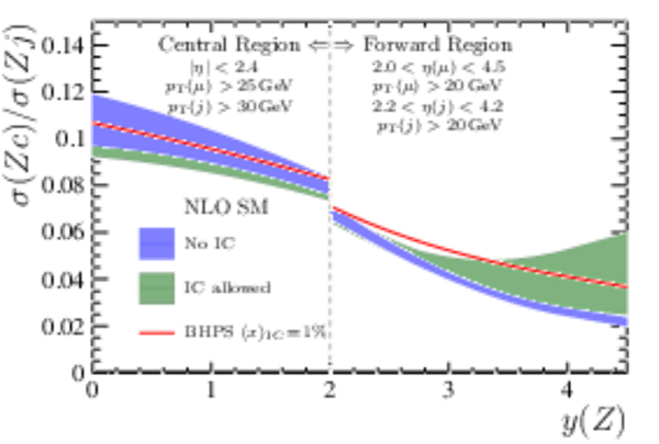
NLO SM predictions [29] for $\mathcal{R}^c{\raisebox{-0.2em}{\scriptstyle j}}$ without IC [42], allowing for potential IC [39], and with the valence-like IC predicted by BHPS with a mean momentum fraction of 1% [38]. The fiducial region from Ref. [41] is used for $ y( Z ) < 2$; otherwise the fiducial region of this analysis is employed. The broadening of the error band that arises in the forward region, when allowing for IC, is due to the lack of sensitivity to valence-like IC from previous experiments. More details on these calculations are provided in the Supplemental Material [43]. The error bands shown for the first two predictions display the 68% confidence-level regions. Only the central value is shown for BHPS due to the charm PDF being fixed.

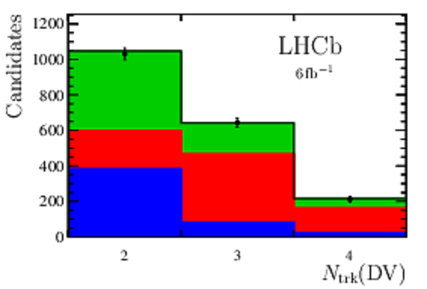
Distributions of (left) $m_{\rm cor}({\rm DV})$ and (right) $N_{\rm trk}({\rm DV})$ for all DV-tagged candidates in the $ Z j$ data sample reconstructed in the fiducial region with the projections of the fit results superimposed.

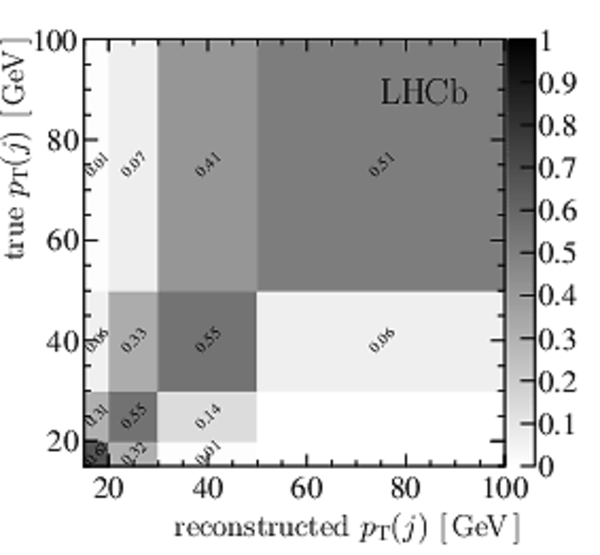
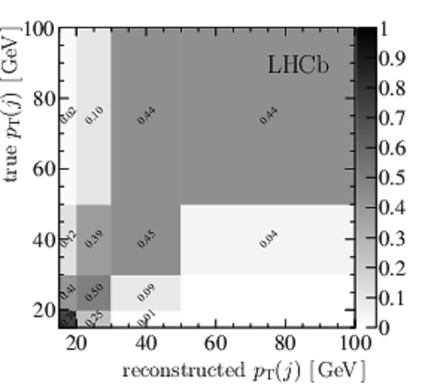
The detector-response matrix for $c$-tagged jets. The shading represents the interval-to-interval migration probabilities ranging from (white) 0 to (black) 1. Numerical labels are only shown for values greater than 1%. Jets with true (reconstructed) $ p_{\mathrm{T}} (j)$ in the 20--100 $\text{ Ge V}$ region but for which the reconstructed (true) $ p_{\mathrm{T}} (j)$ is either below 15 $\text{ Ge V}$ or above 100 $\text{ Ge V}$ are included in the unfolding but not shown graphically.

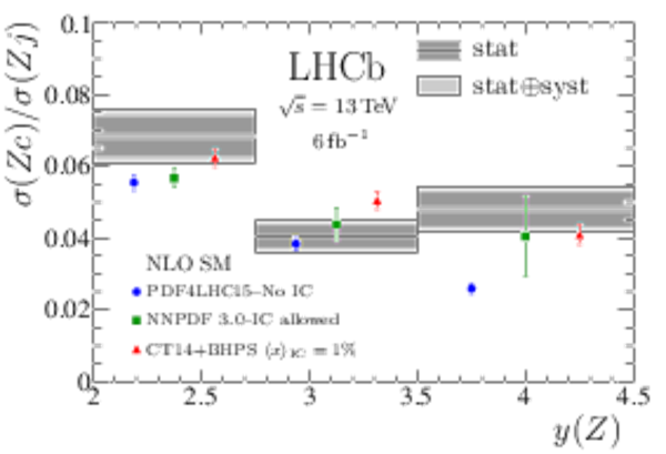
Measured $\mathcal{R}^c{\raisebox{-0.2em}{\scriptstyle j}}$ distribution (gray bands) for three intervals of forward $ Z $ rapidity, compared to NLO SM predictions [29] without IC [42], with the charm PDF shape allowed to vary (hence, permitting IC) [39,78], and with IC as predicted by BHPS with a mean momentum fraction of 1% [38]. The predictions are offset in each interval to improve visibility.

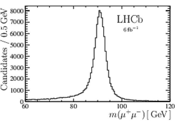
Dimuon invariant mass distribution for the $ Z j$ sample.

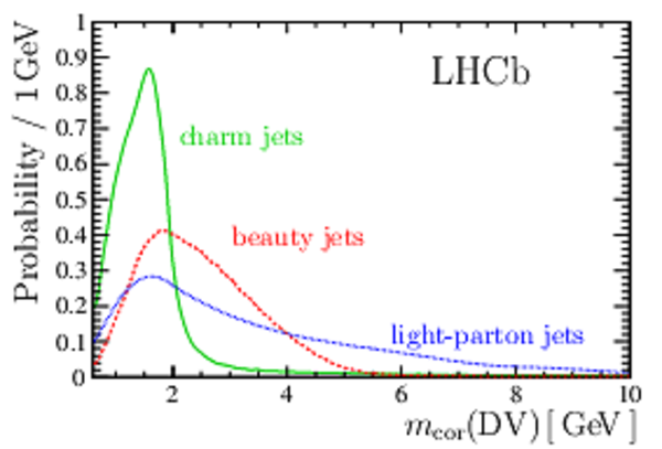
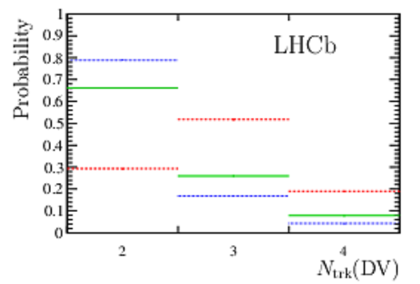
Probability density functions for the DV features used in the $c$-tagging fits for $c$, $b$, and light-parton jets: (left) the corrected mass and (right) the track multiplicity.

The detector-response matrix for inclusive $ Z j$ events. The shading represents the interval-to-interval migration probabilities ranging from (white) 0 to (black) 1. Numerical labels are only shown for values greater than 1%. Jets with true (reconstructed) $ p_{\mathrm{T}} (j)$ in the 20--100 $\text{ Ge V}$ region but for which the reconstructed (true) $ p_{\mathrm{T}} (j)$ is either below 15 $\text{ Ge V}$ or above 100 $\text{ Ge V}$ are included in the unfolding but not shown graphically.

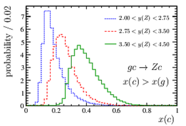
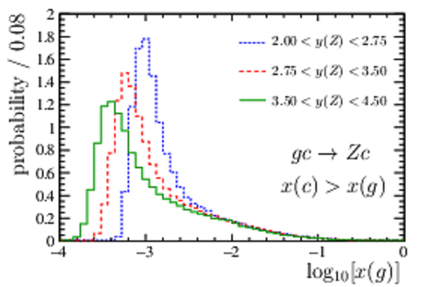
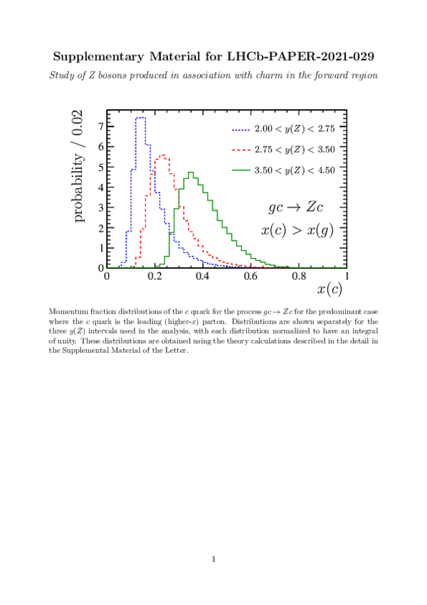
Momentum fraction distributions of the (left) $c$ quark and (right) gluon for the process $g c \rightarrow Z c$ in the predominant scenario where the $c$ quark is the leading (higher-$x$) parton. Distributions are shown separately for the three $y(Z)$ intervals used in the analysis, with each distribution normalized to have an integral of unity. These distributions are obtained using the theory calculations described in detail here in the Supplemental Material.

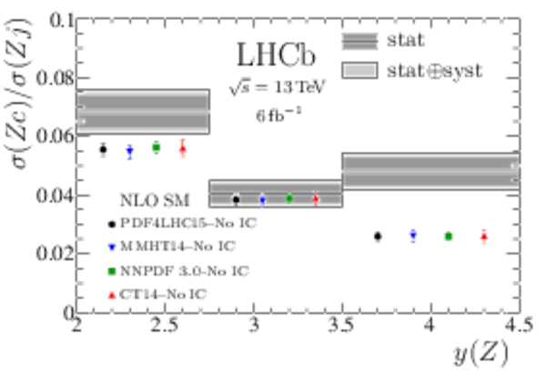
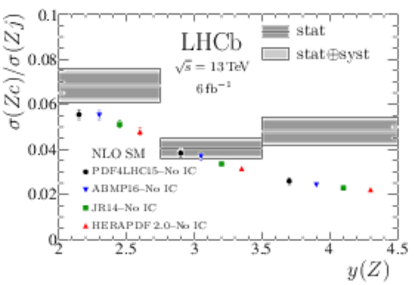
Measured $\mathcal{R}^c{\raisebox{-0.2em}{\scriptstyle j}}$ distribution (gray bands) for three intervals of forward $ Z $ rapidity, compared to NLO SM predictions [29] using various PDF sets. The predictions are offset in each interval to improve visibility. The left plot shows that the three PDF sets [78,79,81] on which the PDF4LHC15 [42] set is formed from all provide consistent predictions for $\mathcal{R}^c{\raisebox{-0.2em}{\scriptstyle j}}$ . The right plot shows that the ABM16 [82], JR14 [83], and HERAPDF 2.0 [84] PDF sets also provide qualitatively similar predictions, though the JR14 and HERAPDF 2.0 predictions are shifted to lower $\mathcal{R}^c{\raisebox{-0.2em}{\scriptstyle j}}$ values.

Animated gif made out of all figures.

Definition of the fiducial region.

Relative systematic uncertainties on $\mathcal{R}^c{\raisebox{-0.2em}{\scriptstyle j}}$ , where ranges indicate that the value depends on the $ y( Z )$ intervals.

Numerical results for the $\mathcal{R}^c{\raisebox{-0.2em}{\scriptstyle j}}$ measurements, where the first uncertainty is statistical and the second is systematic.

Numerical results for the ratios $r^c_{j}(i/k) \equiv \mathcal{R}^c{\raisebox{-0.2em}{\scriptstyle j}} [ y( Z ) _i] / \mathcal{R}^c{\raisebox{-0.2em}{\scriptstyle j}} [ y( Z ) _k]$, where the first uncertainty is statistical and the second is systematic for each result. The labels low, mid, and high refer to $ y( Z )$ ranges of 2.00--2.75, 2.75--3.50 and 3.50--4.50, respectively.

Supplementary material full pdf