Search for the lepton-flavour violating decays $B^0 \to K^{*0} \mu^\pm e^\mp$ and $B_s^0 \to \phi \mu^\pm e^\mp$
[to restricted-access page]Information
LHCb-PAPER-2022-008
CERN-EP-2022-097
arXiv:2207.04005 [PDF]
(Submitted on 08 Jul 2022)
JHEP 06 (2023) 073
Inspire 2107941
Tools
Abstract
A search for the lepton-flavour violating decays $B^0 \to K^{*0} \mu^\pm e^\mp$ and $B_s^0 \to \phi \mu^\pm e^\mp$ is presented, using proton-proton collision data collected by the LHCb detector at the LHC, corresponding to an integrated luminosity of $9 \text{fb}^{-1}$. No significant signals are observed and upper limits of \begin{align} {\cal B}( B^0 \to K^{*0} \mu^+ e^- ) &< \phantom{1}5.7\times 10^{-9} (6.9\times 10^{-9}),\newline {\cal B}( B^0 \to K^{*0} \mu^- e^+ ) &< \phantom{1}6.8\times 10^{-9} (7.9\times 10^{-9}),\newline {\cal B}( B^0 \to K^{*0} \mu^\pm e^\mp ) &< 10.1\times 10^{-9} (11.7\times 10^{-9}),\newline {\cal B}( B_s^0 \to \phi \mu^\pm e^\mp ) &< 16.0\times 10^{-9} (19.8\times 10^{-9}) \end{align} are set at $90\% (95\%)$ confidence level. These results constitute the world's most stringent limits to date, with the limit on the decay $B_s^0 \to \phi \mu^\pm e^\mp$ the first being set. In addition, limits are reported for scalar and left-handed lepton-flavour violating New Physics scenarios.
Figures and captions
|
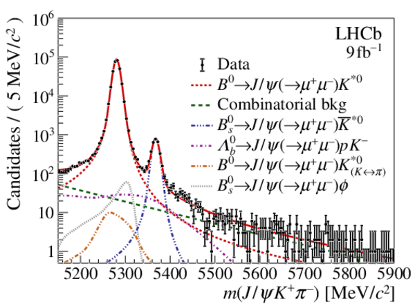
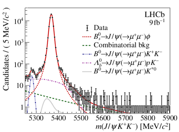
Mass distributions for the normalisation channels (left) $ B ^0 \rightarrow { J \mskip -3mu/\mskip -2mu\psi } (\rightarrow \mu ^+\mu ^- ) K ^{*0} $ and (right) $ B ^0_ s \rightarrow { J \mskip -3mu/\mskip -2mu\psi } (\rightarrow \mu ^+\mu ^- )\phi $ combining the different data taking periods, overlaid with the fit results. |
Fig1a.pdf [28 KiB] HiDef png [548 KiB] Thumbnail [377 KiB] *.C file |
|
|
Fig1b.pdf [24 KiB] HiDef png [462 KiB] Thumbnail [327 KiB] *.C file |
|
|
|
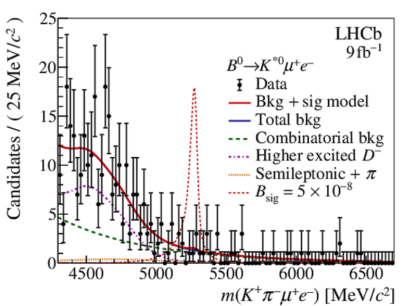
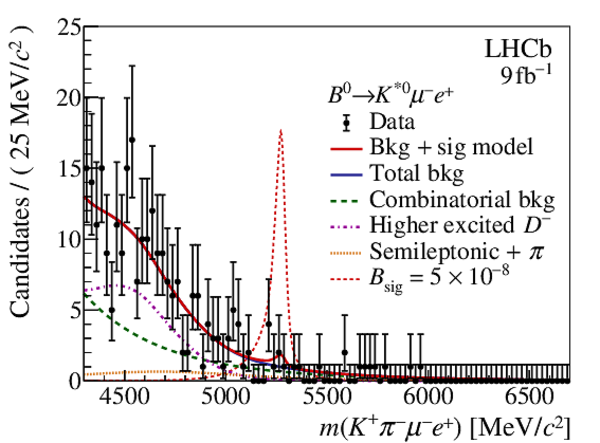
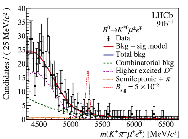
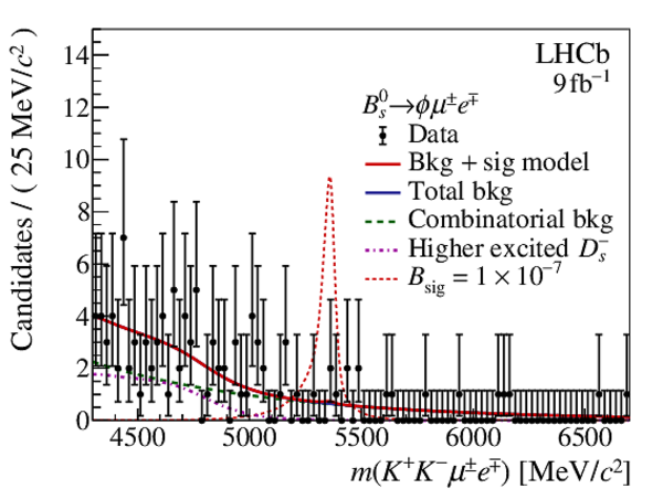
Mass distributions for (top left) $ B ^0 \rightarrow K ^{*0} \mu^+ e^- $, (top right) $ B ^0 \rightarrow K ^{*0} \mu^- e^+ $, (bottom left) $ B ^0 \rightarrow K ^{*0} \mu^\pm e^\mp $, and (bottom right) $ B ^0_ s \rightarrow \phi\mu^\pm e^\mp $ candidates. The data are overlaid with the fit results. For illustration, the signal shape, scaled to a branching fraction of $5\times 10^{-8}$ for the $ B ^0 \rightarrow K ^{*0} \mu^\pm e^\mp $ decays and $1\times 10^{-7}$ for $ B ^0_ s \rightarrow \phi\mu^\pm e^\mp $, is drawn as red dashed line. |
Fig2a.pdf [23 KiB] HiDef png [358 KiB] Thumbnail [299 KiB] *.C file |
|
|
Fig2b.pdf [23 KiB] HiDef png [345 KiB] Thumbnail [291 KiB] *.C file |
|
|
|
Fig2c.pdf [23 KiB] HiDef png [361 KiB] Thumbnail [308 KiB] *.C file |
|
|
|
Fig2d.pdf [22 KiB] HiDef png [321 KiB] Thumbnail [280 KiB] *.C file |
|
|
|
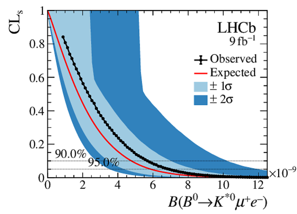
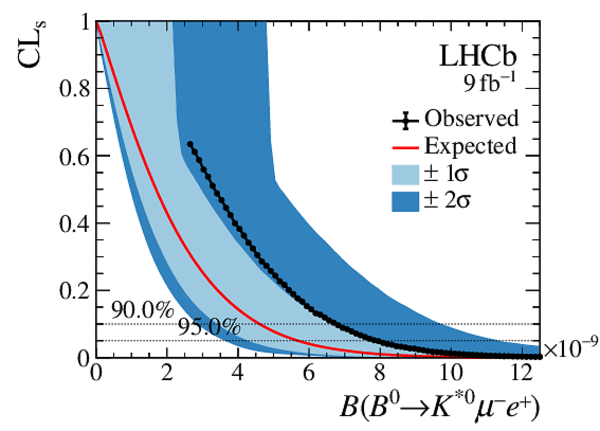
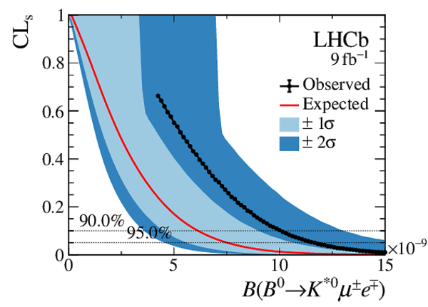
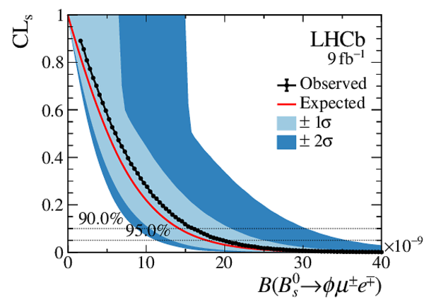
Observed and expected (background-only hypothesis) limits for (top left) $ B ^0 \rightarrow K ^{*0} \mu^+ e^- $, (top right) $ B ^0 \rightarrow K ^{*0} \mu^- e^+ $, (bottom left) $ B ^0 \rightarrow K ^{*0} \mu^\pm e^\mp $, and (bottom right) $ B ^0_ s \rightarrow \phi\mu^\pm e^\mp $. |
Fig3a.pdf [20 KiB] HiDef png [362 KiB] Thumbnail [247 KiB] *.C file |
|
|
Fig3b.pdf [20 KiB] HiDef png [346 KiB] Thumbnail [236 KiB] *.C file |
|
|
|
Fig3c.pdf [19 KiB] HiDef png [349 KiB] Thumbnail [235 KiB] *.C file |
|
|
|
Fig3d.pdf [20 KiB] HiDef png [351 KiB] Thumbnail [233 KiB] *.C file |
|
|
|
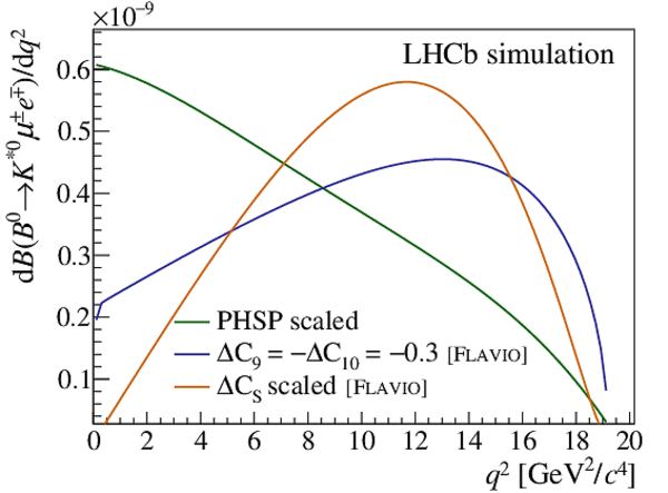
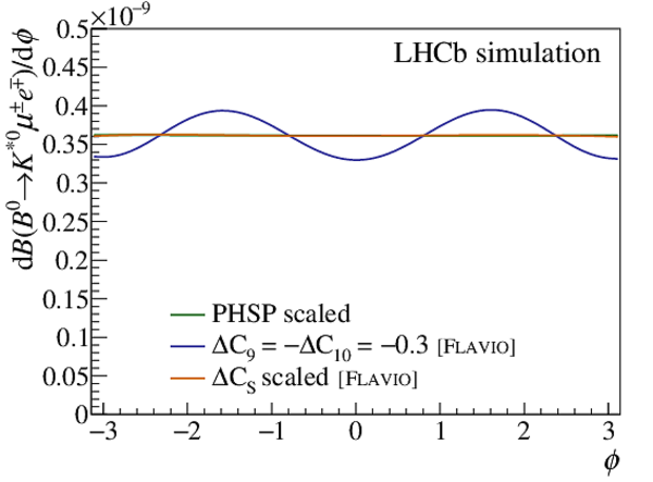
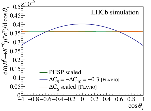
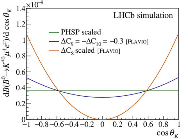
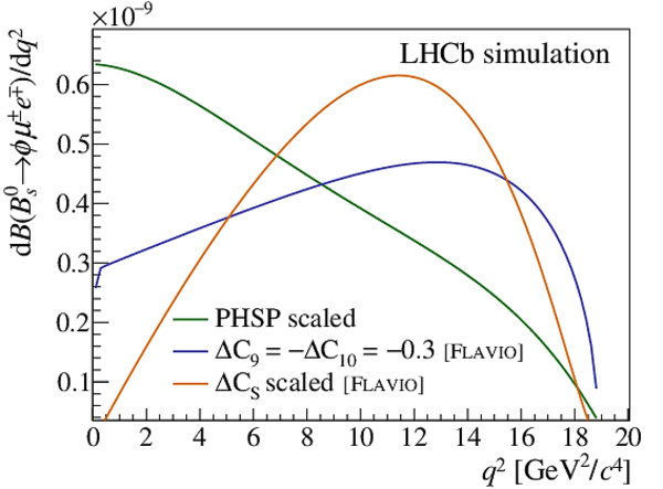
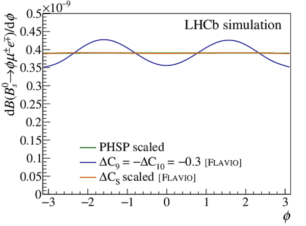
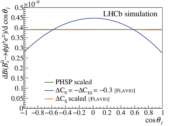
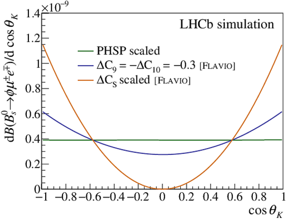
Differential decay rate as a function of the four-momentum transfer $ q^2$ and the three decay angles in a left-handed ($C_9^{\mu e}=-C_{10}^{\mu e}\neq 0$) NP model for (top) the signal decay $ B ^0 \rightarrow K ^{*0} \mu^\pm e^\mp $ and (bottom) $ B ^0_ s \rightarrow \phi\mu^\pm e^\mp $. The left-handed NP scenario is compared with the nominal phase space and a scalar ($C_S^{\mu e}\neq 0$) model, normalised to the same area. |
Fig4a.pdf [15 KiB] HiDef png [290 KiB] Thumbnail [206 KiB] *.C file |
|
|
Fig4b.pdf [15 KiB] HiDef png [191 KiB] Thumbnail [157 KiB] *.C file |
|
|
|
Fig4c.pdf [15 KiB] HiDef png [216 KiB] Thumbnail [182 KiB] *.C file |
|
|
|
Fig4d.pdf [15 KiB] HiDef png [244 KiB] Thumbnail [185 KiB] *.C file |
|
|
|
Fig4e.pdf [15 KiB] HiDef png [288 KiB] Thumbnail [203 KiB] *.C file |
|
|
|
Fig4f.pdf [15 KiB] HiDef png [192 KiB] Thumbnail [157 KiB] *.C file |
|
|
|
Fig4g.pdf [15 KiB] HiDef png [217 KiB] Thumbnail [182 KiB] *.C file |
|
|
|
Fig4h.pdf [15 KiB] HiDef png [250 KiB] Thumbnail [187 KiB] *.C file |
|
|
|
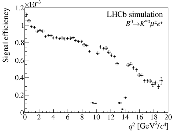
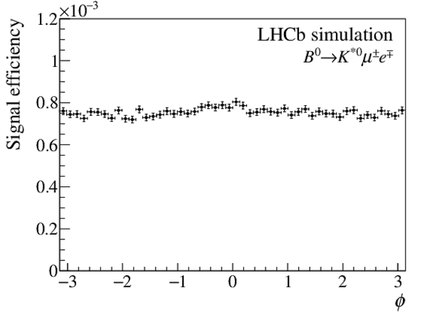
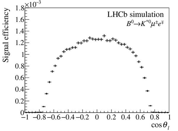
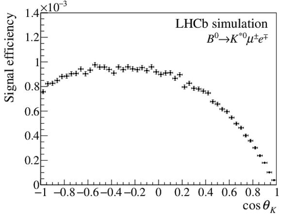
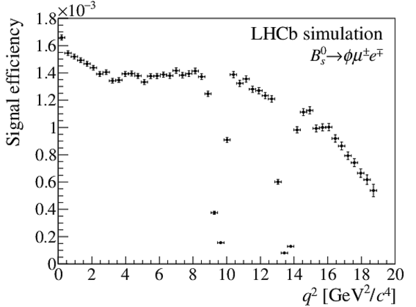
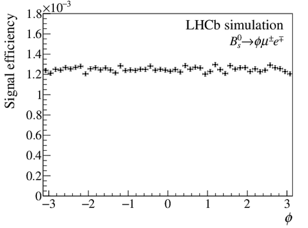
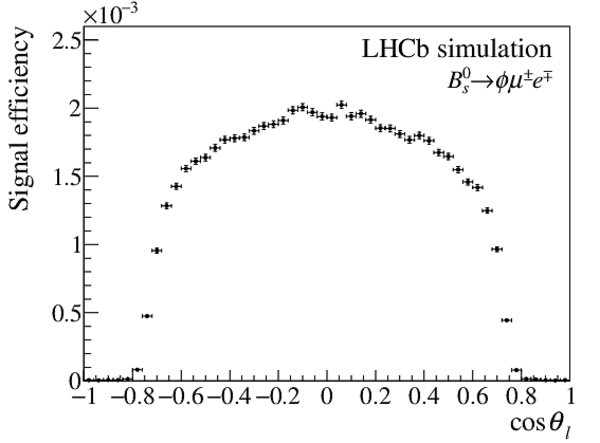
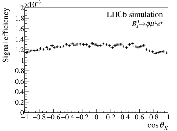
Reconstruction and selection efficiency, combined for the 2011 - 2018 samples, for (top) $ B ^0 \rightarrow K ^{*0} \mu^\pm e^\mp $ and (bottom) $ B ^0_ s \rightarrow \phi\mu^\pm e^\mp $ signal decays depending on $ q^2$ and the three decay angles $\cos{\theta_\ell} $, $\cos{\theta_K} $, and $\phi$. The selection efficiency drops in the $ q^2$ region around the $ { J \mskip -3mu/\mskip -2mu\psi } $ and $\psi {(2S)} $ masses as a result of the veto against misidentified backgrounds. |
Fig5a.pdf [18 KiB] HiDef png [114 KiB] Thumbnail [59 KiB] *.C file |
|
|
Fig5b.pdf [18 KiB] HiDef png [101 KiB] Thumbnail [52 KiB] *.C file |
|
|
|
Fig5c.pdf [18 KiB] HiDef png [116 KiB] Thumbnail [60 KiB] *.C file |
|
|
|
Fig5d.pdf [18 KiB] HiDef png [119 KiB] Thumbnail [61 KiB] *.C file |
|
|
|
Fig5e.pdf [18 KiB] HiDef png [119 KiB] Thumbnail [62 KiB] *.C file |
|
|
|
Fig5f.pdf [18 KiB] HiDef png [104 KiB] Thumbnail [55 KiB] *.C file |
|
|
|
Fig5g.pdf [18 KiB] HiDef png [107 KiB] Thumbnail [54 KiB] *.C file |
|
|
|
Fig5h.pdf [18 KiB] HiDef png [122 KiB] Thumbnail [63 KiB] *.C file |
|
|
|
Animated gif made out of all figures. |
PAPER-2022-008.gif Thumbnail |

|
![HiDef png [548 KiB]](Directory_LHCb-PAPER-2022-008/hidef_Fig1a.png)
![HiDef png [462 KiB]](Directory_LHCb-PAPER-2022-008/hidef_Fig1b.png)
![HiDef png [358 KiB]](Directory_LHCb-PAPER-2022-008/hidef_Fig2a.png)
![HiDef png [345 KiB]](Directory_LHCb-PAPER-2022-008/hidef_Fig2b.png)
![HiDef png [361 KiB]](Directory_LHCb-PAPER-2022-008/hidef_Fig2c.png)
![HiDef png [321 KiB]](Directory_LHCb-PAPER-2022-008/hidef_Fig2d.png)
![HiDef png [362 KiB]](Directory_LHCb-PAPER-2022-008/hidef_Fig3a.png)
![HiDef png [346 KiB]](Directory_LHCb-PAPER-2022-008/hidef_Fig3b.png)
![HiDef png [349 KiB]](Directory_LHCb-PAPER-2022-008/hidef_Fig3c.png)
![HiDef png [351 KiB]](Directory_LHCb-PAPER-2022-008/hidef_Fig3d.png)
![HiDef png [290 KiB]](Directory_LHCb-PAPER-2022-008/hidef_Fig4a.png)
![HiDef png [191 KiB]](Directory_LHCb-PAPER-2022-008/hidef_Fig4b.png)
![HiDef png [216 KiB]](Directory_LHCb-PAPER-2022-008/hidef_Fig4c.png)
![HiDef png [244 KiB]](Directory_LHCb-PAPER-2022-008/hidef_Fig4d.png)
![HiDef png [288 KiB]](Directory_LHCb-PAPER-2022-008/hidef_Fig4e.png)
![HiDef png [192 KiB]](Directory_LHCb-PAPER-2022-008/hidef_Fig4f.png)
![HiDef png [217 KiB]](Directory_LHCb-PAPER-2022-008/hidef_Fig4g.png)
![HiDef png [250 KiB]](Directory_LHCb-PAPER-2022-008/hidef_Fig4h.png)
![HiDef png [114 KiB]](Directory_LHCb-PAPER-2022-008/hidef_Fig5a.png)
![HiDef png [101 KiB]](Directory_LHCb-PAPER-2022-008/hidef_Fig5b.png)
![HiDef png [116 KiB]](Directory_LHCb-PAPER-2022-008/hidef_Fig5c.png)
![HiDef png [119 KiB]](Directory_LHCb-PAPER-2022-008/hidef_Fig5d.png)
![HiDef png [119 KiB]](Directory_LHCb-PAPER-2022-008/hidef_Fig5e.png)
![HiDef png [104 KiB]](Directory_LHCb-PAPER-2022-008/hidef_Fig5f.png)
![HiDef png [107 KiB]](Directory_LHCb-PAPER-2022-008/hidef_Fig5g.png)
![HiDef png [122 KiB]](Directory_LHCb-PAPER-2022-008/hidef_Fig5h.png)
Tables and captions
|
Normalisation mode yields $[10^3]$ for different periods of data taking. |
Table_1.pdf [67 KiB] HiDef png [39 KiB] Thumbnail [19 KiB] tex code |

|
|
Normalisation constant $\alpha$ $[10^{-9}]$ with associated statistical and systematic uncertainties, added in quadrature, for different periods of data taking. The total uncertainty is dominated by systematic effects, which are discussed in Sec. 6. The year-to-year $B^0/B_s^0$ ratio variation is due to different BDT criteria against combinatorial background, tuned individually for each data taking period and mode. |
Table_2.pdf [68 KiB] HiDef png [72 KiB] Thumbnail [37 KiB] tex code |

|
|
Sources of relative systematic uncertainties $[\%]$ on the normalisation constant $\alpha$ defined in Eq. 1. Where the uncertainty depends on the year of data taking, a range is provided. |
Table_3.pdf [80 KiB] HiDef png [91 KiB] Thumbnail [42 KiB] tex code |

|
|
Expected (background-only hypothesis) and observed limits $[10^{-9}]$ at $90\%$ ($95\%$) CL. |
Table_4.pdf [68 KiB] HiDef png [77 KiB] Thumbnail [35 KiB] tex code |

|
|
Exclusion limits $[10^{-9}]$ on the $B_{(s)}^0$ branching fractions for a scalar ($C_s^{\mu e}\neq 0$) and left-handed ($C_9^{\mu e}=-C_{10}^{\mu e}\neq 0$) NP model at $90\%$ ($95\%$) CL. |
Table_5.pdf [68 KiB] HiDef png [76 KiB] Thumbnail [35 KiB] tex code |

|
![HiDef png [39 KiB]](Directory_LHCb-PAPER-2022-008/hidef_Table_1.png)
![HiDef png [72 KiB]](Directory_LHCb-PAPER-2022-008/hidef_Table_2.png)
![HiDef png [91 KiB]](Directory_LHCb-PAPER-2022-008/hidef_Table_3.png)
![HiDef png [77 KiB]](Directory_LHCb-PAPER-2022-008/hidef_Table_4.png)
![HiDef png [76 KiB]](Directory_LHCb-PAPER-2022-008/hidef_Table_5.png)
Created on 20 April 2024.