Search for the baryon- and lepton-number violating decays $B^0\to p\mu^-$ and $B^0_s\to p\mu^-$
[to restricted-access page]Information
LHCb-PAPER-2022-022
CERN-EP-2022-195
arXiv:2210.10412 [PDF]
(Submitted on 19 Oct 2022)
Phys. Rev. D108 (2023) 012021
Inspire 2683002
Tools
Abstract
A search for the baryon- and lepton-number violating decays $B^0\to p\mu^-$ and $B^0_s\to p\mu^-$ is performed at the LHCb experiment using data collected in proton-proton collisions at $\sqrt{s}$ = 7, 8 and 13 TeV, corresponding to integrated luminosities of 1, 2 and 6 fb$^{-1}$, respectively. No significant signal for $B^0\to p\mu^-$ and $B^0_s\to p\mu^-$ decays is found and the upper limits on the branching fractions are determined to be ${\cal B}(B^0\to p\mu^-)<2.6 (3.1)\times10^{-9}$ and ${\cal B}(B^0_s\to p\mu^-)<12.1 (14.0)\times10^{-9}$, respectively, at 90$\%$ (95$\%$) confidence level. These are the first limits on these decays to date.
Figures and captions
|
Hypothetical Feynman diagrams of $ B ^0_{( s )} \rightarrow p \ell^{-}$ and $\overline p \ell^{+}$ mediated by a hypothetical $Y$ boson. |
Fig1a.pdf [25 KiB] HiDef png [19 KiB] Thumbnail [10 KiB] *.C file |

|
|
Fig1b.pdf [34 KiB] HiDef png [23 KiB] Thumbnail [12 KiB] *.C file |

|
|
|
Fig1c.pdf [27 KiB] HiDef png [26 KiB] Thumbnail [13 KiB] *.C file |

|
|
|
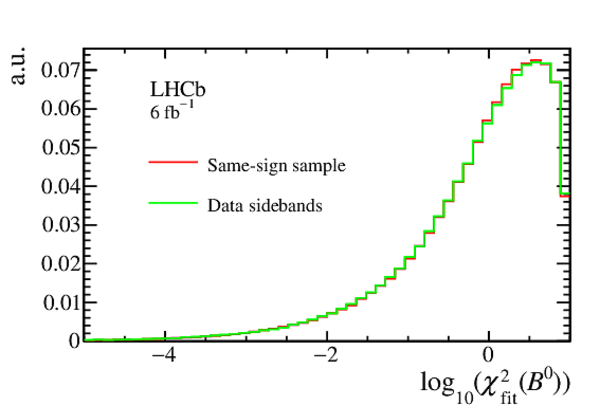
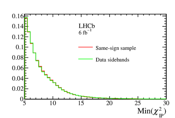
Comparison of the distributions of the $ B ^0$ vertex fit $\chi^2$ ($\chi^2_{\mathrm{fit}}(B^0)$) and the minimum $\chi^2_{\text{IP}}$ of the two tracks in the final state ($\mathrm{Min}(\chi^2_{\mathrm{IP}})$), for the same-sign sample and data sidebands in Run 2. |
Fig2a.eps [12 KiB] HiDef png [118 KiB] Thumbnail [116 KiB] *.C file |
|
|
Fig2b.eps [12 KiB] HiDef png [119 KiB] Thumbnail [115 KiB] *.C file |
|
|
|
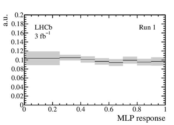
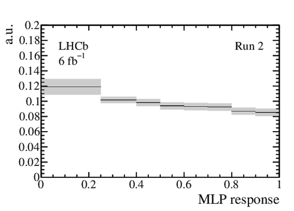
Expected distribution of the MLP response for $ B ^0_{( s )} \rightarrow p \mu ^- $ decays as obtained from the $ B ^0 \rightarrow K ^+ \pi ^- $ control channel, for (left) Run 1 and (right) Run 2 data. The total (statistical and systematic combined) uncertainty is shown as a light grey band, and the thickness of each horizontal line at the centre indicates the statistical uncertainty. Each interval is normalised to its width. |
Fig3a.eps [13 KiB] HiDef png [83 KiB] Thumbnail [49 KiB] *.C file |
|
|
Fig3b.eps [13 KiB] HiDef png [82 KiB] Thumbnail [48 KiB] *.C file |
|
|
|
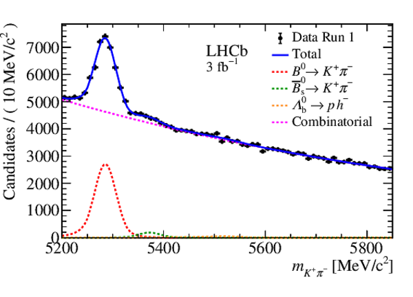
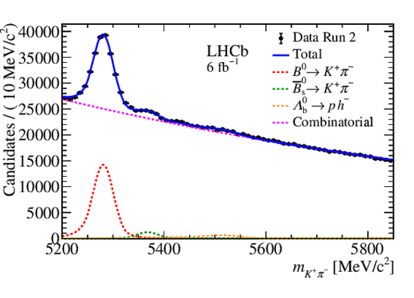
Mass distribution of $ B ^0 \rightarrow K ^+ \pi ^- $ candidates in data for (left) Run 1 and (right) Run 2. The results of the invariant mass fits are superimposed. |
Fig4a.eps [29 KiB] HiDef png [262 KiB] Thumbnail [208 KiB] *.C file |
|
|
Fig4b.eps [33 KiB] HiDef png [274 KiB] Thumbnail [220 KiB] *.C file |
|
|
|
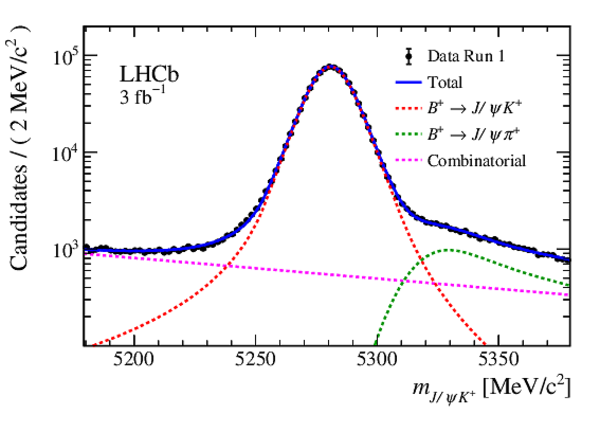
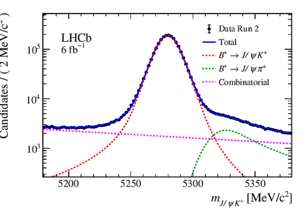
Mass distribution of $ B ^+ \rightarrow { J \mskip -3mu/\mskip -2mu\psi } K ^+ $ candidates in data for (left) Run 1 and (right) Run 2. The results of the invariant mass fits are superimposed. |
Fig5a.eps [33 KiB] HiDef png [220 KiB] Thumbnail [175 KiB] *.C file |
|
|
Fig5b.eps [33 KiB] HiDef png [218 KiB] Thumbnail [174 KiB] *.C file |
|
|
|
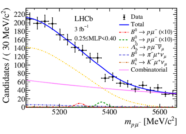
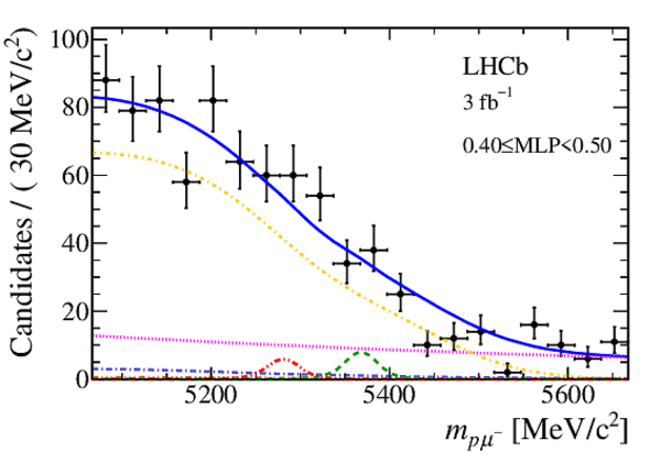
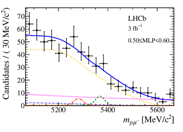
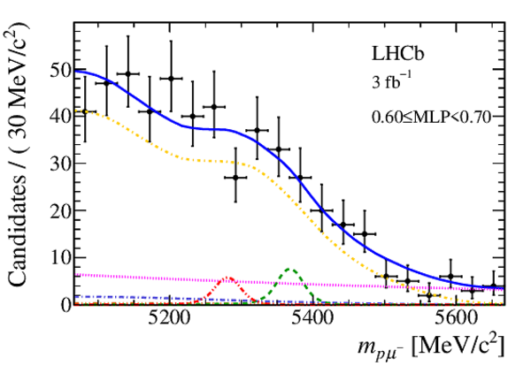
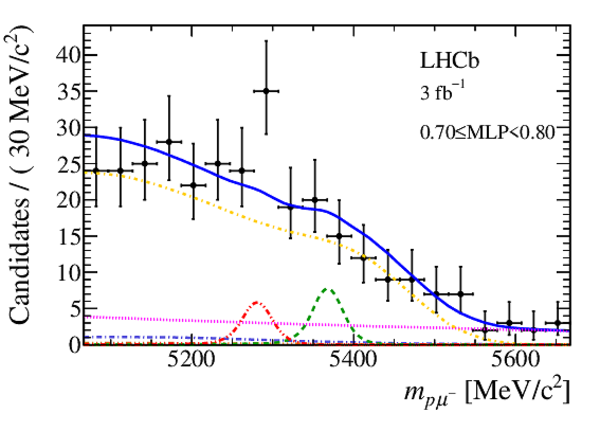
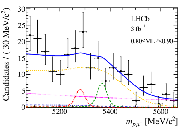
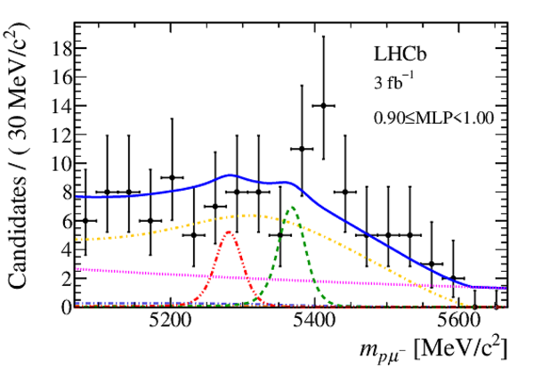
Mass distribution of signal candidates (black dots) for Run 1 samples in regions of MLP. The results of the fit described in the text are also shown. The contributions from the two signal channels, $ B ^0 \rightarrow p \mu ^- $ (red dashed lines) and $ B ^0_ s \rightarrow p \mu ^- $ (green dashed lines), are scaled by a factor of 10 for better visibility. |
Fig6a.eps [26 KiB] HiDef png [322 KiB] Thumbnail [270 KiB] *.C file |
|
|
Fig6b.eps [17 KiB] HiDef png [247 KiB] Thumbnail [189 KiB] *.C file |
|
|
|
Fig6c.eps [18 KiB] HiDef png [253 KiB] Thumbnail [200 KiB] *.C file |
|
|
|
Fig6d.eps [18 KiB] HiDef png [252 KiB] Thumbnail [194 KiB] *.C file |
|
|
|
Fig6e.eps [19 KiB] HiDef png [257 KiB] Thumbnail [202 KiB] *.C file |
|
|
|
Fig6f.eps [18 KiB] HiDef png [255 KiB] Thumbnail [197 KiB] *.C file |
|
|
|
Fig6g.eps [19 KiB] HiDef png [255 KiB] Thumbnail [200 KiB] *.C file |
|
|
|
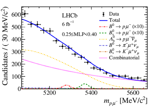
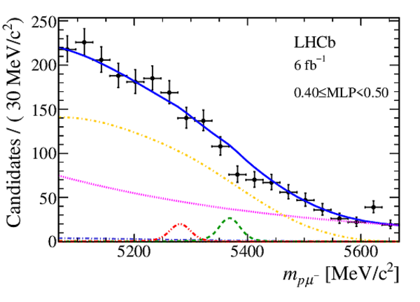
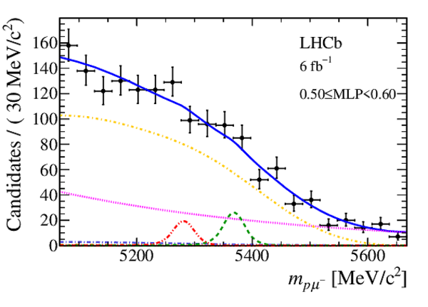
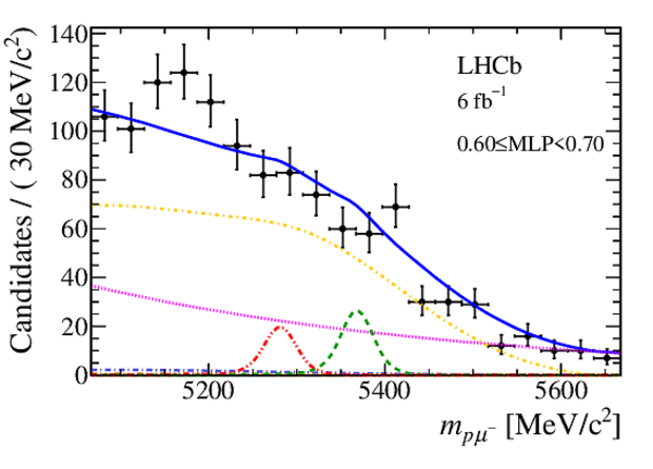
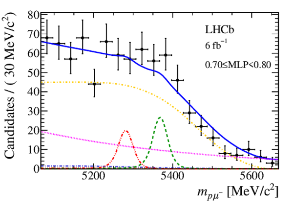
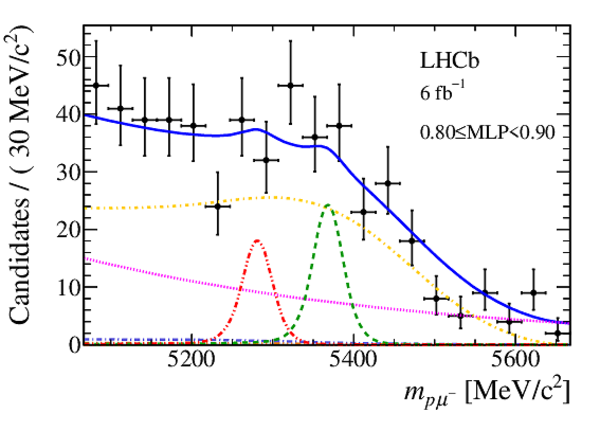
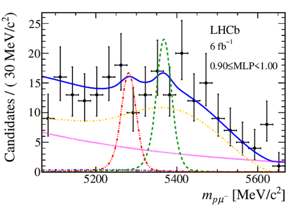
Mass distribution of signal candidates (black dots) for Run 2 samples in regions of MLP. The results of the fit described in the text are also shown. The contributions from the two signal channels, $ B ^0 \rightarrow p \mu ^- $ (red dashed lines) and $ B ^0_ s \rightarrow p \mu ^- $ (green dashed lines), are scaled by a factor of 10 for better visibility. |
Fig7a.eps [24 KiB] HiDef png [303 KiB] Thumbnail [247 KiB] *.C file |
|
|
Fig7b.eps [17 KiB] HiDef png [247 KiB] Thumbnail [187 KiB] *.C file |
|
|
|
Fig7c.eps [18 KiB] HiDef png [254 KiB] Thumbnail [201 KiB] *.C file |
|
|
|
Fig7d.eps [18 KiB] HiDef png [252 KiB] Thumbnail [196 KiB] *.C file |
|
|
|
Fig7e.eps [19 KiB] HiDef png [268 KiB] Thumbnail [208 KiB] *.C file |
|
|
|
Fig7f.eps [17 KiB] HiDef png [260 KiB] Thumbnail [200 KiB] *.C file |
|
|
|
Fig7g.eps [18 KiB] HiDef png [281 KiB] Thumbnail [208 KiB] *.C file |
|
|
|
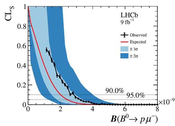
Results from the CLs scan used to obtain the limit on (left) $\mathcal{B} ( B ^0 \rightarrow p \mu ^- )$ and (right) $\mathcal{B} ( B ^0_ s \rightarrow p \mu ^- )$. The background-only expectation is shown by the red line and the 1$\sigma$ and 2$\sigma$ bands are shown as light blue and blue bands respectively. The observation is shown as the solid black line. The two dashed lines intersecting with the observation indicate the limits at 90% and 95% CL for the upper and lower line, respectively. |
Fig8a.eps [16 KiB] HiDef png [298 KiB] Thumbnail [203 KiB] *.C file |
|
|
Fig8b.eps [16 KiB] HiDef png [295 KiB] Thumbnail [205 KiB] *.C file |

|
|
|
Animated gif made out of all figures. |
PAPER-2022-022.gif Thumbnail |

|
![HiDef png [19 KiB]](Directory_LHCb-PAPER-2022-022/hidef_Fig1a.png)
![HiDef png [23 KiB]](Directory_LHCb-PAPER-2022-022/hidef_Fig1b.png)
![HiDef png [26 KiB]](Directory_LHCb-PAPER-2022-022/hidef_Fig1c.png)
![HiDef png [118 KiB]](Directory_LHCb-PAPER-2022-022/hidef_Fig2a.png)
![HiDef png [119 KiB]](Directory_LHCb-PAPER-2022-022/hidef_Fig2b.png)
![HiDef png [83 KiB]](Directory_LHCb-PAPER-2022-022/hidef_Fig3a.png)
![HiDef png [82 KiB]](Directory_LHCb-PAPER-2022-022/hidef_Fig3b.png)
![HiDef png [262 KiB]](Directory_LHCb-PAPER-2022-022/hidef_Fig4a.png)
![HiDef png [274 KiB]](Directory_LHCb-PAPER-2022-022/hidef_Fig4b.png)
![HiDef png [220 KiB]](Directory_LHCb-PAPER-2022-022/hidef_Fig5a.png)
![HiDef png [218 KiB]](Directory_LHCb-PAPER-2022-022/hidef_Fig5b.png)
![HiDef png [322 KiB]](Directory_LHCb-PAPER-2022-022/hidef_Fig6a.png)
![HiDef png [247 KiB]](Directory_LHCb-PAPER-2022-022/hidef_Fig6b.png)
![HiDef png [253 KiB]](Directory_LHCb-PAPER-2022-022/hidef_Fig6c.png)
![HiDef png [252 KiB]](Directory_LHCb-PAPER-2022-022/hidef_Fig6d.png)
![HiDef png [257 KiB]](Directory_LHCb-PAPER-2022-022/hidef_Fig6e.png)
![HiDef png [255 KiB]](Directory_LHCb-PAPER-2022-022/hidef_Fig6f.png)
![HiDef png [255 KiB]](Directory_LHCb-PAPER-2022-022/hidef_Fig6g.png)
![HiDef png [303 KiB]](Directory_LHCb-PAPER-2022-022/hidef_Fig7a.png)
![HiDef png [247 KiB]](Directory_LHCb-PAPER-2022-022/hidef_Fig7b.png)
![HiDef png [254 KiB]](Directory_LHCb-PAPER-2022-022/hidef_Fig7c.png)
![HiDef png [252 KiB]](Directory_LHCb-PAPER-2022-022/hidef_Fig7d.png)
![HiDef png [268 KiB]](Directory_LHCb-PAPER-2022-022/hidef_Fig7e.png)
![HiDef png [260 KiB]](Directory_LHCb-PAPER-2022-022/hidef_Fig7f.png)
![HiDef png [281 KiB]](Directory_LHCb-PAPER-2022-022/hidef_Fig7g.png)
![HiDef png [298 KiB]](Directory_LHCb-PAPER-2022-022/hidef_Fig8a.png)
![HiDef png [295 KiB]](Directory_LHCb-PAPER-2022-022/hidef_Fig8b.png)
Tables and captions
|
Expected and observed upper limits for $\mathcal{B} ( B ^0 \rightarrow p \mu ^- )$ and $\mathcal{B} ( B ^0_ s \rightarrow p \mu ^- )$ at 90% (95%) CL, with systematic effects included. No signal is assumed for the expected upper limits. |
Table_1.pdf [68 KiB] HiDef png [39 KiB] Thumbnail [19 KiB] tex code |

|
![HiDef png [39 KiB]](Directory_LHCb-PAPER-2022-022/hidef_Table_1.png)
Created on 20 April 2024.