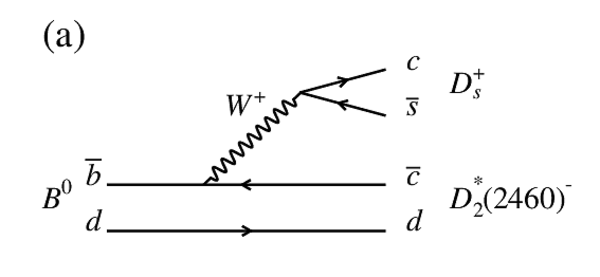
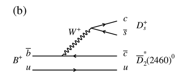
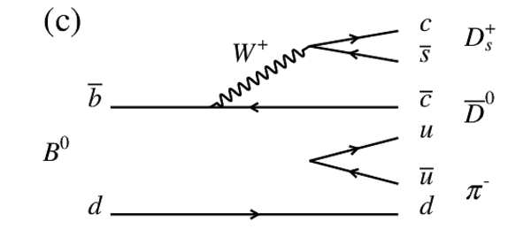
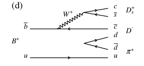
Feynman diagrams for the dominant tree-level amplitudes contributing to (a) $ B ^0 \rightarrow \overline{ D } {}^0 D ^+_ s \pi ^- $ and (b) $ B ^+ \rightarrow D ^- D ^+_ s \pi ^+ $ decays with intermediate $D\pi$ resonances; and nonresonant three body decays of (c) $ B ^0 \rightarrow \overline{ D } {}^0 D ^+_ s \pi ^- $ and (d) $ B ^+ \rightarrow D ^- D ^+_ s \pi ^+ $ decays.

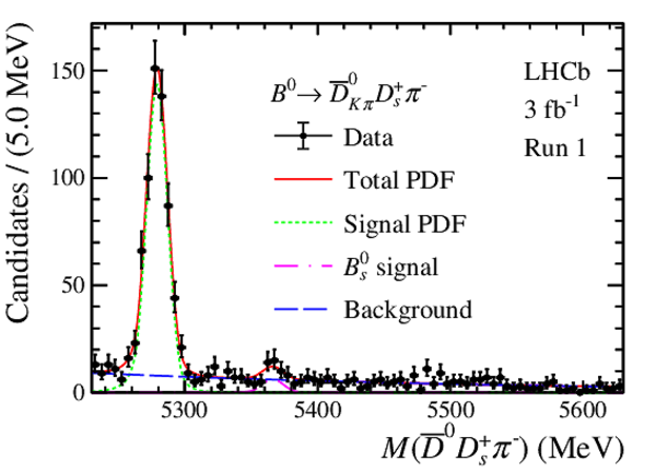
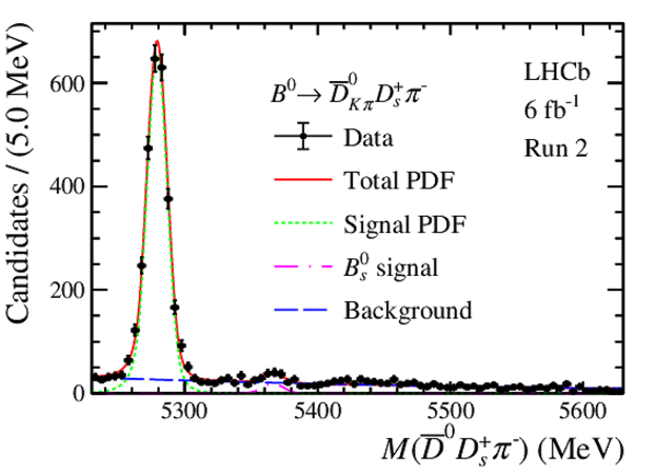
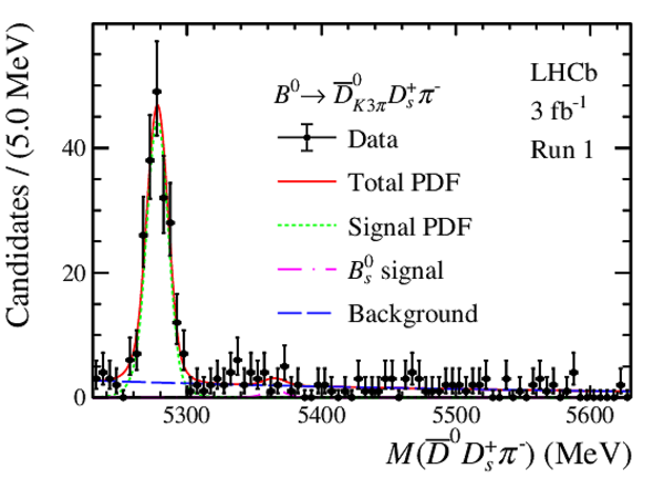
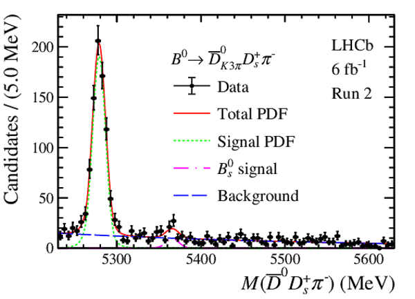
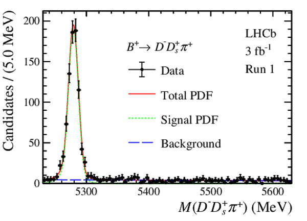
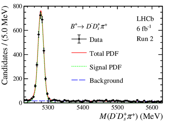
Invariant mass spectrum of the signal candidates, split by decay mode and run period. The data are overlaid with the results of the fit.

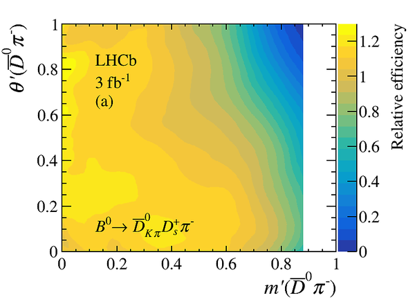
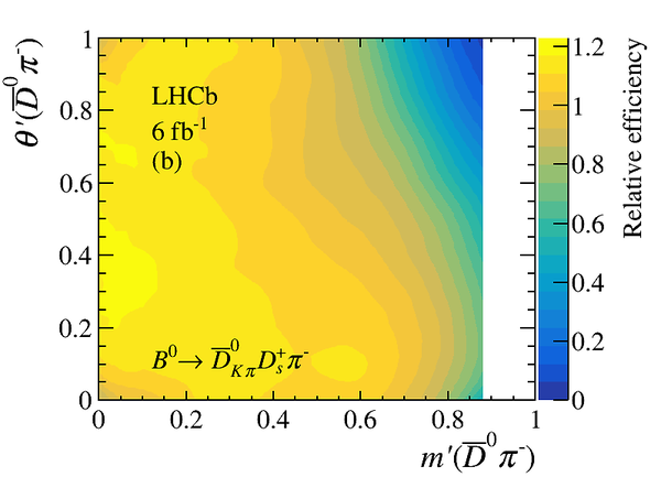
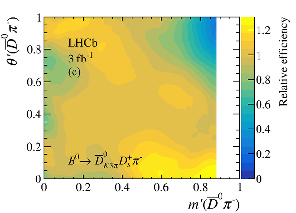
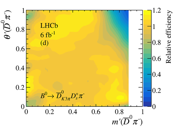
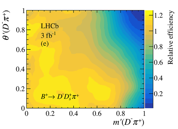
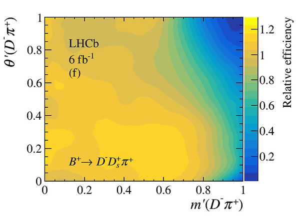
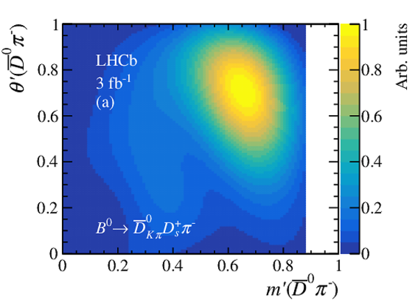
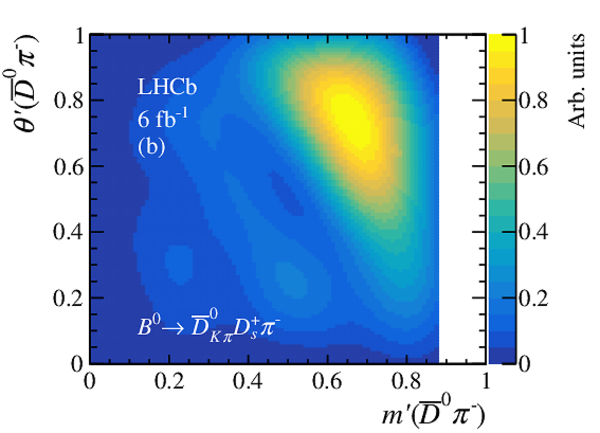
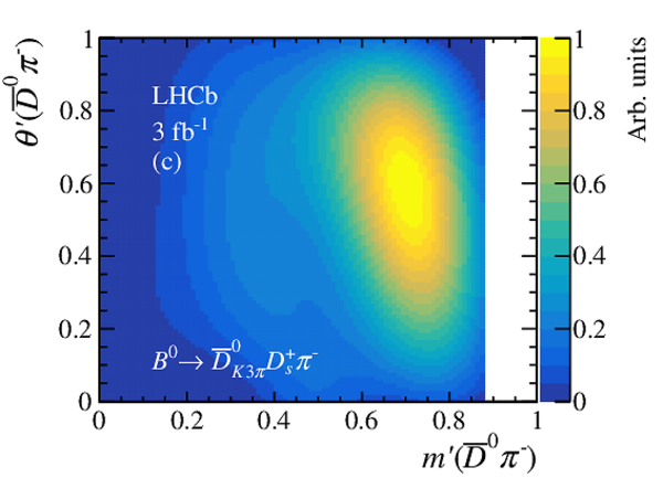
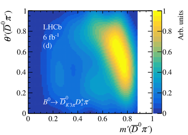
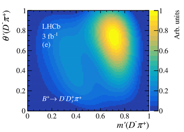
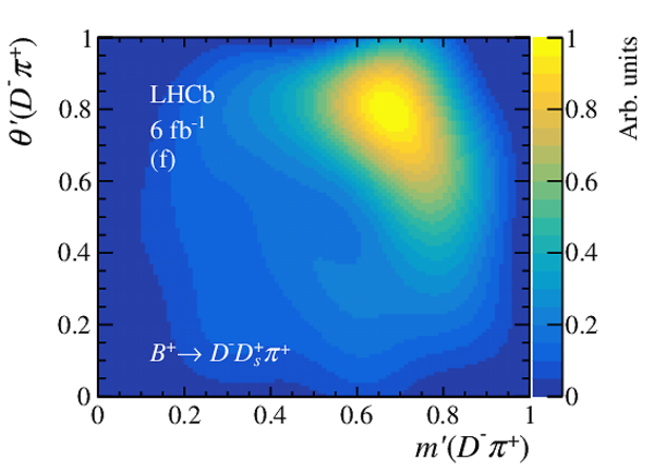
Signal efficiency maps for the $ B ^0 \rightarrow \overline{ D } {}^0 D ^+_ s \pi ^- $, $\overline{ D } {}^0 \rightarrow K ^+ \pi ^- $ decays in (a) Run 1 and (b) Run 2; $ B ^0 \rightarrow \overline{ D } {}^0 D ^+_ s \pi ^- $, $\overline{ D } {}^0 \rightarrow K ^+ \pi ^- \pi ^- \pi ^+ $ decays in (c) Run 1 and (d) Run 2; $ B ^+ \rightarrow D ^- D ^+_ s \pi ^+ $ decays in (e) Run 1 and (f) Run 2. White regions are caused by $ B ^0 \rightarrow D ^{*-} D ^+_ s $ veto.

Distributions of the SPD background shapes for the $ B ^0 \rightarrow \overline{ D } {}^0 D ^+_ s \pi ^- $, $\overline{ D } {}^0 \rightarrow K ^+ \pi ^- $ decays in (a) Run 1 and (b) Run 2; $ B ^0 \rightarrow \overline{ D } {}^0 D ^+_ s \pi ^- $, $\overline{ D } {}^0 \rightarrow K ^+ \pi ^- \pi ^- \pi ^+ $ decays in (c) Run 1 and (d) Run 2; $ B ^+ \rightarrow D ^- D ^+_ s \pi ^+ $ decays in (e) Run 1 and (f) Run 2. White regions are caused by $ B ^0 \rightarrow D ^{*-} D ^+_ s $ veto.

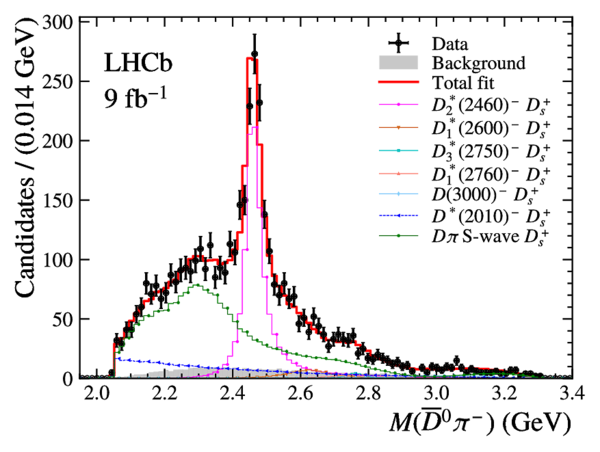
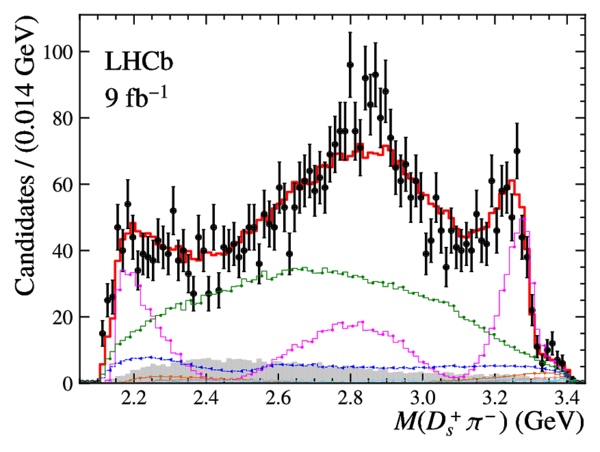
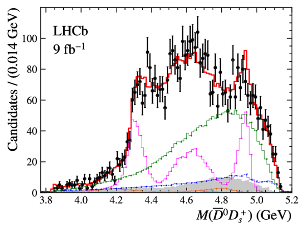
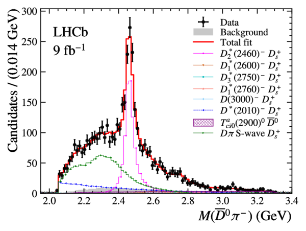
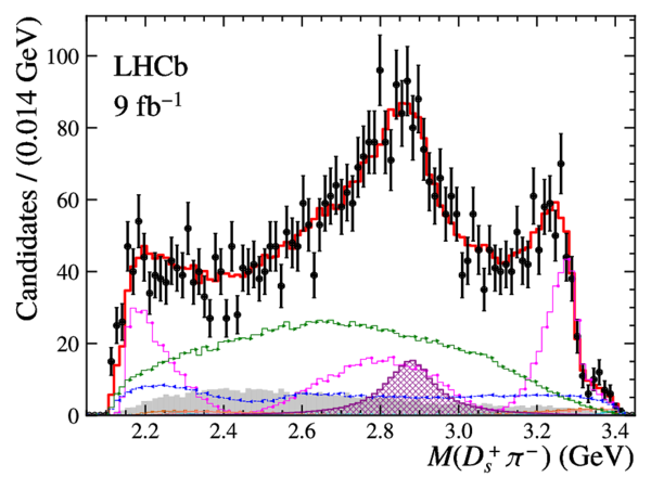
Invariant mass distributions (a) $M(\overline{ D } {}^0 \pi ^- )$, (b) $M( D ^+_ s \pi ^- )$ and (c) $M(\overline{ D } {}^0 D ^+_ s )$ for the $ B ^0 \rightarrow \overline{ D } {}^0 D ^+_ s \pi ^- $ candidates compared with the fit results with only $D\pi$ resonances.

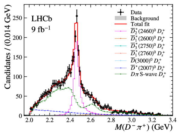
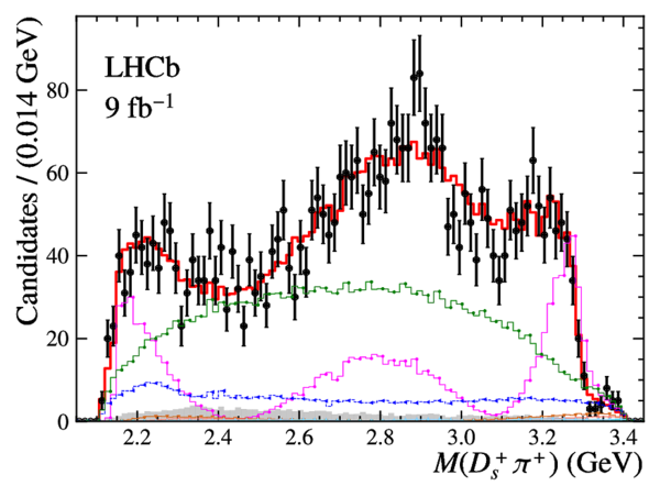
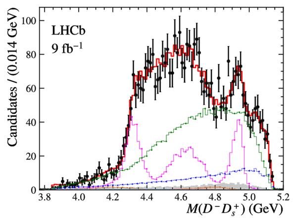
Invariant mass distributions of the (a) $M( D ^- \pi ^+ )$, (b) $M( D ^+_ s \pi ^+ )$ and (c) $M( D ^- D ^+_ s )$ for the $ B ^+ \rightarrow D ^- D ^+_ s \pi ^+ $ candidates compared with the fit results with only $D\pi$ resonances.

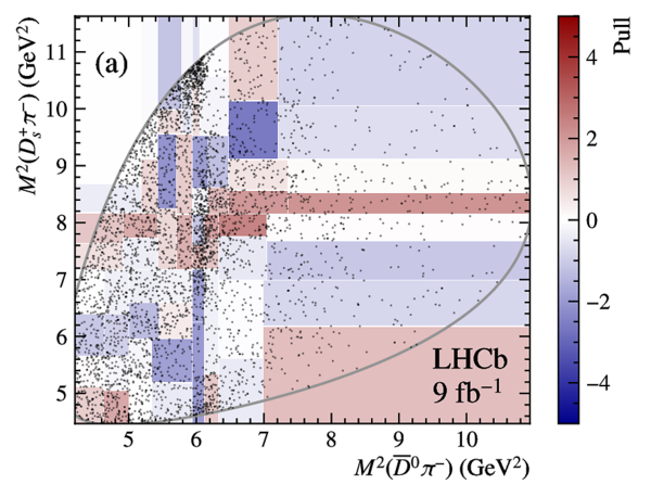
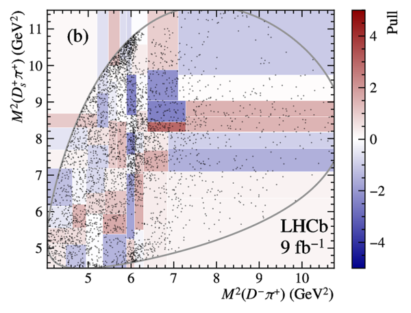
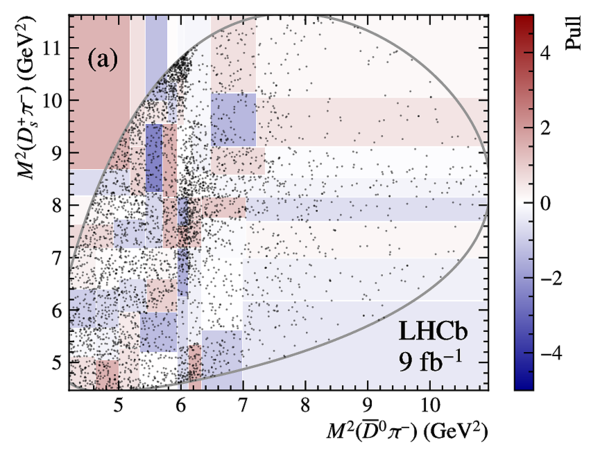
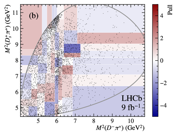
Two-dimensional pull plots of the fits to the (a) $ B ^0 \rightarrow \overline{ D } {}^0 D ^+_ s \pi ^- $ and (b) $ B ^+ \rightarrow D ^- D ^+_ s \pi ^+ $ samples.

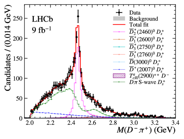
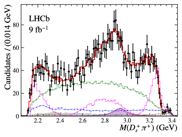
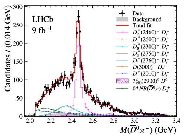
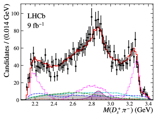
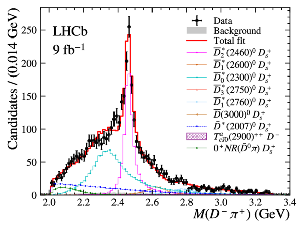
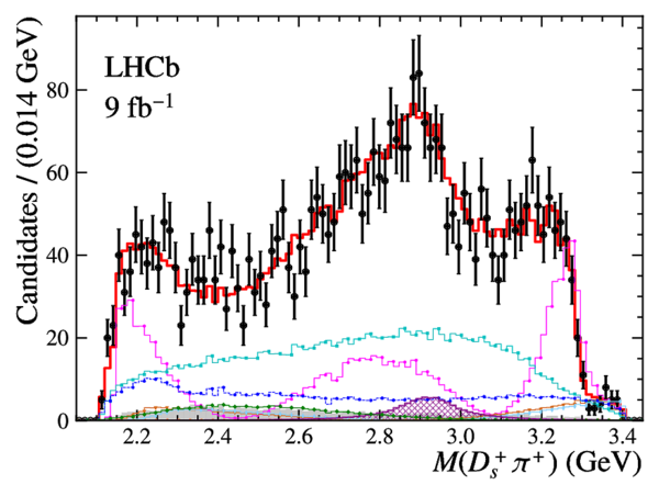
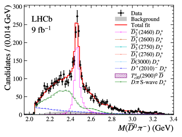
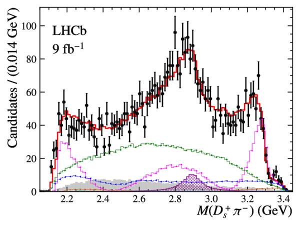
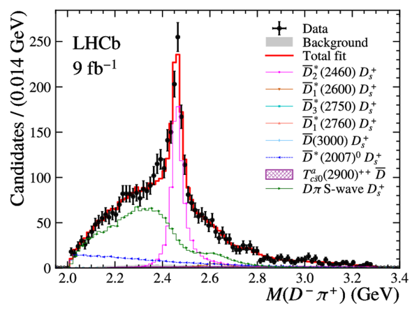
Projection of the fit result on (a) $M(D\pi)$ and (b) $M( D ^+_ s \pi)$ of $ B ^0 \rightarrow \overline{ D } {}^0 D ^+_ s \pi ^- $ decays after including the $ T^a_{c\bar{s}0}(2900)^0 $ state, and on (c) $M(D\pi)$ and (d) $M( D ^+_ s \pi)$ of $ B ^+ \rightarrow D ^- D ^+_ s \pi ^+ $ decays after including the $ T^a_{c\bar{s}0}(2900)^{++} $ state.

Two-dimensional pull plots of the fits to (a) $ B ^0 \rightarrow \overline{ D } {}^0 D ^+_ s \pi ^- $ and (b) $ B ^+ \rightarrow D ^- D ^+_ s \pi ^+ $ samples after including the $ T^a_{c\bar{s}0}(2900)^0$ and $ T^a_{c\bar{s}0}(2900)^{++}$ states.

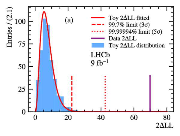
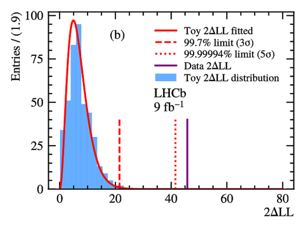
Significance tests for the new $D_s\pi$ states in the (a) $ B ^0 \rightarrow \overline{ D } {}^0 D ^+_ s \pi ^- $ and (b) $ B ^+ \rightarrow D ^- D ^+_ s \pi ^+ $ samples. The blue histogram is the distribution of $2\Delta{\rm LL}$ and the red solid curve shows the fitted $\chi^2$ PDF. The red dashed and dotted lines are the $2\Delta{\rm LL}$ values corresponding to $3 \sigma$ and $5 \sigma$, and the purple solid line is the $2\Delta{\rm LL}$ measured in the data.

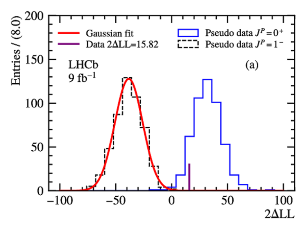
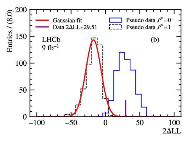
Spin analysis of (a) $ B ^0 \rightarrow \overline{ D } {}^0 D ^+_ s \pi ^- $ and (b) $ B ^+ \rightarrow D ^- D ^+_ s \pi ^+ $ decays. The blue solid and black dashed histograms are the distributions of the $2\Delta{\rm LL}$ for the pseudoexperiments generated based on the fit results with $0^+$ or $1^-$ $ D ^+_ s \pi$ exotic state, respectively. The purple vertical line shows the $2\Delta{\rm LL}$ value for the data fitted with the new $ D ^+_ s \pi$ exotic state under the $J^P=0^+$ and $J^P=1^-$ hypotheses. The red curve is the result of a fit to the black dashed histogram with a Gaussian function.

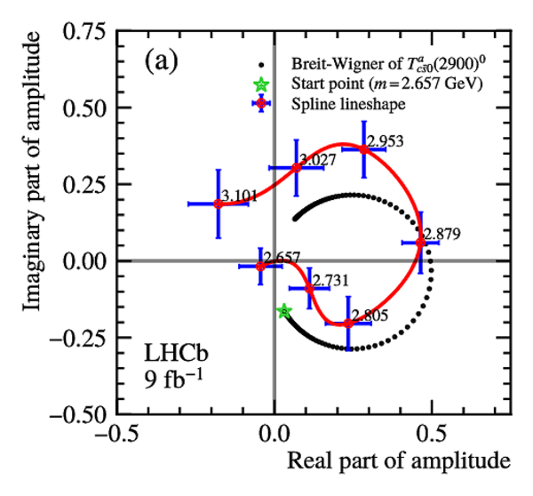
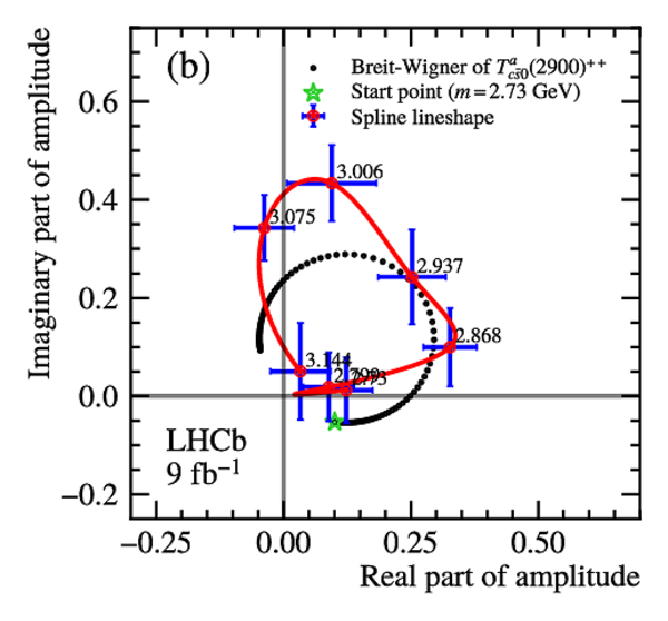
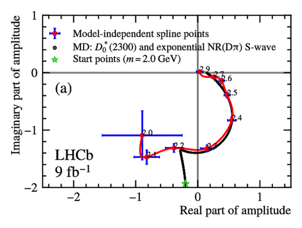
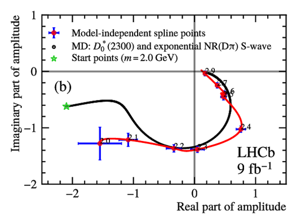
Argand diagrams of the (a) $ B ^0 \rightarrow \overline{ D } {}^0 D ^+_ s \pi ^- $ and (b) $ B ^+ \rightarrow D ^- D ^+_ s \pi ^+ $ decays. Black dots show the lineshape of the $ T^a_{c\bar{s}0}(2900)^0 $ and $ T^a_{c\bar{s}0}(2900)^{++} $ Breit--Wigner functions. The red solid line and blue error bars show the lineshape and fit results of spline $0^+$ $ D ^+_ s \pi$ model in $ T^a_{c\bar{s}0}(2900)^0 $ and $ T^a_{c\bar{s}0}(2900)^{++} $ mass region.

The MD description of the (a) $M(\overline{ D } {}^0 \pi ^- )$ and (b) $M( D ^+_ s \pi ^- )$ distributions for the $ B ^0 \rightarrow \overline{ D } {}^0 D ^+_ s \pi ^- $ decays.

The MD description of the (a) $M( D ^- \pi ^+ )$ and (b) $M( D ^+_ s \pi ^+ )$ distributions for the $ B ^+ \rightarrow D ^- D ^+_ s \pi ^+ $ decays.

Argand diagrams of the MD and qMI $0^+$ $D\pi$ components of the (a) $ B ^0 \rightarrow \overline{ D } {}^0 D ^+_ s \pi ^- $ and (b) $ B ^+ \rightarrow D ^- D ^+_ s \pi ^+ $ decays. The red solid line and blue error bars show the lineshape and fit results of qMI $0^+$ $D\pi$ spline model, while the black line is the lineshape of the MD $0^+$ $D\pi$ component.

Fit result of simultaneous $D\pi$ fit model, the (a) $M(D\pi)$ and (b) $M( D ^+_ s \pi)$ distributions of $ B ^0 \rightarrow \overline{ D } {}^0 D ^+_ s \pi ^- $ decays after including the $ T^a_{c\bar{s}0}(2900)^0 $ state; the (c) $M(D\pi)$ and (d) $M( D ^+_ s \pi)$ distributions of $ B ^+ \rightarrow D ^- D ^+_ s \pi ^+ $ decays after including the $ T^a_{c\bar{s}0}(2900)^{++} $ state.

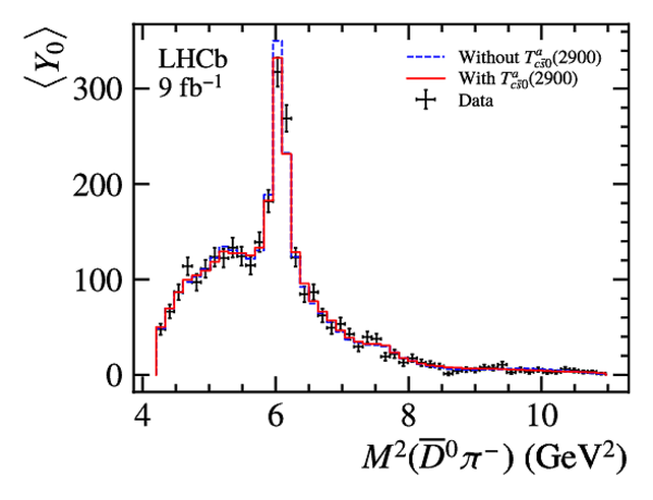
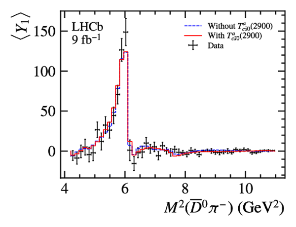
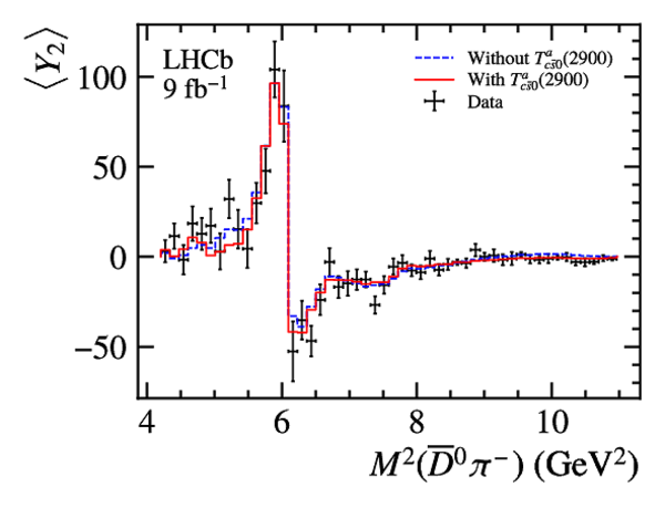
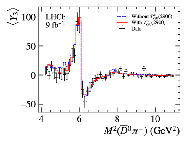
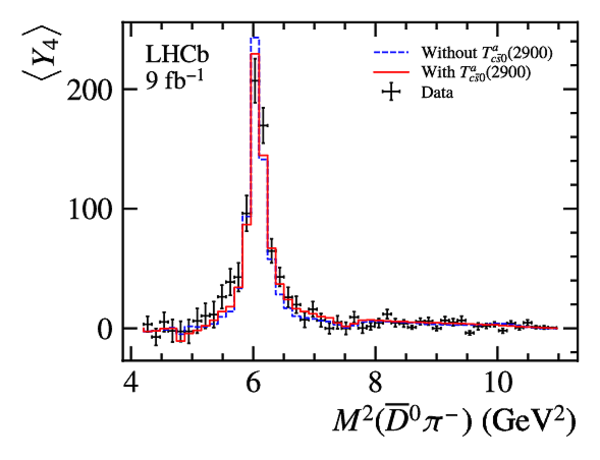
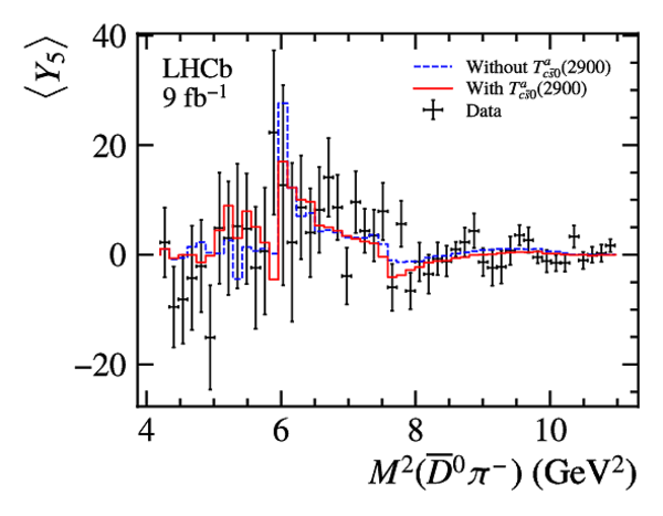
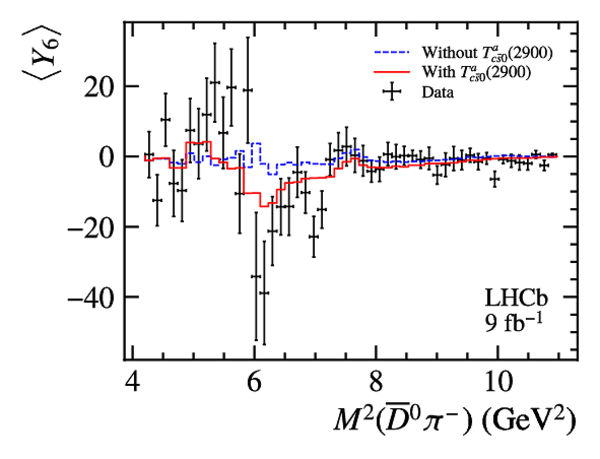
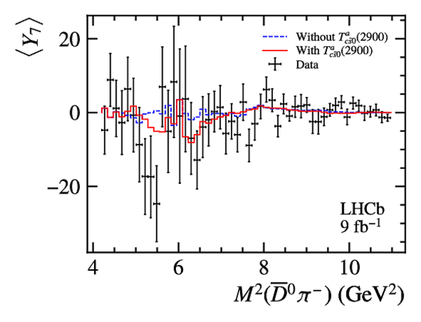
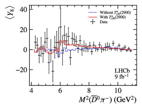
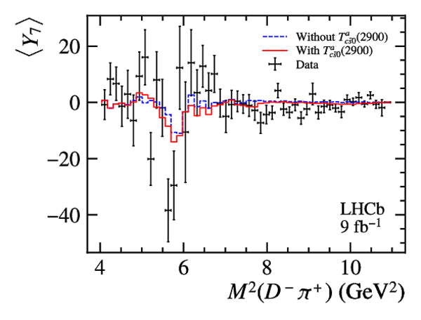
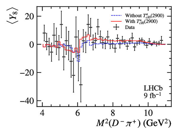
Moments analysis of $ B ^0 \rightarrow \overline{ D } {}^0 D ^+_ s \pi ^- $ on $M^2(\overline{ D } {}^0 \pi ^- )$. The black points indicate the data, while the blue and red histogram indicate the fit results without and with the $ T^a_{c\bar{s}0}(2900)$ states separately.

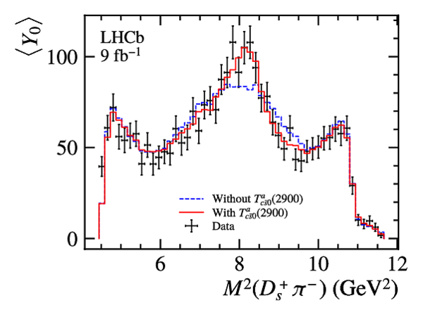
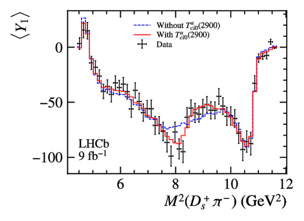
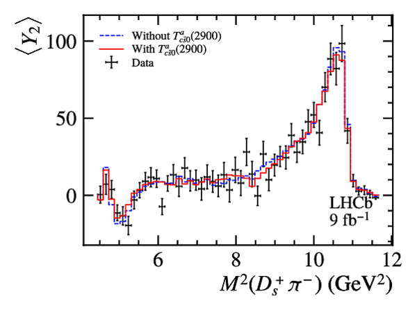
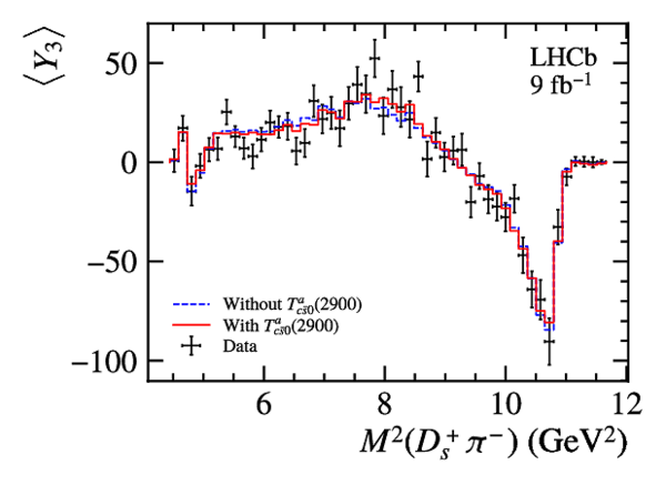
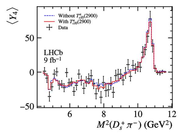
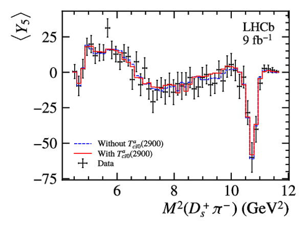
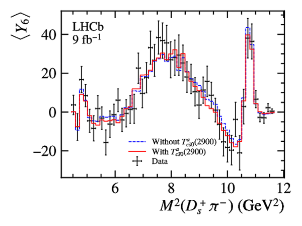
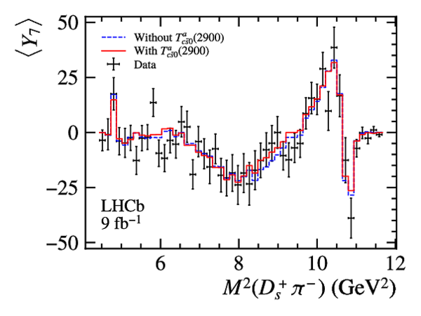
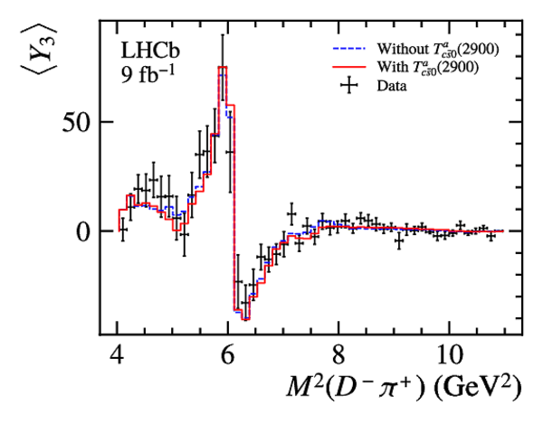
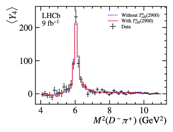
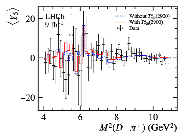
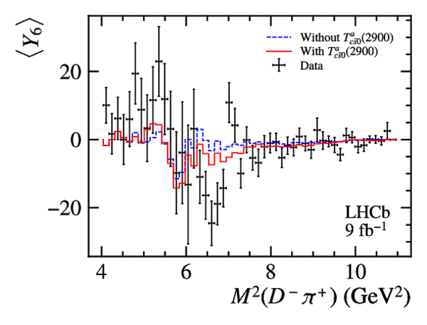
Moments analysis of $ B ^0 \rightarrow \overline{ D } {}^0 D ^+_ s \pi ^- $ on $M^2( D ^+_ s \pi ^- )$. The black points indicate the data, while the blue and red histogram indicate the fit results without and with the $ T^a_{c\bar{s}0}(2900)$ states separately.

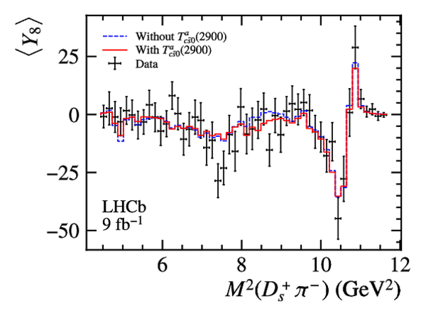
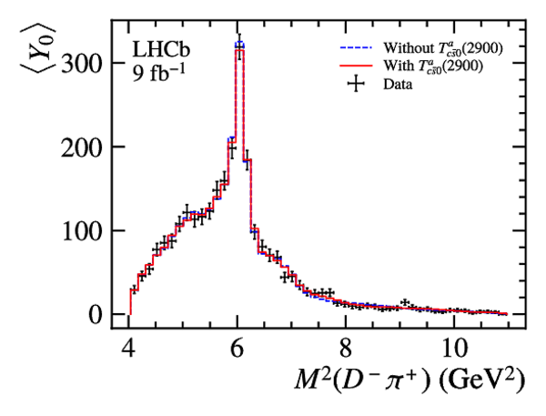
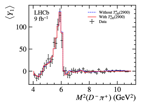
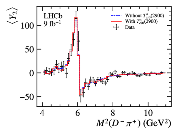
Moments analysis of $ B ^+ \rightarrow D ^- D ^+_ s \pi ^+ $ on $M^2( D ^- \pi ^+ )$. The black points indicate the data, while the blue and red histogram indicate the fit results without and with the $ T^a_{c\bar{s}0}(2900)$ states separately.

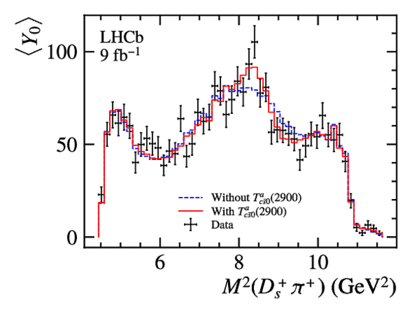
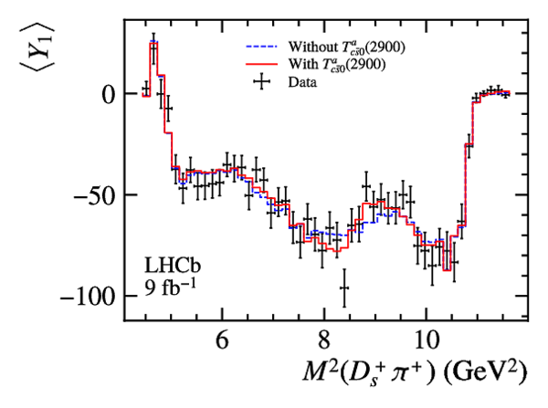
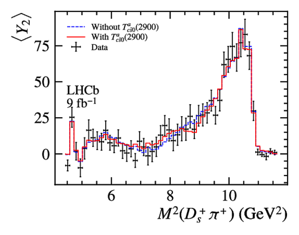
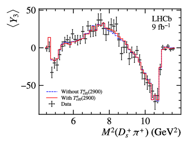
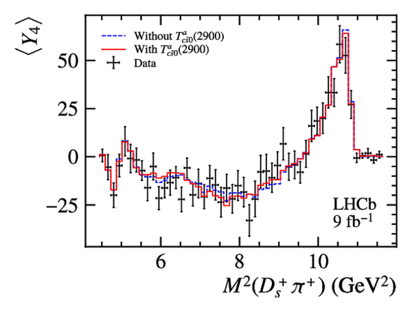
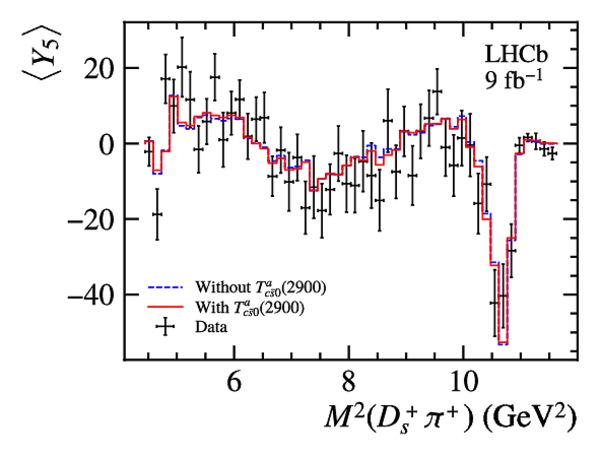
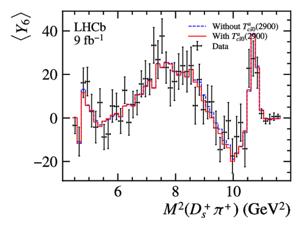
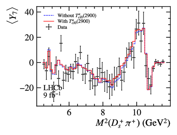
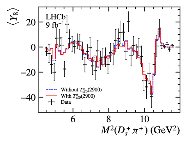
Moments analysis of $ B ^+ \rightarrow D ^- D ^+_ s \pi ^+ $ on $M^2( D ^+_ s \pi ^+ )$. The black points indicate the data, while the blue and red histogram indicate the fit results without and with the $ T^a_{c\bar{s}0}(2900)$ states separately.

Animated gif made out of all figures.

Results of the fit parameters of invariant mass fit to the data samples. The uncertainties shown are statistical.

Signal and background yields inside the $B$ mass signal window, together with the signal purity, split by run period and decay mode. The uncertainties shown are statistical.

Resonances expected in $ B ^0 \rightarrow \overline{ D } {}^0 D ^+_ s \pi ^- $ and $ B ^+ \rightarrow D ^- D ^+_ s \pi ^+ $ decays [7]. The masses and widths of resonances marked with \# are shared for both the charged and neutral isospin partners.

Masses and widths of the $ T^a_{c\bar{s}0}(2900)^0 $ and $ T^a_{c\bar{s}0}(2900)^{++} $ states. The values are corrected for biases. The first and second uncertainties are statistical and systematic, respectively.

Amplitude, phase, and fit fraction of each component in the $ B ^0 \rightarrow \overline{ D } {}^0 D ^+_ s \pi ^- $ fit result. The values are corrected for fit biases. The first and second uncertainties are statistical and systematic, respectively.

Amplitude, phase, and fit fraction of each component in the $ B ^+ \rightarrow D ^- D ^+_ s \pi ^+ $ fit result. The values are corrected for fit biases. The first and second uncertainties are statistical and systematic, respectively.

Tested fit models and the corresponding $\Delta \rm LL$ value.

Upper limit on the fit fractions of neutral and doubly charged $D_{s0}^*(2317)$ with different hypotheses at 90% C.L.

Masses, widths and fit fractions of the $ T^a_{c\bar{s}0}(2900)^0 $ and $ T^a_{c\bar{s}0}(2900)^{++} $ states obtained from the MD fit.

Masses and widths of the $ T^a_{c\bar{s}0}(2900)^0 $ and $ T^a_{c\bar{s}0}(2900)^{++} $ states. The values are corrected for biases as described in the text. The first and second uncertainties are statistical and systematic, respectively.

Amplitude, phase and fit fraction of each component in the simultaneous $D\pi$ fit model. The values are corrected based on the results of pseudoexperiments. The first and second uncertainties are the statistical and systematic, respectively.