Amplitude analysis of the $\Lambda_b^0\to pK^-\gamma$ decay

Information

LHCb-PAPER-2023-036
CERN-EP-2023-253
arXiv:2403.03710 [PDF]

(Submitted on 06 Mar 2024)
JHEP
Inspire 2765817

Tools

Get BibTex

Abstract

The resonant structure of the radiative decay $\Lambda_b^0\to pK^-\gamma$ in the region of proton-kaon invariant-mass up to 2.5 GeV$/c^2$ is studied using proton-proton collision data recorded at centre-of-mass energies of 7, 8, and 13 TeV collected with the LHCb detector, corresponding to a total integrated luminosity of 9 fb$^{-1}$. Results are given in terms of fit and interference fractions between the different components contributing to this final state. Only $\Lambda$ resonances decaying to $pK^-$ are found to be relevant, where the largest contributions stem from the $\Lambda(1520)$, $\Lambda(1600)$, $\Lambda(1800)$, and $\Lambda(1890)$ states.

Figures and captions

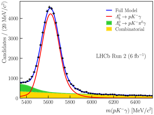
Distribution of the three-body invariant mass of the candidates in the (left) Run 1 and (right) Run 2 data sets. The results of the fits are overlaid.	Fig1a.pdf [167 KiB] HiDef png [278 KiB] Thumbnail [180 KiB] *.C file
	Fig1b.pdf [169 KiB] HiDef png [278 KiB] Thumbnail [175 KiB] *.C file
Distribution of the $\Lambda ^0_ b \rightarrow p K ^- \gamma $ candidates in the Dalitz plane, defined by $m^2_\Lambda ^0_ b ( p K ^- )$ and $m^2_\Lambda ^0_ b (p\gamma)$, after background-subtraction using the sPlot method for (left) Run 1 and (right) Run 2.	Fig2a.pdf [329 KiB] HiDef png [802 KiB] Thumbnail [508 KiB] *.C file
	Fig2b.pdf [337 KiB] HiDef png [1 MiB] Thumbnail [752 KiB] *.C file
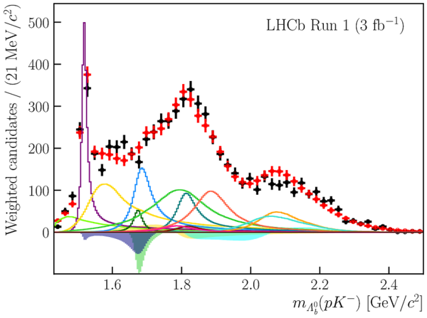
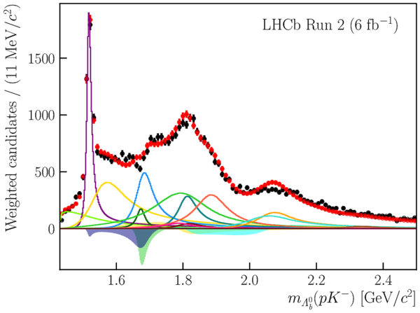
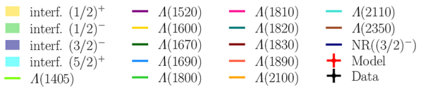
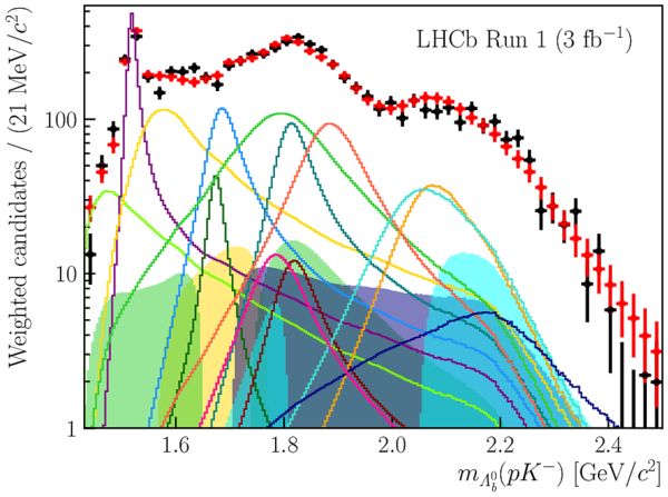
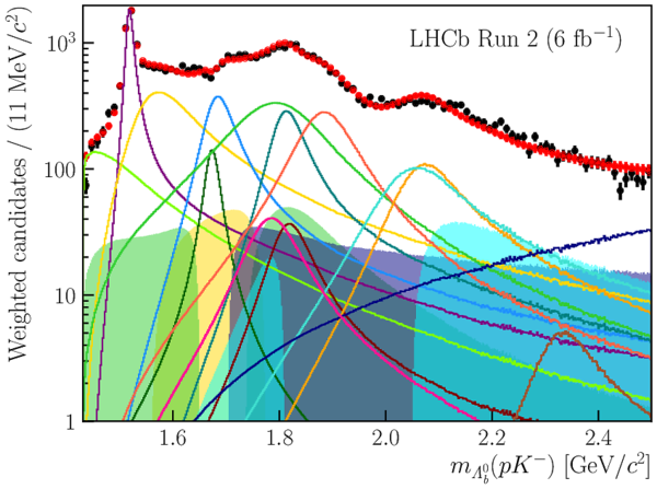
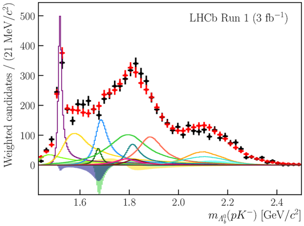
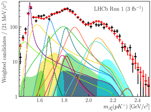
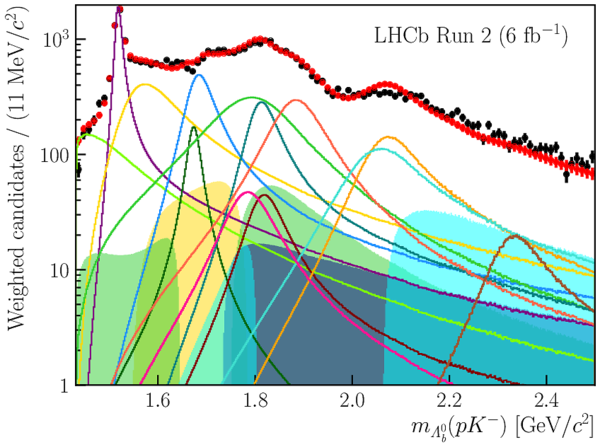
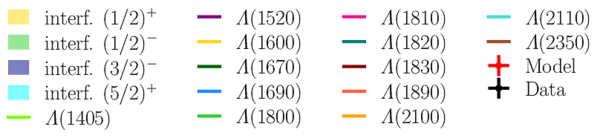
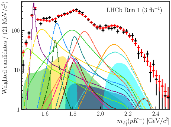
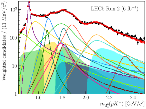
Background-subtracted distribution of the proton-kaon invariant-mass (black dots) for the (left) Run 1 and (right) Run 2 data samples. Also shown is a sample generated according to the result of a simultaneous fit of the reduced model to the data (red dots) and its components (lines) as well as the contributions due to interference between states with the same quantum numbers $J^P$ (shaded areas).	Fig3_l[..].pdf [222 KiB] HiDef png [114 KiB] Thumbnail [97 KiB] *.C file
	Fig3a.pdf [207 KiB] HiDef png [349 KiB] Thumbnail [194 KiB] *.C file
	Fig3b.pdf [254 KiB] HiDef png [360 KiB] Thumbnail [183 KiB] *.C file
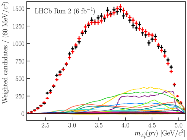
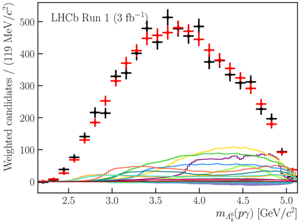
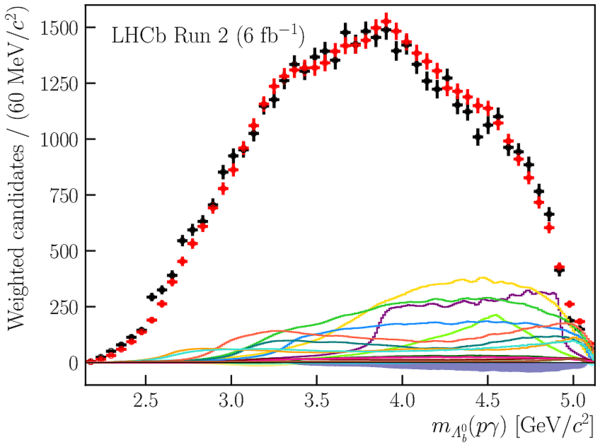
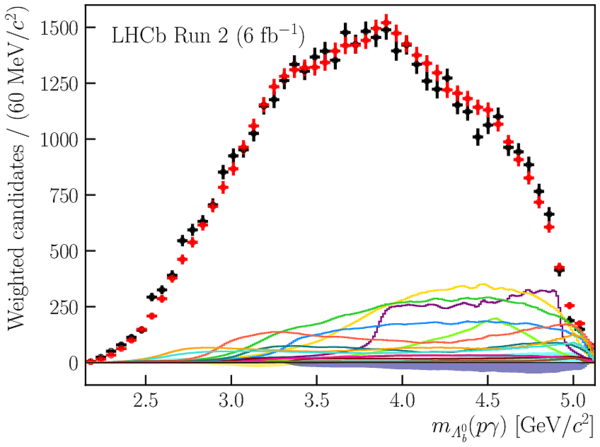
Background-subtracted distribution of the (top) proton-kaon and (bottom) proton-photon invariant-mass (black dots) for the (left) Run 1 and (right) Run 2 data samples. Also shown is a sample generated according to the result of a simultaneous fit of the default model to the data (red dots) and its components (lines) as well as the contributions due to interference between states with the same quantum numbers $J^P$ (shaded areas).	Fig4_l[..].pdf [222 KiB] HiDef png [114 KiB] Thumbnail [97 KiB] *.C file
	Fig4a.pdf [207 KiB] HiDef png [341 KiB] Thumbnail [190 KiB] *.C file
	Fig4b.pdf [255 KiB] HiDef png [353 KiB] Thumbnail [179 KiB] *.C file
	Fig4c.pdf [187 KiB] HiDef png [297 KiB] Thumbnail [185 KiB] *.C file
	Fig4d.pdf [212 KiB] HiDef png [406 KiB] Thumbnail [216 KiB] *.C file
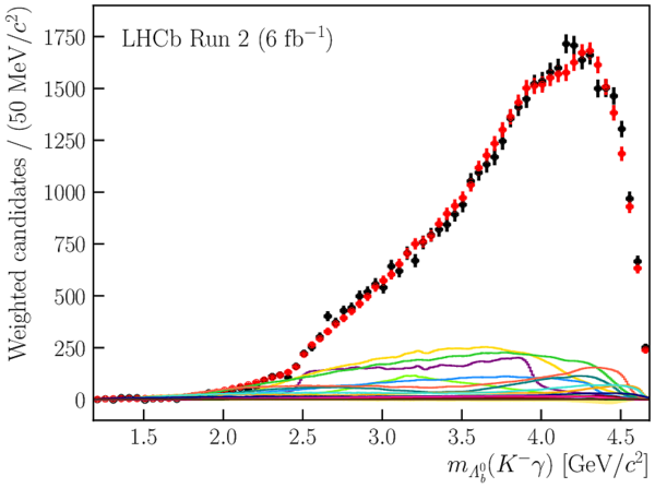
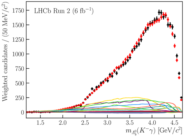
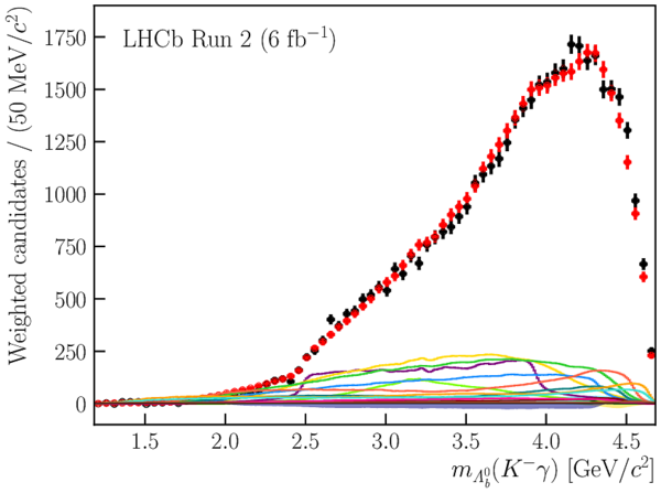
Background-subtracted distribution of (top) the kaon-photon invariant-mass and (bottom) the proton helicity angle (black dots) for the (left) Run 1 and (right) Run 2 data samples. Also shown is a sample generated according to the result of a simultaneous fit of the default model to the data (red dots) and its components (lines) as well as the contributions due to interference between states with the same quantum numbers $J^P$ (shaded areas). See Fig. 4 for the legend.	Fig5a.pdf [195 KiB] HiDef png [297 KiB] Thumbnail [171 KiB] *.C file
	Fig5b.pdf [232 KiB] HiDef png [358 KiB] Thumbnail [187 KiB] *.C file
	Fig5c.pdf [121 KiB] HiDef png [260 KiB] Thumbnail [155 KiB] *.C file
	Fig5d.pdf [144 KiB] HiDef png [350 KiB] Thumbnail [180 KiB] *.C file
Final results for the fit fractions and interference fit fractions. The vertical line separates the fit from the interference fit fractions. The error bars represent the different sources of uncertainty.	Fig6.pdf [138 KiB] HiDef png [351 KiB] Thumbnail [290 KiB] *.C file
Background-subtracted distribution of the proton-kaon invariant-mass (black dots) for the (left) Run 1 and (right) Run 2 data samples on a logarithmic scale. Also shown is a sample generated according to the result of a simultaneous fit of the default model to the data (red dots) and its components (lines) as well as the contributions due to interference between states with the same quantum numbers $J^P$ (shaded areas).	Fig7_l[..].pdf [188 KiB] HiDef png [114 KiB] Thumbnail [97 KiB] *.C file
	Fig7a.pdf [213 KiB] HiDef png [702 KiB] Thumbnail [368 KiB] *.C file
	Fig7b.pdf [290 KiB] HiDef png [977 KiB] Thumbnail [447 KiB] *.C file
Background-subtracted distribution of (top) the proton-photon invariant-mass, (middle) the kaon-photon invariant-mass, and (bottom) the proton helicity angle (black dots) for the (left) Run 1 and (right) Run 2 data samples. Also shown is a sample generated according to the result of a simultaneous fit of the reduced model to the data (red dots) and its components (lines) as well as the contributions due to interference between states with the same quantum numbers $J^P$ (shaded areas). See Fig. 3 for the legend.	Fig8a.pdf [186 KiB] HiDef png [304 KiB] Thumbnail [190 KiB] *.C file
	Fig8b.pdf [212 KiB] HiDef png [418 KiB] Thumbnail [221 KiB] *.C file
	Fig8c.pdf [195 KiB] HiDef png [308 KiB] Thumbnail [174 KiB] *.C file
	Fig8d.pdf [231 KiB] HiDef png [371 KiB] Thumbnail [192 KiB] *.C file
	Fig8e.pdf [121 KiB] HiDef png [255 KiB] Thumbnail [152 KiB] *.C file
	Fig8f.pdf [143 KiB] HiDef png [341 KiB] Thumbnail [180 KiB] *.C file
Background-subtracted distribution of (top three rows) the two-body invariant-masses and (bottom row) the proton helicity angle (black dots) for the (left) Run 1 and (right) Run 2 data samples. Also shown is a sample generated according to the result of a simultaneous fit of the second best model to the data (red dots) and its components (lines) as well as the contributions due to interference between states with the same quantum numbers $J^P$ (shaded areas). See Fig. 3 for the legend.	Fig9a.pdf [207 KiB] HiDef png [349 KiB] Thumbnail [192 KiB] *.C file
	Fig9b.pdf [254 KiB] HiDef png [358 KiB] Thumbnail [179 KiB] *.C file
	Fig9c.pdf [187 KiB] HiDef png [296 KiB] Thumbnail [187 KiB] *.C file
	Fig9d.pdf [213 KiB] HiDef png [412 KiB] Thumbnail [218 KiB] *.C file
	Fig9e.pdf [195 KiB] HiDef png [300 KiB] Thumbnail [172 KiB] *.C file
	Fig9f.pdf [232 KiB] HiDef png [365 KiB] Thumbnail [189 KiB] *.C file
	Fig9g.pdf [121 KiB] HiDef png [259 KiB] Thumbnail [155 KiB] *.C file
	Fig9h.pdf [143 KiB] HiDef png [337 KiB] Thumbnail [179 KiB] *.C file
Background-subtracted distribution of the proton-kaon invariant-mass (black dots) for the (left) Run 1 and (right) Run 2 data samples on a logarithmic scale. Also shown is a sample generated according to the result of a simultaneous fit of the reduced model to the data (red dots) and its components (lines) as well as the contributions due to interference between states with the same quantum numbers $J^P$ (shaded areas).	Fig10_[..].pdf [188 KiB] HiDef png [114 KiB] Thumbnail [97 KiB] *.C file
	Fig10a.pdf [212 KiB] HiDef png [662 KiB] Thumbnail [355 KiB] *.C file
	Fig10b.pdf [285 KiB] HiDef png [910 KiB] Thumbnail [426 KiB] *.C file
Background-subtracted distribution of the proton-kaon invariant-mass (black dots) for the (left) Run 1 and (right) Run 2 data samples on a logarithmic scale. Also shown is a sample generated according to the result of a simultaneous fit of the second best model to the data (red dots) and its components (lines) as well as the contributions due to interference between states with the same quantum numbers $J^P$ (shaded areas).	Fig11_[..].pdf [222 KiB] HiDef png [114 KiB] Thumbnail [97 KiB] *.C file
	Fig11a.pdf [213 KiB] HiDef png [679 KiB] Thumbnail [362 KiB] *.C file
	Fig11b.pdf [285 KiB] HiDef png [922 KiB] Thumbnail [432 KiB] *.C file
Animated gif made out of all figures.	PAPER-2023-036.gif Thumbnail

Tables and captions

List of well-established $\Lambda $ resonances and their properties as given in Ref. [29]. $J$ and $P$ are spin and parity of the resonance. The mass $m_0$ and width $\Gamma_0$ correspond to the Breit--Wigner parameters and are given in $\text{ Me V /}c^2$ and $\text{ Me V}$ respectively. The possible mass and width ranges, $\Delta m_0$ and $\Delta\Gamma_0$, are also given. If a measurement of mass and width is available, the uncertainties are given instead of a range. The columns $\sigma_{m_0}$ and $\sigma_{\Gamma_0}$ contain the $\sigma$ values used to estimate the systematic uncertainty related to the resonance parameters. The rightmost columns contain the allowed values of $l$ and $L$.	Table_1.pdf [77 KiB] HiDef png [129 KiB] Thumbnail [59 KiB] tex code
Systematic uncertainties on the fit fractions (top part of the table) and interference fit fractions (bottom part of the table). The values are given in %. The subscripts "BW", "radius", "amp.", and "res." refer to the systematic uncertainty due to fixing the resonance mass and width, fixing the radius of the hadrons, the choice of amplitude model, and the neglected resolution in the amplitude fit, respectively. The subscripts "finite", "acc.", and "kin." refer to the systematic uncertainties due to the finite simulation sample used to determine the acceptance model, the choice of acceptance model, and the kinematic reweighting respectively. The subscripts "$pK$", "$p\gamma$", and "comb." refer to the systematic uncertainty due to calculating the sWeights in bins of the proton-kaon invariant mass, the proton-gamma invariant mass, and the choice of model for the combinatorial background in the three-body invariant mass fit respectively.	Table_2.pdf [70 KiB] HiDef png [235 KiB] Thumbnail [106 KiB] tex code
Fit fractions (top) and interference fit fractions (bottom) determined using the amplitude model. The values are given in %. The uncertainties from internal and external sources, determined by the numerical convolution procedure are labelled $\sigma_\text{syst}^\text{internal}$ and $\sigma_\text{syst}^\text{external}$.	Table_3.pdf [85 KiB] HiDef png [254 KiB] Thumbnail [131 KiB] tex code
Magnitude, $\|A_{LS}\|$, and phase, $\arg(A_{LS})$, of the couplings at the best fit point of the default model for resonances $\Lambda (1405)$, $\Lambda (1520)$, $\Lambda (1600)$, $\Lambda (1670)$, $\Lambda (1690)$, $\Lambda (1800)$, $\Lambda (1810)$, and $\Lambda (1820)$.	Table_4.pdf [57 KiB] HiDef png [277 KiB] Thumbnail [137 KiB] tex code
Magnitude, $\|A_{LS}\|$, and phase, $\arg(A_{LS})$, of the couplings at the best fit point of the default model for resonances $\Lambda (1830)$, $\Lambda (1890)$, $\Lambda (2100)$, $\Lambda (2110)$, $\Lambda (2350)$, and the non-resonant component.	Table_5.pdf [70 KiB] HiDef png [246 KiB] Thumbnail [122 KiB] tex code
Statistical correlations between the observables in percent obtained from bootstrapping the data. In the interest of space, the $J^P$ specification of the nonresonant component of the best model, NR($\tfrac{3}{2}^-$), is dropped and the resonances are only referred to by their mass. A single mass refers to the fit fraction of a state, two masses refer to the interference fit fraction of the given combination.	Table_6.pdf [30 KiB] HiDef png [57 KiB] Thumbnail [22 KiB] tex code