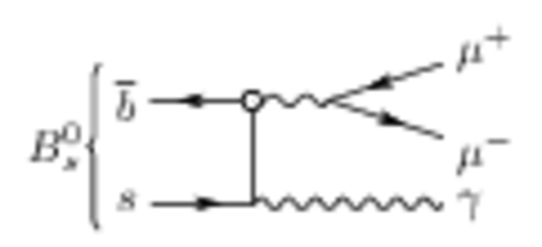
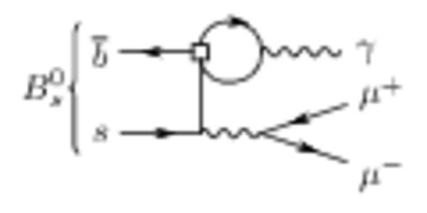
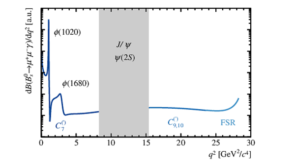
Illustration of the $q^2$ spectrum in $ B ^0_ s \rightarrow \mu ^+ \mu ^- \gamma $ decays from Refs. [16,3] for a photon energy larger than 50 $\text{ Me V /}c^2$ . The grey band corresponds to the excluded region dominated by $ B ^0_ s \rightarrow { J \mskip -3mu/\mskip -2mu\psi } \gamma$ and $ B ^0_ s \rightarrow \psi {(2S)} \gamma$ decays. The Wilson coefficients and the FSR are highlighted in the region of the spectrum where they are dominant. The magnitudes are chosen for illustrative purposes.

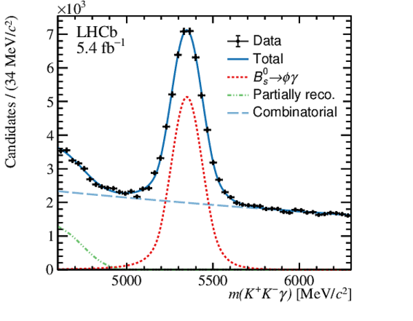
Mass distribution of $ B ^0_ s \rightarrow \phi \gamma $ candidates from data, used as control channel. The fit to the distribution is superimposed.

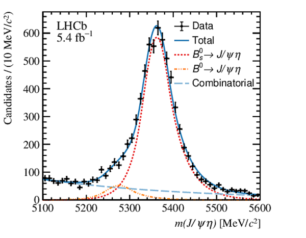
Mass distribution of $ B ^0_ s \rightarrow { J \mskip -3mu/\mskip -2mu\psi } \eta $ candidates from data, used as normalisation channel. The fit to the distribution is superimposed.

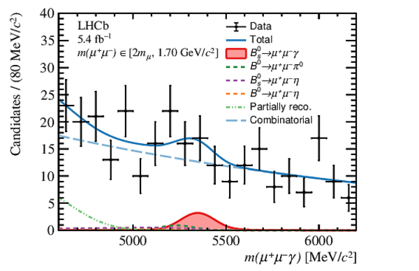
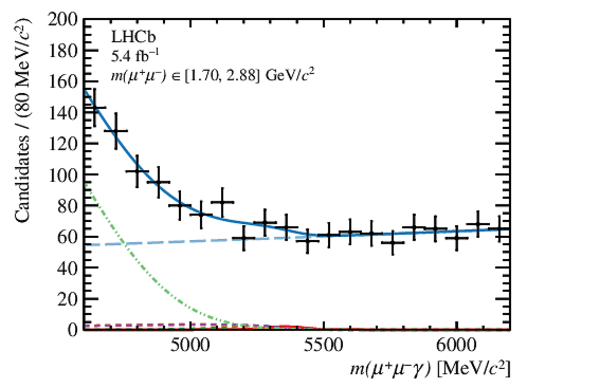
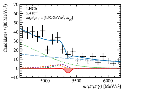
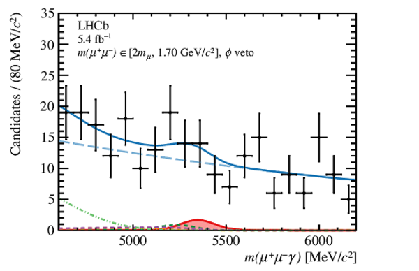
Mass distribution of signal candidates in regions of $q^2$, (top-left) bin I, (top-right) bin II, (bottom-left) bin III, and (bottom-right) $\phi $ -veto bin. The result of the fit is overlaid and the different components detailed in the legend.

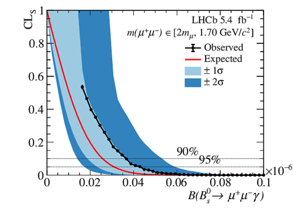
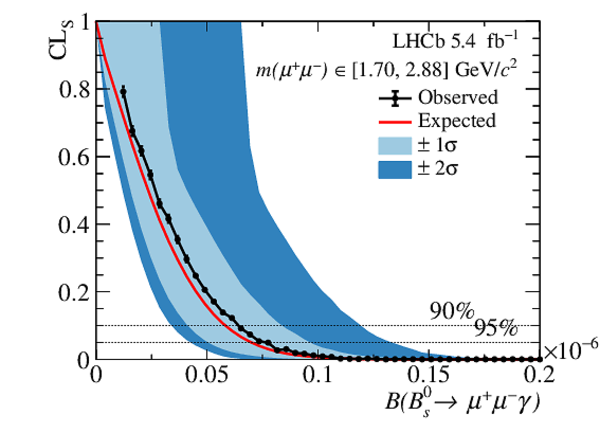
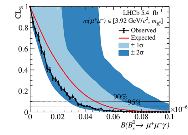
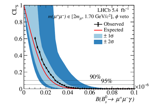
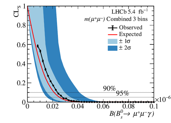
Results from the CL$_{\mathrm{s}}$ scan used to obtain the limit on $\mathcal{B} ( B ^0_ s \rightarrow \mu ^+ \mu ^- \gamma )$ in regions of $q^2$: (top-left) bin I, (top-right) bin II, (middle-left) bin III, (middle-right) bin I with $\phi $ veto, and (bottom) the whole $q^2$ range. The expected limit is shown by the red line and the 1$\sigma$ and 2$\sigma$ bands are shown as light blue and blue bands, respectively. The observed limit is shown as the solid black line. The two dashed lines intersecting with the observation indicate the limits at 90% and 95% CL for the upper and lower line, respectively.

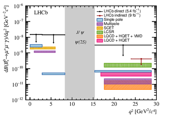
Differential branching fraction of the $ B ^0_ s \rightarrow \mu ^+ \mu ^- \gamma $ decay in intervals of $q^2$. The black arrows represent the limits set in this paper at 95% CL. The limit set in the high-$q^2$ region with the indirect method from the $ B ^0_ s \rightarrow \mu ^+ \mu ^- $ measurement at 95% CL is represented in red [18]. SM predictions using different form factor calculations are represented in (blue) Ref. [9], (violet) Ref. [10], (yellow) Ref. [11], (green) Ref. [12], (orange) Ref. [14,15], and (pink) Ref. [13].

Animated gif made out of all figures.

Mass range definition, predicted branching fraction, and the expected fraction of signal yield in the different $q^2$ bins as calculated in Ref. [9].

Efficiency ratios and single-event sensitivities, for each $q^2$ bin. The uncertainties on the efficiency ratios include the systematic uncertainties presented in Sec. 5.1. The uncertainties on $\alpha$ are the propagated uncertainties from $\mathcal{B} _\textrm{norm}$, $N_\textrm{norm}$ and $\epsilon_\text{norm}/\epsilon_{\text{sig}}$.