Definition of the helicity angles in the (a) $ B ^+ \rightarrow \overline{ D } ^{**0}(\rightarrow D ^{*-} \pi ^+ ) D ^+_ s $, (b) $ B ^+ \rightarrow D ^{*-} T_{c\bar{s}}^{++}(\rightarrow D ^+_ s \pi ^+ )$, and (c) $ B ^+ \rightarrow \overline{T}_{c\bar{c} s}^0(\rightarrow D ^{*-} D ^+_ s )\pi ^+ $ decay chains. Here $T_{c\bar{s}}^{++}$ and $\overline{T}_{c\bar{c} s}^0$ are the hypothetical tetraquark-like states decaying to $ D ^+_ s \pi ^+ $ and $ D ^{*-} D ^+_ s $ final states, respectively, following the nomenclature suggested in Ref. [18].

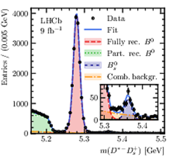
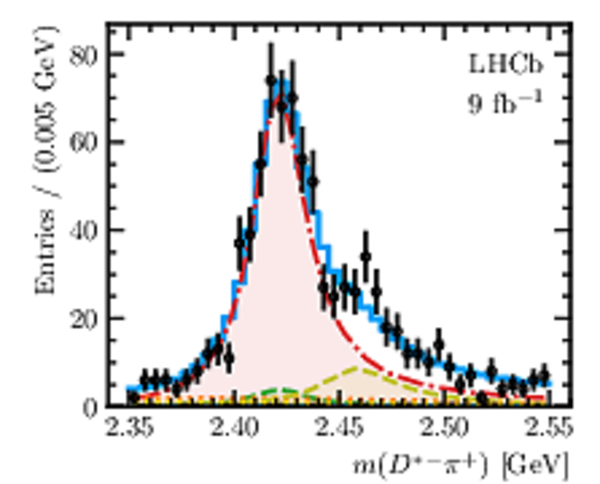
Invariant-mass distributions of (a) $ D ^{*-} D ^+_ s $ and (b) $ D ^{*-} D ^+_ s \pi ^+ $ combinations and the results of the fits used to obtain the yields of the $ B ^0 \rightarrow D ^{*-} D ^+_ s $, $ B ^+ \rightarrow D ^{*-} D ^+_ s \pi ^+ $ and $ B ^+ \rightarrow D ^{*-} D ^{*+}_ s \pi ^+ $ decays. The inset in the plot (a) shows a zoomed region with the contribution of the $ B ^0_ s \rightarrow D ^{*-} D ^+_ s $ decay component.

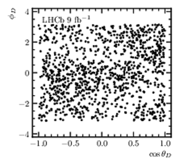
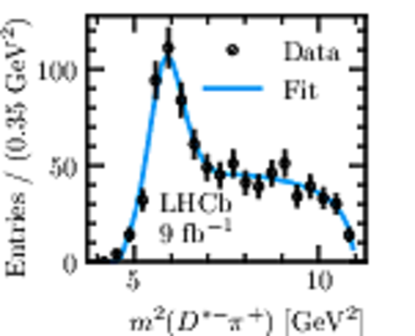
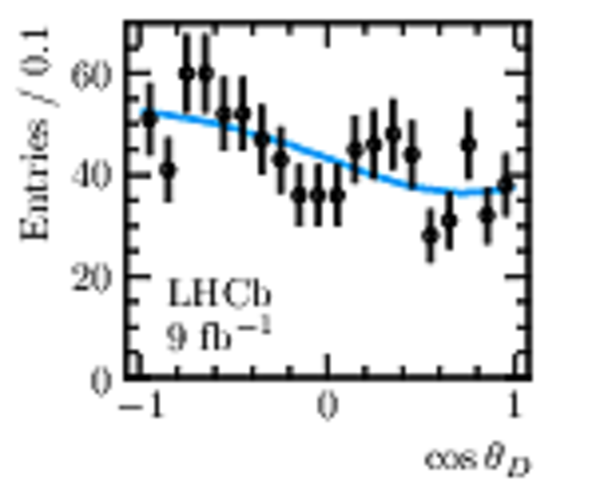
Distribution of $ B ^+ \rightarrow D ^{*-} D ^+_ s \pi ^+ $ candidates in data: (a) projection onto the Dalitz plot variables $m^2( D ^{*-} \pi ^+ )$ and $m^2( D ^+_ s \pi ^+ )$, (b) projection onto angular variables $\cos\theta_D$ and $\phi_D$ . The solid red line indicates the phase-space boundaries.

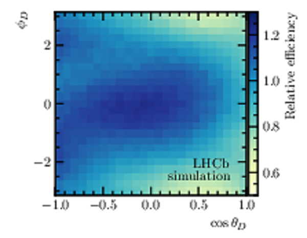
Projections of the $ B ^+ \rightarrow D ^{*-} D ^+_ s \pi ^+ $ efficiency profile averaged over trigger categories for (a,c) Run 1 and (b,d) Run 2 onto (a,b) $m^2( D ^{*-} \pi ^+ )$ and $m^2( D ^+_ s \pi ^+ )$ pair, and (c,d) $\phi_D$ and $\cos\theta_D$ pair.

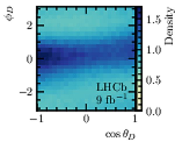
(a--e) One-dimensional projections of the distribution of $ B ^+ \rightarrow D ^{*-} D ^+_ s \pi ^+ $ candidates in the invariant mass range $5.31<m( D ^{*-} D ^+_ s \pi ^+ )<5.60$ $\text{ Ge V}$ (upper $ B ^+ $ invariant-mass sideband), results of its density estimated with ANN, and, except for (a), results of the extrapolation of its density to the signal region with $m( D ^{*-} D ^+_ s \pi ^+ ) = m_{ B ^+ }$. (f--i) Two-dimensional projections of the estimated density of $ B ^+ \rightarrow D ^{*-} D ^+_ s \pi ^+ $ candidates in the upper $ B ^+ $ mass sideband.

(a--d) One-dimensional projections of the distribution of $ B ^+ \rightarrow D ^{*-} D ^+_ s \pi ^+ $ candidates in the $ D ^+_ s $ sideband region and the results of its density estimation using ANN. (e, f) Two-dimensional projections of the estimated non-$ D ^+_ s $ background density.

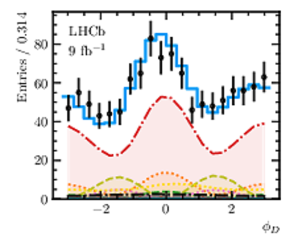
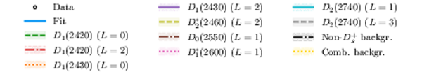
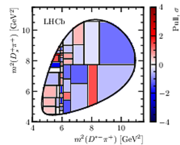
Results of the fit of the $ B ^+ \rightarrow D ^{*-} D ^+_ s \pi ^+ $ distribution with the baseline model. Figures (a) and (b) show the $m( D ^{*-} \pi ^+ )$ projection, with (a) zoomed in to illustrate the contributions from all the resonances while (b) shows the projection near the $D_1(2420)$ resonance. The $m( D ^+_ s \pi ^+ )$, $m( D ^{*-} D ^+_ s )$, $\cos\theta_{D}$ and $\phi_{D}$ projections are shown in (c), (d), (e) and (f), respectively.

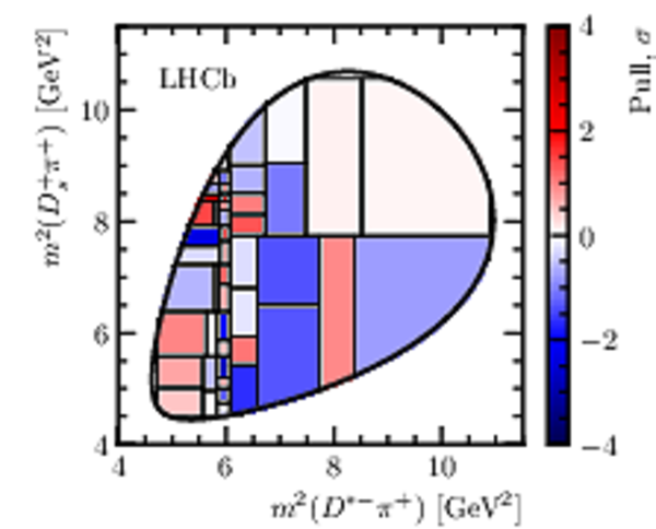
Pulls of the $ B ^+ \rightarrow D ^{*-} D ^+_ s \pi ^+ $ Dalitz-plot distribution for the fits with (a) the baseline model and (b) the model including $ D ^+_ s \pi ^+ $ components.

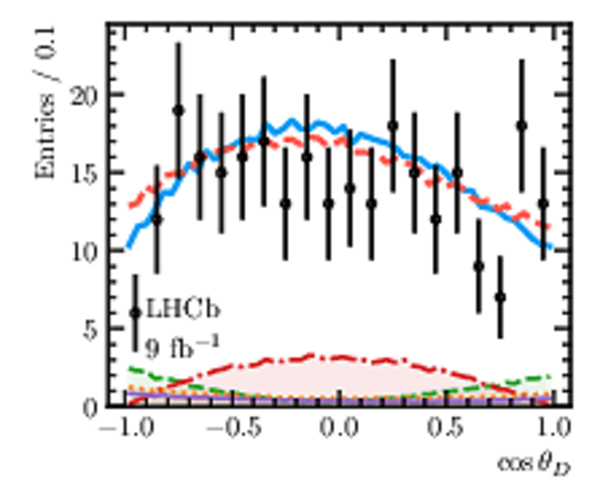
Comparison of the fit results of the $ B ^+ \rightarrow D ^{*-} D ^+_ s \pi ^+ $ distribution with the baseline model and with the model that includes $ D ^+_ s \pi ^+ $ components. The $m( D ^{*-} \pi ^+ )$, $m( D ^+_ s \pi ^+ )$, $m( D ^{*-} D ^+_ s )$, $\cos\theta_{D}$ and $\phi_{D}$ projections are shown in (a), (b), (c), (d) and (e), respectively. The requirement $m( D ^{*-} \pi ^+ )>2.5\text{ Ge V} $ is applied to the distributions shown in plots (b)--(e).

Animated gif made out of all figures.

The angular dependencies for the $ B ^+ \rightarrow \overline{ D } ^{**0}(\rightarrow D ^{*-} \pi ^+ ) D ^+_ s $ partial-wave terms $\mathcal{H}_n^{( D ^* \pi)}$.

The angular dependencies for the $ B ^+ \rightarrow D ^{*-} T_{c\bar{s}}^{++}(\rightarrow D ^+_ s \pi ^+ )$ partial-wave terms $\mathcal{H}_n^{( D _s\pi)}$.

Yields of signal and background components for the $ D ^{*-} D ^+_ s $ invariant-mass fit in range 5.15--5.60 $\text{ Ge V}$ .

Yields of signal and background components for the $ D ^{*-} D ^+_ s \pi ^+ $ invariant-mass fit in range 4.80--5.60 $\text{ Ge V}$ and in the signal box $|m( D ^{*-} D ^+_ s \pi ^+ )-m_{ B ^+ }|<30\text{ Me V} $.

Resonances considered in the baseline amplitude model and their parameters.

Fit fractions (in %) for the components of the $ B ^+ \rightarrow D ^{*-} D ^+_ s \pi ^+ $ amplitude. The first uncertainty is statistical, the second is systematic, and the third is the uncertainty related to the amplitude model.

Relative systematic uncertainties on the $\mathcal{R}^{(*)}$ measurements.

Fit results for the baseline and selected alternative $ B ^+ \rightarrow D ^{*-} D ^+_ s \pi ^+ $ amplitude models.

Fitted complex values $f_i$ of the $1^+$ S-wave amplitudes at the spline knots of the QMI model.

Absolute systematic uncertainties on the fit parameters and fit fractions for the baseline model

Absolute systematic uncertainties on the fit parameters and fit fractions for the baseline model (continued)