

Compact Muon Solenoid
LHC, CERN
| CMS-PAS-FTR-18-009 | ||
| Search for ${\text{t}\overline{\text{t}}}$ resonances at the HL-LHC and HE-LHC with the Phase-2 CMS detector | ||
| CMS Collaboration | ||
| November 2018 | ||
| Abstract: A search for a heavy resonance decaying into a ${\text{t}\overline{\text{t}}}$ pair is presented using the upgraded Phase-2 CMS detector design at the High-Luminosity LHC (HL-LHC) and High-Energy LHC (HE-LHC), with center-of-mass energies of 14 and 27 TeV, respectively, and integrated luminosities of 3 and 15 ab$^{-1}$. Two distinct final states with either a single lepton or no leptons are considered. Jet substructure techniques and top quark identification algorithms are used for the object reconstruction. At the HL-LHC (HE-LHC), the production of a Randall-Sundrum gluon can be excluded at 95% confidence level with a mass up to 6.6 (10.7) TeV or can be discovered at 5$\sigma$ significance with a mass up to 5.7 (9.4) TeV. | ||
| Links: CDS record (PDF) ; inSPIRE record ; CADI line (restricted) ; | ||
| Figures | |
png pdf |
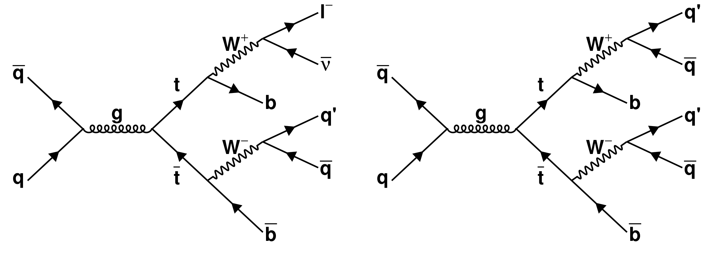
Figure 1:
Leading order Feynman diagrams showing pair production and decays of top quark with (left) single-lepton and (right) fully hadronic final states. |
png pdf |
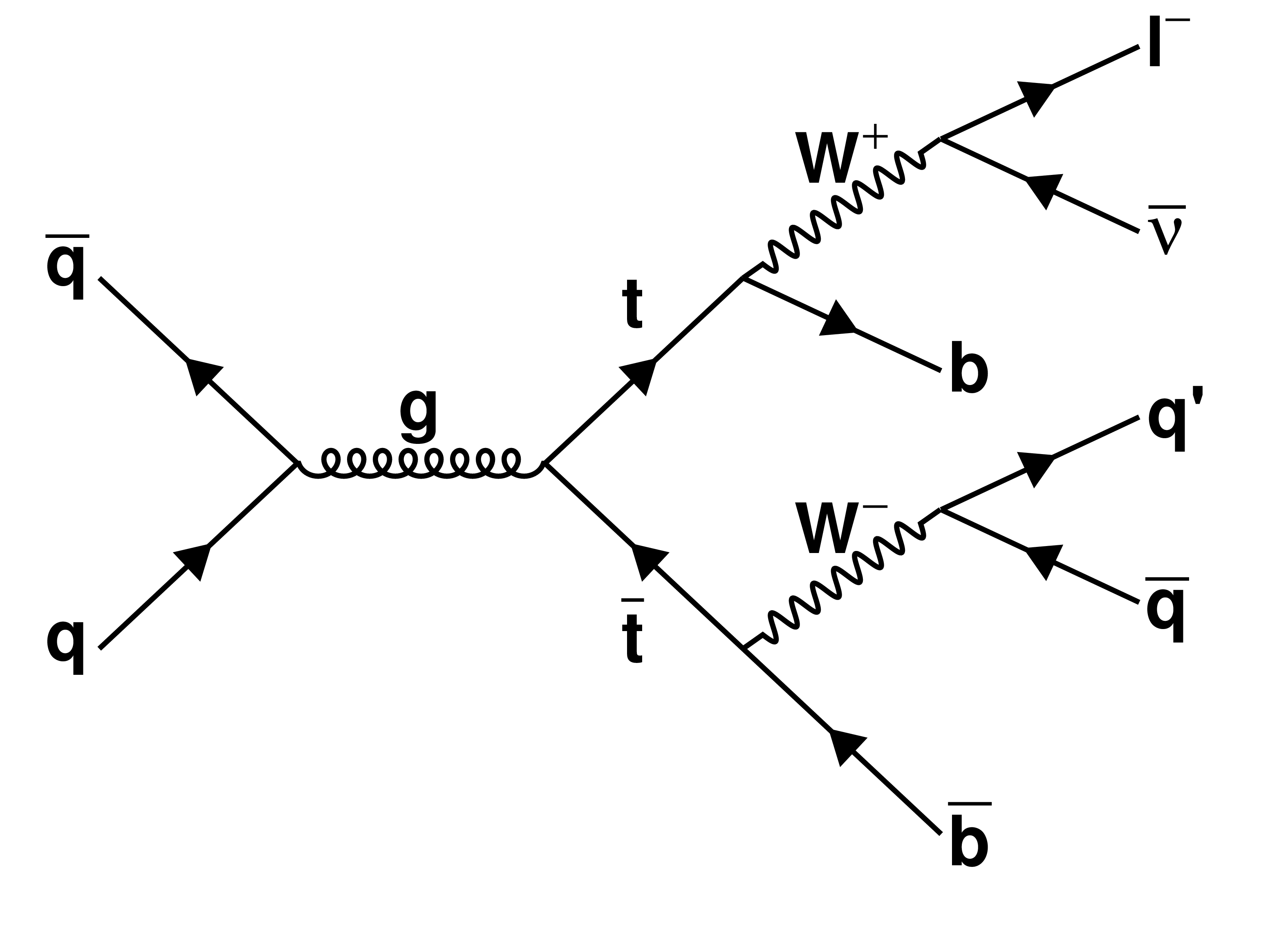
Figure 1-a:
Leading order Feynman diagrams showing pair production and decays of top quark with (left) single-lepton and (right) fully hadronic final states. |

png pdf |
Figure 1-b:
Leading order Feynman diagrams showing pair production and decays of top quark with (left) single-lepton and (right) fully hadronic final states. |
png pdf |
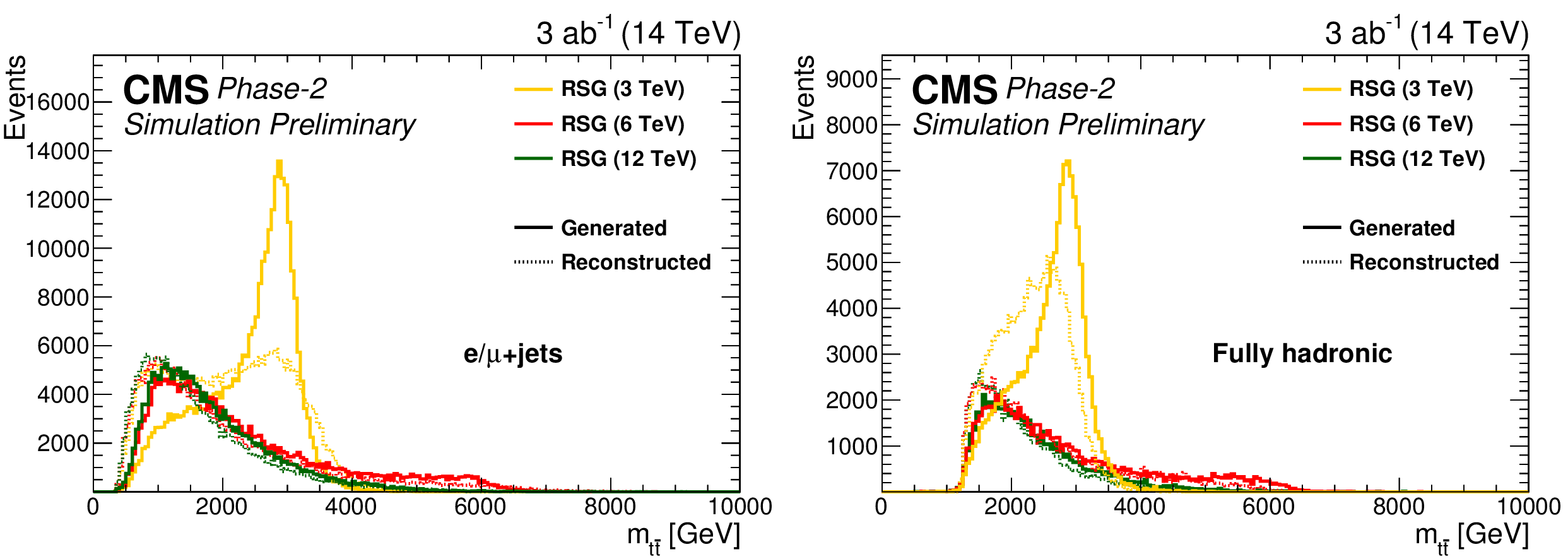
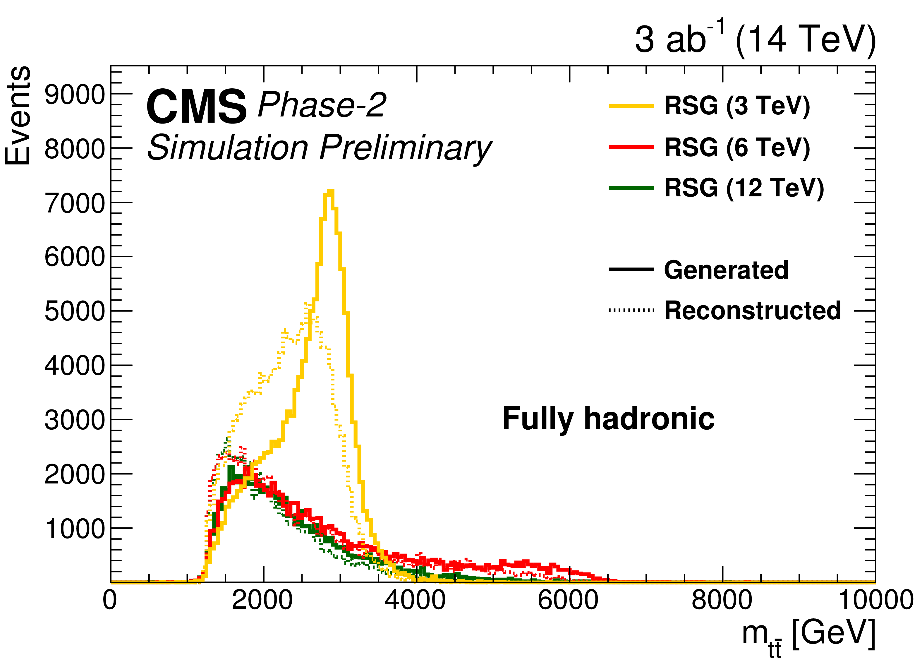
Figure 2:
The generated and reconstructed RSG mass distributions in the (left) single-lepton and (right) fully hadronic final states. The distributions are shown after the full event selection in each final state, as described in Sections xxxxx and yyyyy. |
png pdf |
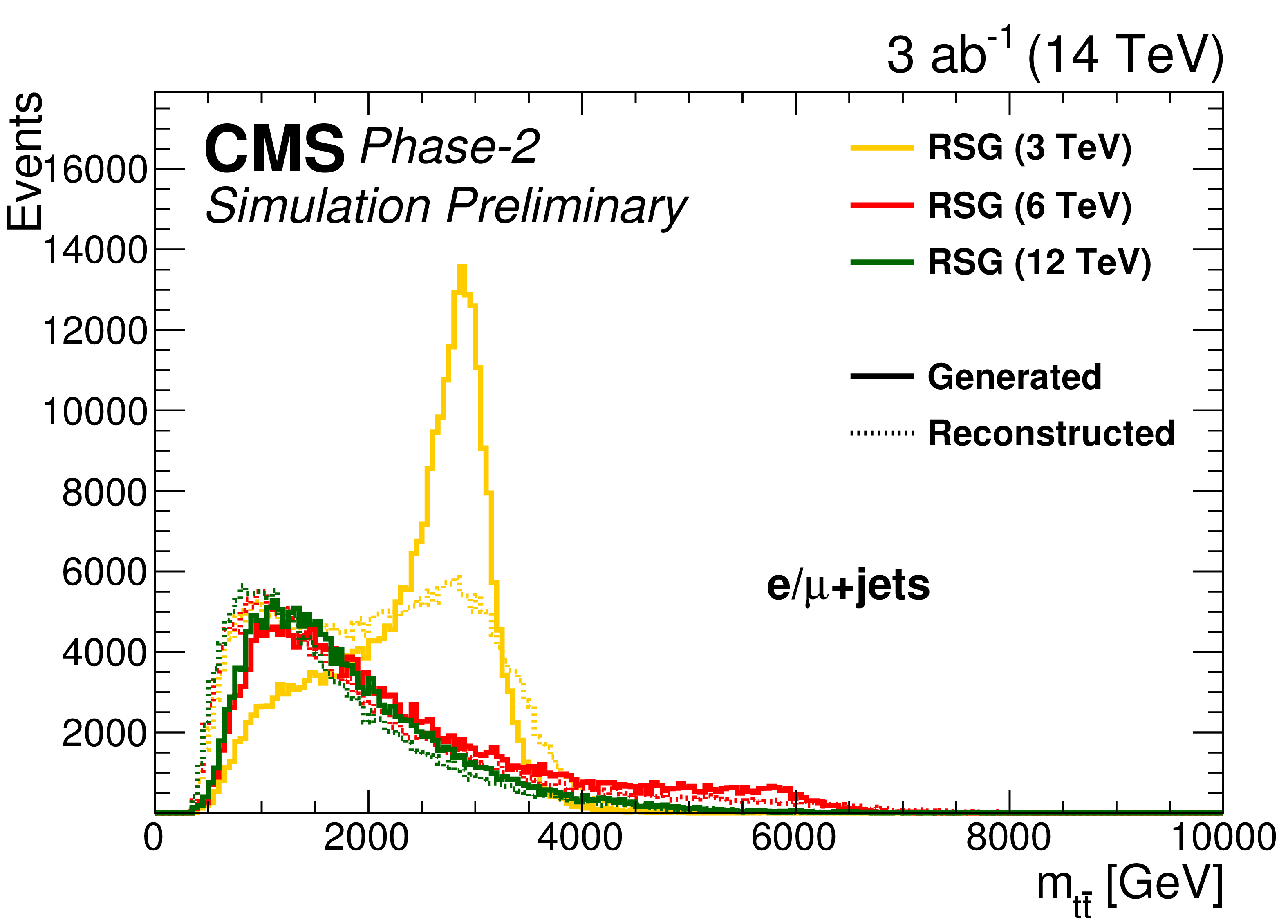
Figure 2-a:
The generated and reconstructed RSG mass distributions in the (left) single-lepton and (right) fully hadronic final states. The distributions are shown after the full event selection in each final state, as described in Sections xxxxx and yyyyy. |
png pdf |
Figure 2-b:
The generated and reconstructed RSG mass distributions in the (left) single-lepton and (right) fully hadronic final states. The distributions are shown after the full event selection in each final state, as described in Sections xxxxx and yyyyy. |
png pdf |
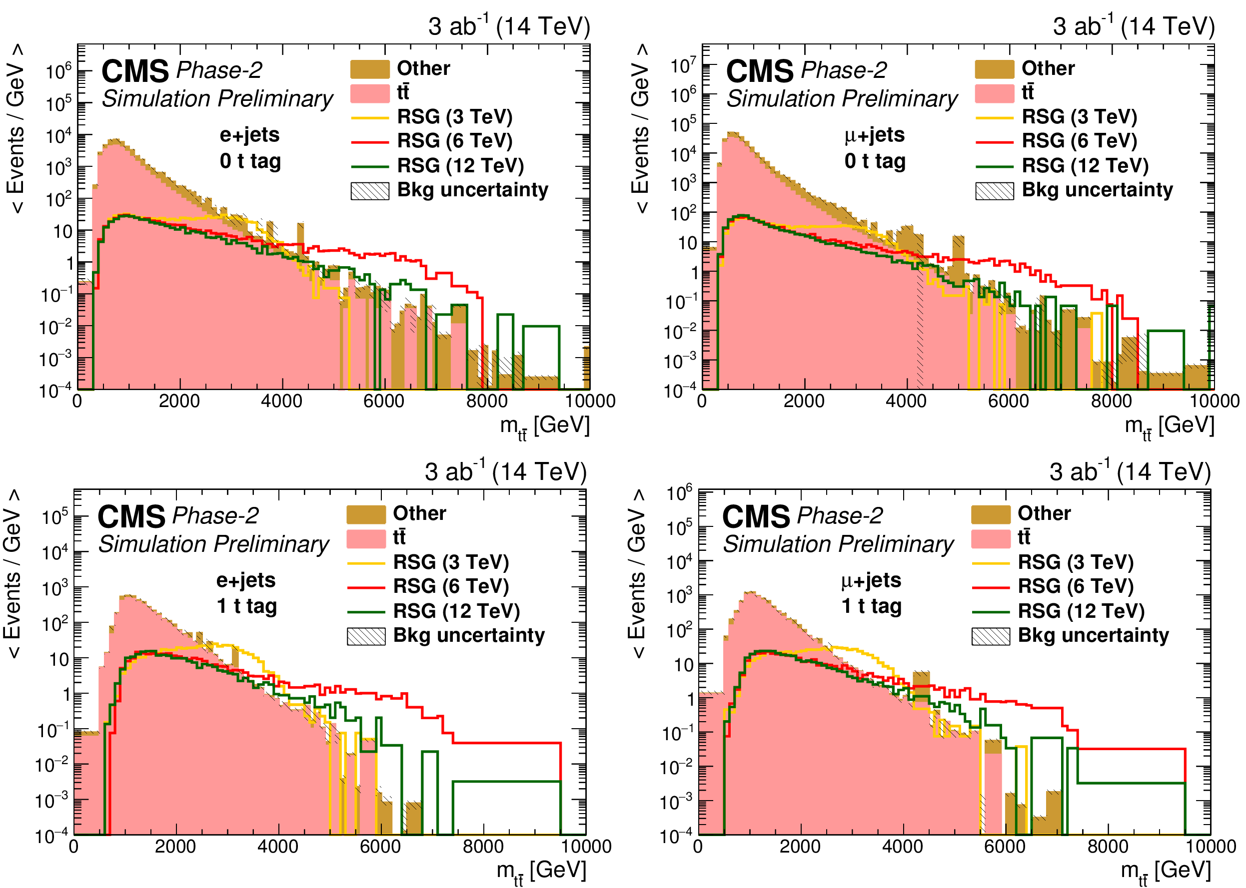
Figure 3:
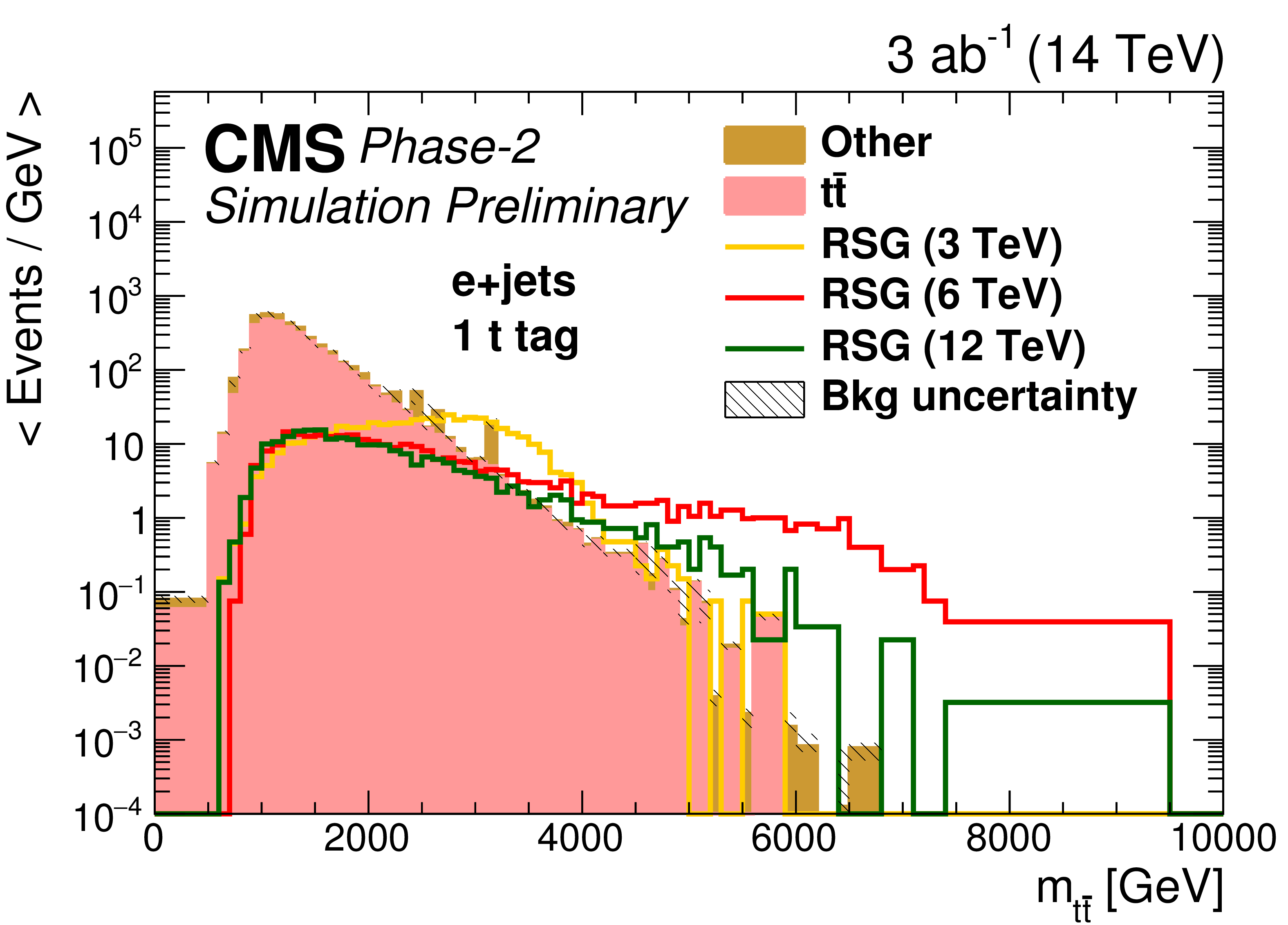
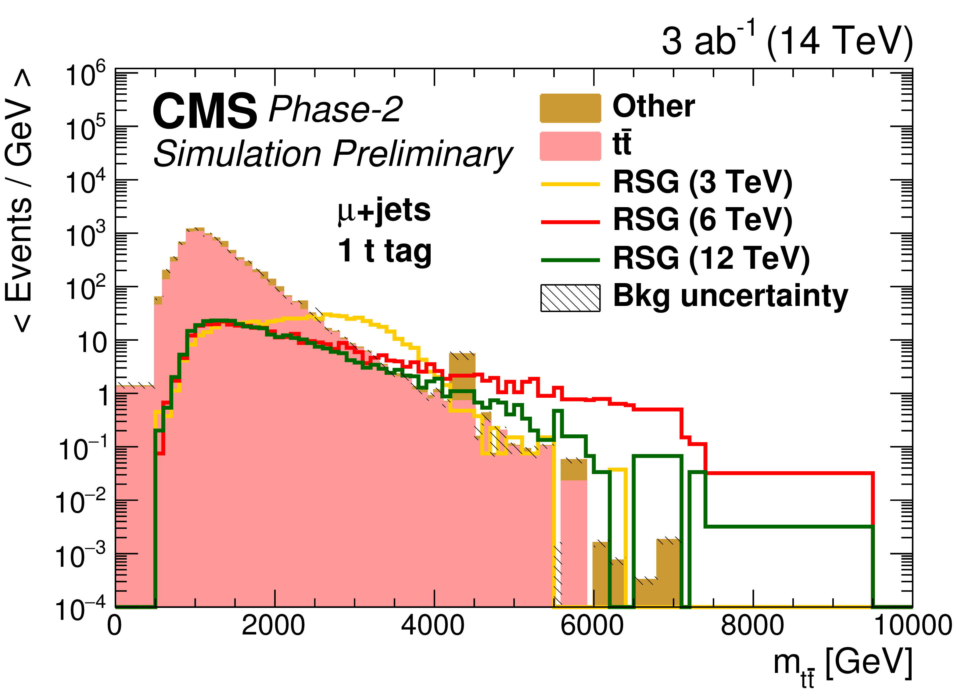
The distributions of $m_{{{\mathrm {t}\overline {\mathrm {t}}}}}$ in events with (top) zero or (bottom) one $ {\mathrm {t}}$-tagged jets for (left) single-electron or (right) single-muon samples. The statistical uncertainties are scaled down by the square root of the projected luminosity. Variable sized bins are used for each category so that the statistical uncertainty on the total background in each bin is less than 10%. The bin contents of the distributions are divided by their bin width. The overflow events are added to the last bin and its content is also divided by the width of the last bin. |
png pdf |
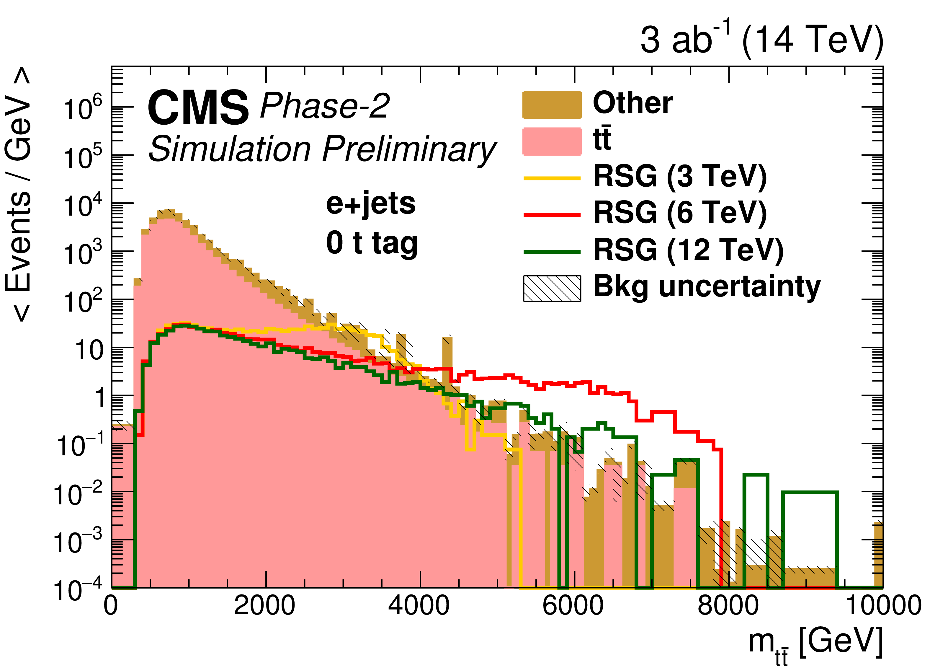
Figure 3-a:
The distributions of $m_{{{\mathrm {t}\overline {\mathrm {t}}}}}$ in events with (top) zero or (bottom) one $ {\mathrm {t}}$-tagged jets for (left) single-electron or (right) single-muon samples. The statistical uncertainties are scaled down by the square root of the projected luminosity. Variable sized bins are used for each category so that the statistical uncertainty on the total background in each bin is less than 10%. The bin contents of the distributions are divided by their bin width. The overflow events are added to the last bin and its content is also divided by the width of the last bin. |
png pdf |
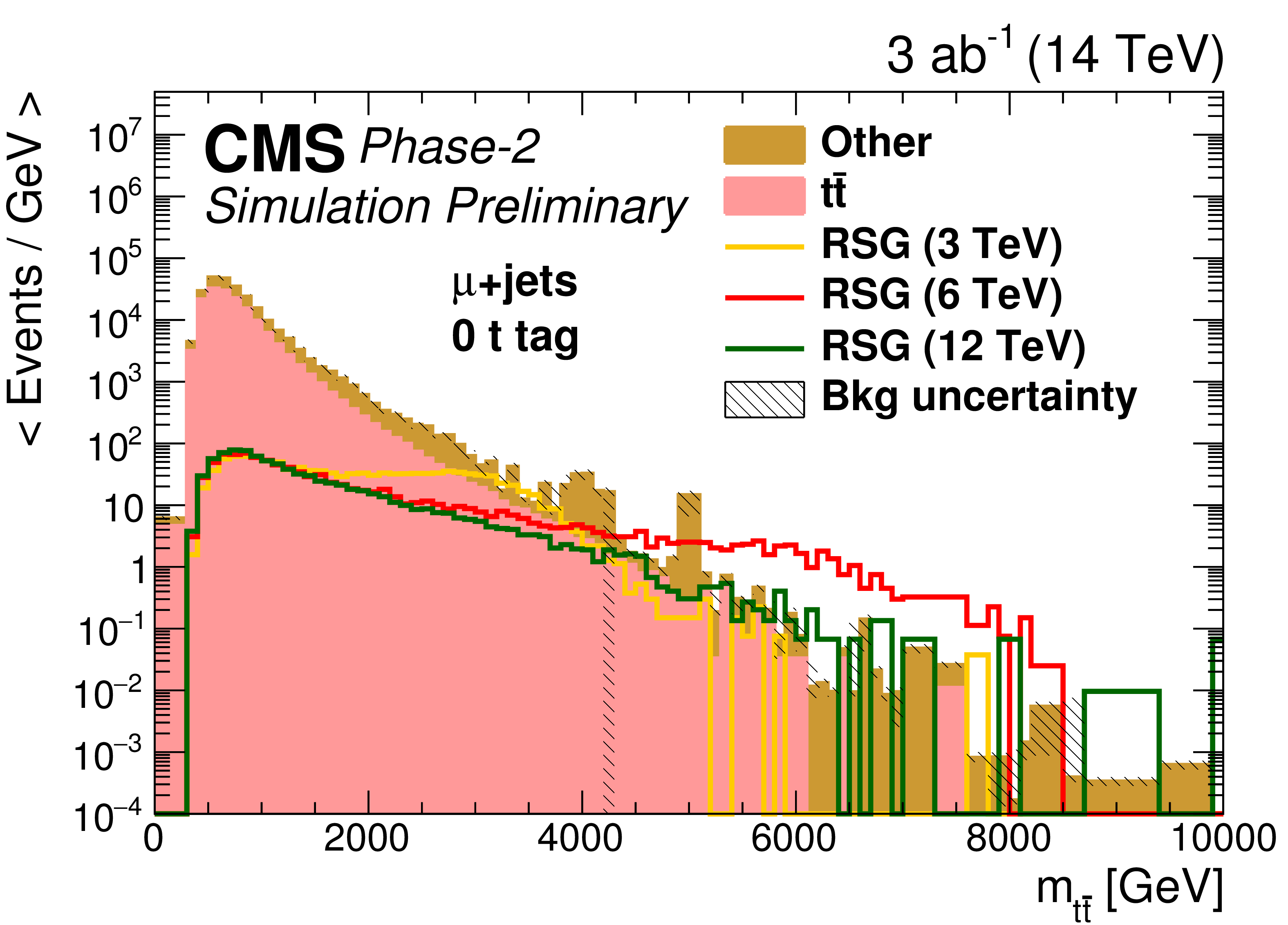
Figure 3-b:
The distributions of $m_{{{\mathrm {t}\overline {\mathrm {t}}}}}$ in events with (top) zero or (bottom) one $ {\mathrm {t}}$-tagged jets for (left) single-electron or (right) single-muon samples. The statistical uncertainties are scaled down by the square root of the projected luminosity. Variable sized bins are used for each category so that the statistical uncertainty on the total background in each bin is less than 10%. The bin contents of the distributions are divided by their bin width. The overflow events are added to the last bin and its content is also divided by the width of the last bin. |
png pdf |
Figure 3-c:
The distributions of $m_{{{\mathrm {t}\overline {\mathrm {t}}}}}$ in events with (top) zero or (bottom) one $ {\mathrm {t}}$-tagged jets for (left) single-electron or (right) single-muon samples. The statistical uncertainties are scaled down by the square root of the projected luminosity. Variable sized bins are used for each category so that the statistical uncertainty on the total background in each bin is less than 10%. The bin contents of the distributions are divided by their bin width. The overflow events are added to the last bin and its content is also divided by the width of the last bin. |
png pdf |
Figure 3-d:
The distributions of $m_{{{\mathrm {t}\overline {\mathrm {t}}}}}$ in events with (top) zero or (bottom) one $ {\mathrm {t}}$-tagged jets for (left) single-electron or (right) single-muon samples. The statistical uncertainties are scaled down by the square root of the projected luminosity. Variable sized bins are used for each category so that the statistical uncertainty on the total background in each bin is less than 10%. The bin contents of the distributions are divided by their bin width. The overflow events are added to the last bin and its content is also divided by the width of the last bin. |

png pdf |
Figure 4:
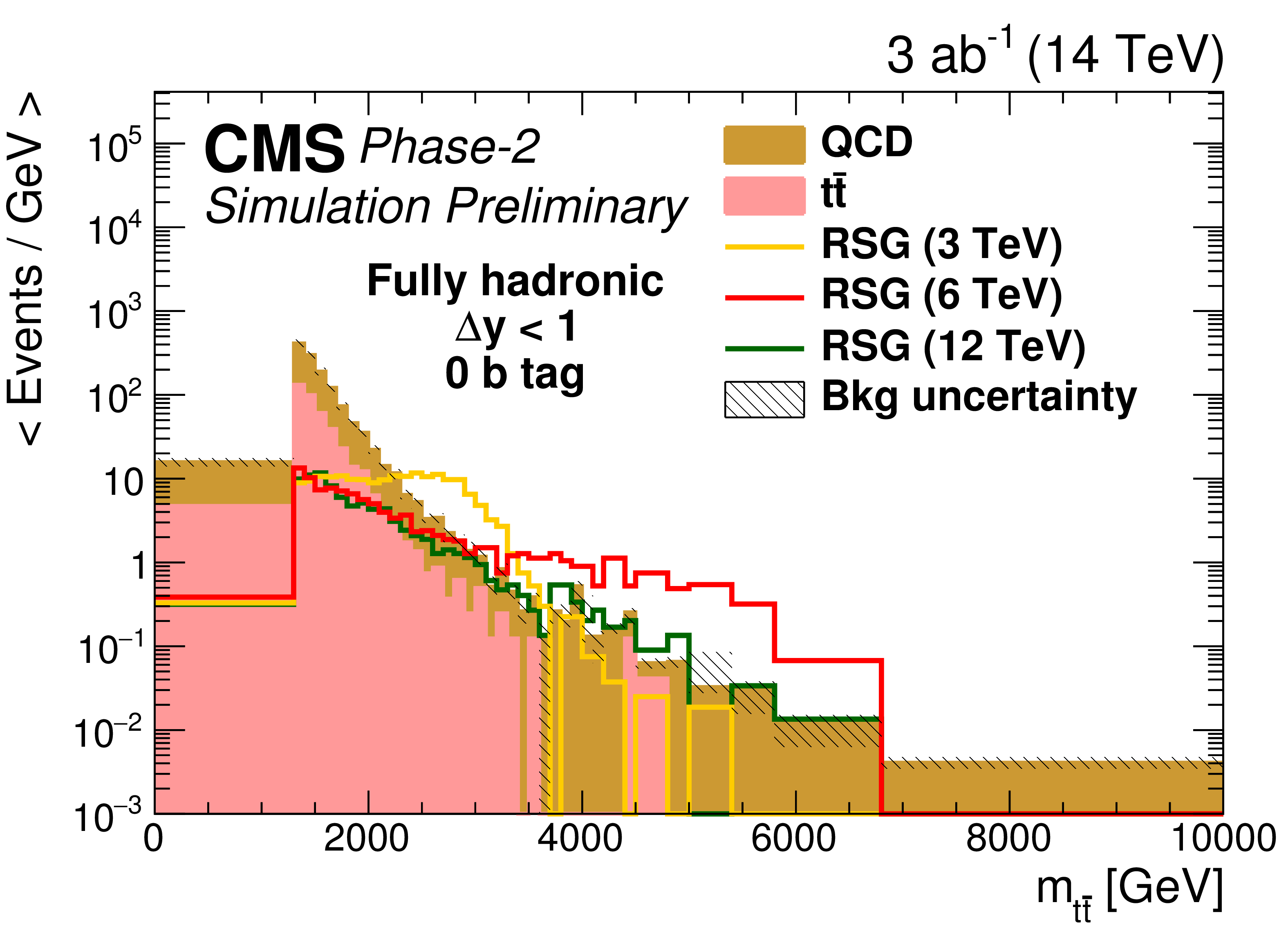
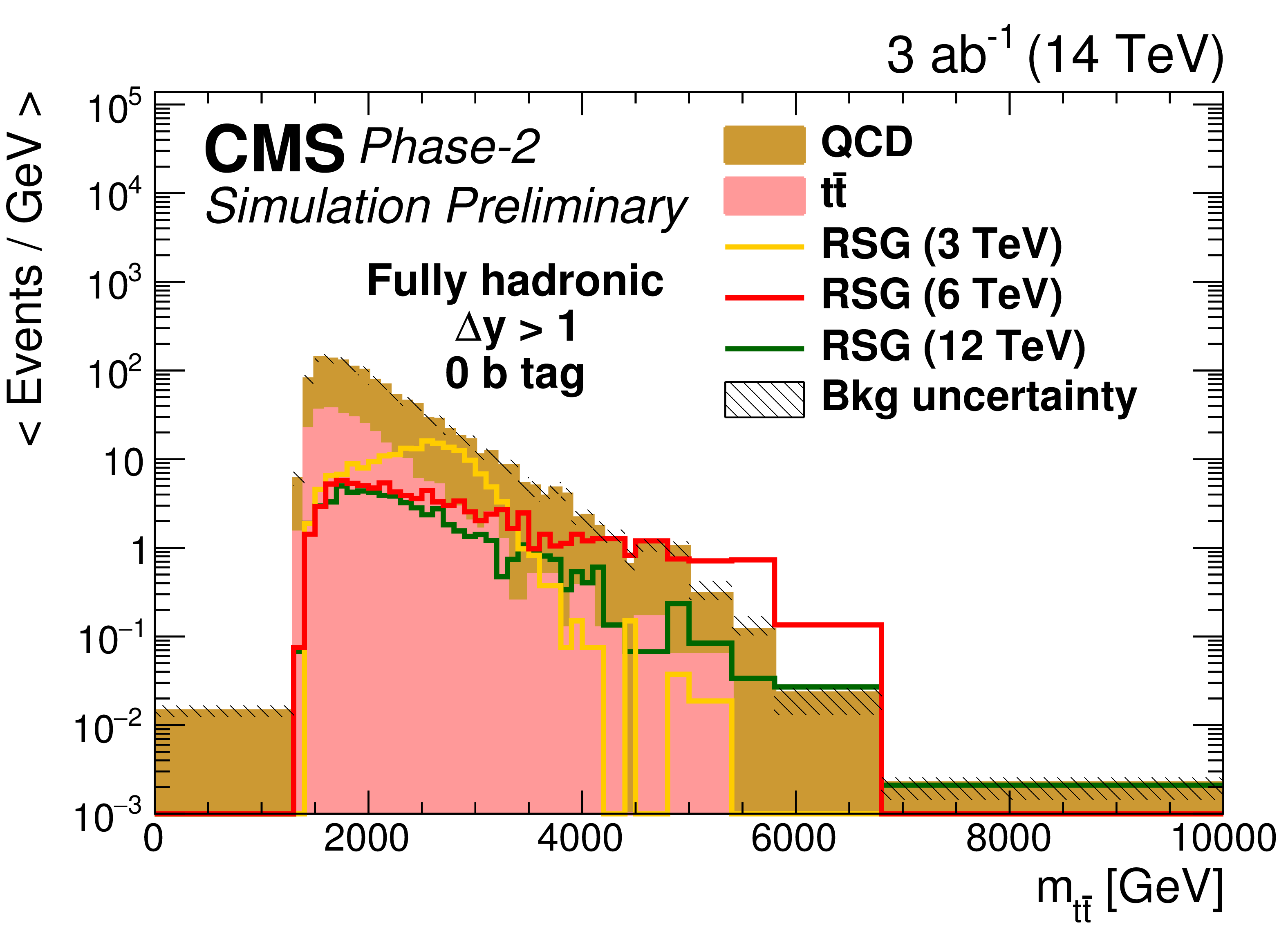
The distribution of the RSG candidate mass for (left) ${\Delta y < 1}$ or (right) ${\Delta y > 1}$ in the (top) zero, (middle) one, or (bottom) two $ {\mathrm {b}}$-tag event categories in the fully hadronic final state. All variables presented after full selection. Along with the RSG signal, the two main backgrounds are shown: ${{\mathrm {t}\overline {\mathrm {t}}}}$ and QCD multijets. The statistical uncertainties are scaled down by the square root of the projected luminosity. Variable sized bins are used for each category so that the statistical uncertainty on the total background in each bin is less than 10%. The bin contents of the distributions are divided by their bin width. The overflow events are added to the last bin and its content is also divided by the width of the last bin. |
png pdf |
Figure 4-a:
The distribution of the RSG candidate mass for (left) ${\Delta y < 1}$ or (right) ${\Delta y > 1}$ in the (top) zero, (middle) one, or (bottom) two $ {\mathrm {b}}$-tag event categories in the fully hadronic final state. All variables presented after full selection. Along with the RSG signal, the two main backgrounds are shown: ${{\mathrm {t}\overline {\mathrm {t}}}}$ and QCD multijets. The statistical uncertainties are scaled down by the square root of the projected luminosity. Variable sized bins are used for each category so that the statistical uncertainty on the total background in each bin is less than 10%. The bin contents of the distributions are divided by their bin width. The overflow events are added to the last bin and its content is also divided by the width of the last bin. |
png pdf |
Figure 4-b:
The distribution of the RSG candidate mass for (left) ${\Delta y < 1}$ or (right) ${\Delta y > 1}$ in the (top) zero, (middle) one, or (bottom) two $ {\mathrm {b}}$-tag event categories in the fully hadronic final state. All variables presented after full selection. Along with the RSG signal, the two main backgrounds are shown: ${{\mathrm {t}\overline {\mathrm {t}}}}$ and QCD multijets. The statistical uncertainties are scaled down by the square root of the projected luminosity. Variable sized bins are used for each category so that the statistical uncertainty on the total background in each bin is less than 10%. The bin contents of the distributions are divided by their bin width. The overflow events are added to the last bin and its content is also divided by the width of the last bin. |

png pdf |
Figure 4-c:
The distribution of the RSG candidate mass for (left) ${\Delta y < 1}$ or (right) ${\Delta y > 1}$ in the (top) zero, (middle) one, or (bottom) two $ {\mathrm {b}}$-tag event categories in the fully hadronic final state. All variables presented after full selection. Along with the RSG signal, the two main backgrounds are shown: ${{\mathrm {t}\overline {\mathrm {t}}}}$ and QCD multijets. The statistical uncertainties are scaled down by the square root of the projected luminosity. Variable sized bins are used for each category so that the statistical uncertainty on the total background in each bin is less than 10%. The bin contents of the distributions are divided by their bin width. The overflow events are added to the last bin and its content is also divided by the width of the last bin. |

png pdf |
Figure 4-d:
The distribution of the RSG candidate mass for (left) ${\Delta y < 1}$ or (right) ${\Delta y > 1}$ in the (top) zero, (middle) one, or (bottom) two $ {\mathrm {b}}$-tag event categories in the fully hadronic final state. All variables presented after full selection. Along with the RSG signal, the two main backgrounds are shown: ${{\mathrm {t}\overline {\mathrm {t}}}}$ and QCD multijets. The statistical uncertainties are scaled down by the square root of the projected luminosity. Variable sized bins are used for each category so that the statistical uncertainty on the total background in each bin is less than 10%. The bin contents of the distributions are divided by their bin width. The overflow events are added to the last bin and its content is also divided by the width of the last bin. |
png pdf |
Figure 4-e:
The distribution of the RSG candidate mass for (left) ${\Delta y < 1}$ or (right) ${\Delta y > 1}$ in the (top) zero, (middle) one, or (bottom) two $ {\mathrm {b}}$-tag event categories in the fully hadronic final state. All variables presented after full selection. Along with the RSG signal, the two main backgrounds are shown: ${{\mathrm {t}\overline {\mathrm {t}}}}$ and QCD multijets. The statistical uncertainties are scaled down by the square root of the projected luminosity. Variable sized bins are used for each category so that the statistical uncertainty on the total background in each bin is less than 10%. The bin contents of the distributions are divided by their bin width. The overflow events are added to the last bin and its content is also divided by the width of the last bin. |

png pdf |
Figure 4-f:
The distribution of the RSG candidate mass for (left) ${\Delta y < 1}$ or (right) ${\Delta y > 1}$ in the (top) zero, (middle) one, or (bottom) two $ {\mathrm {b}}$-tag event categories in the fully hadronic final state. All variables presented after full selection. Along with the RSG signal, the two main backgrounds are shown: ${{\mathrm {t}\overline {\mathrm {t}}}}$ and QCD multijets. The statistical uncertainties are scaled down by the square root of the projected luminosity. Variable sized bins are used for each category so that the statistical uncertainty on the total background in each bin is less than 10%. The bin contents of the distributions are divided by their bin width. The overflow events are added to the last bin and its content is also divided by the width of the last bin. |
png pdf |
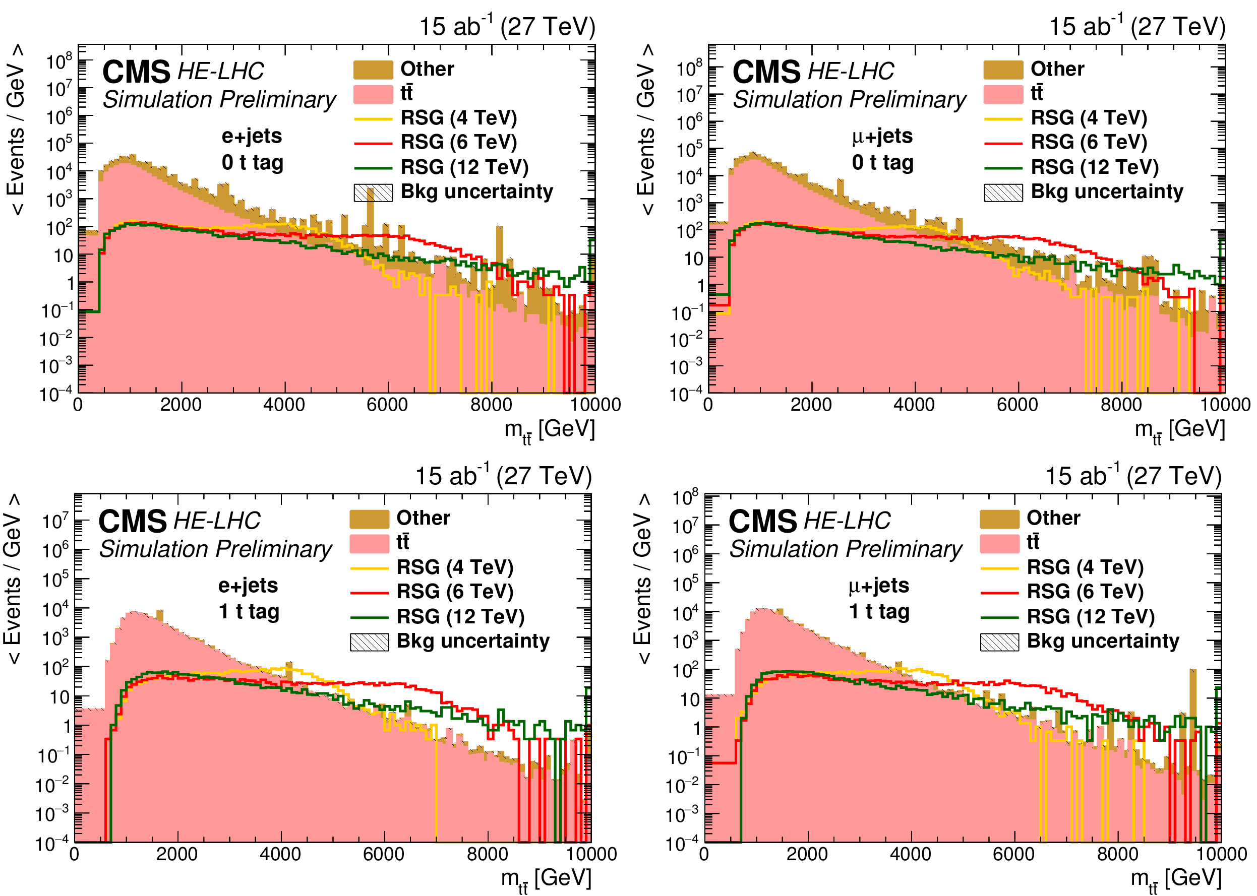
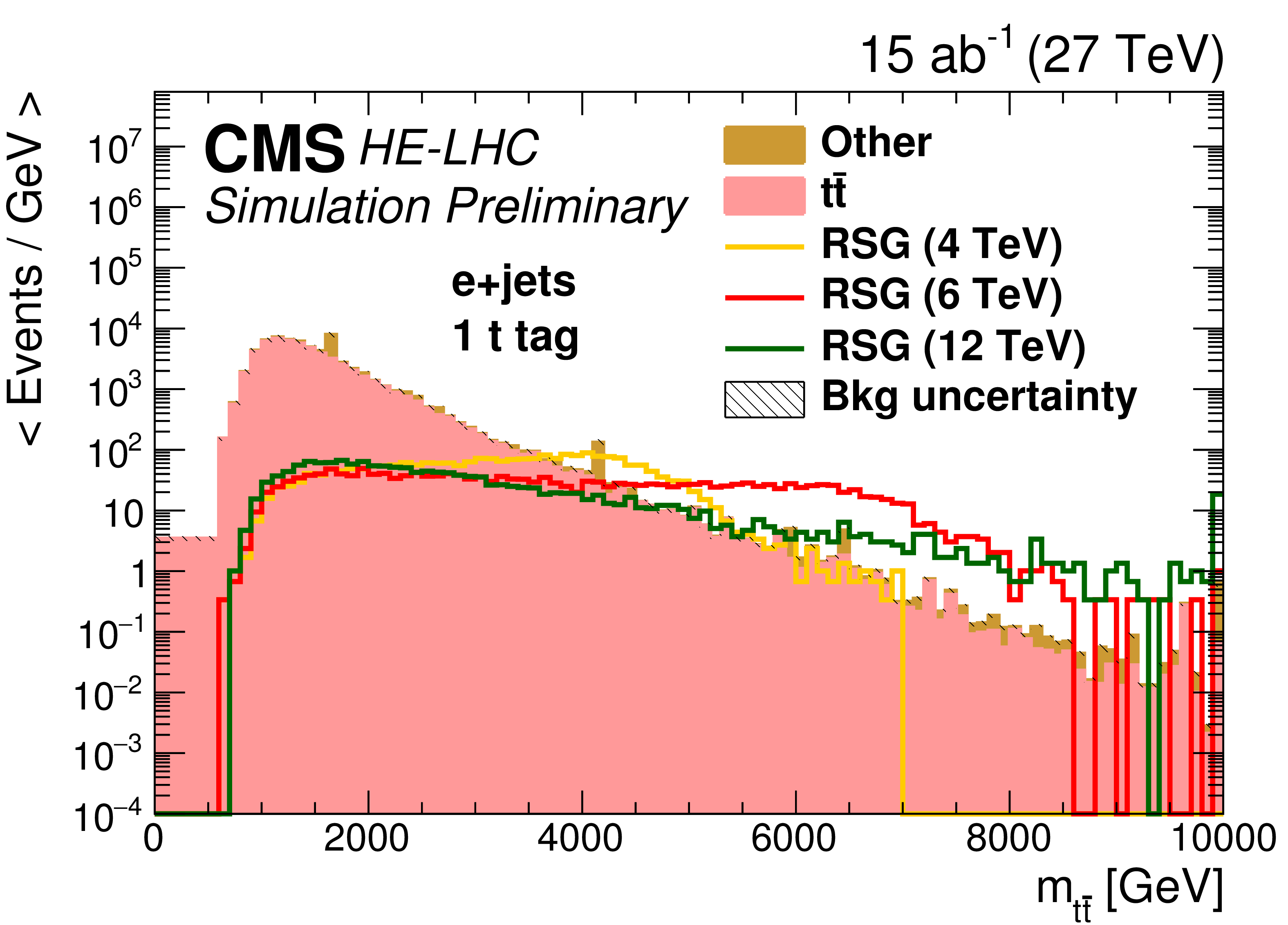
Figure 5:
Distributions of ${m_{{{\mathrm {t}\overline {\mathrm {t}}}}}}$ in events with (top) zero or (bttom) one $ {\mathrm {t}}$-tagged jets for (left) the single-electron or (right) single-muon final state. The statistical uncertainties are scaled down by the square root of the projected luminosity. Variable sized bins are used for each category so that the statistical uncertainty on the total background in each bin is less than 10%. The bin contents of the distributions are divided by their bin width. The overflow events are added to the last bin and its content is also divided by the width of the last bin. |

png pdf |
Figure 5-a:
Distributions of ${m_{{{\mathrm {t}\overline {\mathrm {t}}}}}}$ in events with (top) zero or (bttom) one $ {\mathrm {t}}$-tagged jets for (left) the single-electron or (right) single-muon final state. The statistical uncertainties are scaled down by the square root of the projected luminosity. Variable sized bins are used for each category so that the statistical uncertainty on the total background in each bin is less than 10%. The bin contents of the distributions are divided by their bin width. The overflow events are added to the last bin and its content is also divided by the width of the last bin. |

png pdf |
Figure 5-b:
Distributions of ${m_{{{\mathrm {t}\overline {\mathrm {t}}}}}}$ in events with (top) zero or (bttom) one $ {\mathrm {t}}$-tagged jets for (left) the single-electron or (right) single-muon final state. The statistical uncertainties are scaled down by the square root of the projected luminosity. Variable sized bins are used for each category so that the statistical uncertainty on the total background in each bin is less than 10%. The bin contents of the distributions are divided by their bin width. The overflow events are added to the last bin and its content is also divided by the width of the last bin. |
png pdf |
Figure 5-c:
Distributions of ${m_{{{\mathrm {t}\overline {\mathrm {t}}}}}}$ in events with (top) zero or (bttom) one $ {\mathrm {t}}$-tagged jets for (left) the single-electron or (right) single-muon final state. The statistical uncertainties are scaled down by the square root of the projected luminosity. Variable sized bins are used for each category so that the statistical uncertainty on the total background in each bin is less than 10%. The bin contents of the distributions are divided by their bin width. The overflow events are added to the last bin and its content is also divided by the width of the last bin. |

png pdf |
Figure 5-d:
Distributions of ${m_{{{\mathrm {t}\overline {\mathrm {t}}}}}}$ in events with (top) zero or (bttom) one $ {\mathrm {t}}$-tagged jets for (left) the single-electron or (right) single-muon final state. The statistical uncertainties are scaled down by the square root of the projected luminosity. Variable sized bins are used for each category so that the statistical uncertainty on the total background in each bin is less than 10%. The bin contents of the distributions are divided by their bin width. The overflow events are added to the last bin and its content is also divided by the width of the last bin. |

png pdf |
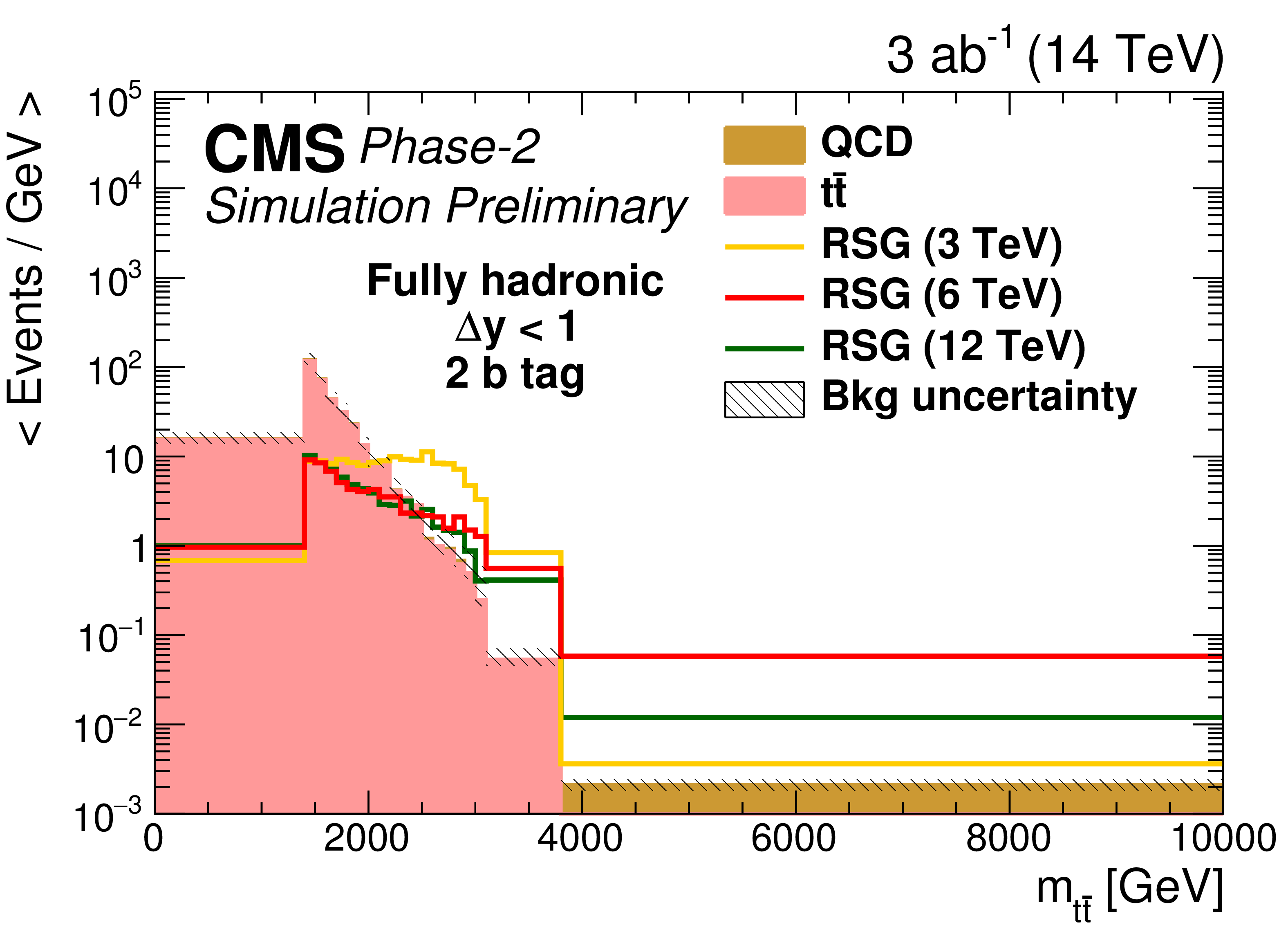
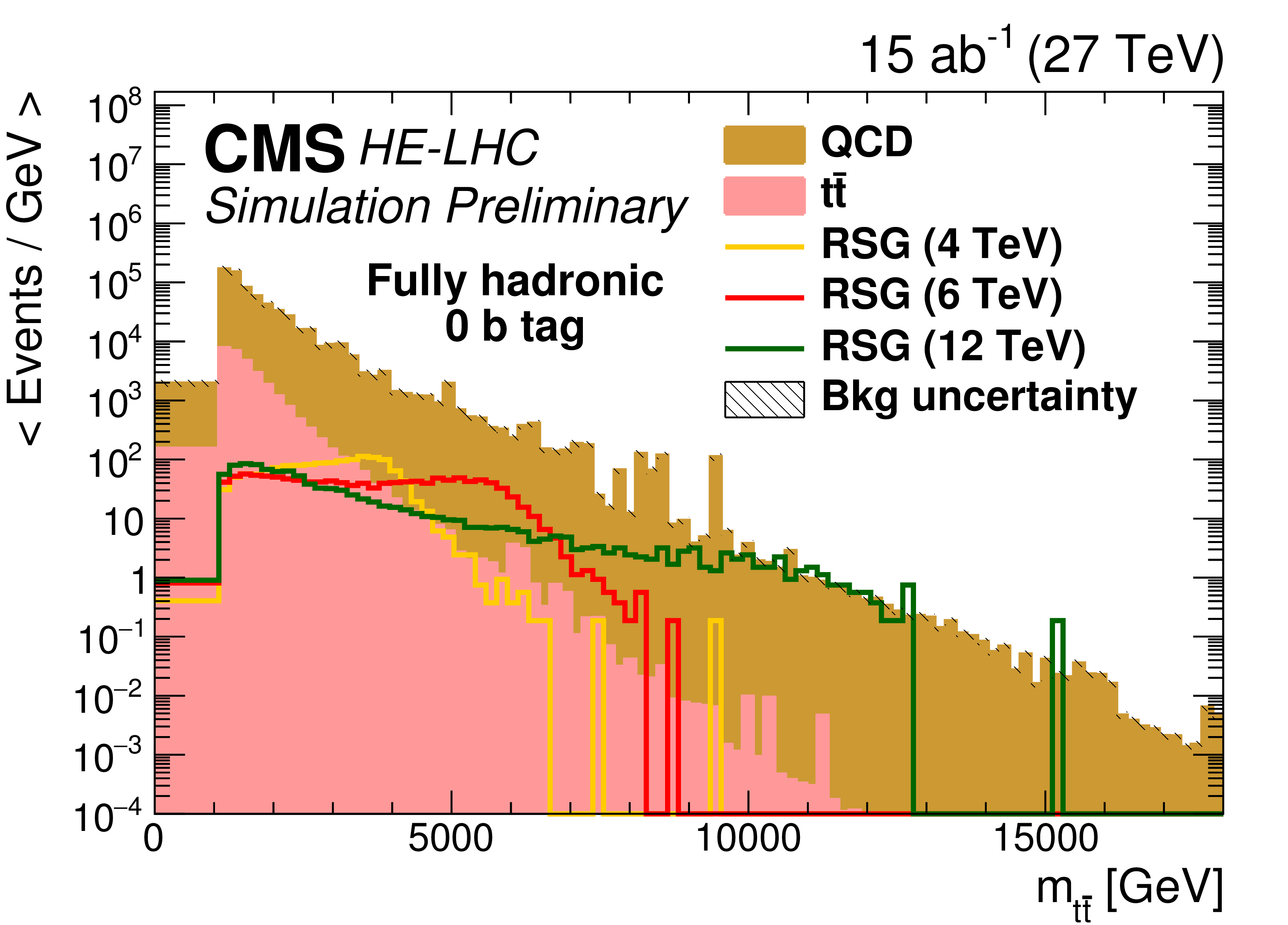
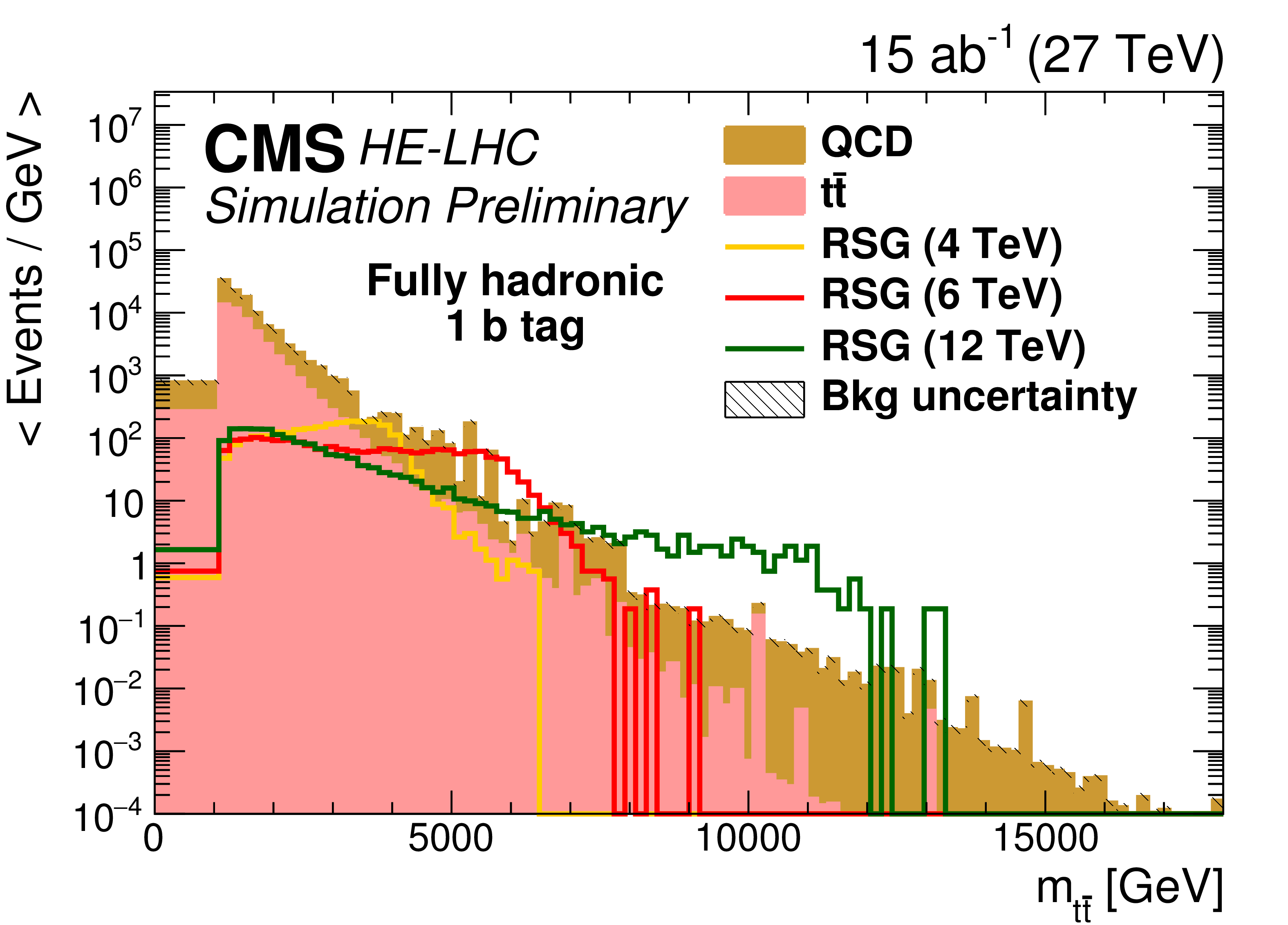
Figure 6:
Distributions of ${m_{{{\mathrm {t}\overline {\mathrm {t}}}}}}$ for (top left) zero, (top right) one, or (bottom) two $ {\mathrm {b}}$ tag event categories in the fully hadronic final state. The statistical uncertainties are scaled down by the square root of the projected luminosity. Variable sized bins are used for each category so that the statistical uncertainty on the total background in each bin is less than 10%. The bin contents of the distributions are divided by their bin width. The overflow events are added to the last bin and its content is also divided by the width of the last bin. |
png pdf |
Figure 6-a:
Distributions of ${m_{{{\mathrm {t}\overline {\mathrm {t}}}}}}$ for (top left) zero, (top right) one, or (bottom) two $ {\mathrm {b}}$ tag event categories in the fully hadronic final state. The statistical uncertainties are scaled down by the square root of the projected luminosity. Variable sized bins are used for each category so that the statistical uncertainty on the total background in each bin is less than 10%. The bin contents of the distributions are divided by their bin width. The overflow events are added to the last bin and its content is also divided by the width of the last bin. |
png pdf |
Figure 6-b:
Distributions of ${m_{{{\mathrm {t}\overline {\mathrm {t}}}}}}$ for (top left) zero, (top right) one, or (bottom) two $ {\mathrm {b}}$ tag event categories in the fully hadronic final state. The statistical uncertainties are scaled down by the square root of the projected luminosity. Variable sized bins are used for each category so that the statistical uncertainty on the total background in each bin is less than 10%. The bin contents of the distributions are divided by their bin width. The overflow events are added to the last bin and its content is also divided by the width of the last bin. |

png pdf |
Figure 6-c:
Distributions of ${m_{{{\mathrm {t}\overline {\mathrm {t}}}}}}$ for (top left) zero, (top right) one, or (bottom) two $ {\mathrm {b}}$ tag event categories in the fully hadronic final state. The statistical uncertainties are scaled down by the square root of the projected luminosity. Variable sized bins are used for each category so that the statistical uncertainty on the total background in each bin is less than 10%. The bin contents of the distributions are divided by their bin width. The overflow events are added to the last bin and its content is also divided by the width of the last bin. |
png pdf |
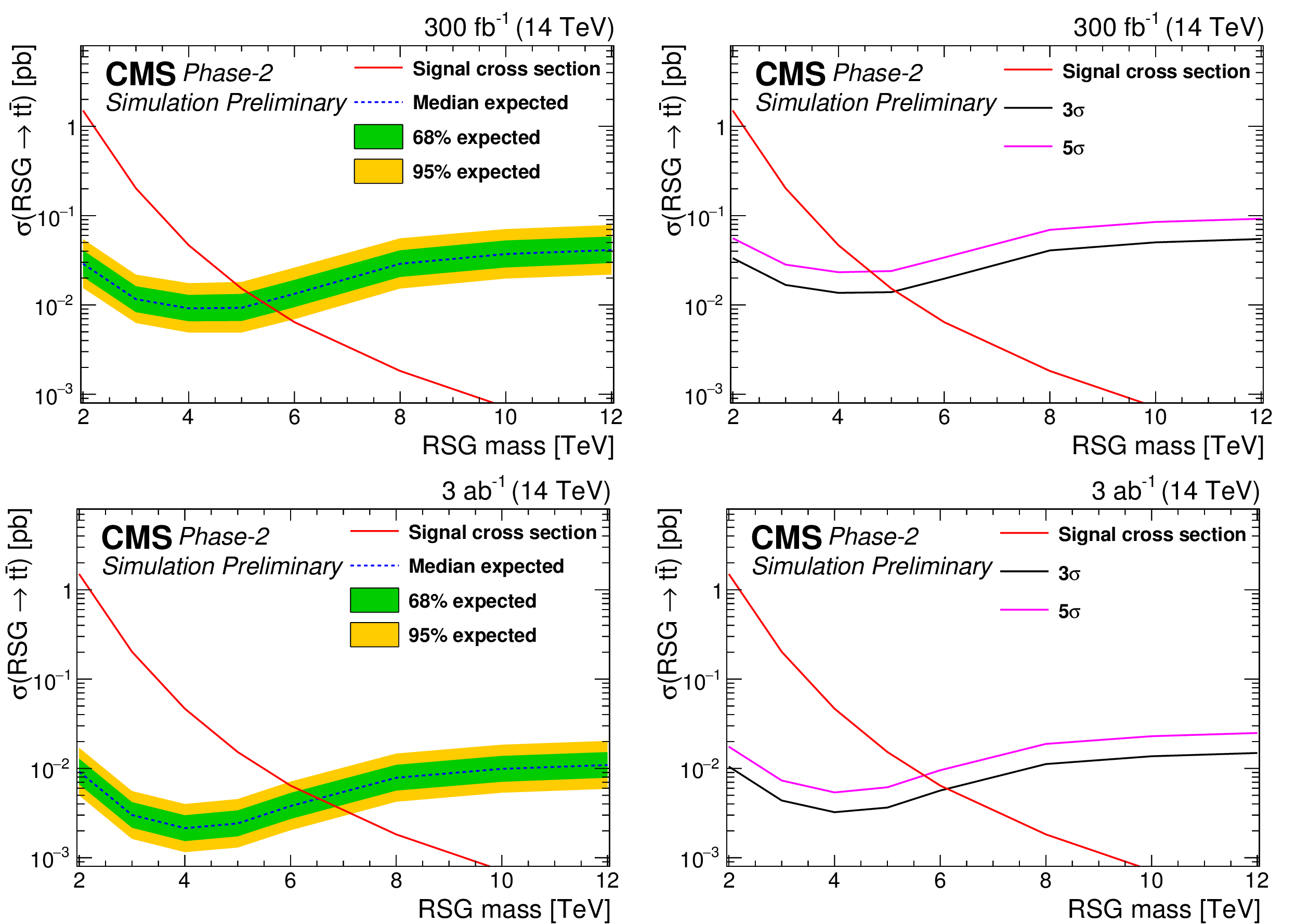
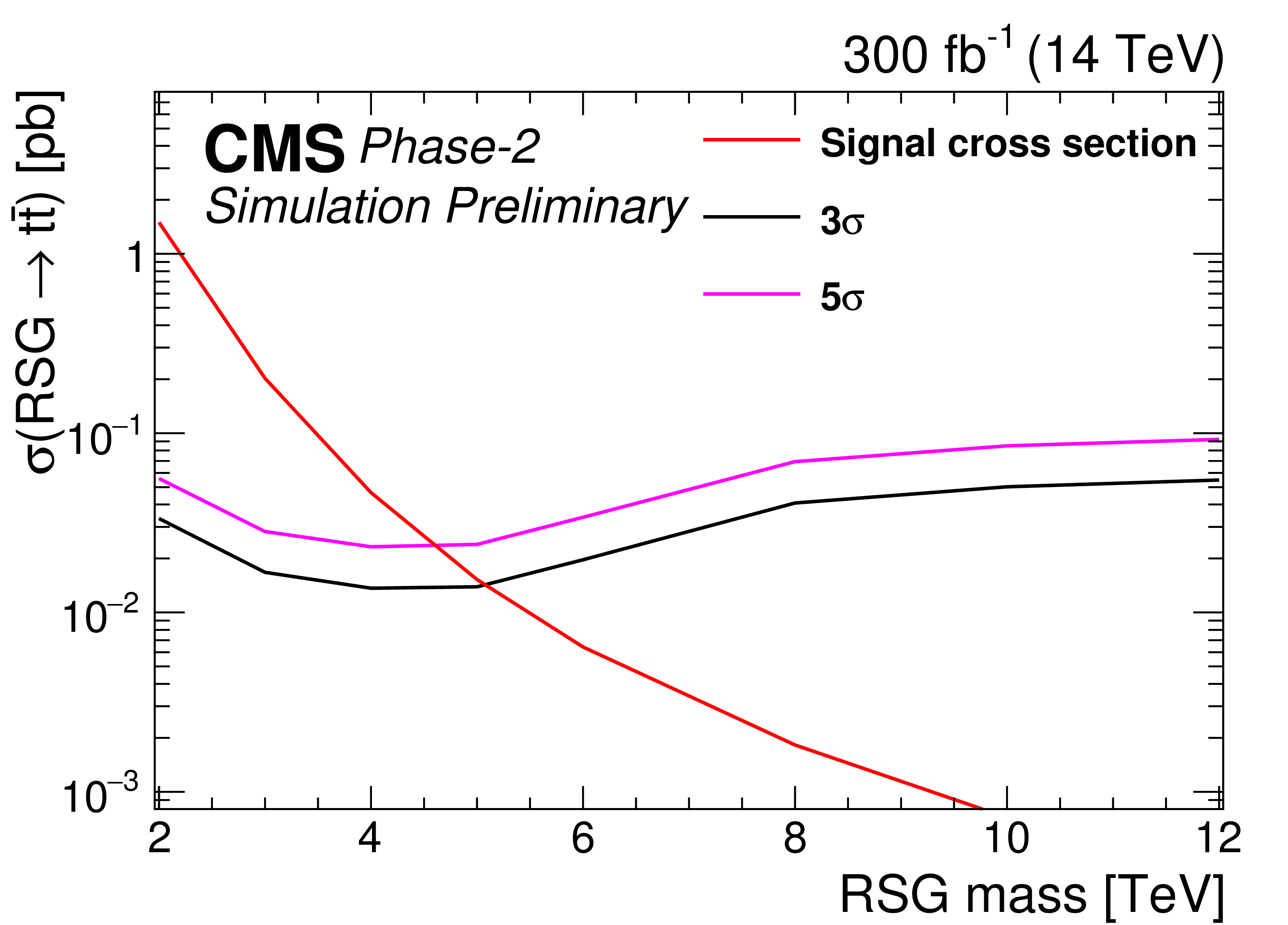
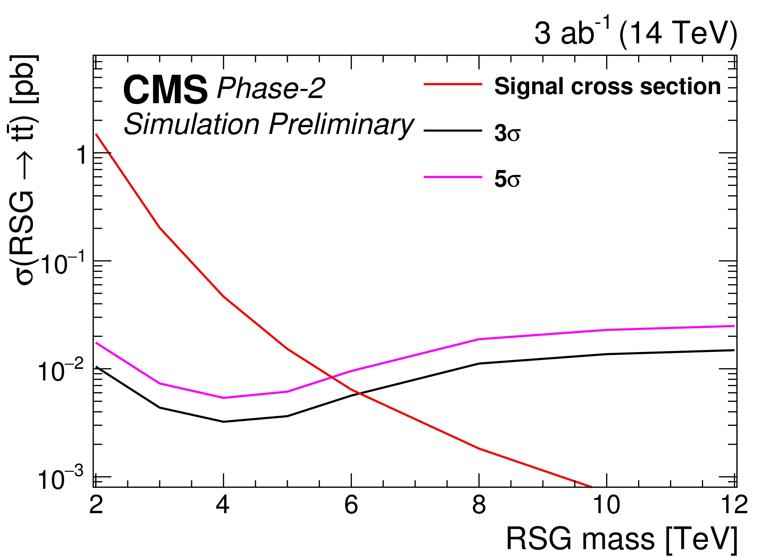
Figure 7:
95% CL expected upper limits (left) and 3$\sigma $ and 5$\sigma $ discovery reaches (right) for an RSG decaying to ${{\mathrm {t}\overline {\mathrm {t}}}}$ at 300 fb$^{-1}$ (top) and 3 ab$^{-1}$ (bottom) for the combined single-lepton and fully hadronic final states. The LO signal theory cross sections are scaled to NLO using a $k$ factor of 1.3 [44]. |

png pdf |
Figure 7-a:
95% CL expected upper limits (left) and 3$\sigma $ and 5$\sigma $ discovery reaches (right) for an RSG decaying to ${{\mathrm {t}\overline {\mathrm {t}}}}$ at 300 fb$^{-1}$ (top) and 3 ab$^{-1}$ (bottom) for the combined single-lepton and fully hadronic final states. The LO signal theory cross sections are scaled to NLO using a $k$ factor of 1.3 [44]. |
png pdf |
Figure 7-b:
95% CL expected upper limits (left) and 3$\sigma $ and 5$\sigma $ discovery reaches (right) for an RSG decaying to ${{\mathrm {t}\overline {\mathrm {t}}}}$ at 300 fb$^{-1}$ (top) and 3 ab$^{-1}$ (bottom) for the combined single-lepton and fully hadronic final states. The LO signal theory cross sections are scaled to NLO using a $k$ factor of 1.3 [44]. |

png pdf |
Figure 7-c:
95% CL expected upper limits (left) and 3$\sigma $ and 5$\sigma $ discovery reaches (right) for an RSG decaying to ${{\mathrm {t}\overline {\mathrm {t}}}}$ at 300 fb$^{-1}$ (top) and 3 ab$^{-1}$ (bottom) for the combined single-lepton and fully hadronic final states. The LO signal theory cross sections are scaled to NLO using a $k$ factor of 1.3 [44]. |
png pdf |
Figure 7-d:
95% CL expected upper limits (left) and 3$\sigma $ and 5$\sigma $ discovery reaches (right) for an RSG decaying to ${{\mathrm {t}\overline {\mathrm {t}}}}$ at 300 fb$^{-1}$ (top) and 3 ab$^{-1}$ (bottom) for the combined single-lepton and fully hadronic final states. The LO signal theory cross sections are scaled to NLO using a $k$ factor of 1.3 [44]. |
png pdf |
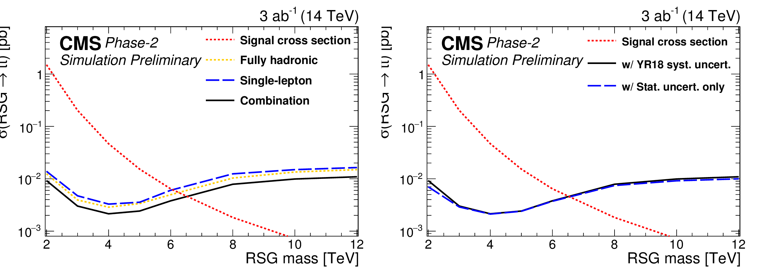
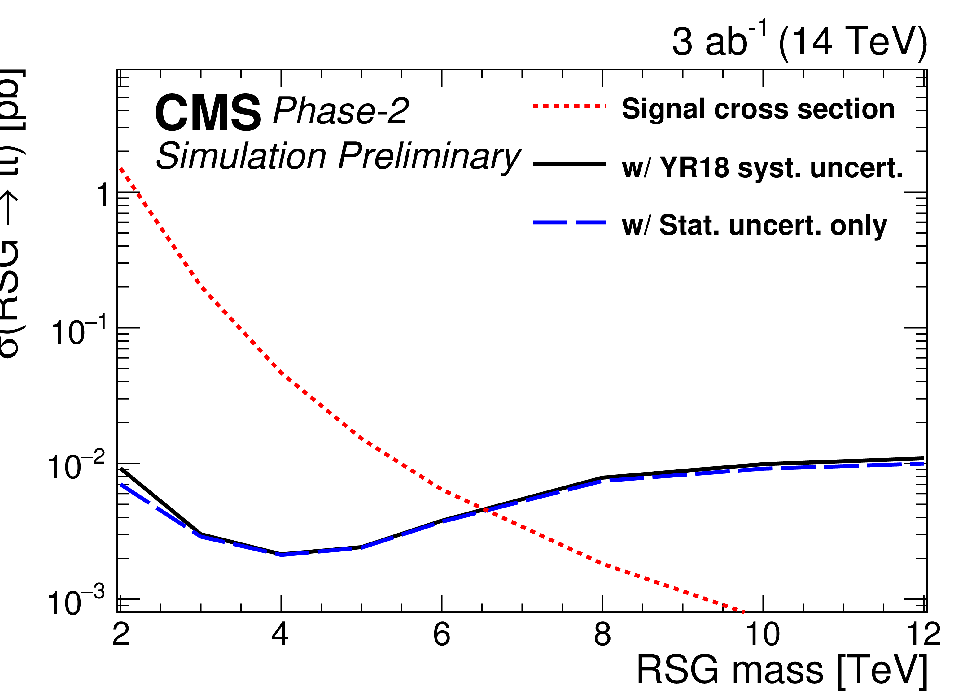
Figure 8:
95% CL expected cross section limits for 3 ab$^{-1}$ projection. Comparisons of the contributions from each final state to the combination is shown on the left. The effect of different systematic uncertainty scenarios on the combined limits is shown on the right. The LO signal theory cross sections are scaled to NLO using a $k$ factor of 1.3 [44]. |

png pdf |
Figure 8-a:
95% CL expected cross section limits for 3 ab$^{-1}$ projection. Comparisons of the contributions from each final state to the combination is shown on the left. The effect of different systematic uncertainty scenarios on the combined limits is shown on the right. The LO signal theory cross sections are scaled to NLO using a $k$ factor of 1.3 [44]. |
png pdf |
Figure 8-b:
95% CL expected cross section limits for 3 ab$^{-1}$ projection. Comparisons of the contributions from each final state to the combination is shown on the left. The effect of different systematic uncertainty scenarios on the combined limits is shown on the right. The LO signal theory cross sections are scaled to NLO using a $k$ factor of 1.3 [44]. |
png pdf |
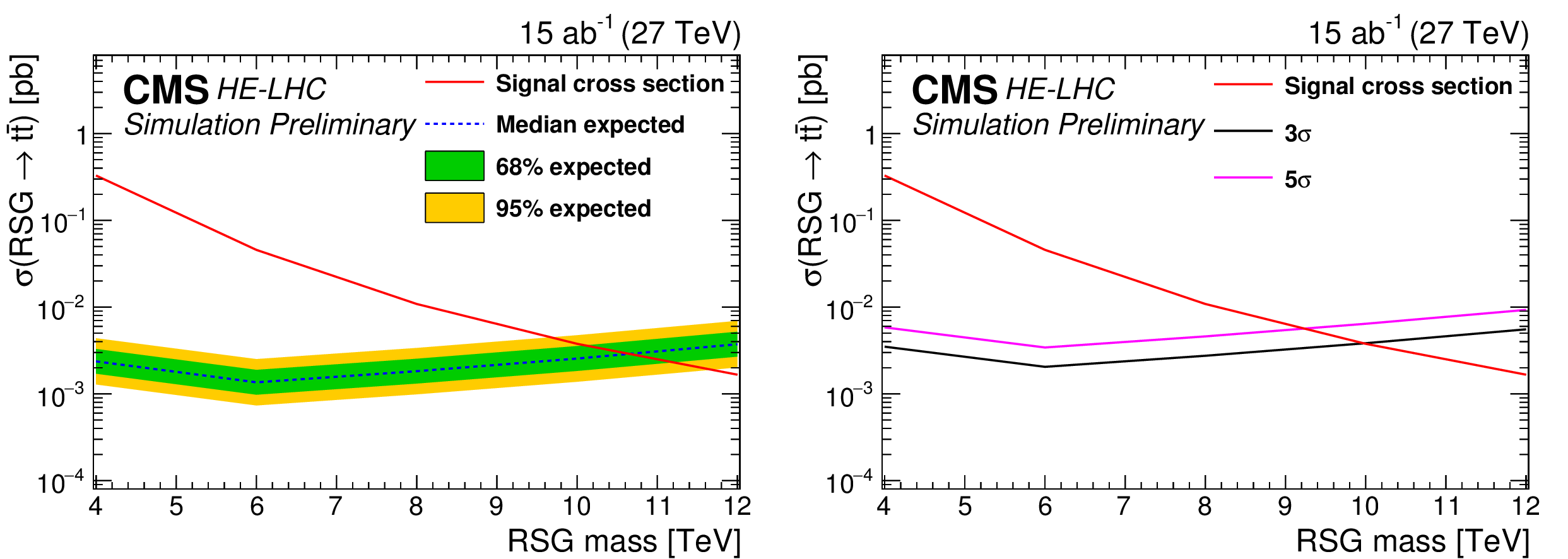
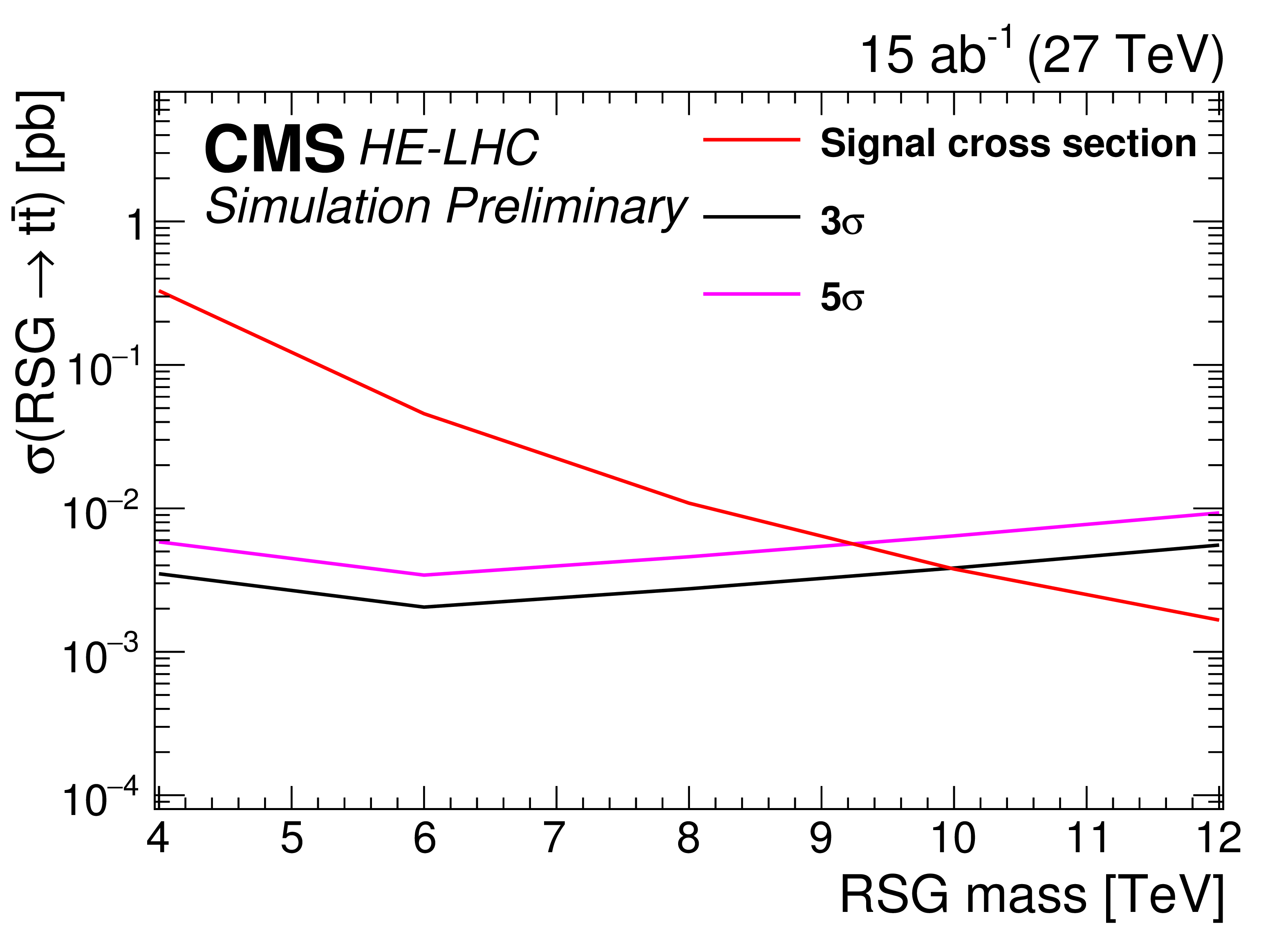
Figure 9:
95% CL expected upper limits (left) and 3$\sigma $ and 5$\sigma $ discovery potential (right) for an RSG decaying to $ {{\mathrm {t}\overline {\mathrm {t}}}} $ with 15 ab$^{-1}$ from the HE-LHC for the combined single-lepton and fully hadronic final states. The LO signal theory cross sections are scaled to NLO using a $k$ factor of 1.3 [44]. |

png pdf |
Figure 9-a:
95% CL expected upper limits (left) and 3$\sigma $ and 5$\sigma $ discovery potential (right) for an RSG decaying to $ {{\mathrm {t}\overline {\mathrm {t}}}} $ with 15 ab$^{-1}$ from the HE-LHC for the combined single-lepton and fully hadronic final states. The LO signal theory cross sections are scaled to NLO using a $k$ factor of 1.3 [44]. |
png pdf |
Figure 9-b:
95% CL expected upper limits (left) and 3$\sigma $ and 5$\sigma $ discovery potential (right) for an RSG decaying to $ {{\mathrm {t}\overline {\mathrm {t}}}} $ with 15 ab$^{-1}$ from the HE-LHC for the combined single-lepton and fully hadronic final states. The LO signal theory cross sections are scaled to NLO using a $k$ factor of 1.3 [44]. |
| Tables | |

png pdf |
Table 1:
Summary of the selection efficiencies for the two final states for the signal hypotheses considered. |

png pdf |
Table 2:
Summary of the sources of systematic uncertainties. |
png pdf |
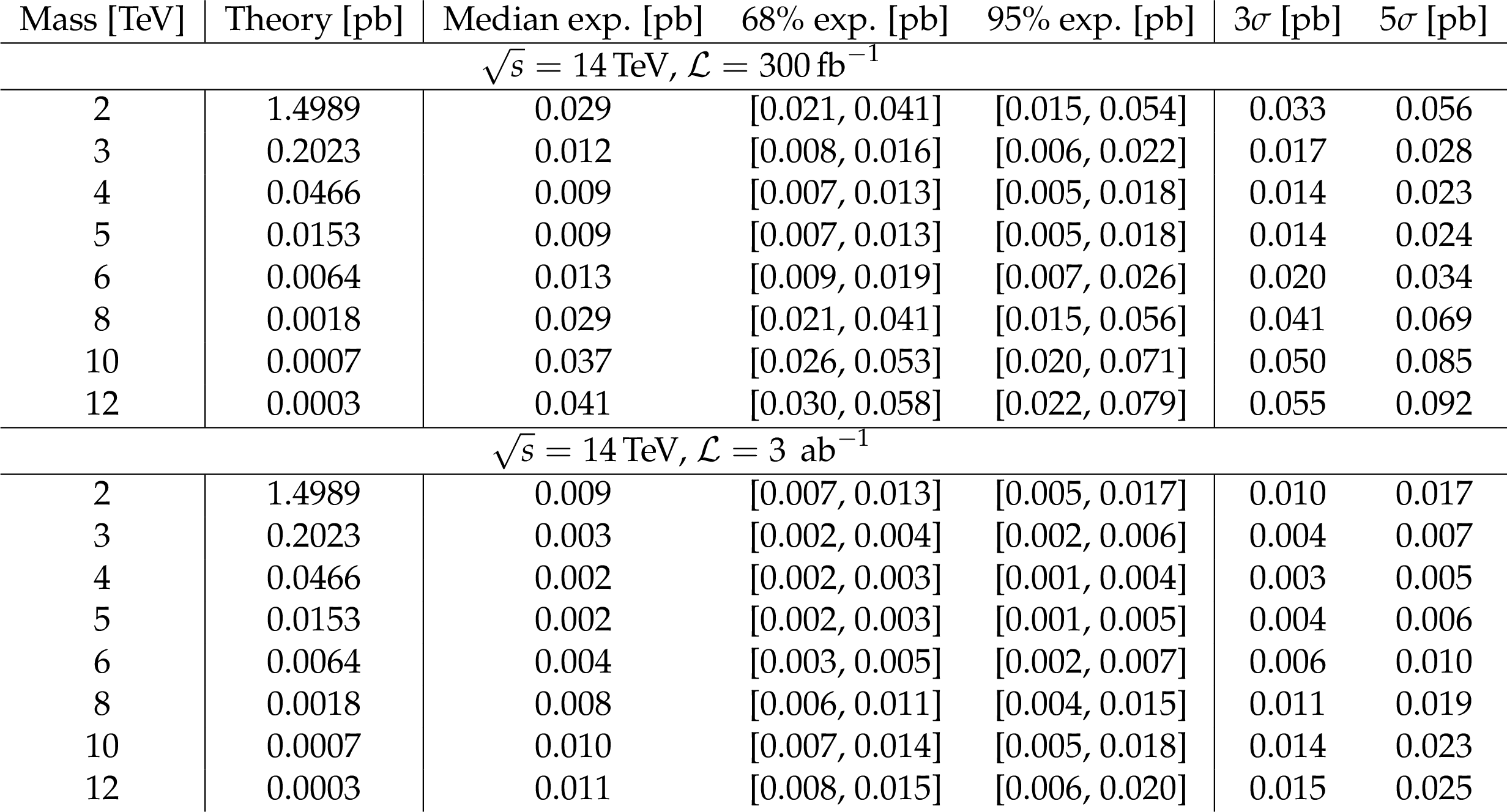
Table 3:
Expected cross section limits at 95% CL and discovery reaches at 3 and 5$\sigma $ in the combined single-lepton and fully hadronic final states for an RSG decaying to $ {{\mathrm {t}\overline {\mathrm {t}}}} $. The LO signal theory cross sections are scaled to NLO using a $k$ factor of 1.3 [44]. |
png pdf |
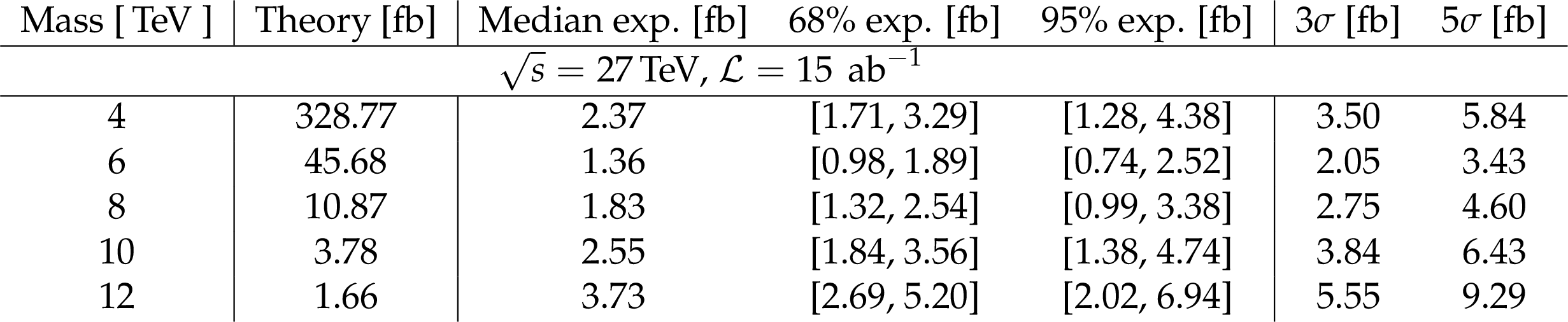
Table 4:
Expected cross section limits at 95% CL and discovery potential at 3$\sigma $ and 5$\sigma $ in the combined single-lepton and fully hadronic final states for an RSG decaying to $ {{\mathrm {t}\overline {\mathrm {t}}}} $ with 15 ab$^{-1}$ from the HE-LHC. The LO signal theory cross sections are scaled to NLO using a $k$ factor of 1.3 [44]. |
| Summary |
| We have presented a sensitivity projection for heavy resonant $\mathrm{t\bar{t}}$ pair production using the upgraded Phase-2 CMS detector design at the High-Luminosity LHC (HL-LHC) and High-Energy LHC (HE-LHC), with center-of-mass energies of 14 and 27 TeV and integrated luminosities of 3 and 15 ab$^{-1}$. Two distinct final states, single-lepton or fully hadronic, are considered. We set limits on the production cross sections of a Randall-Sundrum gluon and exclude masses up to 6.6 (10.7) TeV at 95% confidence level at the HL-LHC (HE-LHC). The Randall-Sundrum gluon with a mass up to 5.7 (9.4) TeV can be discovered with 5$\sigma$ significance at the HL-LHC (HE-LHC). |
| References | ||||
| 1 | S. Dimopoulos and H. Georgi | Softly Broken Supersymmetry and SU(5) | NPB 193 (1981) 150 | |
| 2 | S. Weinberg | Implications of Dynamical Symmetry Breaking | PRD 13 (1976) 974 | |
| 3 | L. Susskind | Dynamics of Spontaneous Symmetry Breaking in the Weinberg- Salam Theory | PRD 20 (1979) 2619 | |
| 4 | C. T. Hill and S. J. Parke | Top production: Sensitivity to new physics | PRD 49 (1994) 4454 | hep-ph/9312324 |
| 5 | R. S. Chivukula, B. A. Dobrescu, H. Georgi, and C. T. Hill | Top quark seesaw theory of electroweak symmetry breaking | PRD 59 (1999) 075003 | hep-ph/9809470 |
| 6 | N. Arkani-Hamed, A. G. Cohen, and H. Georgi | Electroweak symmetry breaking from dimensional deconstruction | PLB 513 (2001) 232 | hep-ph/0105239 |
| 7 | N. Arkani-Hamed, S. Dimopoulos, and G. R. Dvali | The hierarchy problem and new dimensions at a millimeter | PLB 429 (1998) 263 | hep-ph/9803315 |
| 8 | L. Randall and R. Sundrum | A large mass hierarchy from a small extra dimension | PRL 83 (1999) 3370 | hep-ph/9905221 |
| 9 | L. Randall and R. Sundrum | An alternative to compactification | PRL 83 (1999) 4690 | hep-th/9906064 |
| 10 | CMS Collaboration | Search for BSM $ \mathrm{t\bar{t}} $ Production in the Boosted All-Hadronic Final State | CDS | |
| 11 | CMS Collaboration | Search for resonant ttbar production in proton-proton collisions at $ \sqrt{s}= $ 8 TeV | PRD 93 (2016) 012001 | CMS-B2G-13-008 1506.03062 |
| 12 | CMS Collaboration | Search for resonant $ \mathrm{t\bar{t}} $ production in proton-proton collisions at $ \sqrt{s}= $ 13 TeV | Submitted to: JHEP | CMS-B2G-17-017 1810.05905 |
| 13 | CMS Collaboration | The CMS Experiment at the CERN LHC | JINST 3 (2008) S08004 | CMS-00-001 |
| 14 | CMS Collaboration | Technical Proposal for the Phase-II Upgrade of the CMS Detector | CMS-PAS-TDR-15-002 | CMS-PAS-TDR-15-002 |
| 15 | CMS Collaboration | The Phase-2 Upgrade of the CMS Tracker | CDS | |
| 16 | CMS Collaboration | The Phase-2 Upgrade of the CMS Barrel Calorimeters Technical Design Report | CDS | |
| 17 | CMS Collaboration | The Phase-2 Upgrade of the CMS Endcap Calorimeter | CDS | |
| 18 | CMS Collaboration | The Phase-2 Upgrade of the CMS Muon Detectors | CDS | |
| 19 | CMS Collaboration | CMS Phase-2 Object Performance | ||
| 20 | T. Sjostrand et al. | An Introduction to PYTHIA 8.2 | CPC 191 (2015) 159 | 1410.3012 |
| 21 | P. Nason | A New Method for Combining NLO QCD with Shower Monte Carlo Algorithms | JHEP 11 (2004) 040 | hep-ph/0409146 |
| 22 | S. Frixione, P. Nason, and C. Oleari | Matching NLO QCD computations with Parton Shower simulations: the POWHEG method | JHEP 11 (2007) 070 | 0709.2092 |
| 23 | S. Alioli, P. Nason, C. Oleari, and E. Re | A general framework for implementing NLO calculations in shower Monte Carlo programs: the POWHEG BOX | JHEP 06 (2010) 043 | 1002.2581 |
| 24 | S. Frixione, P. Nason, and G. Ridolfi | A positive-weight next-to-leading-order Monte Carlo for heavy flavour hadroproduction | JHEP 09 (2007) 126 | 0707.3088 |
| 25 | J. Alwall et al. | The automated computation of tree-level and next-to-leading order differential cross sections, and their matching to parton shower simulations | JHEP 07 (2014) 079 | 1405.0301 |
| 26 | J. Alwall et al. | Comparative study of various algorithms for the merging of parton showers and matrix elements in hadronic collisions | EPJC 53 (2008) 473 | 0706.2569 |
| 27 | R. Frederix and S. Frixione | Merging meets matching in MC@NLO | JHEP 12 (2012) 061 | 1209.6215 |
| 28 | CMS Collaboration | Event generator tunes obtained from underlying event and multiparton scattering measurements | EPJC 76 (2016) 155 | CMS-GEN-14-001 1512.00815 |
| 29 | P. Skands, S. Carrazza, and J. Rojo | Tuning PYTHIA 8.1: the Monash 2013 Tune | EPJC 74 (2014) 3024 | 1404.5630 |
| 30 | CMS Collaboration | Investigations of the impact of the parton shower tuning in Pythia 8 in the modelling of $ \mathrm{t\overline{t}} $ at $ \sqrt{s}= $ 8 and 13 TeV | CMS-PAS-TOP-16-021 | CMS-PAS-TOP-16-021 |
| 31 | DELPHES 3 Collaboration | Delphes 3: a modular framework for fast simulation of a generic collider experiment | JHEP 2014 (2014) 57 | |
| 32 | CMS Collaboration | Particle-flow reconstruction and global event description with the CMS detector | JINST 12 (2017) P10003 | CMS-PRF-14-001 1706.04965 |
| 33 | D. Bertolini, P. Harris, M. Low, and N. Tran | Pileup Per Particle Identification | JHEP 10 (2014) 059 | 1407.6013 |
| 34 | M. Cacciari, G. P. Salam, and G. Soyez | The anti-$ {k_{\mathrm{T}}} $ jet clustering algorithm | JHEP 04 (2008) 063 | 0802.1189 |
| 35 | M. Cacciari, G. P. Salam, and G. Soyez | FastJet user manual | EPJC 72 (2012) 1896 | 1111.6097 |
| 36 | A. J. Larkoski, S. Marzani, G. Soyez, and J. Thaler | Soft Drop | JHEP 05 (2014) 146 | 1402.2657 |
| 37 | M. Dasgupta, A. Fregoso, S. Marzani, and G. P. Salam | Towards an understanding of jet substructure | JHEP 09 (2013) 029 | 1307.0007 |
| 38 | J. Thaler and K. Van Tilburg | Maximizing boosted top identification by minimizing $ N $-subjettiness | JHEP 02 (2012) 093 | 1108.2701 |
| 39 | CMS Collaboration | Identification of heavy-flavour jets with the CMS detector in pp collisions at 13 TeV | JINST 13 (2018) P05011 | CMS-BTV-16-002 1712.07158 |
| 40 | CMS Collaboration | Physics of the HL-LHC and perspectives at the HE-LHC | 2018 | |
| 41 | J. Ott | Theta--A framework for template-based modeling and inference | 2010 \url http://www-ekp.physik.uni-karlsruhe.de/\ ott/theta/theta-auto | |
| 42 | R. J. Barlow and C. Beeston | Fitting using finite Monte Carlo samples | CPC 77 (1993) 219 | |
| 43 | J. S. Conway | Incorporating nuisance parameters in likelihoods for multisource spectra | in Proceedings, PHYSTAT 2011 Workshop on Statistical Issues Related to Discovery Claims in Search Experiments and Unfolding, H. B. Prosper and L. Lyons, eds., p. 115 CERN | 1103.0354 |
| 44 | J. Gao et al. | Next-to-leading order QCD corrections to the heavy resonance production and decay into top quark pair at the LHC | PRD 82 (2010) 014020 | 1004.0876 |
|
|
Compact Muon Solenoid LHC, CERN |
|

|

|

|

|

|