

Compact Muon Solenoid
LHC, CERN
| CMS-PAS-HIG-16-019 | ||
| Search for $\mathrm{H} \to \mathrm{b }\mathrm{ \bar{b} }$ in association with a single top quark as a test of Higgs boson couplings at $\sqrt{s}=$ 13 TeV | ||
| CMS Collaboration | ||
| August 2016 | ||
| Abstract: A direct search for the production of a Higgs boson in association with a single top quark is performed. The analysis considers single top quark production either via the $t$ channel or via the associated production with a W boson and uses Higgs boson decays to a bottom quark-antiquark pair and semileptonic top quark decays. Data recorded by the CMS detector in 2015 in pp collisions at a center-of-mass energy of 13 TeV, amounting to an integrated luminosity of about 2.3 fb$^{-1}$, are analyzed. Upper limits in the two-dimensional plane spanned by the scaling factors for the coupling strength of the Higgs boson to top quarks and to weak gauge bosons with respect to the standard model predictions, $\kappa_\text{t}$ and $\kappa_\text{V}$, are determined. The observed (expected) limit on the cross section for the production of a Higgs boson in association with a single top quark in the scenario with a negative Yukawa coupling of the top quark ($\kappa_\text{t} = -1.0$ and $\kappa_\text{V} = +1.0$) is 6.0 (6.4) times the predicted value. | ||
| Links: CDS record (PDF) ; inSPIRE record ; CADI line (restricted) ; | ||
| Figures & Tables | Summary | Additional Figures | References | CMS Publications |
|---|
| Figures | |

png pdf |
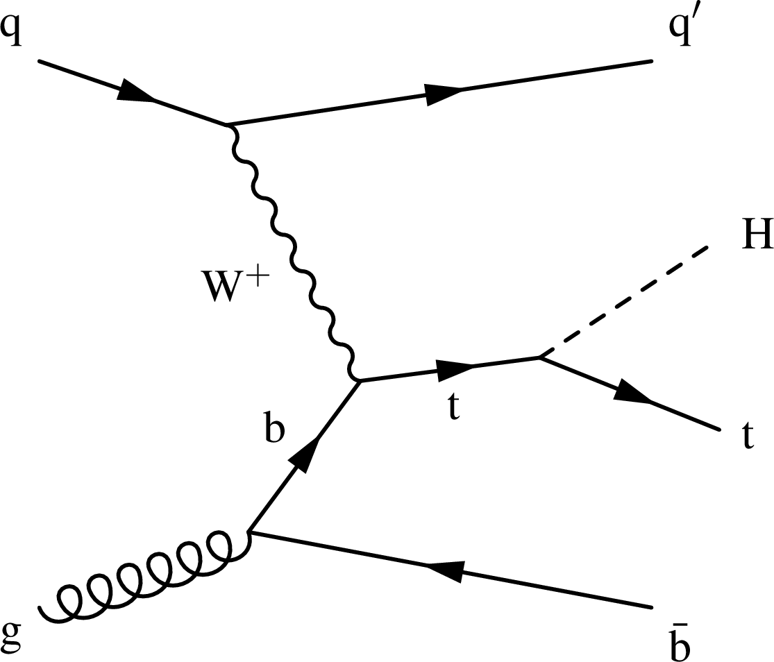
Figure 1-a:
Representative Feynman diagrams for the associated production of a single top quark and a Higgs boson in the $t$ channel (a,b) and in the tW channel (c,d). |
png pdf |
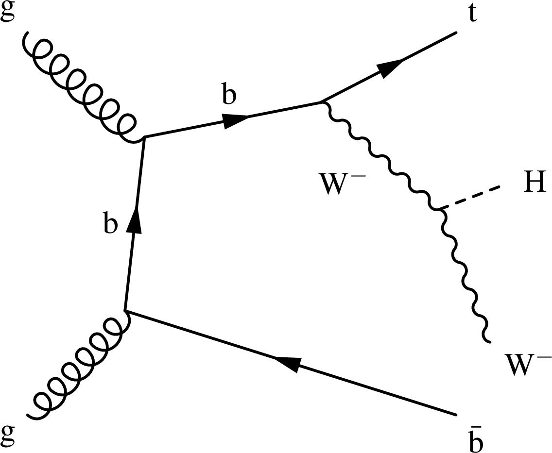
Figure 1-b:
Representative Feynman diagrams for the associated production of a single top quark and a Higgs boson in the $t$ channel (a,b) and in the tW channel (c,d). |
png pdf |
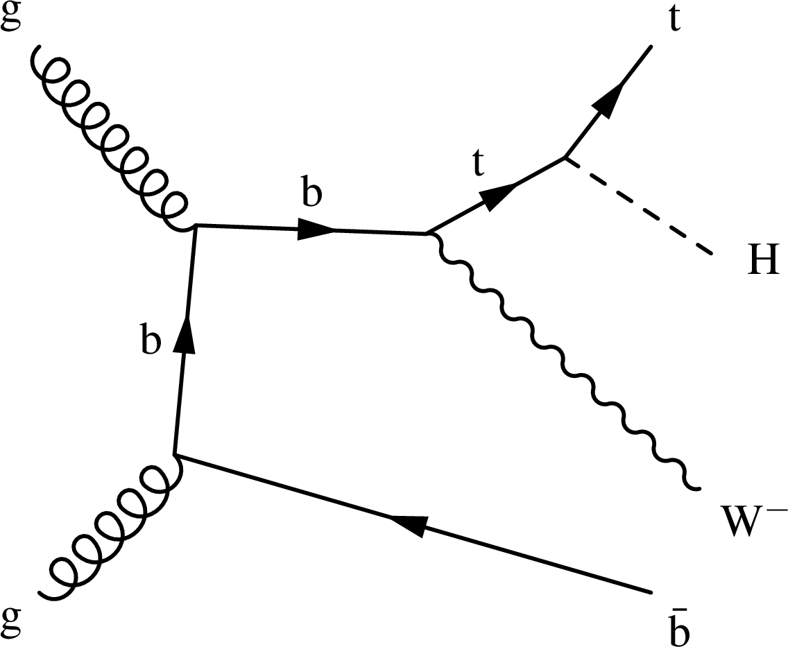
Figure 1-c:
Representative Feynman diagrams for the associated production of a single top quark and a Higgs boson in the $t$ channel (a,b) and in the tW channel (c,d). |
png pdf |
Figure 1-d:
Representative Feynman diagrams for the associated production of a single top quark and a Higgs boson in the $t$ channel (a,b) and in the tW channel (c,d). |
png pdf |
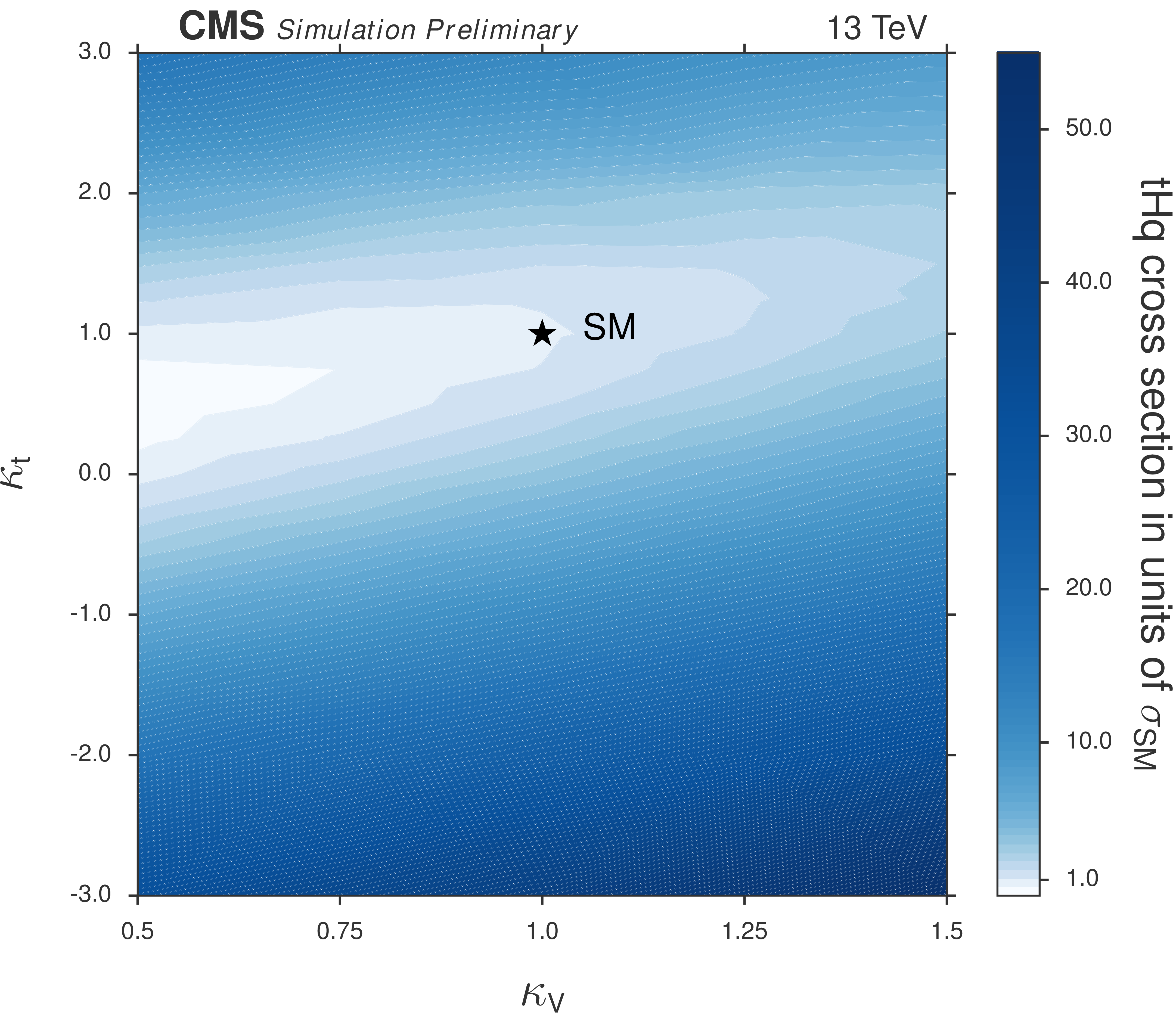
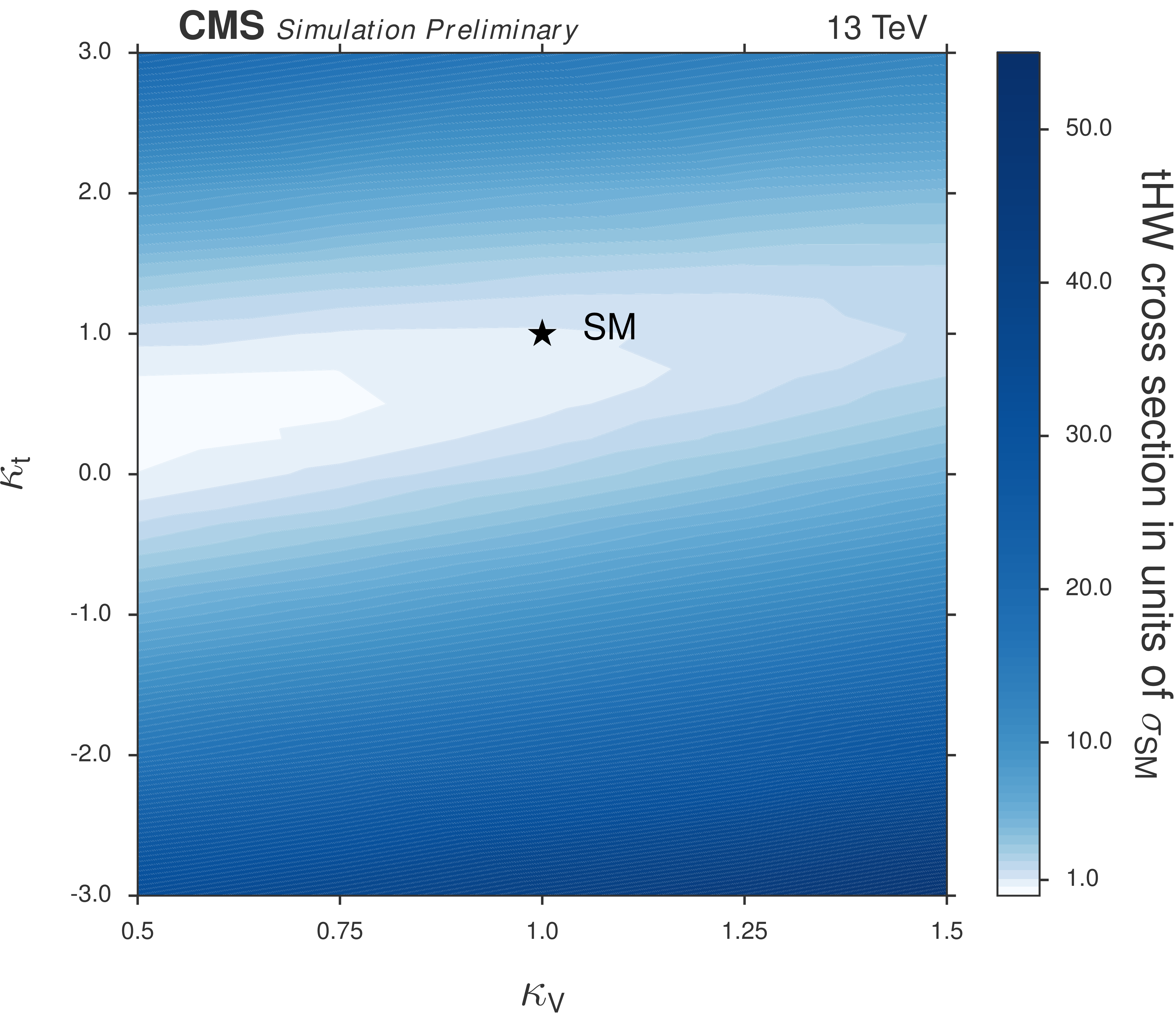
Figure 2-a:
Cross sections in the ${\kappa }_\text {t}-{\kappa }_\text {V}$ plane at 13 TeV for tHq (a) and tHW (b) production. Right figure adapted from [14]. |
png pdf |
Figure 2-b:
Cross sections in the ${\kappa }_\text {t}-{\kappa }_\text {V}$ plane at 13 TeV for tHq (a) and tHW (b) production. Right figure adapted from [14]. |
png pdf |
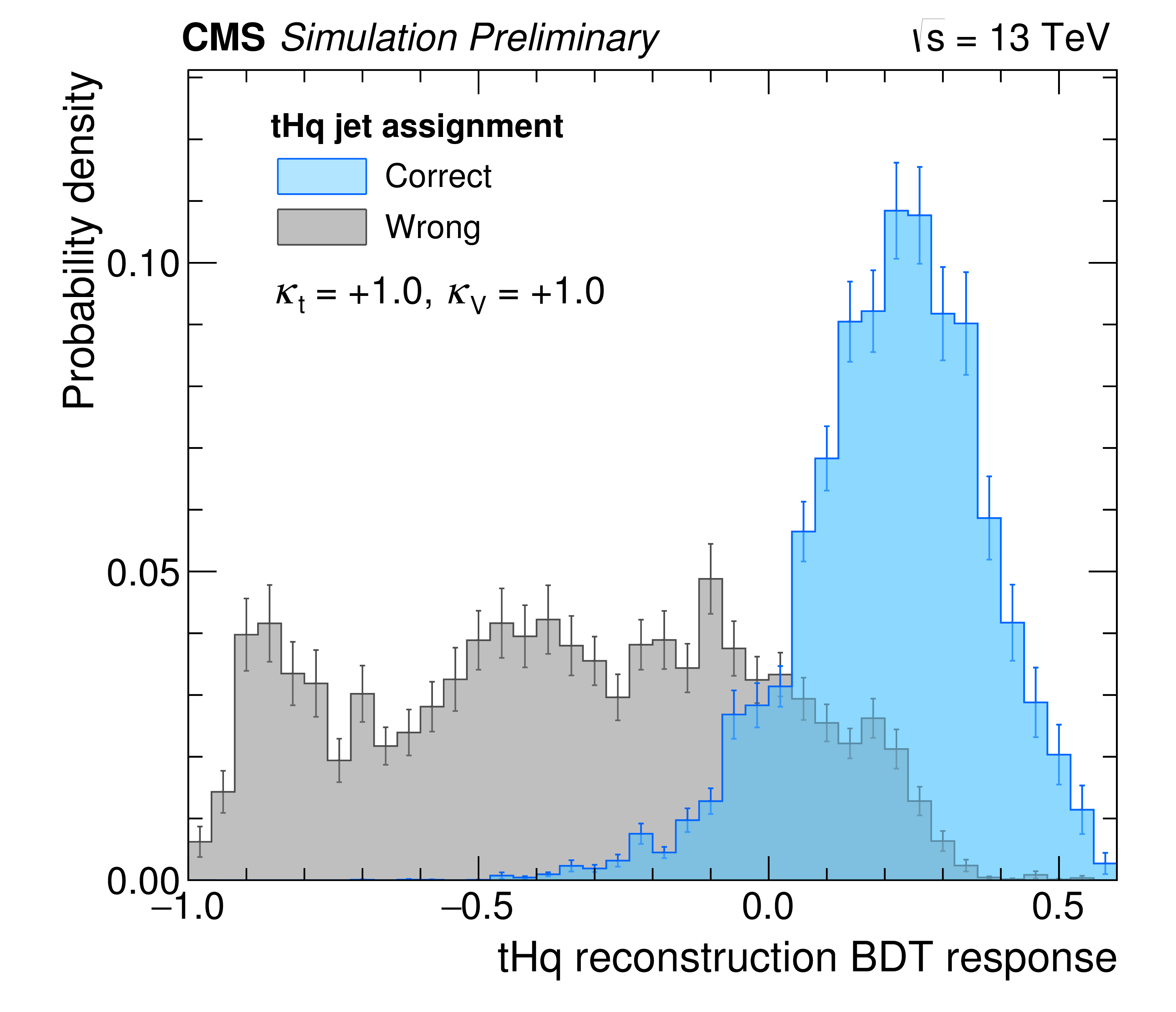
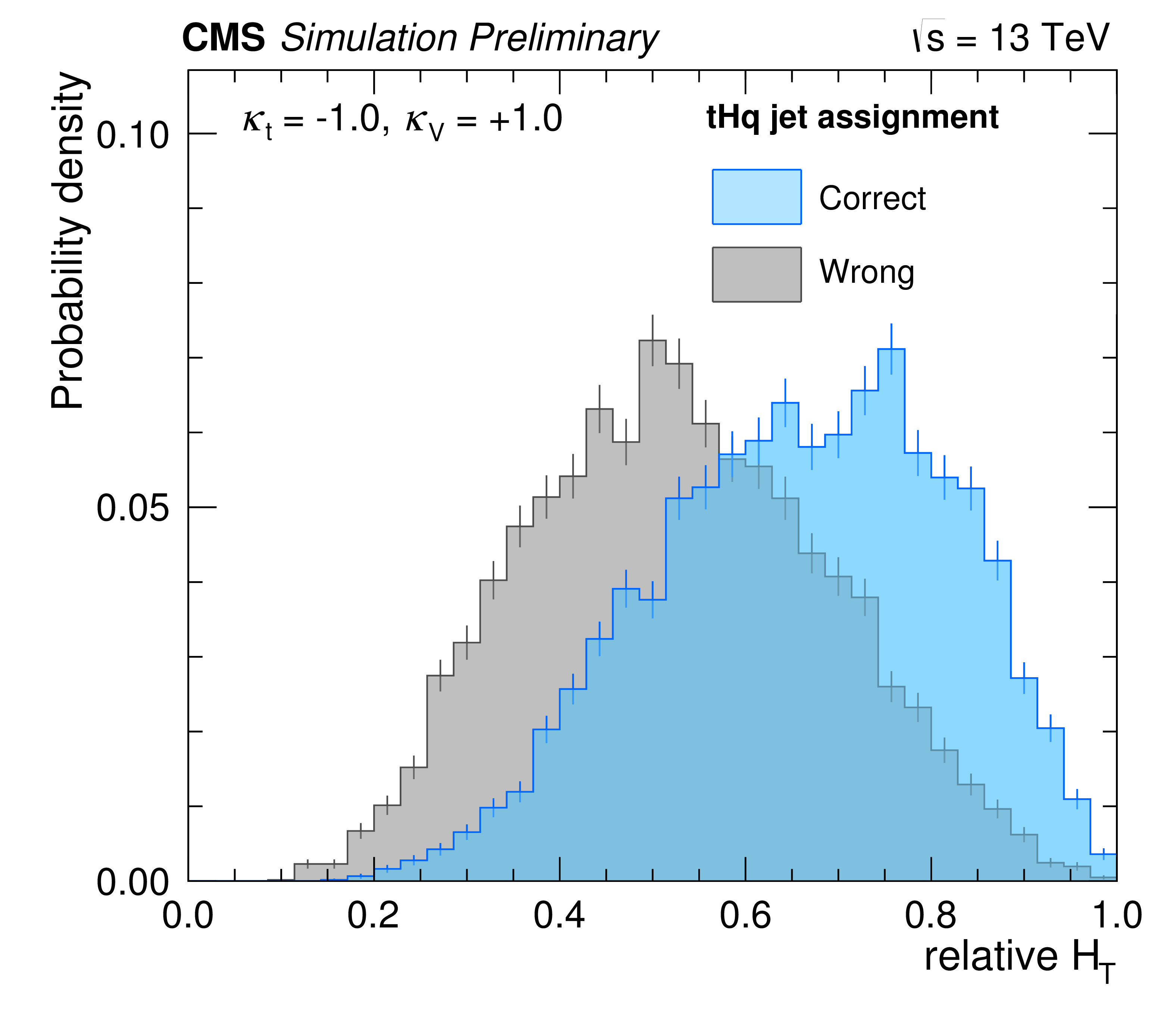
Figure 3-a:
Response of the ${\mathrm {t}} {\mathrm {H}} {\mathrm {q}}$ reconstruction classifier at 13 TeV |

png pdf |
Figure 3-b:
Response of the ${\mathrm {t}} {\mathrm {H}} {\mathrm {q}}$ reconstruction classifier at 13 TeV |
png pdf |
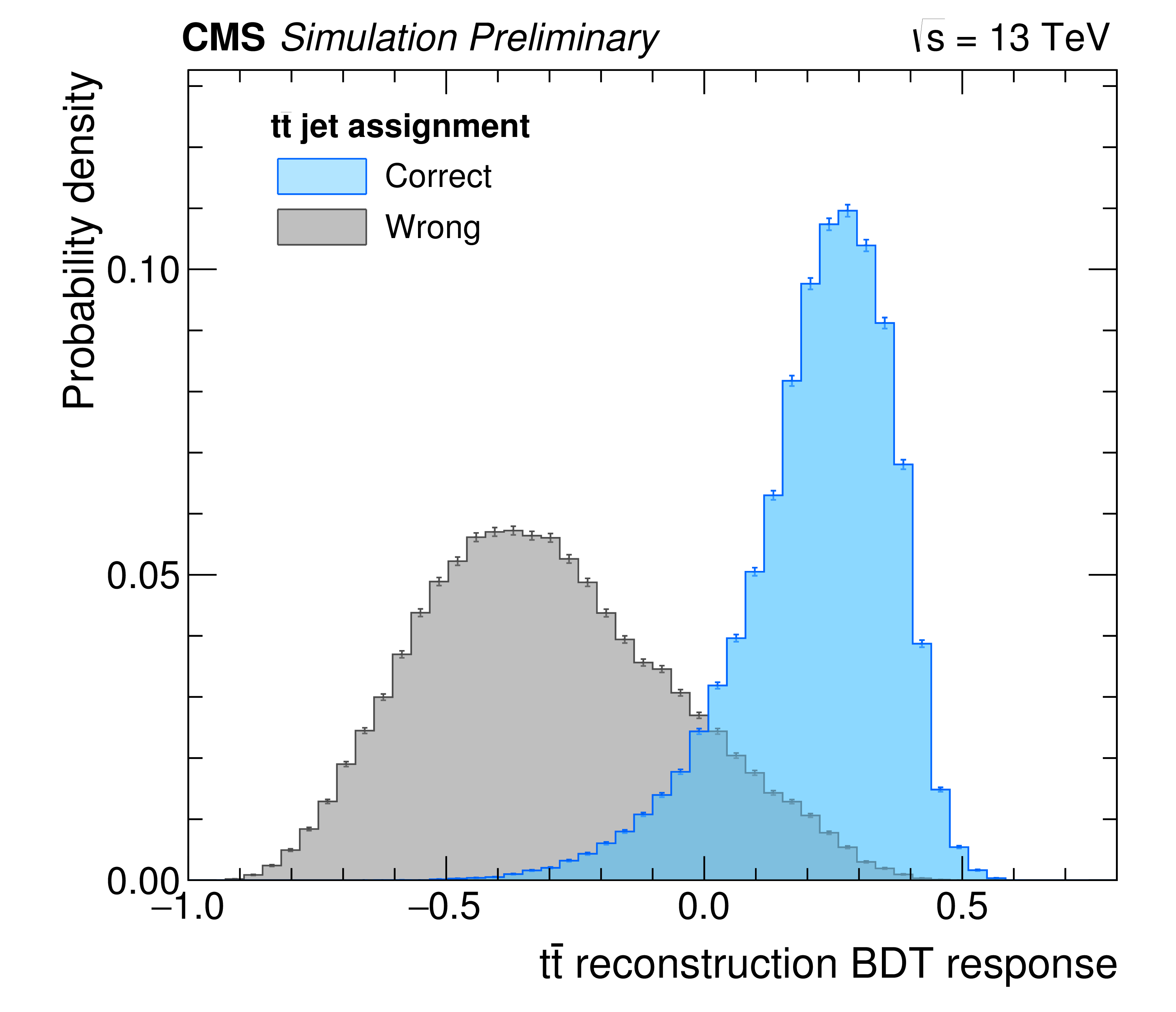
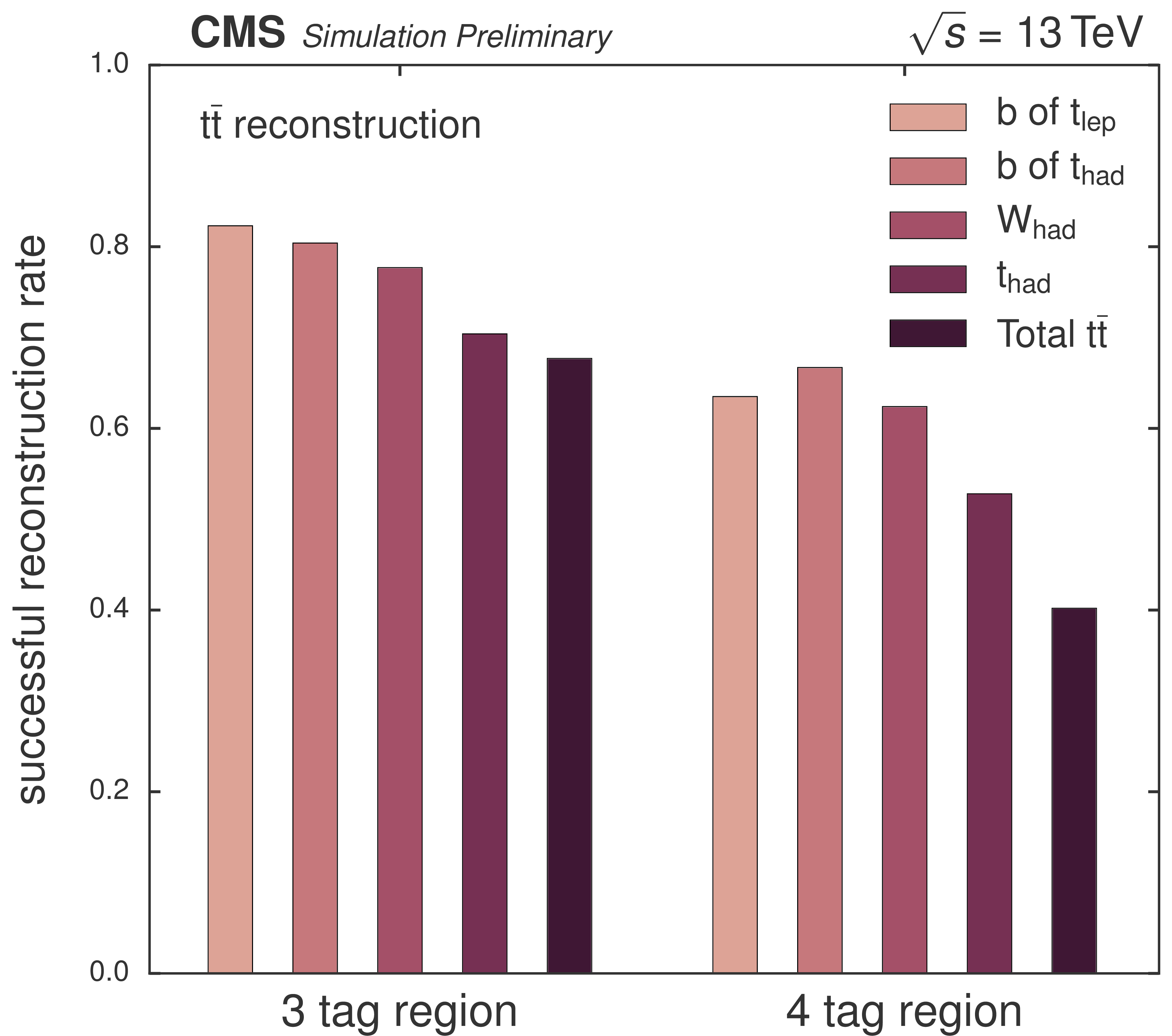
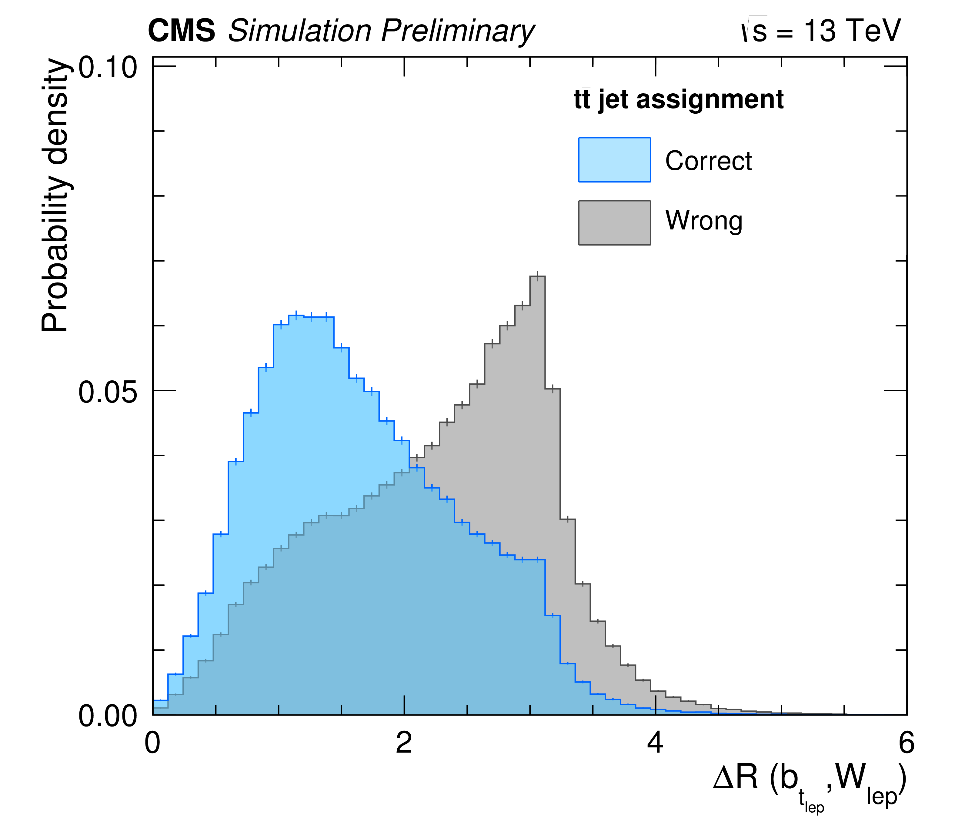
Figure 4:
Response of the ${\mathrm {t}\overline {\mathrm {t}}}$ reconstruction classifier at 13 TeV |
png pdf |
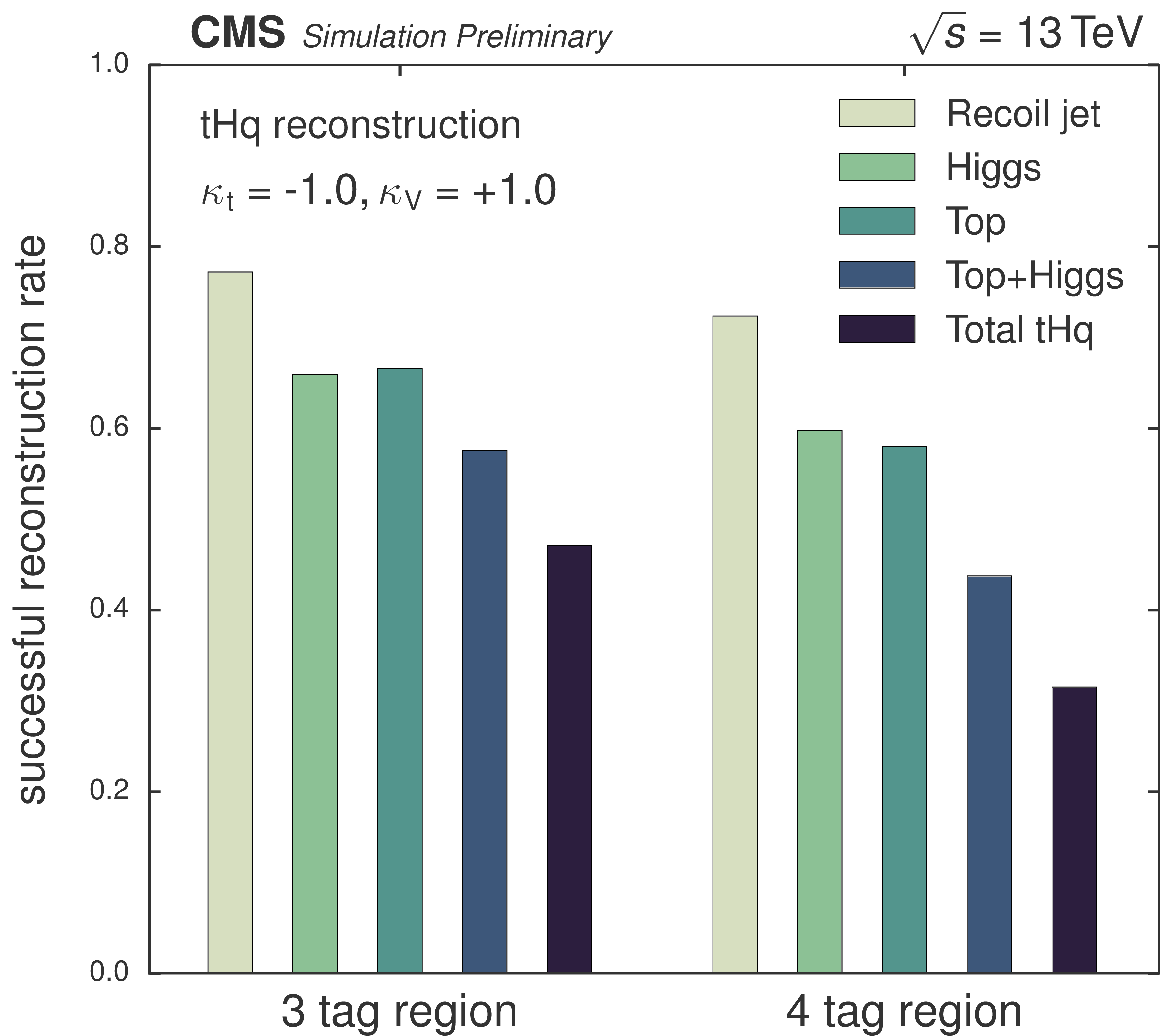
Figure 5-a:
Reconstruction efficiencies for different objects of the tHq process obtained from the tHq reconstruction in the 3 and 4 tag regions (a). Reconstruction efficiencies for different objects of the tt process obtained from the tt reconstruction in the 3 and 4 tag regions (b). |
png pdf |
Figure 5-b:
Reconstruction efficiencies for different objects of the tHq process obtained from the tHq reconstruction in the 3 and 4 tag regions (a). Reconstruction efficiencies for different objects of the tt process obtained from the tt reconstruction in the 3 and 4 tag regions (b). |
png pdf |
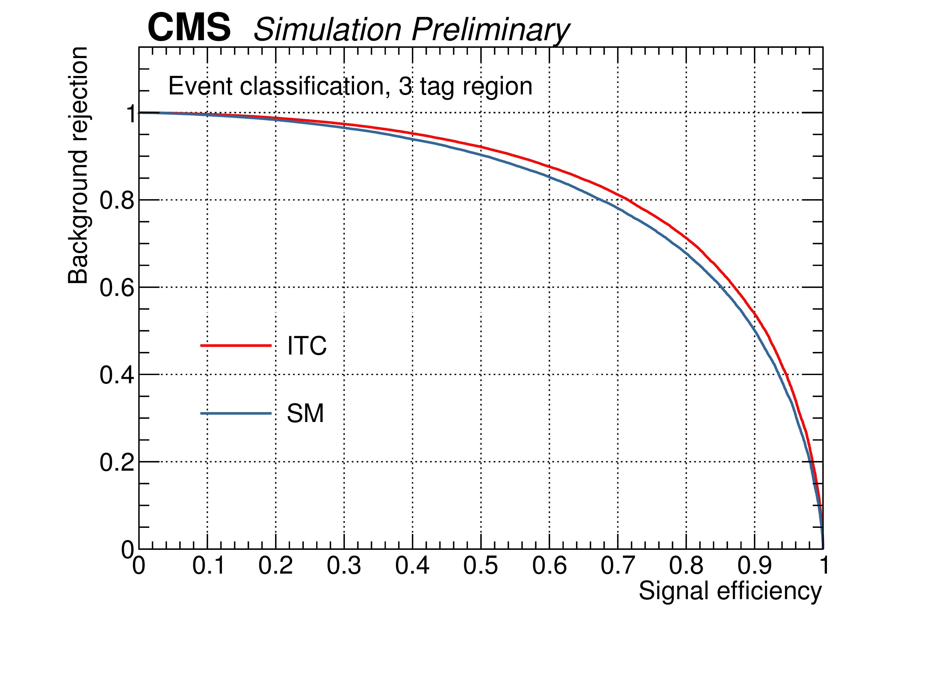
Figure 6-a:
ROC curve of the classification BDT for the SM and the ITC scenario in the 3 tag (a) and 4 tag (b) regions as examples for the 51 different classification BDTs. |

png pdf |
Figure 6-b:
ROC curve of the classification BDT for the SM and the ITC scenario in the 3 tag (a) and 4 tag (b) regions as examples for the 51 different classification BDTs. |
png pdf |
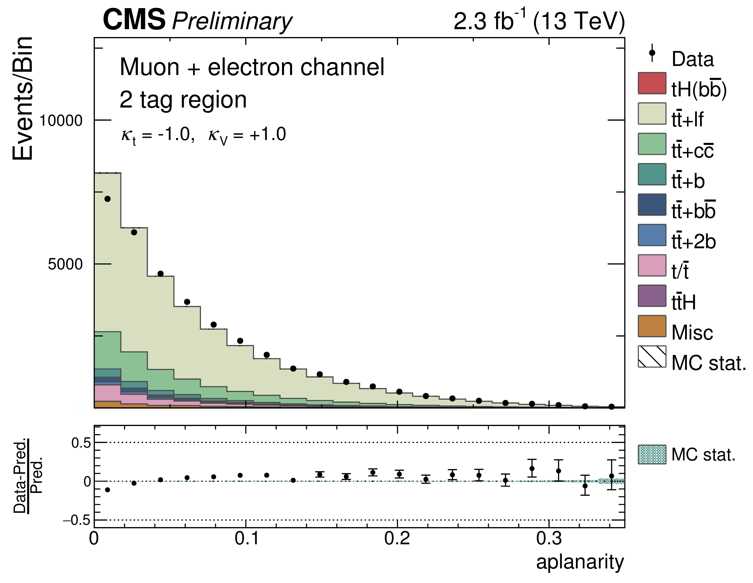
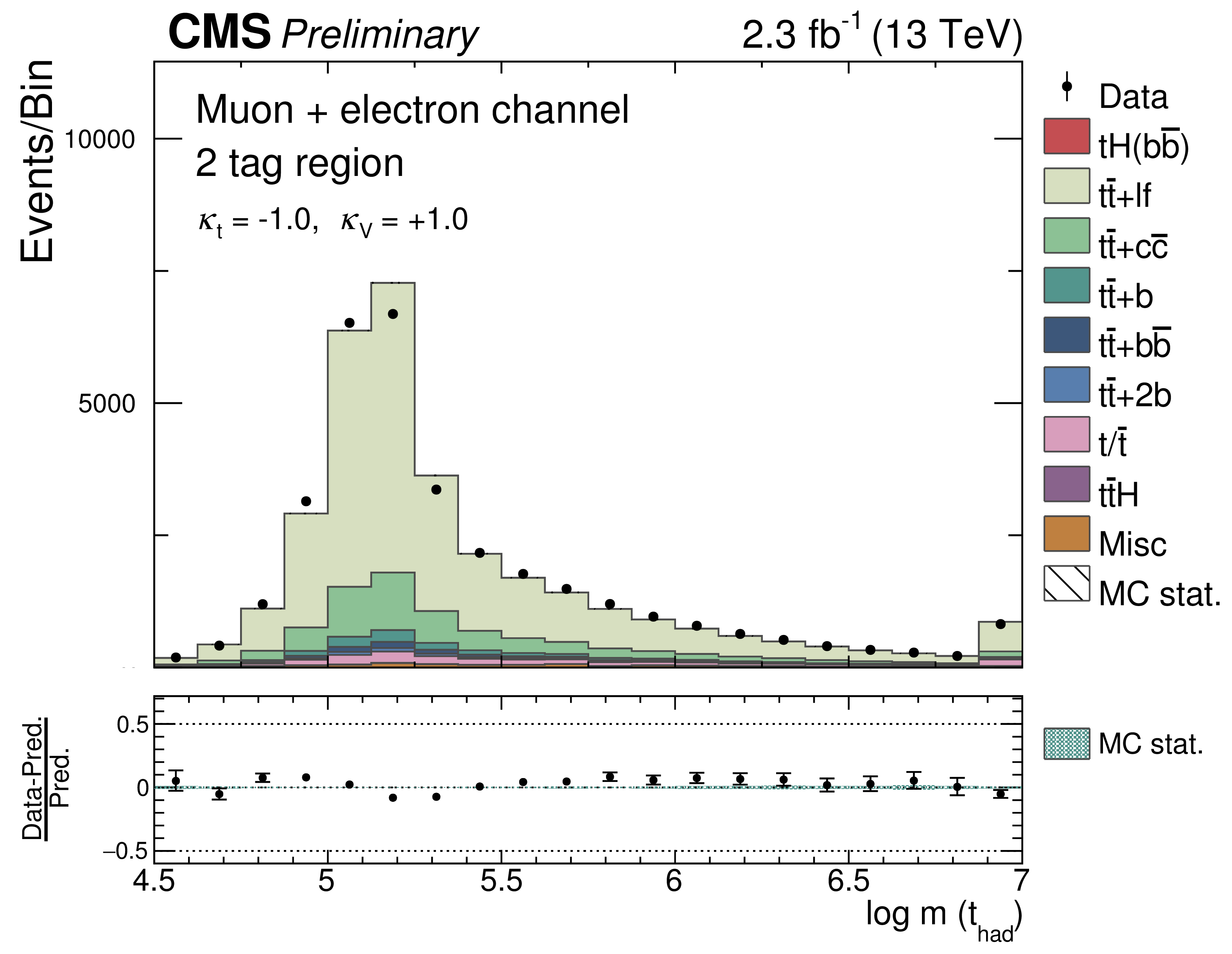
Figure 7-a:
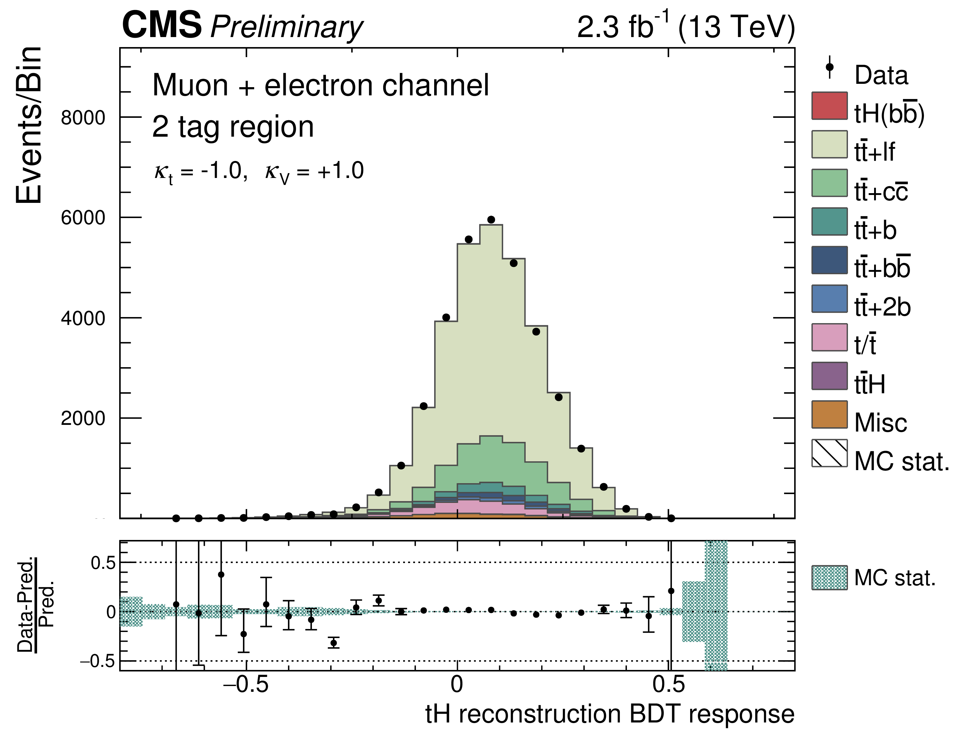
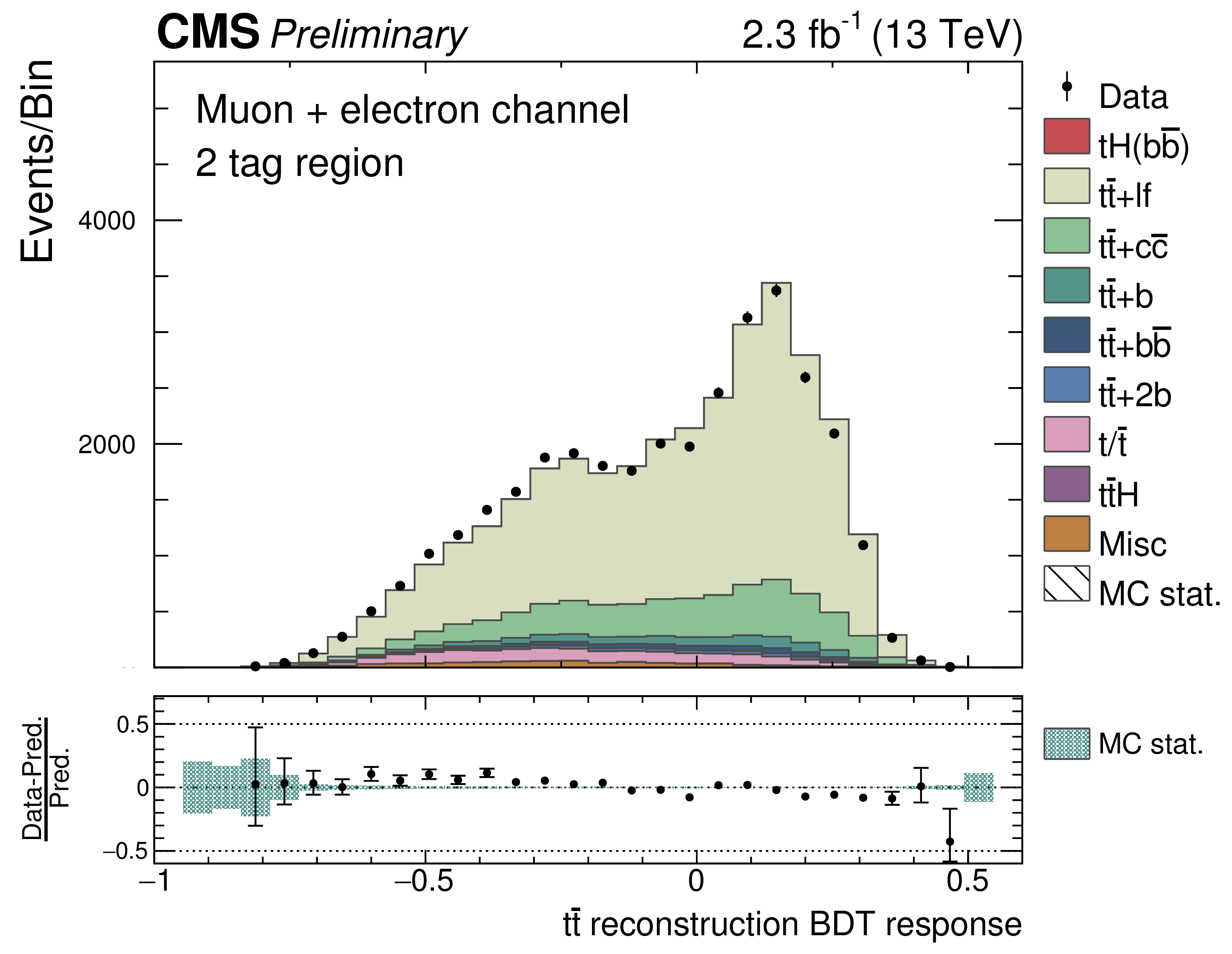
Simulation to data comparisons for the most discriminating variable of each category as shown in Table 4 (a,b,c) and the response distribution of the classification BDTs (d,e) in the 2 tag region at 13 TeV for the SM (d) and the ITC (e) case. The simulation is scaled to match the event yield observed in data. Contributions from ttZ, ttW, W+jets, and Z+jets are summarized under the category ?Misc?. |
png pdf |
Figure 7-b:
Simulation to data comparisons for the most discriminating variable of each category as shown in Table 4 (a,b,c) and the response distribution of the classification BDTs (d,e) in the 2 tag region at 13 TeV for the SM (d) and the ITC (e) case. The simulation is scaled to match the event yield observed in data. Contributions from ttZ, ttW, W+jets, and Z+jets are summarized under the category ?Misc?. |

png pdf |
Figure 7-c:
Simulation to data comparisons for the most discriminating variable of each category as shown in Table 4 (a,b,c) and the response distribution of the classification BDTs (d,e) in the 2 tag region at 13 TeV for the SM (d) and the ITC (e) case. The simulation is scaled to match the event yield observed in data. Contributions from ttZ, ttW, W+jets, and Z+jets are summarized under the category ?Misc?. |

png pdf |
Figure 7-d:
Simulation to data comparisons for the most discriminating variable of each category as shown in Table 4 (a,b,c) and the response distribution of the classification BDTs (d,e) in the 2 tag region at 13 TeV for the SM (d) and the ITC (e) case. The simulation is scaled to match the event yield observed in data. Contributions from ttZ, ttW, W+jets, and Z+jets are summarized under the category ?Misc?. |
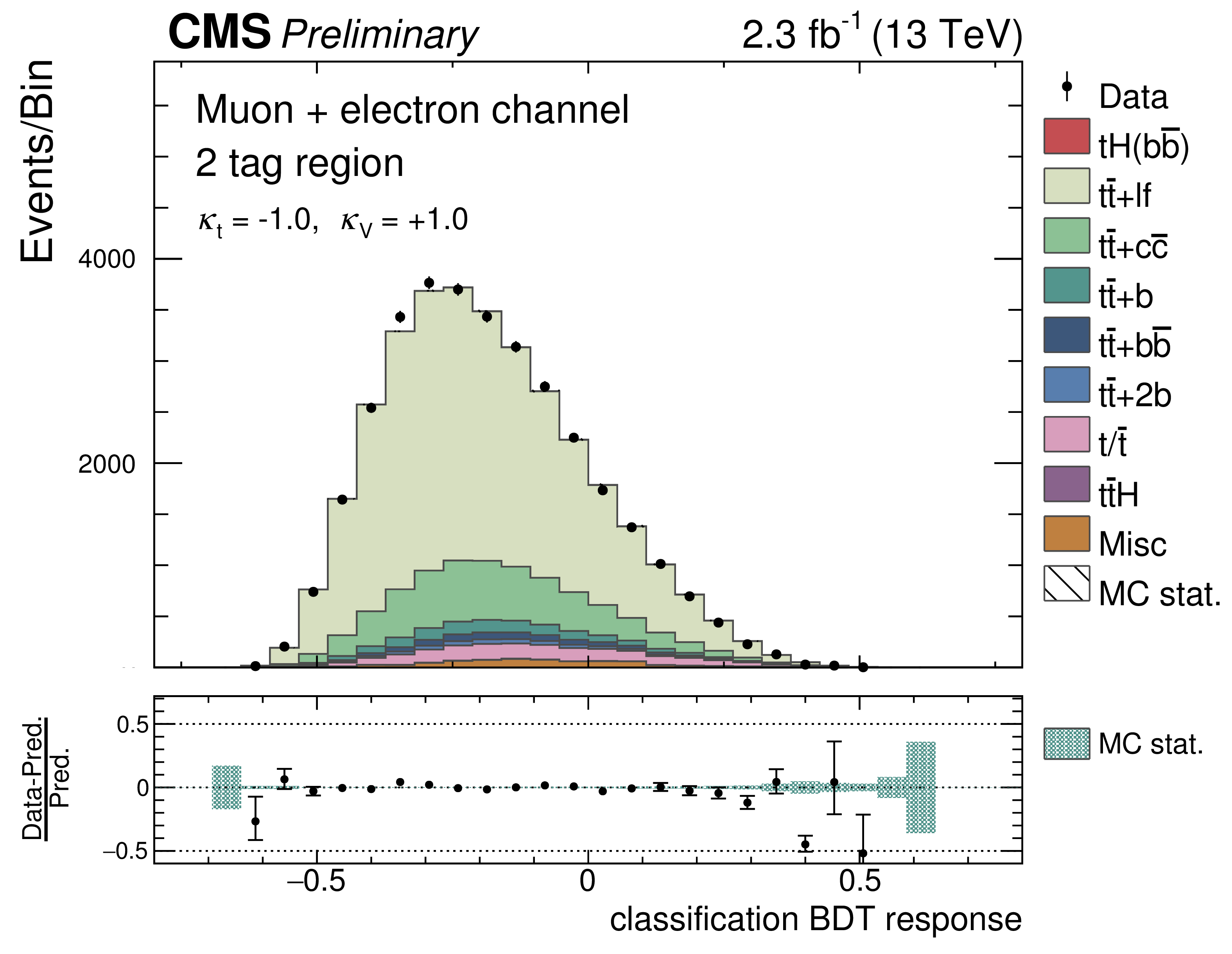
png pdf |
Figure 7-e:
Simulation to data comparisons for the most discriminating variable of each category as shown in Table 4 (a,b,c) and the response distribution of the classification BDTs (d,e) in the 2 tag region at 13 TeV for the SM (d) and the ITC (e) case. The simulation is scaled to match the event yield observed in data. Contributions from ttZ, ttW, W+jets, and Z+jets are summarized under the category ?Misc?. |
png pdf |
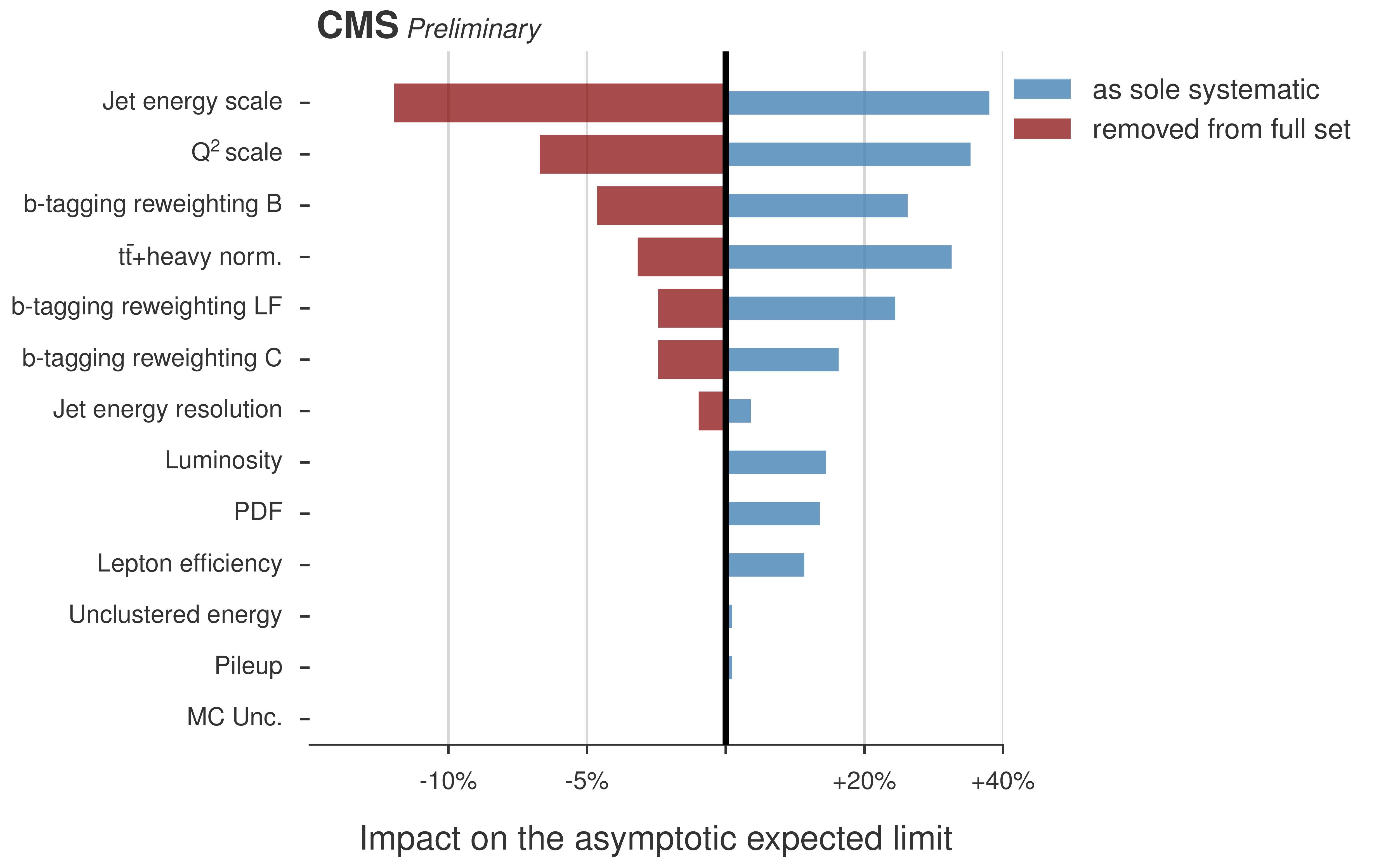
Figure 8:
Impact of groups of systematic uncertainties on the expected asymptotic limit. The groups of systematic uncertainties are either removed from the fit by fixing them to their postfit values, or used as single systematic uncertainty by fixing all other uncertainties to their postfit values. The changes displayed in this diagram are calculated relative to the limit with all systematic uncertainties included (red bars) and to the limit where all uncertainties are fixed to their best fit values (blue bars). |

png pdf |
Figure 9-a:
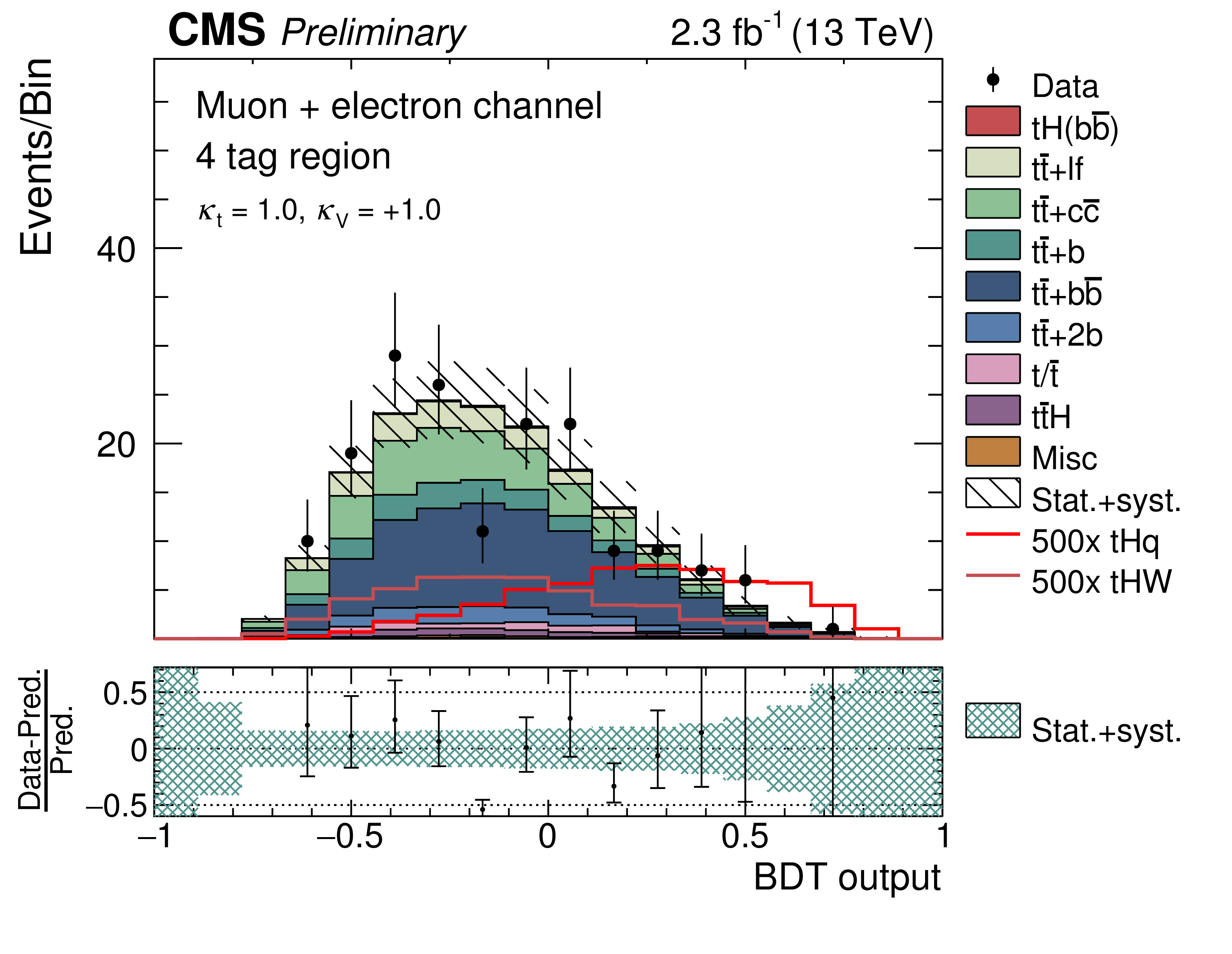
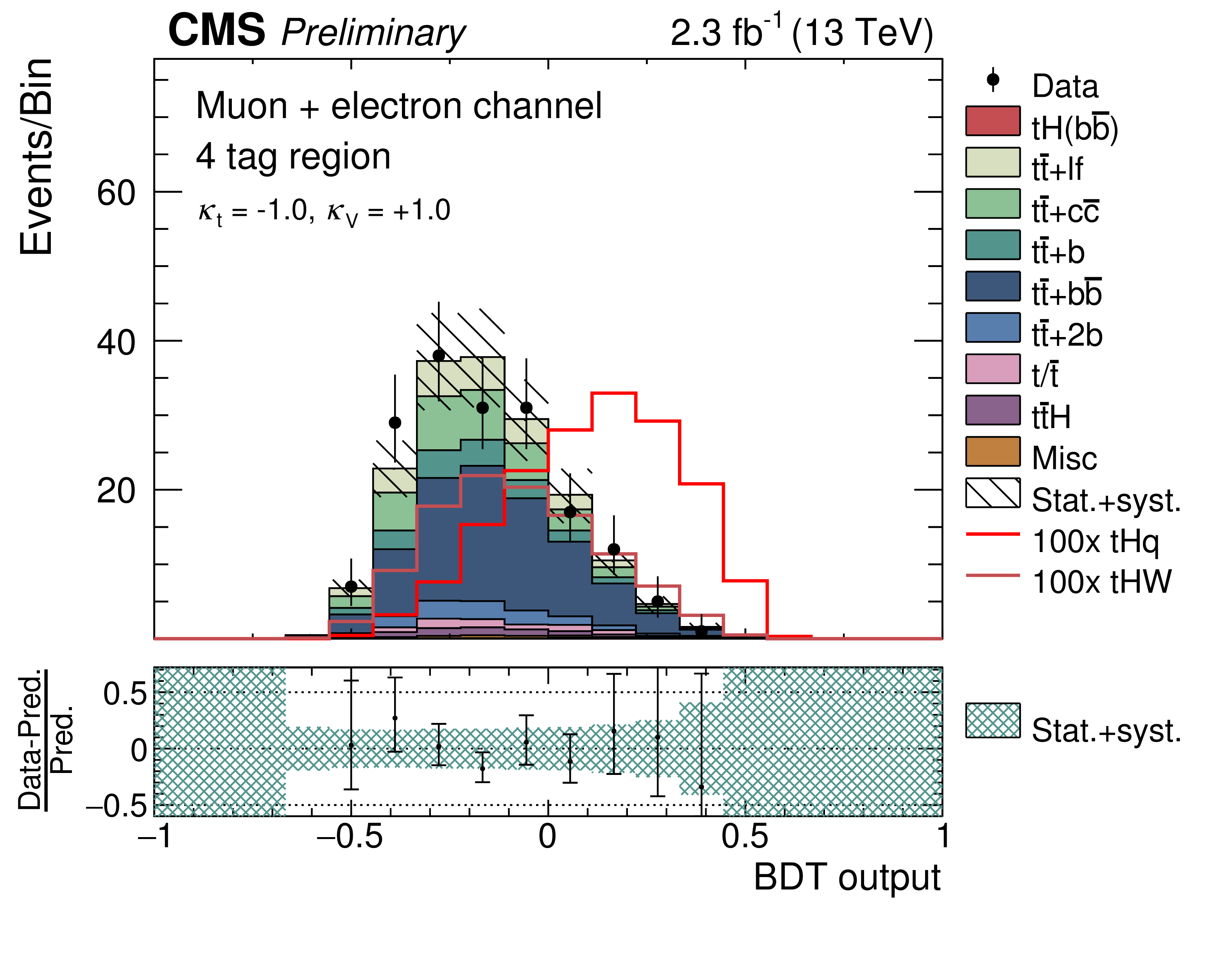
Postfit distributions of the classification BDT response in the 3 tag (a,c) and 4 tag (b,d) regions for the SM (a,b) and ITC (c,d) coupling scenarios. The uncertainty bands contain both systematic and statistical contributions. The signal distributions correspond to the expected contributions scaled by the factors given in the legends. |
png pdf |
Figure 9-b:
Postfit distributions of the classification BDT response in the 3 tag (a,c) and 4 tag (b,d) regions for the SM (a,b) and ITC (c,d) coupling scenarios. The uncertainty bands contain both systematic and statistical contributions. The signal distributions correspond to the expected contributions scaled by the factors given in the legends. |
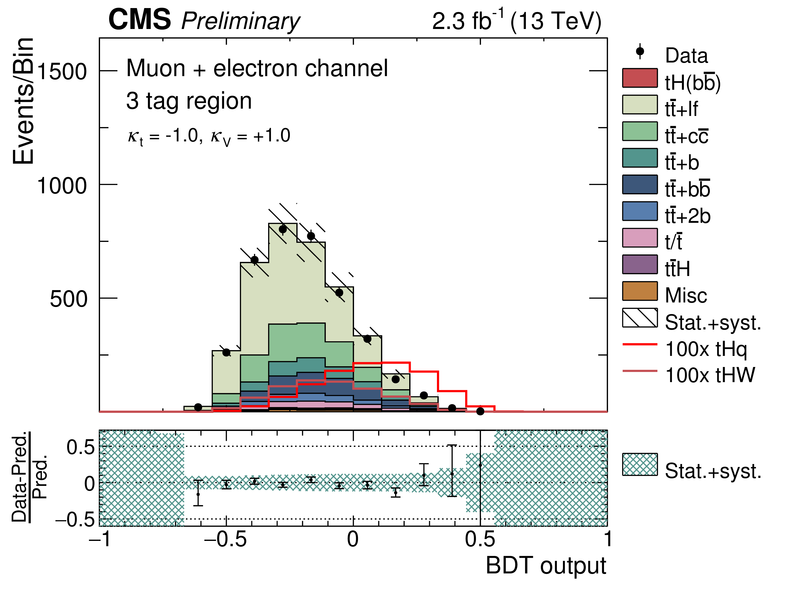
png pdf |
Figure 9-c:
Postfit distributions of the classification BDT response in the 3 tag (a,c) and 4 tag (b,d) regions for the SM (a,b) and ITC (c,d) coupling scenarios. The uncertainty bands contain both systematic and statistical contributions. The signal distributions correspond to the expected contributions scaled by the factors given in the legends. |
png pdf |
Figure 9-d:
Postfit distributions of the classification BDT response in the 3 tag (a,c) and 4 tag (b,d) regions for the SM (a,b) and ITC (c,d) coupling scenarios. The uncertainty bands contain both systematic and statistical contributions. The signal distributions correspond to the expected contributions scaled by the factors given in the legends. |
png pdf |
Figure 10-a:
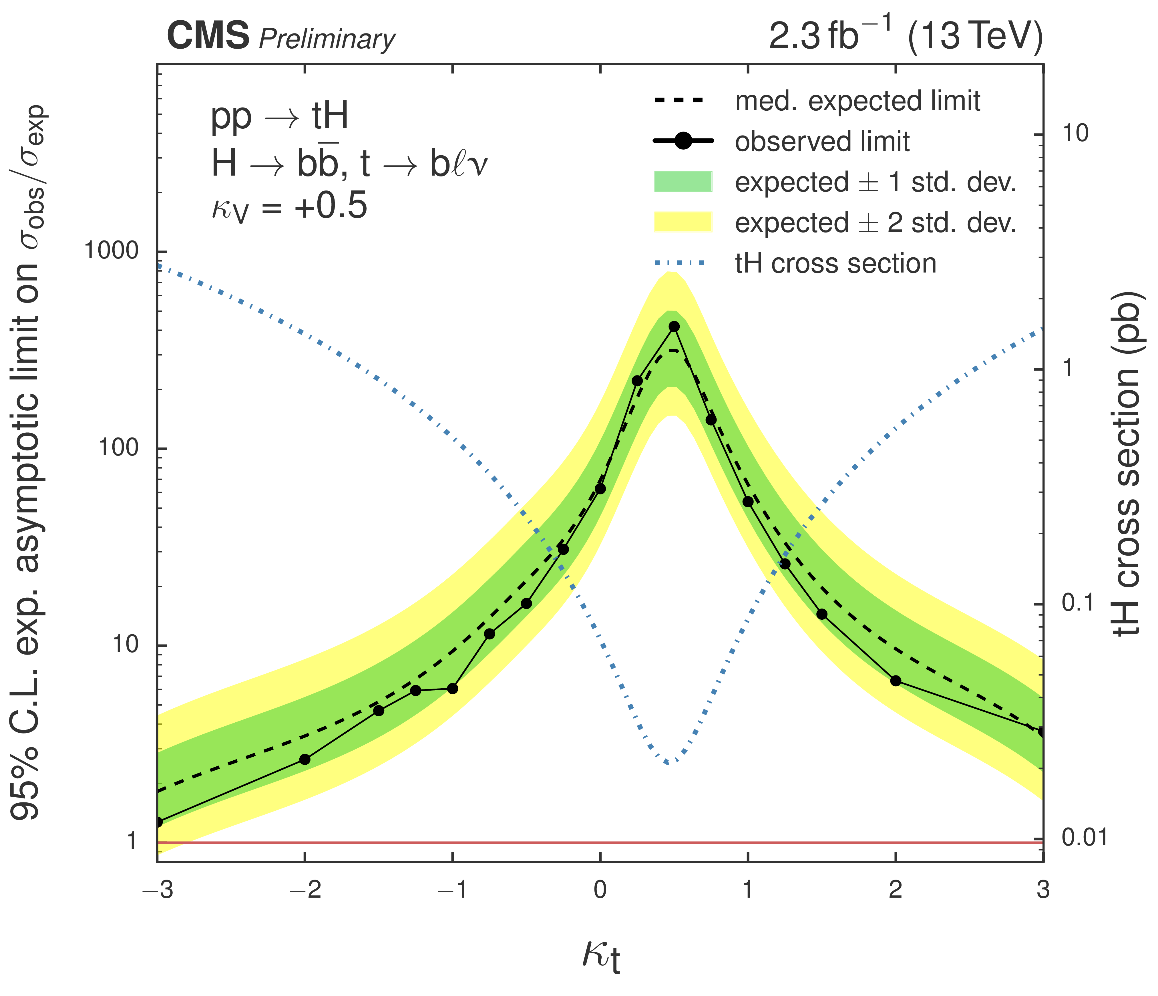
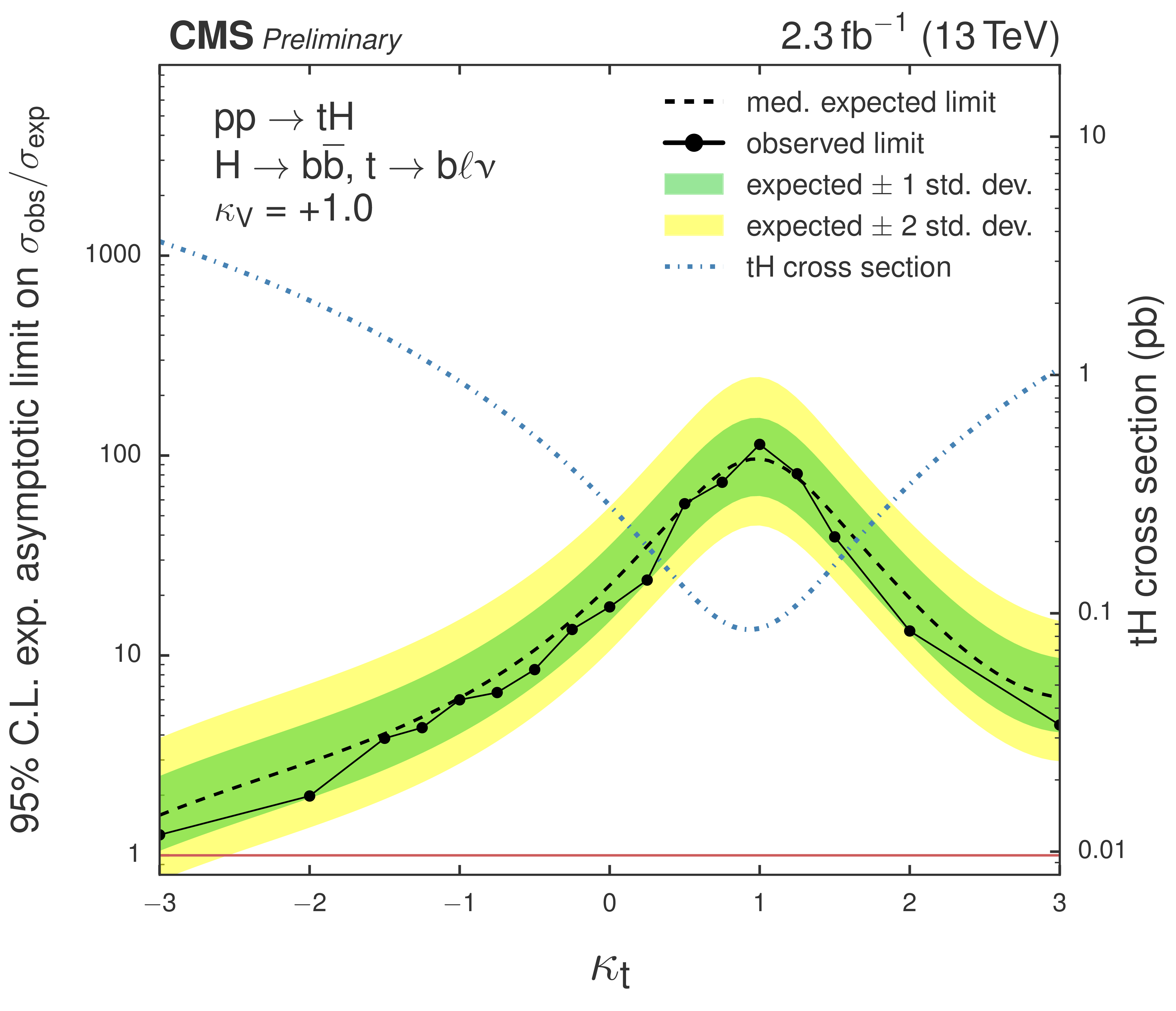
Upper limits on tH scenarios with different $\kappa _\text {t} - \kappa _\text {V}$ configurations, for $\kappa _\text {V}=+0.5$ (a), $\kappa _\text {V}=+1$ (b), and $\kappa _\text {V}=+1.5$ (c). In addition also the tH cross sections are given (right $y$ axis). |
png pdf |
Figure 10-b:
Upper limits on tH scenarios with different $\kappa _\text {t} - \kappa _\text {V}$ configurations, for $\kappa _\text {V}=+0.5$ (a), $\kappa _\text {V}=+1$ (b), and $\kappa _\text {V}=+1.5$ (c). In addition also the tH cross sections are given (right $y$ axis). |
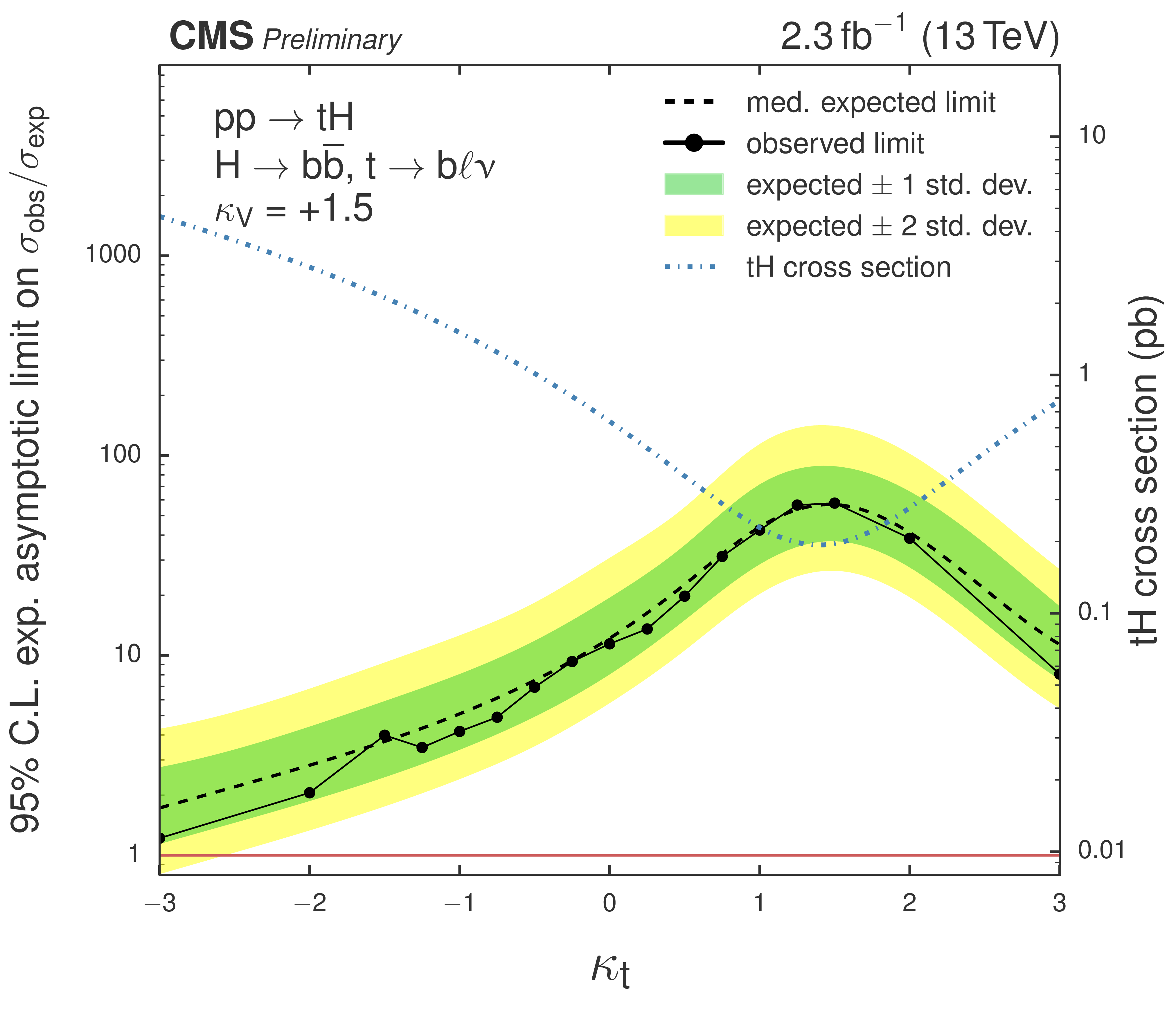
png pdf |
Figure 10-c:
Upper limits on tH scenarios with different $\kappa _\text {t} - \kappa _\text {V}$ configurations, for $\kappa _\text {V}=+0.5$ (a), $\kappa _\text {V}=+1$ (b), and $\kappa _\text {V}=+1.5$ (c). In addition also the tH cross sections are given (right $y$ axis). |
| Tables | |
png pdf |
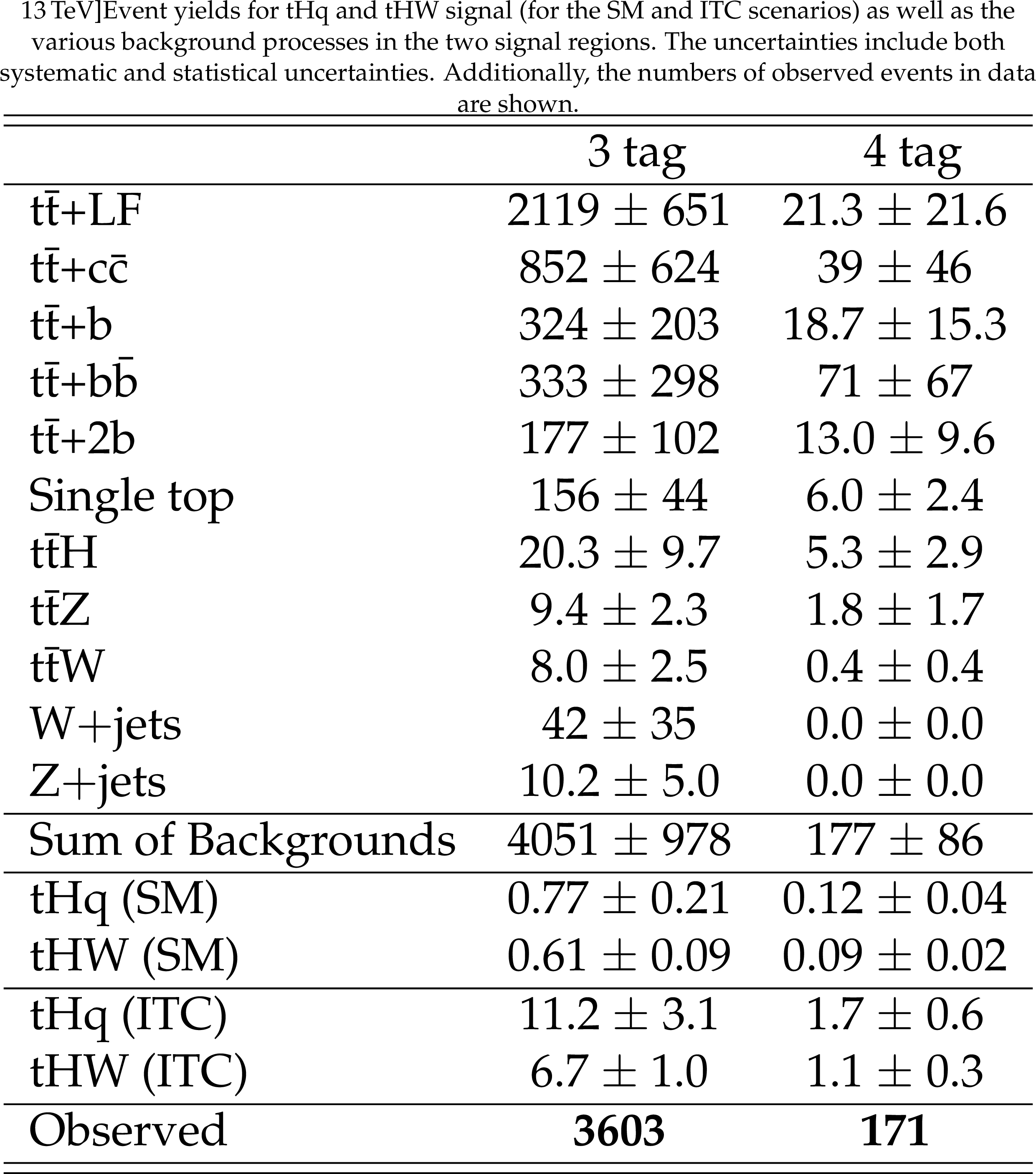
Table 1:
Event yields for tHq and tHW signal (for the SM and ITC scenarios) as well as the various background processes in the two signal regions. The uncertainties include both systematic and statistical uncertainties. Additionally, the numbers of observed events in data are shown. |
png pdf |
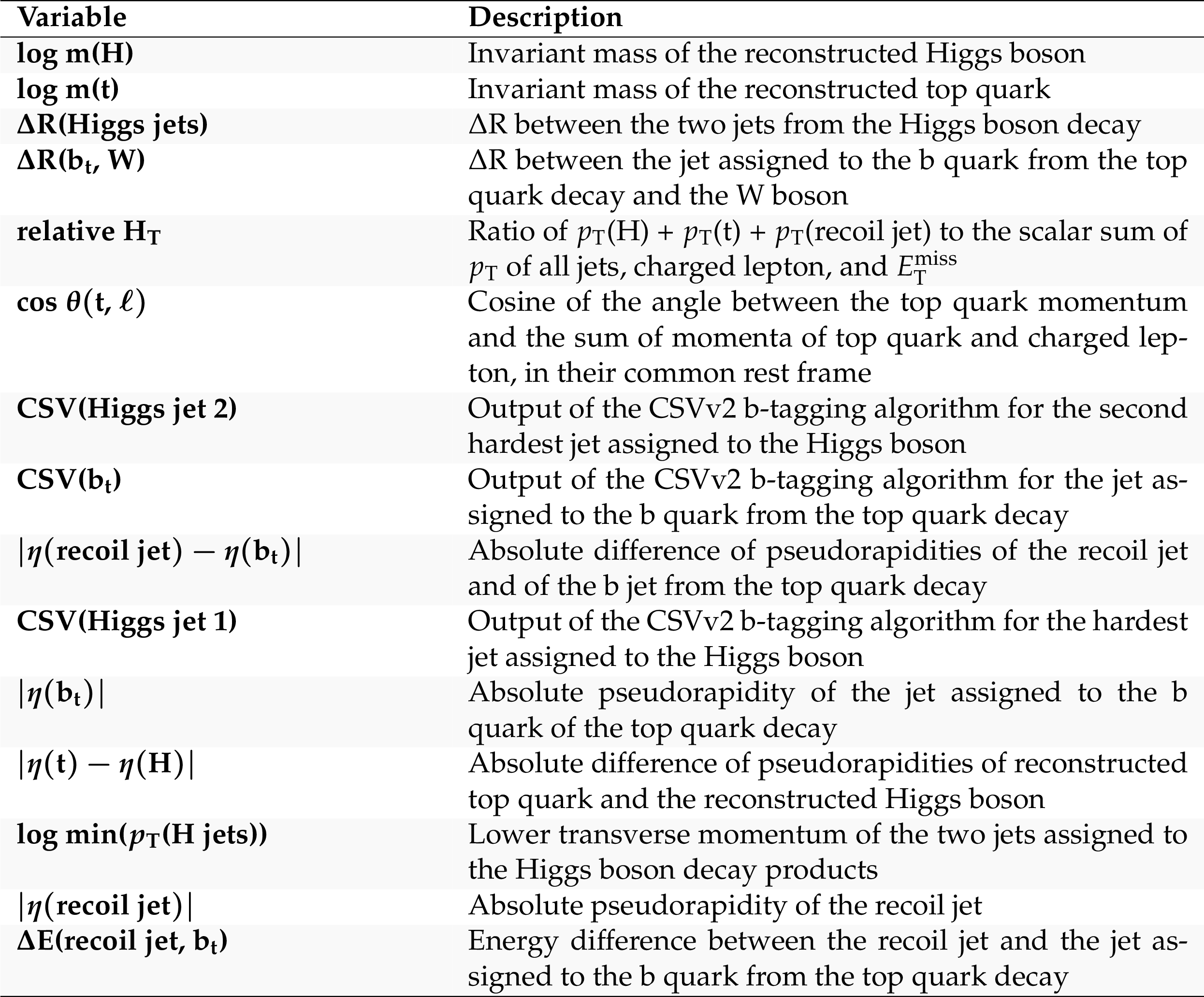
Table 2 :
Input variables for the jet-assignment BDT under the tHq hypothesis sorted by their importance in the training. |
png pdf |
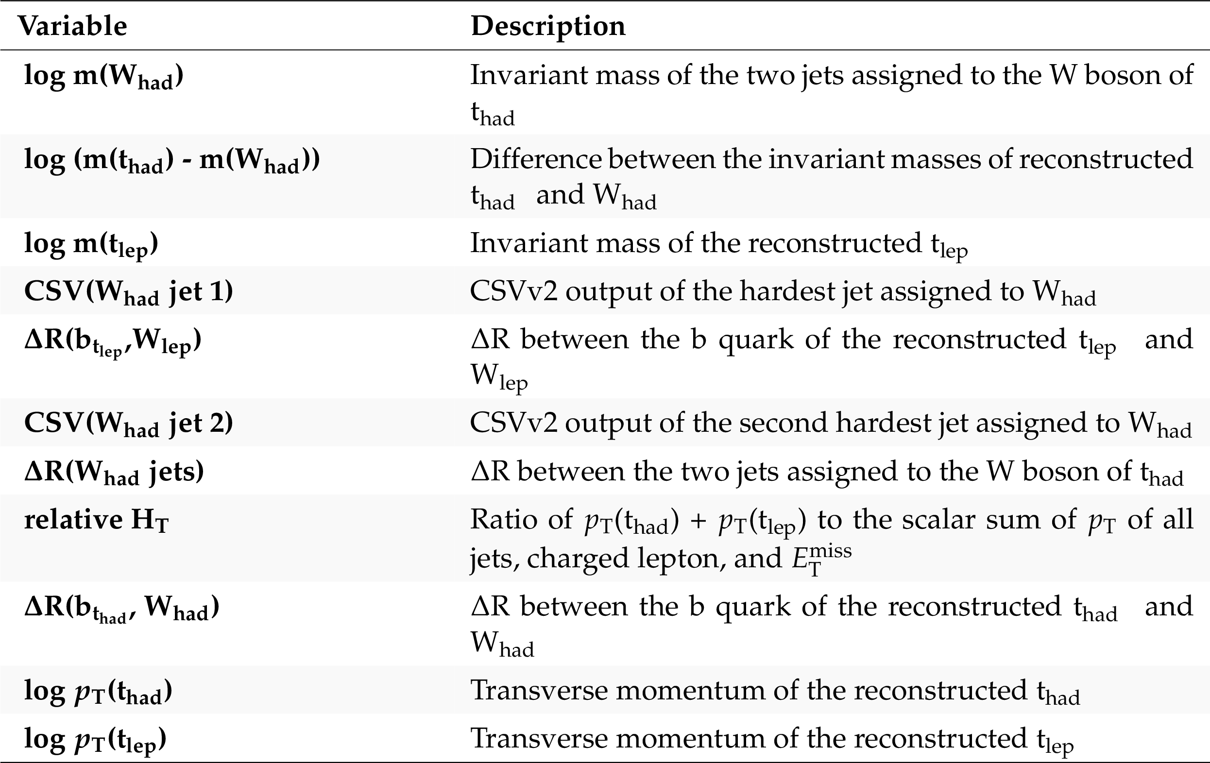
Table 3:
Input variables for the jet-assignment BDT under the tt hypothesis sorted by their importance in the training. The hadronically and leptonically decaying W bosons and top quarks are labeled with $\mathrm{W_{had}}$, $\mathrm{W_{lep}}$, $\mathrm{t_{had}}$, and $\mathrm{t_{lep}}$. |
png pdf |
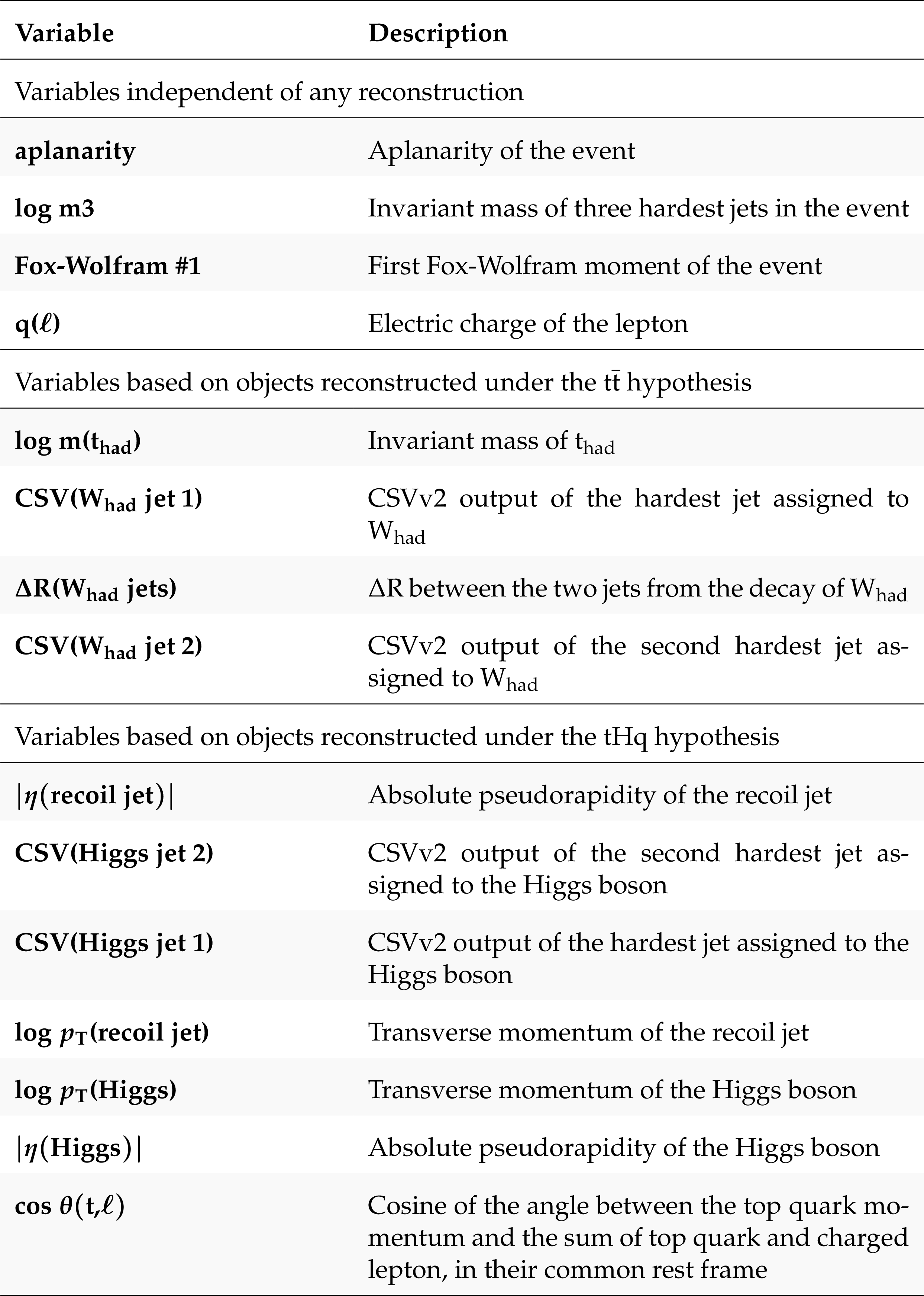
Table 4:
Input variables used in the classification, ranked by their importance within each category. |
png pdf |
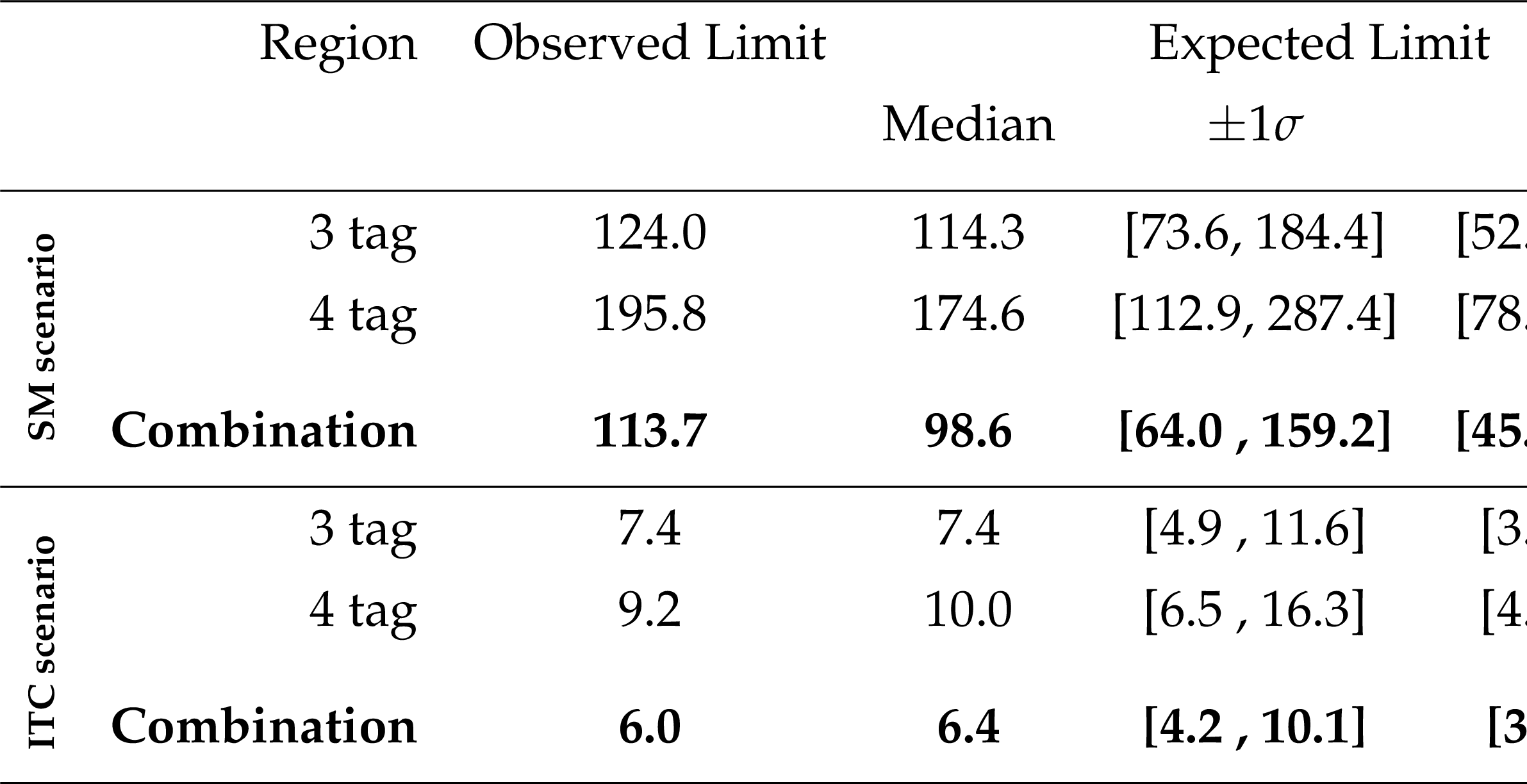
Table 5:
Expected and observed asymptotic CLs limits at 95% CL in the 3 tag and 4 tag regions and their combination for the SM and ITC coupling scenarios. Also the 68% and 95% uncertainty band values are shown. |
| Summary |
| A search for $t$- and tW-channel single top quark production in association with the 125 GeV Higgs boson has been conducted using the 2015 CMS dataset at a center-of-mass energy of 13 TeV. For the first time the tW channel has been included. The analysis focuses on possible variations in the coupling between the Higgs boson and the top quark or the W boson to search for deviations from the standard model. Exclusion limits are calculated as a function of the coupling strength factors $\kappa_\text{t}$ and $\kappa_\text{V}$. Two different signal regions are selected: one region with at least 4 jets, among them exactly 3 b-tagged jets; the other region with at least 5 jets, exactly 4 of which are b-tagged. An identification of jets in the final state under the $\mathrm{t }\mathrm{ H }\mathrm{q}$ or $\mathrm{ t \bar{t} }$ hypothesis is performed using two separate sets of reconstruction BDTs. A consecutive set of classification BDTs uses variables derived in these assignments to enhance the signal-to-background ratio and discriminate against main backgrounds, including the predominant $\mathrm{ t \bar{t} }$ production. Limits are then calculated using the distributions of the responses of the classification BDTs. The observed (expected) 95% confidence level upper limit for the standard model is 113.7$\times \sigma_{\mathrm{SM}}$ (98.6$\times\sigma_{\mathrm{SM}}$) and the 95% confidence-level upper limit for the inverted top coupling scenario is 6.0 times the predicted cross section, with an expected upper limit of 6.4. |
| Additional Figures | |

png pdf |
Additional Figure 1:
Kinematics of the tHq process at LO at $\sqrt {s} = $ 13 TeV for $\kappa _{\mathrm {t}} = -1.0$: Rapidity versus transverse momentum of the Higgs boson. |
png pdf |
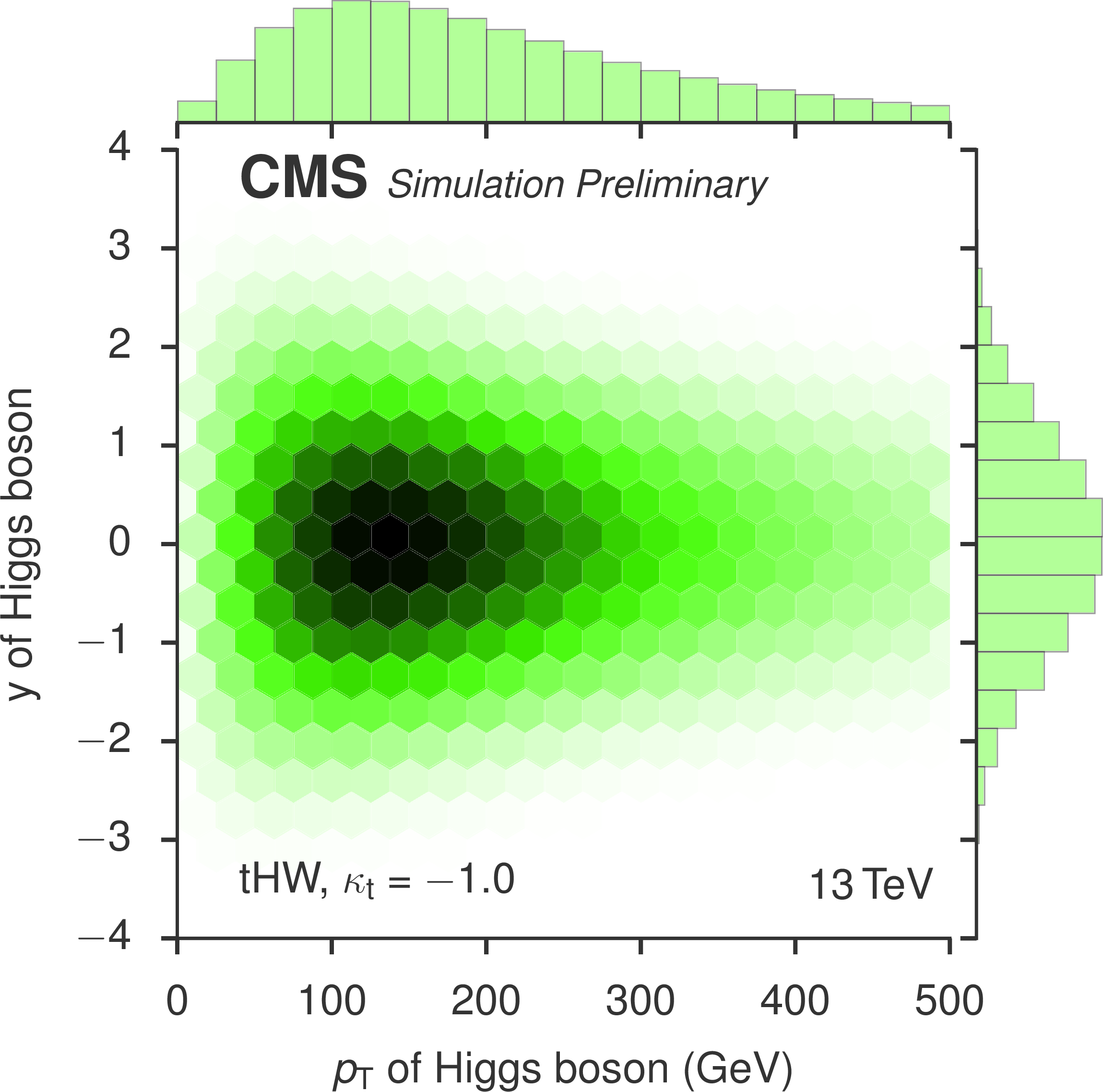
Additional Figure 2:
Kinematics of the tHW process at LO at $\sqrt {s} =$ 13 TeV for $\kappa _{\mathrm {t}} = -1.0$: Rapidity versus transverse momentum of the Higgs boson. |
png pdf |
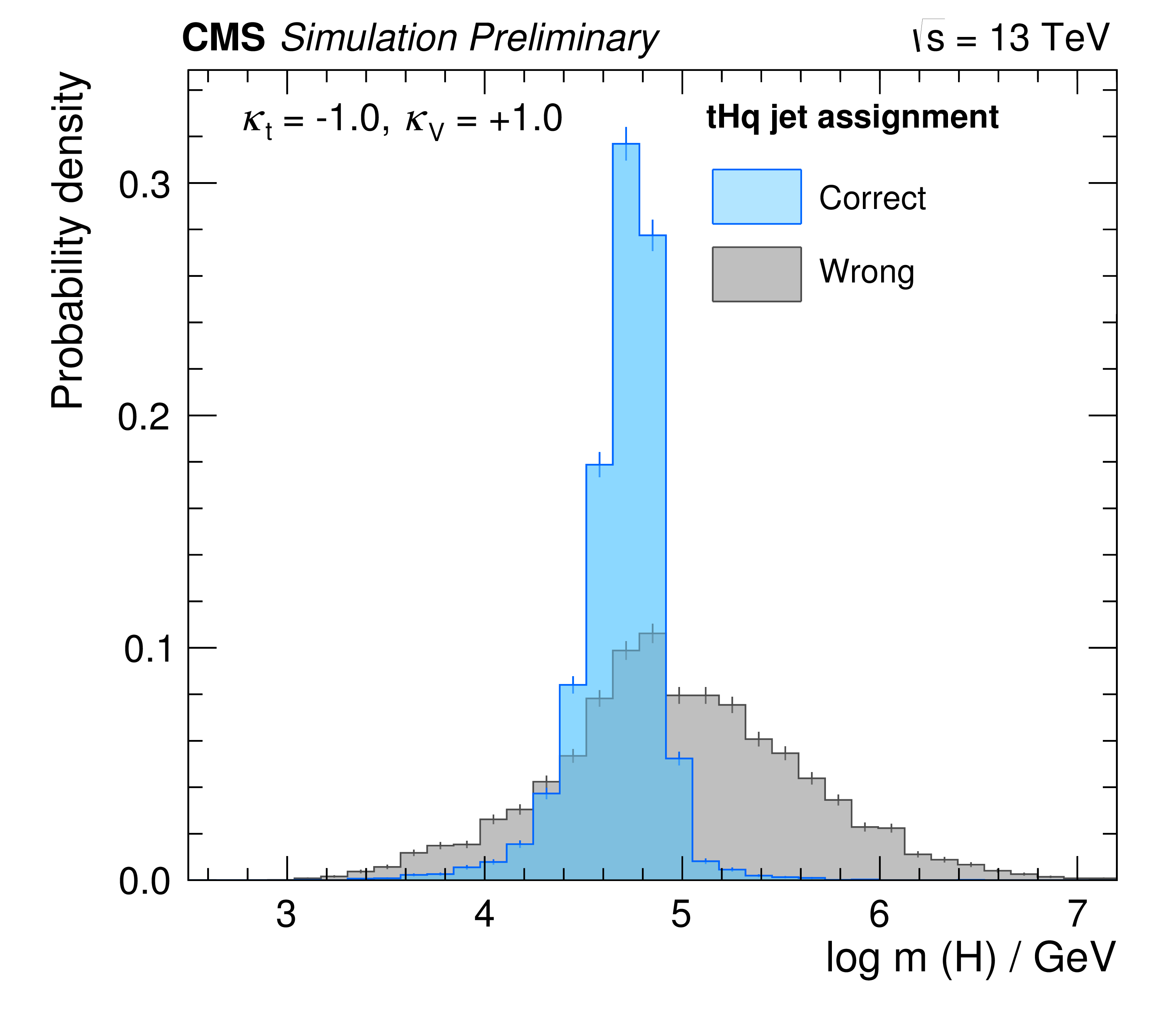
Additional Figure 3:
The most discriminating variable in the tHq reconstruction BDT: The mass of the reconstructed Higss boson candidate for correct and wrong jet-quark assignments. The distributions are normalized to unit area. |
png pdf |
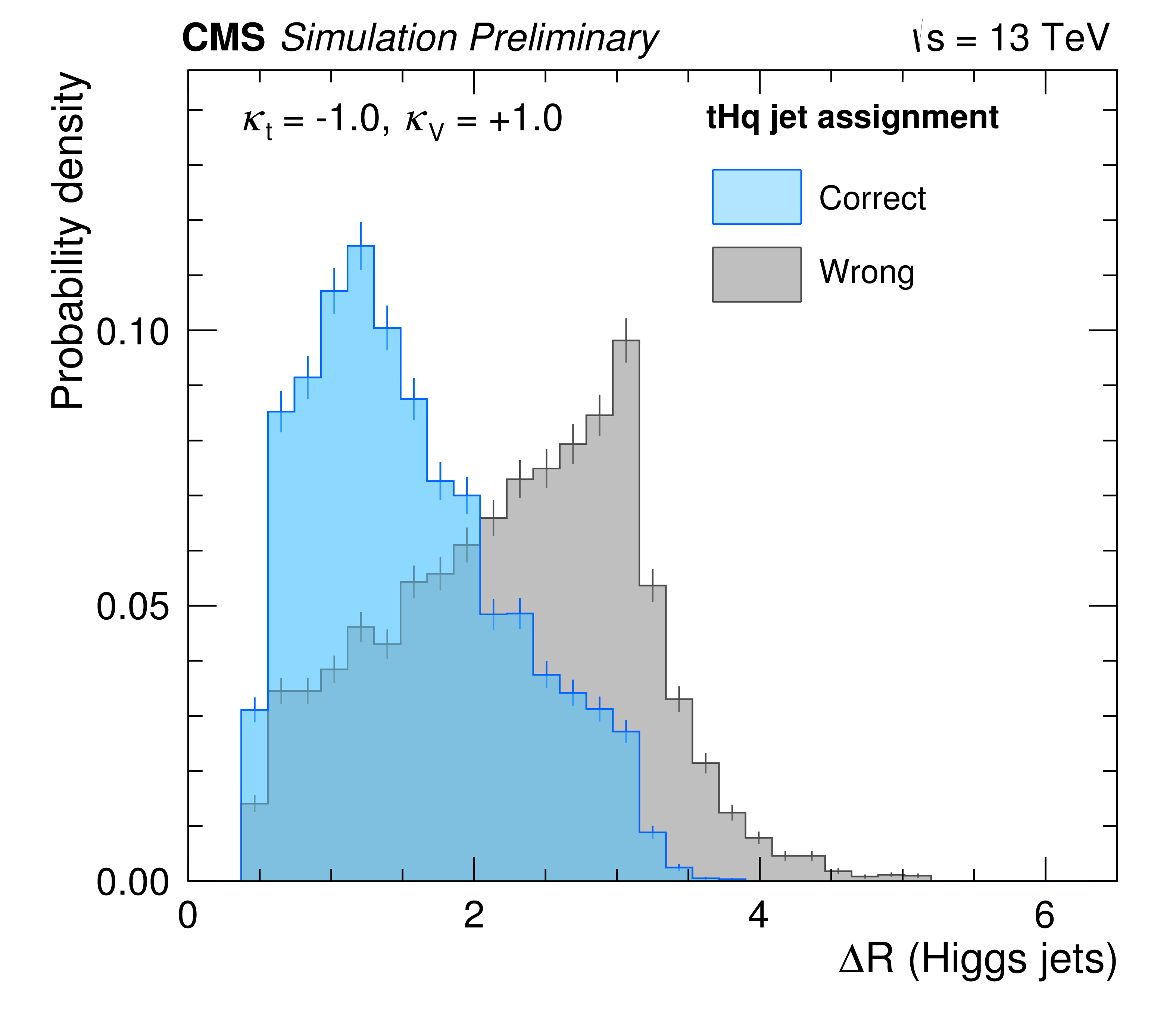
Additional Figure 4:
Input variable of the tHq reconstruction BDT: The $\Delta \text {R}$ between the two jets assigned to the two quarks from the Higgs-boson decay for correct and wrong jet-quark assignments. The distributions are normalized to unit area. |
png pdf |
Additional Figure 5:
Input variable of the tHq reconstruction BDT: The percentage of the total transverse momenta (jets, leptons, and missing transverse energy) that falls to the jet assigned to the b quark from the top-quark decay, the jets assigned to the two b quarks from the Higgs-boson decay, and the recoil jet for correct and wrong jet-quark assignments. The distributions are normalized to unit area. |
png pdf |
Additional Figure 6:
Response of the tH reconstruction BDT in the 2 tag region for the ITC scenario. |
png pdf |
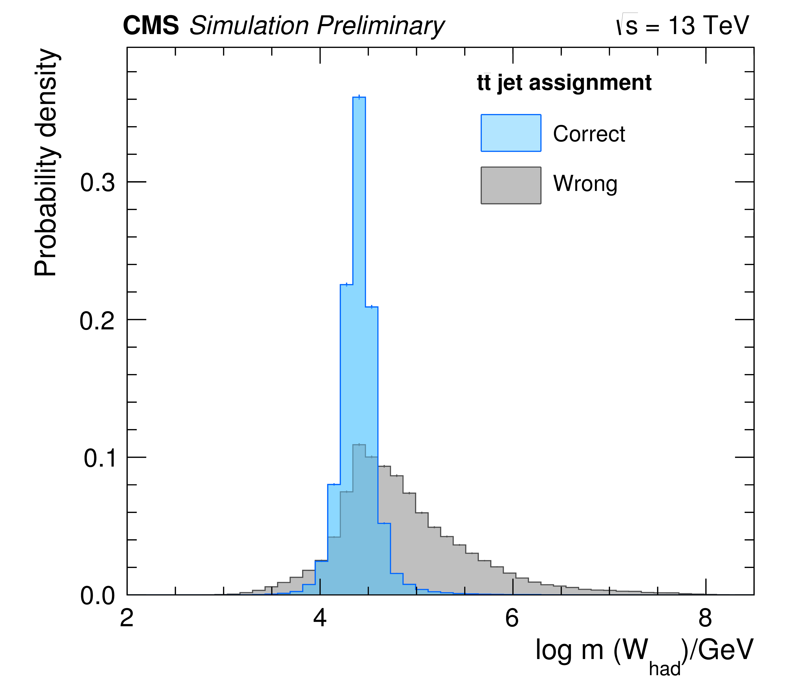
Additional Figure 7:
Input variable of the $\mathrm {t\bar{t}}$ reconstruction BDT: Invariant mass of the two jets assigned to the hadronically decaying W boson for correct and wrong jet-quark assignments. The distributions are normalized to unit area. |
png pdf |
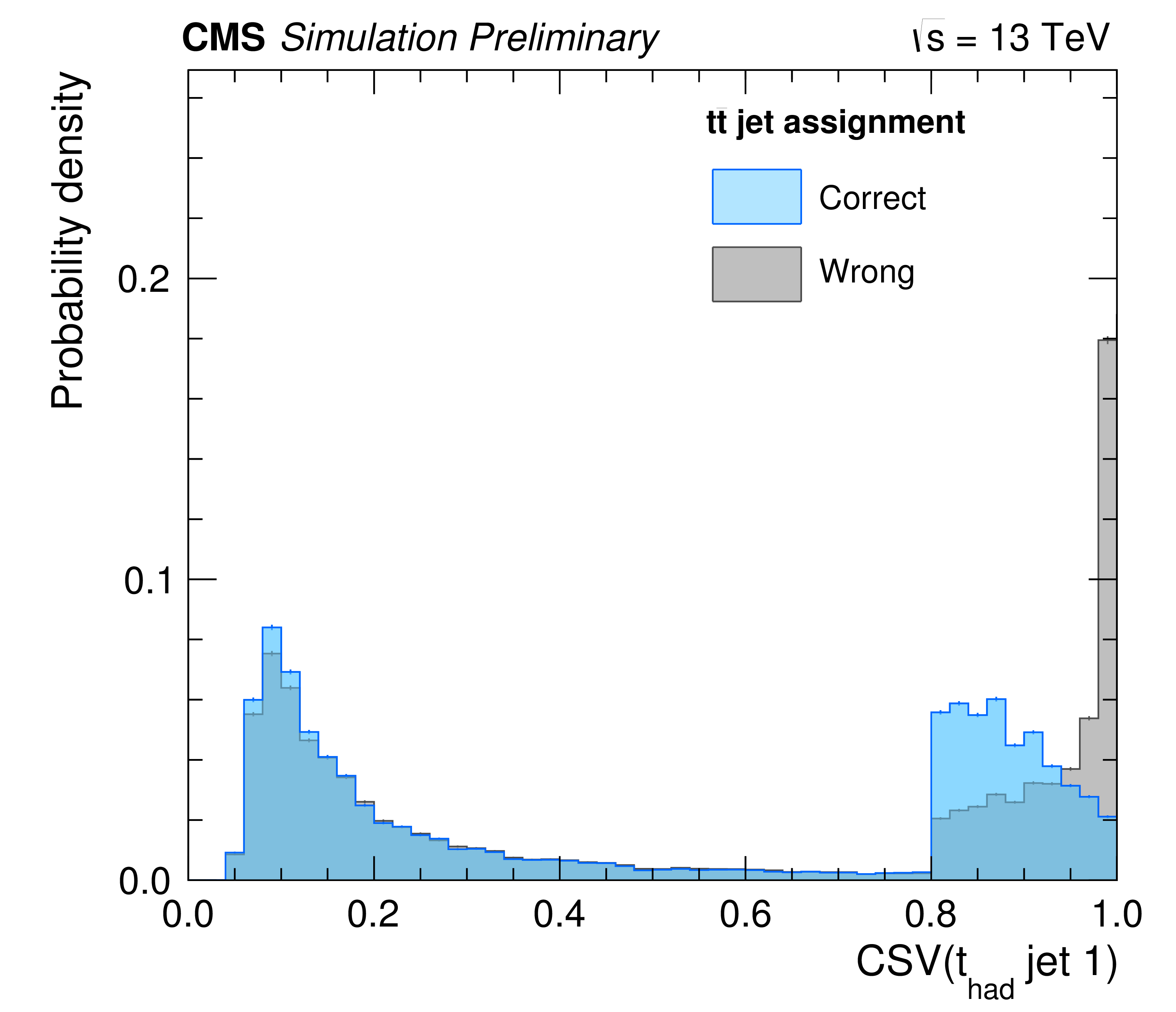
Additional Figure 8:
Input variable of the $\mathrm {t\bar{t}}$ reconstruction BDT: Output of the CSVv2 algorithm for the hardest jet assigned to the hadronically decaying W boson for correct and wrong jet-quark assignments. The distributions are normalized to unit area. |
png pdf |
Additional Figure 9:
Input variable of the $\mathrm {t\bar{t}}$ reconstruction BDT: The $\Delta \text {R}$ between the bjet assigned to the b quark from the reconstructed semileptonically decaying top quark and the leptonically decaying W boson for correct and wrong jet-quark assignments. The distributions are normalized to unit area. |
png pdf |
Additional Figure 10:
Response of the $\mathrm {t\bar{t}}$ reconstruction BDT in the 2 tag region. |
png pdf |
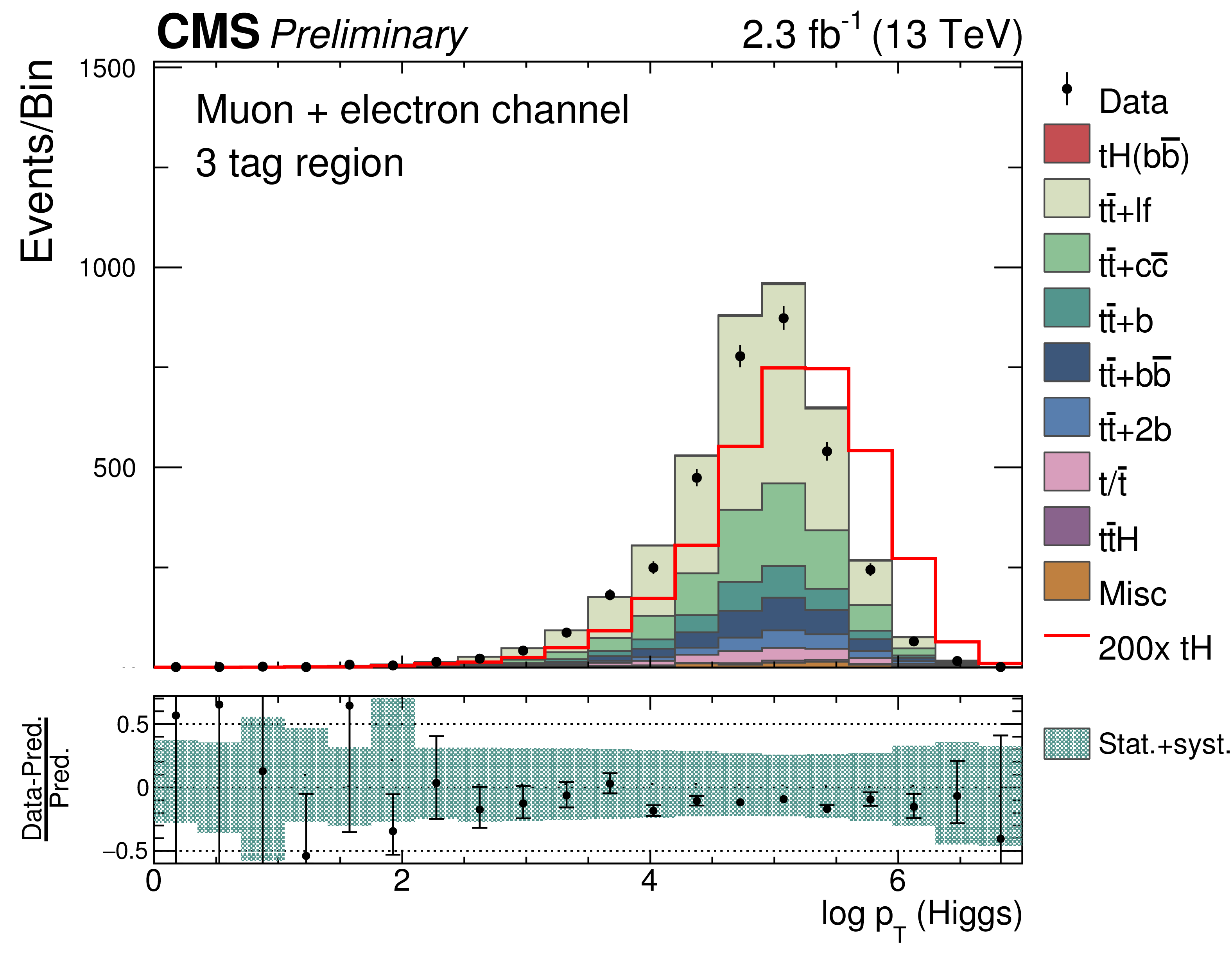
Additional Figure 11:
Input variable of the classification BDT: Logarithm of the transverse momentum of the reconstructed Higgs boson. The distributions are shown in the 3 tag region and are normalized to their predicted yields. |

png pdf |
Additional Figure 12:
Input variable of the classification BDT: Logarithm of the invariant mass of the reconstructed hadronically decaying top quark. The distributions are shown in the 3 tag region and are normalized to their predicted yields. |
png pdf |
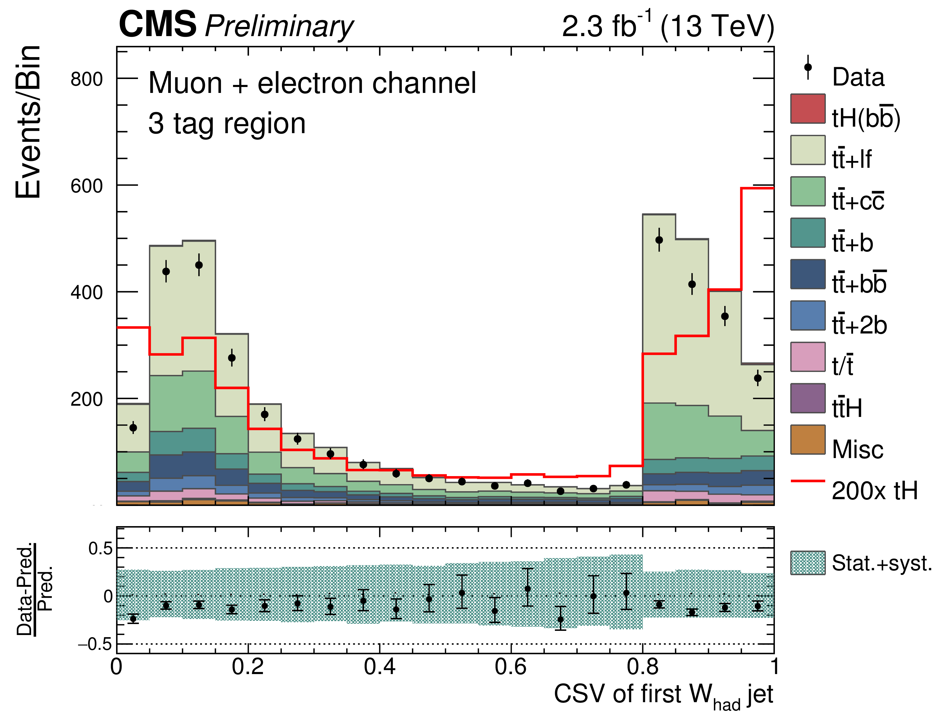
Additional Figure 13:
Input variable of the classification BDT: CSV output of the jet assigned to the first quark of the hadronically decaying W boson. The distributions are shown in the 3 tag region and are normalized to their predicted yields. |
png pdf |
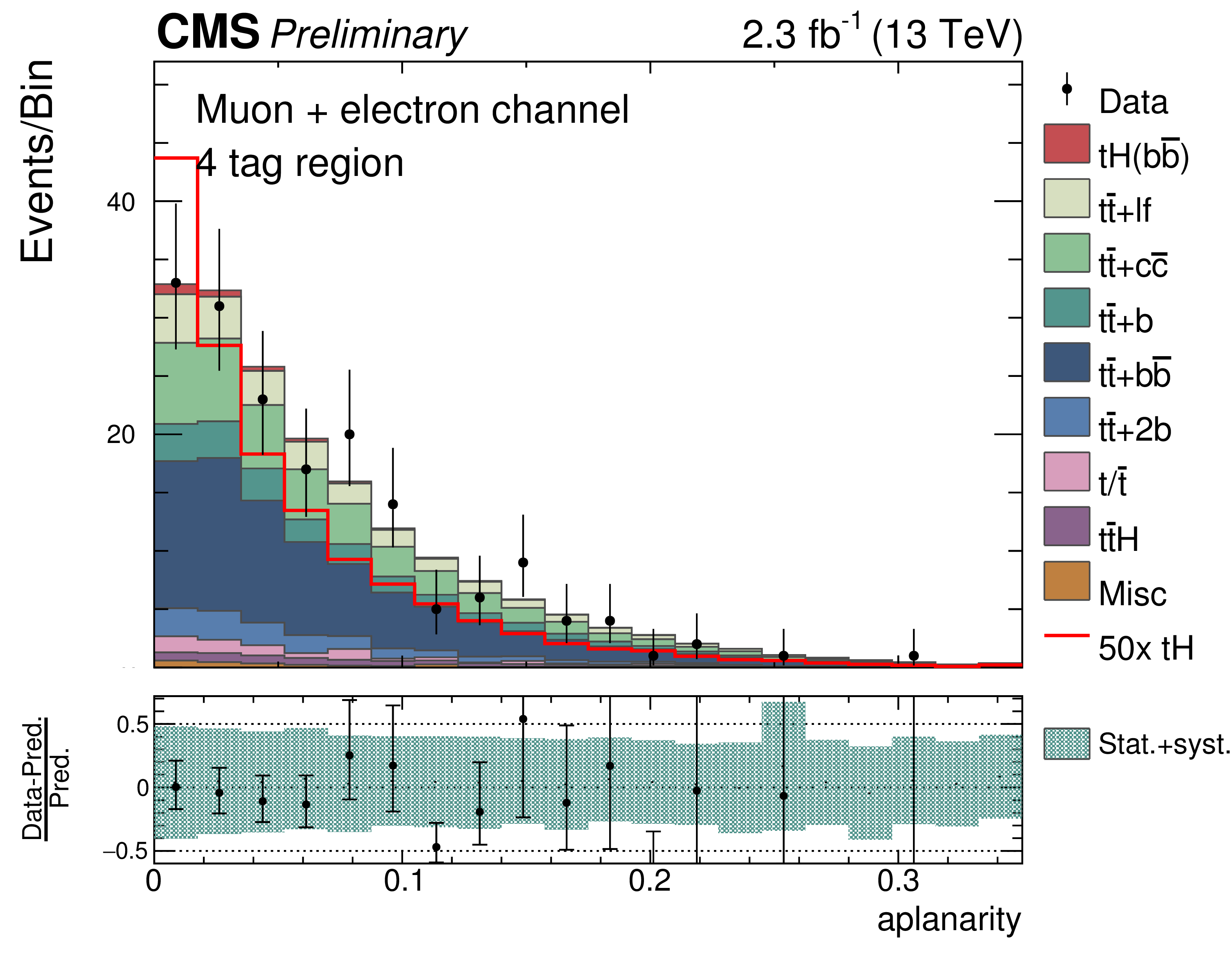
Additional Figure 14:
Input variable of the classification BDT: Aplanarity of the event. The distributions are shown in the 4 tag region and are normalized to their predicted yields. |
png pdf |
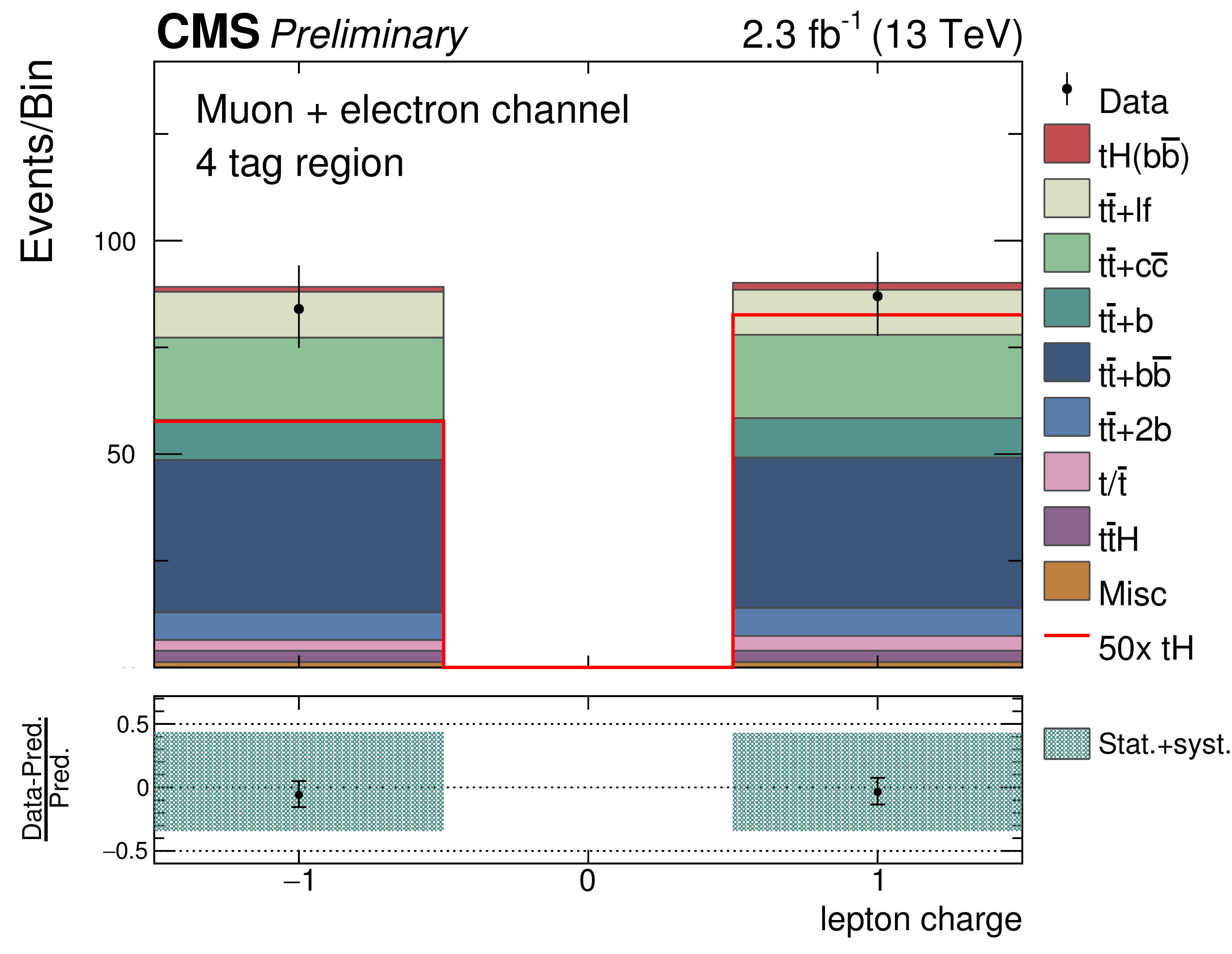
Additional Figure 15:
Input variable of the classification BDT: Sign of the charge of the charged lepton in the event. The distributions are shown in the 4 tag region and are normalized to their predicted yields. |
png pdf |
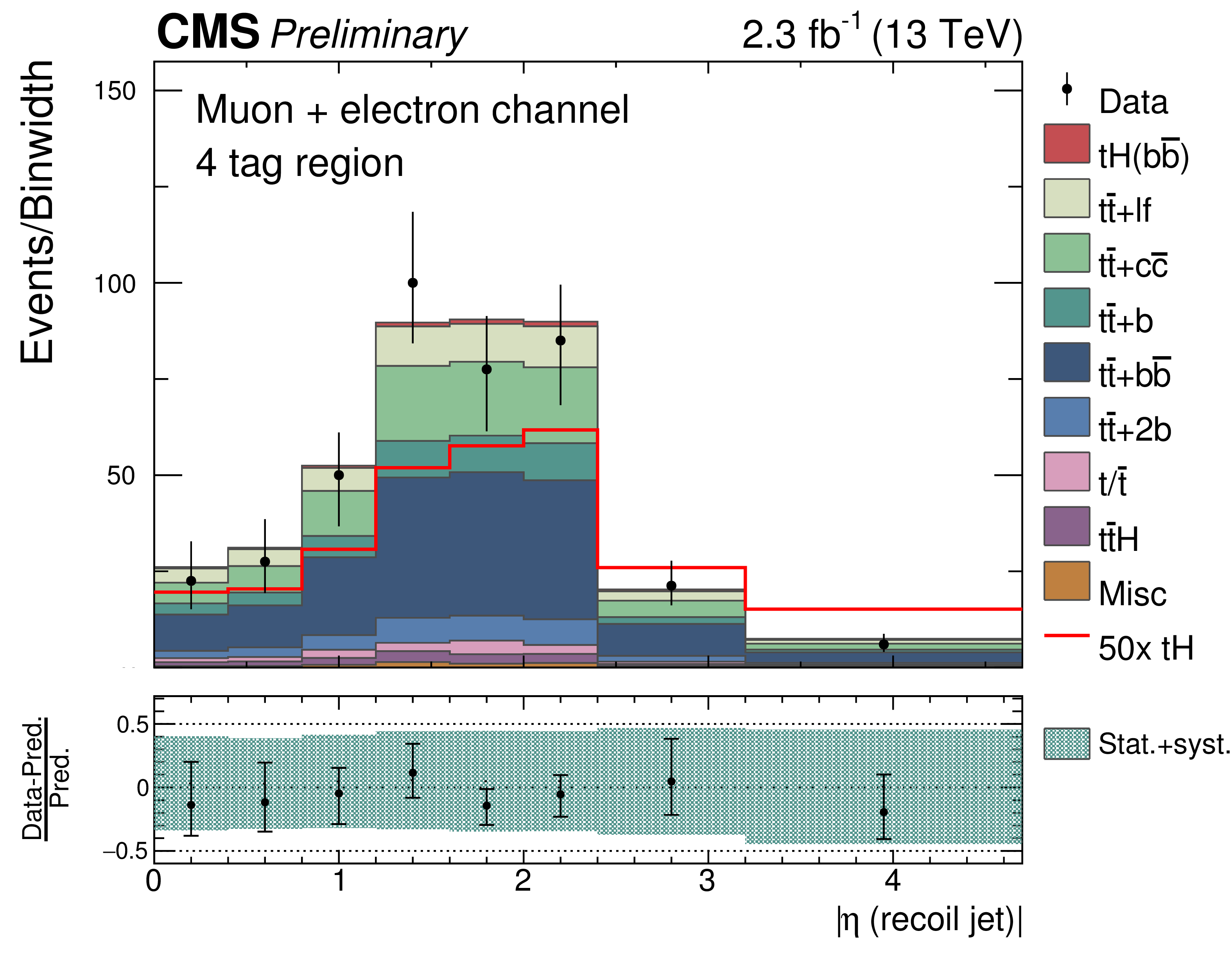
Additional Figure 16:
Input variable of the classification BDT: Absolute pseudorapidity of the reconstructed recoil jet. The distribution is shown in the 4 tag region and is normalized to their predicted yields. |
| References | ||||
| 1 | CMS Collaboration | Observation of a new boson at a mass of 125$ GeV $ with the CMS experiment at the LHC | JHEP 06 (2013) 081 | |
| 2 | ATLAS Collaboration | Observation of a new particle in the search for the Standard Model Higgs boson with the ATLAS detector at the LHC | PLB 716 (2012) 1 | 1207.7214 |
| 3 | S. Biswas, E. Gabrielli, and B. Mele | Single top and Higgs associated production as a probe of the Htt coupling sign at the LHC | JHEP 01 (2013) 088 | 1211.0499 |
| 4 | B. Hespel, F. Maltoni, and E. Vryonidou | Higgs and Z boson associated production via gluon fusion in the SM and the 2HDM | JHEP 06 (2015) 065 | 1503.01656 |
| 5 | ATLAS Collaboration | Measurements of Higgs boson production and couplings in diboson final states with the ATLAS detector at the LHC | PLB 726 (2013) 88 | |
| 6 | CMS Collaboration | Precise determination of the mass of the Higgs boson and tests of compatibility of its couplings with the standard model predictions using proton collisions at 7 and 8 $ \,\text {TeV} $ | EPJC 75 (2015), no. 5, 212 | CMS-HIG-14-009 1412.8662 |
| 7 | ATLAS, CMS Collaboration | Measurements of the Higgs boson production and decay rates and constraints on its couplings from a combined ATLAS and CMS analysis of the LHC $ pp $ collision data at $ \sqrt{s}= $ 7 and 8 TeV | Submitted to JHEP | 1606.02266 |
| 8 | J. Ellis and T. You | Updated Global Analysis of Higgs Couplings | JHEP 06 (2013) 103 | 1303.3879 |
| 9 | G. Bordes and B. van Eijk | On the associate production of a neutral intermediate mass Higgs boson with a single top quark at the LHC and SSC | PLB 299 (1993) 315 | |
| 10 | T. M. P. Tait and C. P. Yuan | Single top quark production as a window to physics beyond the standard model | PRD 63 (2000) 014018 | hep-ph/0007298 |
| 11 | M. Farina et al. | Lifting degeneracies in Higgs couplings using single top production in association with a Higgs boson | JHEP 1305 (2013) 022 | 1211.3736 |
| 12 | F. Demartin, F. Maltoni, K. Mawatari, and M. Zaro | Higgs production in association with a single top quark at the LHC | EPJC 75 (2015), no. 6, 267 | |
| 13 | J. Alwall et al. | The automated computation of tree-level and next-to-leading order differential cross sections, and their matching to parton shower simulations | JHEP 07 (2014) 079 | 1405.0301 |
| 14 | F. Demartin et al. | tWH associated production at the LHC | 1607.05862 | |
| 15 | CMS Collaboration | Search for $ H \to b\bar b $ in association with single top quarks as a test of Higgs couplings | CMS-PAS-HIG-14-015 | CMS-PAS-HIG-14-015 |
| 16 | CMS Collaboration | CMS Luminosity Measurement for the 2015 Data Taking Period | CMS-PAS-LUM-15-001 | CMS-PAS-LUM-15-001 |
| 17 | CMS Collaboration | The CMS experiment at the CERN LHC | JINST 3 (2008) S08004 | CMS-00-001 |
| 18 | NNPDF Collaboration | Parton distributions for the LHC Run II | JHEP 04 (2015) 040 | 1410.8849 |
| 19 | P. Nason | A New Method for Combining NLO QCD with Shower Monte Carlo Algorithms | JHEP 11 (2004) 040 | hep-ph/0409146 |
| 20 | S. Frixione, P. Nason, and C. Oleari | Matching NLO QCD computations with Parton Shower simulations: the POWHEG method | JHEP 11 (2007) 070 | 0709.2092 |
| 21 | S. Alioli, P. Nason, C. Oleari, and E. Re | A general framework for implementing NLO calculations in shower Monte Carlo programs: the POWHEG BOX | JHEP 06 (2010) 043 | 1002.2581 |
| 22 | J. Alwall et al. | The automated computation of tree-level and next-to-leading order differential cross sections, and their matching to parton shower simulations | JHEP 07 (2014) 079 | 1405.0301 |
| 23 | T. Sjostrand, S. Mrenna, and P. Z. Skands | A Brief Introduction to PYTHIA 8.1 | CPC 178 (2008) 852 | 0710.3820 |
| 24 | GEANT4 Collaboration | GEANT4: A Simulation toolkit | NIMA 506 (2003) 250 | |
| 25 | J. Allison et al. | Geant4 developments and applications | IEEE Transactions on Nuclear Science 53 (Feb, 2006) 270 | |
| 26 | CMS Collaboration | Particle-Flow Event Reconstruction in CMS and Performance for Jets, Taus, and $ \ETslash $ | CDS | |
| 27 | CMS Collaboration | Particle-flow commissioning with muons and electrons from J/Psi and W events at 7 TeV | CDS | |
| 28 | M. Cacciari, G. P. Salam, and G. Soyez | The anti-$ k_t $ jet clustering algorithm | JHEP 04 (2008) 063 | 0802.1189 |
| 29 | CMS Collaboration | Jet energy scale and resolution in the CMS experiment in pp collisions at 8 TeV | Submitted to JINST | CMS-JME-13-004 1607.03663 |
| 30 | CMS Collaboration | Identification of b quark jets at the CMS Experiment in the LHC Run 2 | CMS-PAS-BTV-15-001 | CMS-PAS-BTV-15-001 |
| 31 | CMS Collaboration | Performance of the CMS missing transverse momentum reconstruction in pp data at $ \sqrt{s} $ = 8 TeV | JINST 10 (2015), no. 02, P02006 | CMS-JME-13-003 1411.0511 |
| 32 | A. Hoecker et al. | TMVA - Toolkit for Multivariate Data Analysis | physics/0703039 | |
| 33 | CMS Collaboration | Determination of jet energy calibration and transverse momentum resolution in CMS | JINST 6 (2011), no. 11, P11002 | |
| 34 | CMS Collaboration | Search for $ \mathrm{t\overline{t}H} $ production in the $ \mathrm{H}\rightarrow \mathrm{b\overline{b}} $ decay channel with $ \sqrt{s}=13 \mathrm{TeV} $ pp collisions at the CMS experiment | CMS-PAS-HIG-16-004 | CMS-PAS-HIG-16-004 |
| 35 | G. Cowan, K. Cranmer, E. Gross, and O. Vitells | Asymptotic formulae for likelihood-based tests of new physics | EPJC 71 (2011) 1554, [Erratum: Eur. Phys. J.C73,2501(2013)] | 1007.1727 |
|
|
Compact Muon Solenoid LHC, CERN |
|

|

|

|

|

|