

Compact Muon Solenoid
LHC, CERN
| CMS-PAS-SMP-22-008 | ||
| Measurement of W$^{\pm}$W$^{\pm} $ scattering in proton-proton collisions at $ \sqrt{s} =$ 13 TeV in final states with one tau lepton | ||
| CMS Collaboration | ||
| 21 August 2023 | ||
| Abstract: A measurement of the cross section for the scattering of same-sign W bosons is presented. This is the first study of a vector boson scattering process in the decay channel with a tau lepton ($ \tau $). The analysis is performed with proton-proton collision data collected by the CMS detector at the LHC at a center-of-mass energy of 13 TeV, corresponding to an integrated luminosity of 138 fb$ ^{-1} $. Events are selected with the requirement of one $ \tau $, one light lepton ($ e $ or $ \mu $), missing transverse momentum, and two jets with large pseudorapidity separation and large dijet invariant mass. The measured electroweak same-sign WW scattering cross section, extracted with the amplitude for the QCD-associated diboson production fixed to the standard model value, is 1.44 $ ^{+0.63}_{-0.56} $ times the standard model prediction. The observed (expected) signal significance is 2.7 (1.9) standard deviations. A measurement of the combined electroweak and QCD-associated same-sign diboson production yields an observed (expected) significance of 2.9 (2.0) standard deviations. | ||
| Links: CDS record (PDF) ; CADI line (restricted) ; | ||
| Figures & Tables | Summary | Additional Figures & Tables | References | CMS Publications |
|---|
| Figures | |
png pdf |
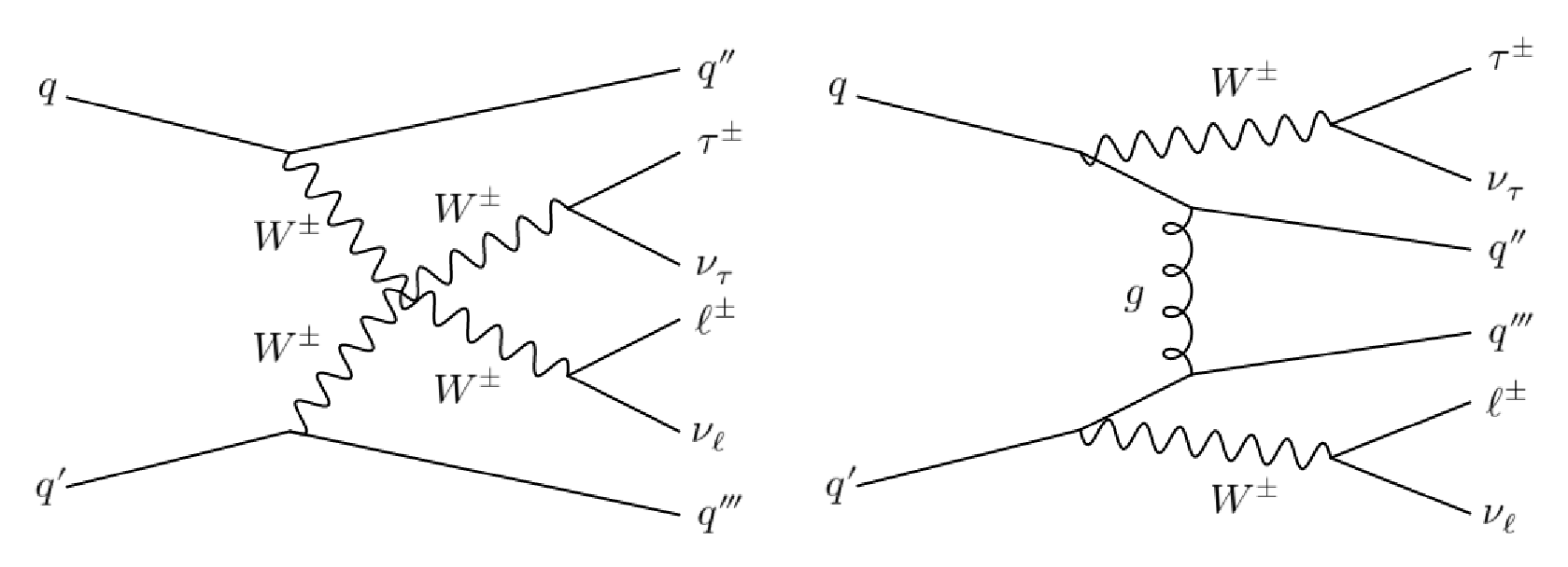
Figure 1:
Representative Born level Feynman diagrams contributing to the process $ pp \rightarrow \tau^{\pm} \nu_{\tau} \ell^{\pm} \nu_{\ell} jj $, $ \ell=$ e, $ \mu $, with $ \mathcal{O}(\alpha^6) $ (left) and $ \mathcal{O}(\alpha_{s}^{2}\alpha^4) $ (right) couplings. |

png pdf |
Figure 1-a:
Representative Born level Feynman diagrams contributing to the process $ pp \rightarrow \tau^{\pm} \nu_{\tau} \ell^{\pm} \nu_{\ell} jj $, $ \ell=$ e, $ \mu $, with $ \mathcal{O}(\alpha^6) $ (left) and $ \mathcal{O}(\alpha_{s}^{2}\alpha^4) $ (right) couplings. |

png pdf |
Figure 1-b:
Representative Born level Feynman diagrams contributing to the process $ pp \rightarrow \tau^{\pm} \nu_{\tau} \ell^{\pm} \nu_{\ell} jj $, $ \ell=$ e, $ \mu $, with $ \mathcal{O}(\alpha^6) $ (left) and $ \mathcal{O}(\alpha_{s}^{2}\alpha^4) $ (right) couplings. |

png pdf |
Figure 2:
Distributions in the invariant mass of the di-jet system for the data and the pre-fit background prediction for the (left) e+$\tau_\mathrm{h} $ and (right) $\mu$+$\tau_\mathrm{h} $ nonprompt CRs. The overflow count is included in the last bin. The solid red line shows the expectation for the EW ssWW signal. |

png pdf |
Figure 2-a:
Distributions in the invariant mass of the di-jet system for the data and the pre-fit background prediction for the (left) e+$\tau_\mathrm{h} $ and (right) $\mu$+$\tau_\mathrm{h} $ nonprompt CRs. The overflow count is included in the last bin. The solid red line shows the expectation for the EW ssWW signal. |

png pdf |
Figure 2-b:
Distributions in the invariant mass of the di-jet system for the data and the pre-fit background prediction for the (left) e+$\tau_\mathrm{h} $ and (right) $\mu$+$\tau_\mathrm{h} $ nonprompt CRs. The overflow count is included in the last bin. The solid red line shows the expectation for the EW ssWW signal. |
png pdf |
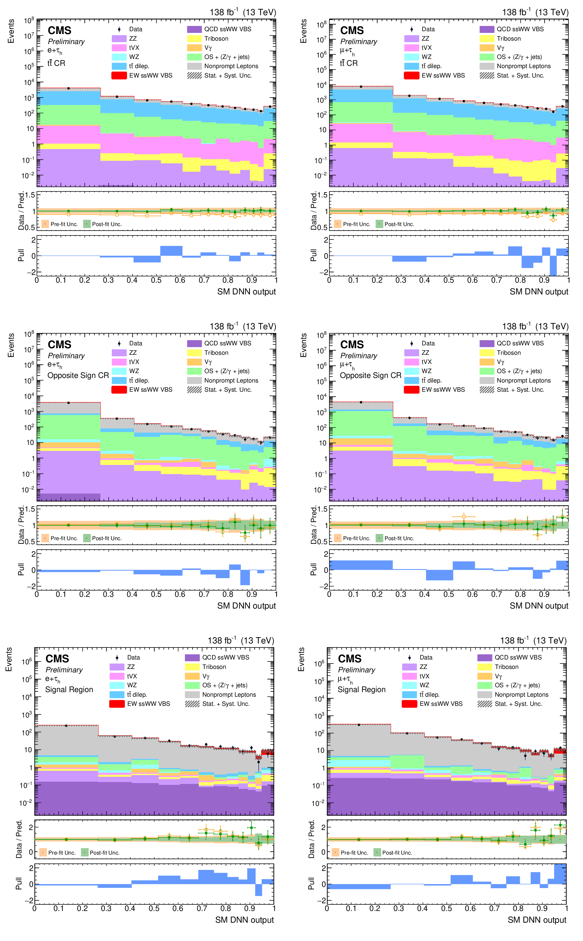
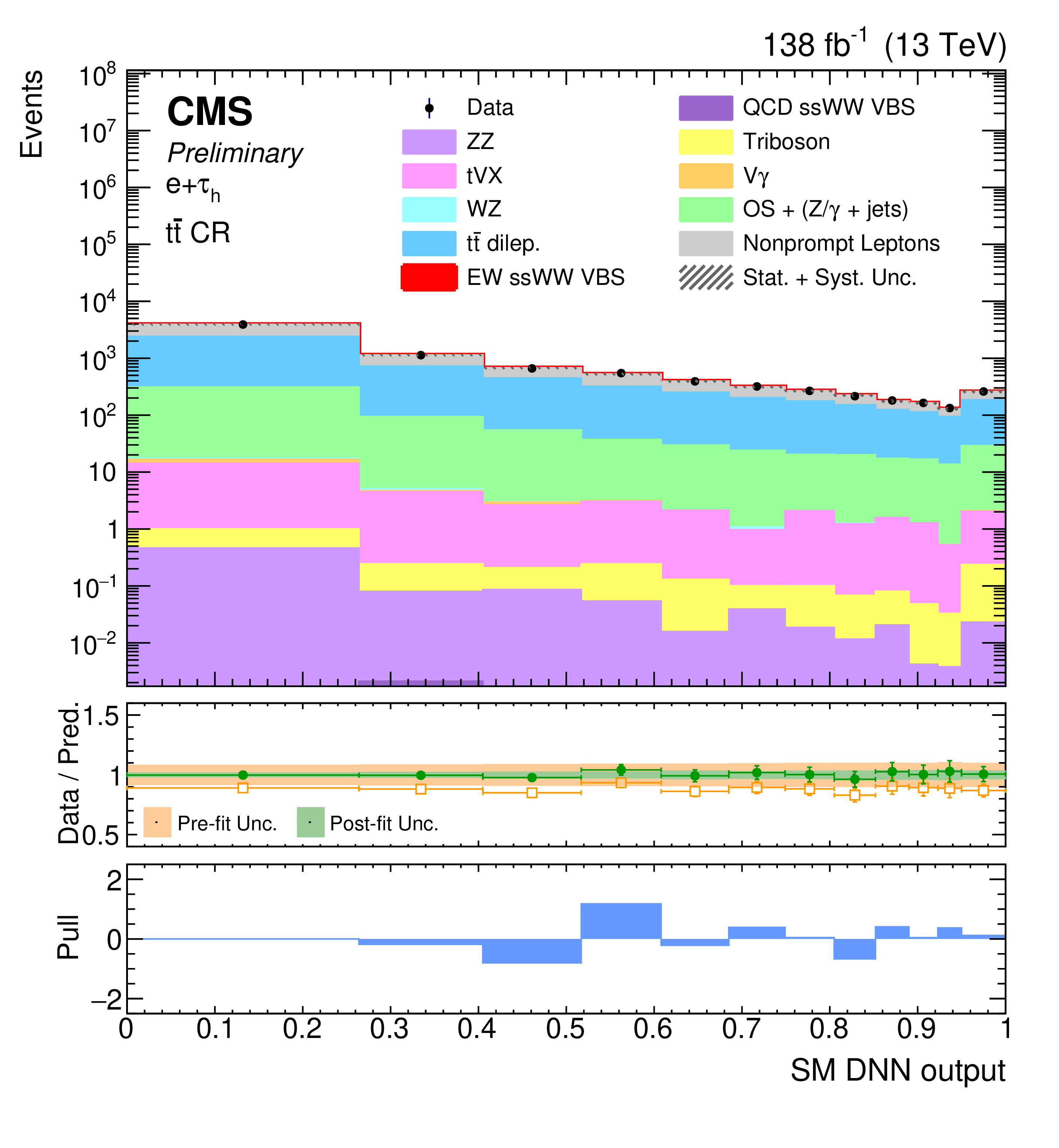
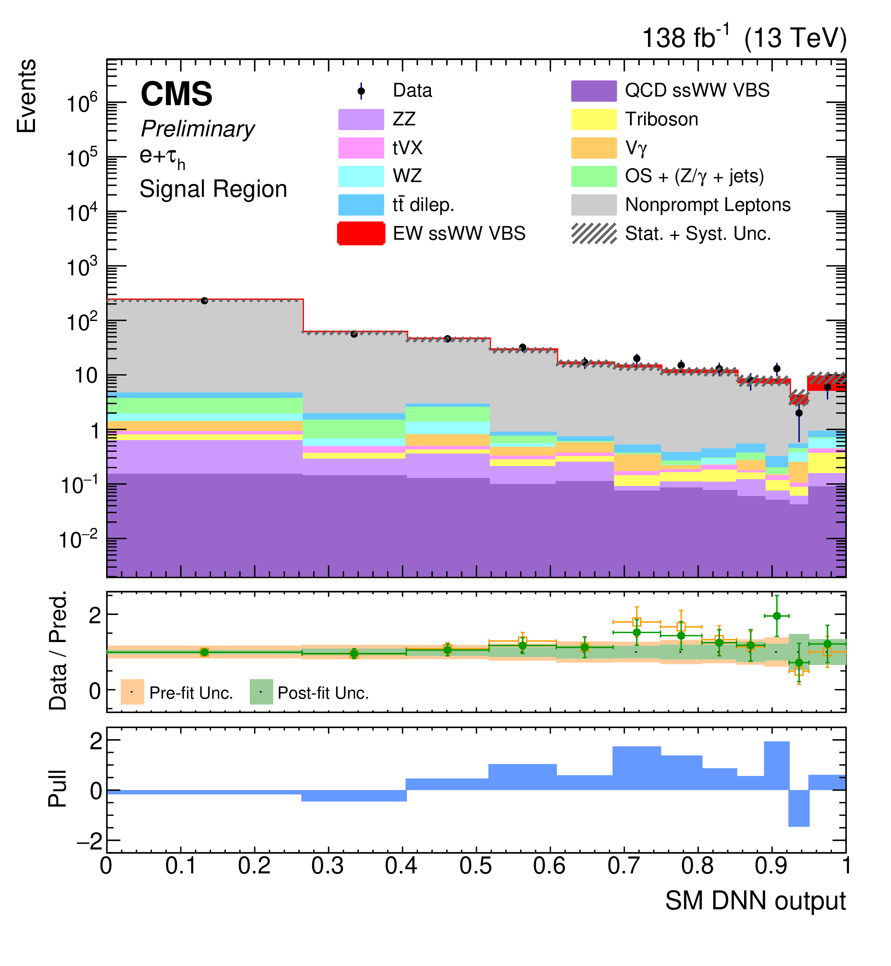
Figure 3:
Distribution of DNN output for the e+$\tau_\mathrm{h} $ (left) and $\mu$+$\tau_\mathrm{h} $ (right) channels for the full data sample, in the $ \mathrm{t} \overline{\mathrm{t}} $ CR (upper), OS CR (middle), and SR (lower) rows. Data points are overlaid on the post-fit background (stacked histograms). The overflow is included in the last bin. The middle panels show ratios of the data to the pre-fit background prediction and post-fit background yield in yellow and green, respectively. The yellow (green) bands in the middle panels indicate the systematic component of the pre-fit (post-fit) uncertainty. The lower panels show the distributions of the pulls, defined in the text. |
png pdf |
Figure 3-a:
Distribution of DNN output for the e+$\tau_\mathrm{h} $ (left) and $\mu$+$\tau_\mathrm{h} $ (right) channels for the full data sample, in the $ \mathrm{t} \overline{\mathrm{t}} $ CR (upper), OS CR (middle), and SR (lower) rows. Data points are overlaid on the post-fit background (stacked histograms). The overflow is included in the last bin. The middle panels show ratios of the data to the pre-fit background prediction and post-fit background yield in yellow and green, respectively. The yellow (green) bands in the middle panels indicate the systematic component of the pre-fit (post-fit) uncertainty. The lower panels show the distributions of the pulls, defined in the text. |

png pdf |
Figure 3-b:
Distribution of DNN output for the e+$\tau_\mathrm{h} $ (left) and $\mu$+$\tau_\mathrm{h} $ (right) channels for the full data sample, in the $ \mathrm{t} \overline{\mathrm{t}} $ CR (upper), OS CR (middle), and SR (lower) rows. Data points are overlaid on the post-fit background (stacked histograms). The overflow is included in the last bin. The middle panels show ratios of the data to the pre-fit background prediction and post-fit background yield in yellow and green, respectively. The yellow (green) bands in the middle panels indicate the systematic component of the pre-fit (post-fit) uncertainty. The lower panels show the distributions of the pulls, defined in the text. |

png pdf |
Figure 3-c:
Distribution of DNN output for the e+$\tau_\mathrm{h} $ (left) and $\mu$+$\tau_\mathrm{h} $ (right) channels for the full data sample, in the $ \mathrm{t} \overline{\mathrm{t}} $ CR (upper), OS CR (middle), and SR (lower) rows. Data points are overlaid on the post-fit background (stacked histograms). The overflow is included in the last bin. The middle panels show ratios of the data to the pre-fit background prediction and post-fit background yield in yellow and green, respectively. The yellow (green) bands in the middle panels indicate the systematic component of the pre-fit (post-fit) uncertainty. The lower panels show the distributions of the pulls, defined in the text. |

png pdf |
Figure 3-d:
Distribution of DNN output for the e+$\tau_\mathrm{h} $ (left) and $\mu$+$\tau_\mathrm{h} $ (right) channels for the full data sample, in the $ \mathrm{t} \overline{\mathrm{t}} $ CR (upper), OS CR (middle), and SR (lower) rows. Data points are overlaid on the post-fit background (stacked histograms). The overflow is included in the last bin. The middle panels show ratios of the data to the pre-fit background prediction and post-fit background yield in yellow and green, respectively. The yellow (green) bands in the middle panels indicate the systematic component of the pre-fit (post-fit) uncertainty. The lower panels show the distributions of the pulls, defined in the text. |
png pdf |
Figure 3-e:
Distribution of DNN output for the e+$\tau_\mathrm{h} $ (left) and $\mu$+$\tau_\mathrm{h} $ (right) channels for the full data sample, in the $ \mathrm{t} \overline{\mathrm{t}} $ CR (upper), OS CR (middle), and SR (lower) rows. Data points are overlaid on the post-fit background (stacked histograms). The overflow is included in the last bin. The middle panels show ratios of the data to the pre-fit background prediction and post-fit background yield in yellow and green, respectively. The yellow (green) bands in the middle panels indicate the systematic component of the pre-fit (post-fit) uncertainty. The lower panels show the distributions of the pulls, defined in the text. |

png pdf |
Figure 3-f:
Distribution of DNN output for the e+$\tau_\mathrm{h} $ (left) and $\mu$+$\tau_\mathrm{h} $ (right) channels for the full data sample, in the $ \mathrm{t} \overline{\mathrm{t}} $ CR (upper), OS CR (middle), and SR (lower) rows. Data points are overlaid on the post-fit background (stacked histograms). The overflow is included in the last bin. The middle panels show ratios of the data to the pre-fit background prediction and post-fit background yield in yellow and green, respectively. The yellow (green) bands in the middle panels indicate the systematic component of the pre-fit (post-fit) uncertainty. The lower panels show the distributions of the pulls, defined in the text. |
| Tables | |
png pdf |
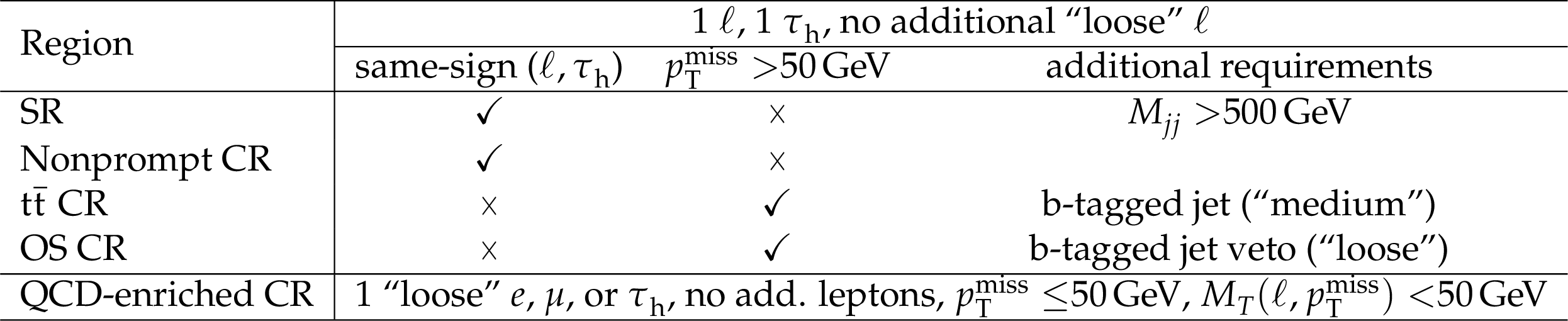
Table 1:
Definition of the SR and four CRs. All regions are disjoint. The SR and three CRs (Nonprompt, $ \mathrm{t} \overline{\mathrm{t}} $, OS) are selected from an inclusive lepton trigger; the QCD enriched CR (last row) is selected from a jet-based trigger. |

png pdf |
Table 2:
The impact of each systematic uncertainty on the signal strength $ \mu $ as extracted from the fit to measure the SM ssWW VBS signal with the DNN output distributions. Upper and lower uncertainties are given for the various sources. |
| Summary |
| Electroweak production of same-sign W boson pairs (ssWW) with a hadronically decaying $ \tau $ ($ \tau_\mathrm{h} $) in the final state is investigated for the first time. The analysis is performed with a sample of proton-proton collisions at $ \sqrt{s} $ = 13 TeV recorded by the CMS experiment at the CERN LHC, corresponding to an integrated luminosity of 138 fb$ ^{-1} $. Deep neural network algorithms are employed to discriminate signal events from the main backgrounds. The measured cross section for electroweak same-sign WW scattering is 1.44 $ ^{+0.63}_{-0.56} $ times the standard model prediction, obtained keeping the QCD-associated diboson production fixed to its standard model prediction. The observed signal significance is 2.7 standard deviations with 1.9 expected. The simultaneous measurement of the electroweak and QCD-associated diboson production is measured with an observed (expected) significance of 2.9 (2.0) standard deviations. |
| Additional Figures | |
png pdf |
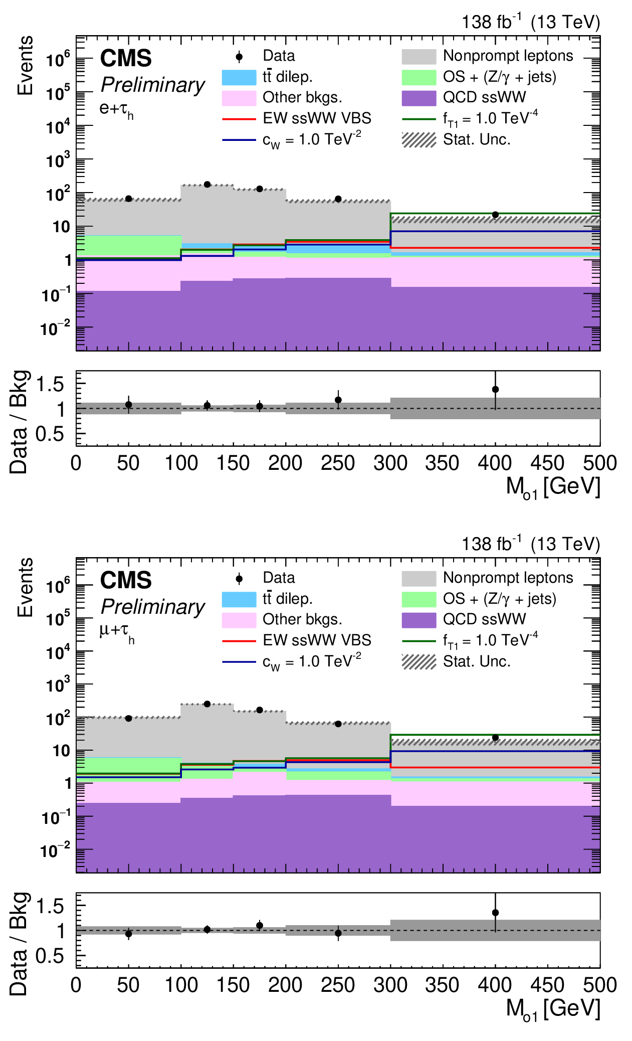
Additional Figure 1:
Distributions of the transverse mass $ M_{o1} $ for the data and the pre-fit background prediction for the (left) $ \mathrm{e}+\tau_\mathrm{h} $ and (right) $ \mu+\tau_\mathrm{h} $ SRs. The overflow count is included in the last bin. The solid red line shows the expectation for the EW ssWW signal, the solid blue line the total one for the $ \mathcal{O}_{W} $ dim-6 operator with $ c_{W}= $ 1 TeV$ ^{-2} $, the solid green line the total one for the $ \mathcal{Q}_{T1} $ dim-8 operator with $ f_{T1}= $ 1 TeV$^{-4} $. For the latter two, the interference with SM and pure EFT contributions are summed together with the SM contribution. |

png pdf |
Additional Figure 1-a:
Distributions of the transverse mass $ M_{o1} $ for the data and the pre-fit background prediction for the (left) $ \mathrm{e}+\tau_\mathrm{h} $ and (right) $ \mu+\tau_\mathrm{h} $ SRs. The overflow count is included in the last bin. The solid red line shows the expectation for the EW ssWW signal, the solid blue line the total one for the $ \mathcal{O}_{W} $ dim-6 operator with $ c_{W}= $ 1 TeV$ ^{-2} $, the solid green line the total one for the $ \mathcal{Q}_{T1} $ dim-8 operator with $ f_{T1}= $ 1 TeV$^{-4} $. For the latter two, the interference with SM and pure EFT contributions are summed together with the SM contribution. |

png pdf |
Additional Figure 1-b:
Distributions of the transverse mass $ M_{o1} $ for the data and the pre-fit background prediction for the (left) $ \mathrm{e}+\tau_\mathrm{h} $ and (right) $ \mu+\tau_\mathrm{h} $ SRs. The overflow count is included in the last bin. The solid red line shows the expectation for the EW ssWW signal, the solid blue line the total one for the $ \mathcal{O}_{W} $ dim-6 operator with $ c_{W}= $ 1 TeV$ ^{-2} $, the solid green line the total one for the $ \mathcal{Q}_{T1} $ dim-8 operator with $ f_{T1}= $ 1 TeV$^{-4} $. For the latter two, the interference with SM and pure EFT contributions are summed together with the SM contribution. |

png pdf |
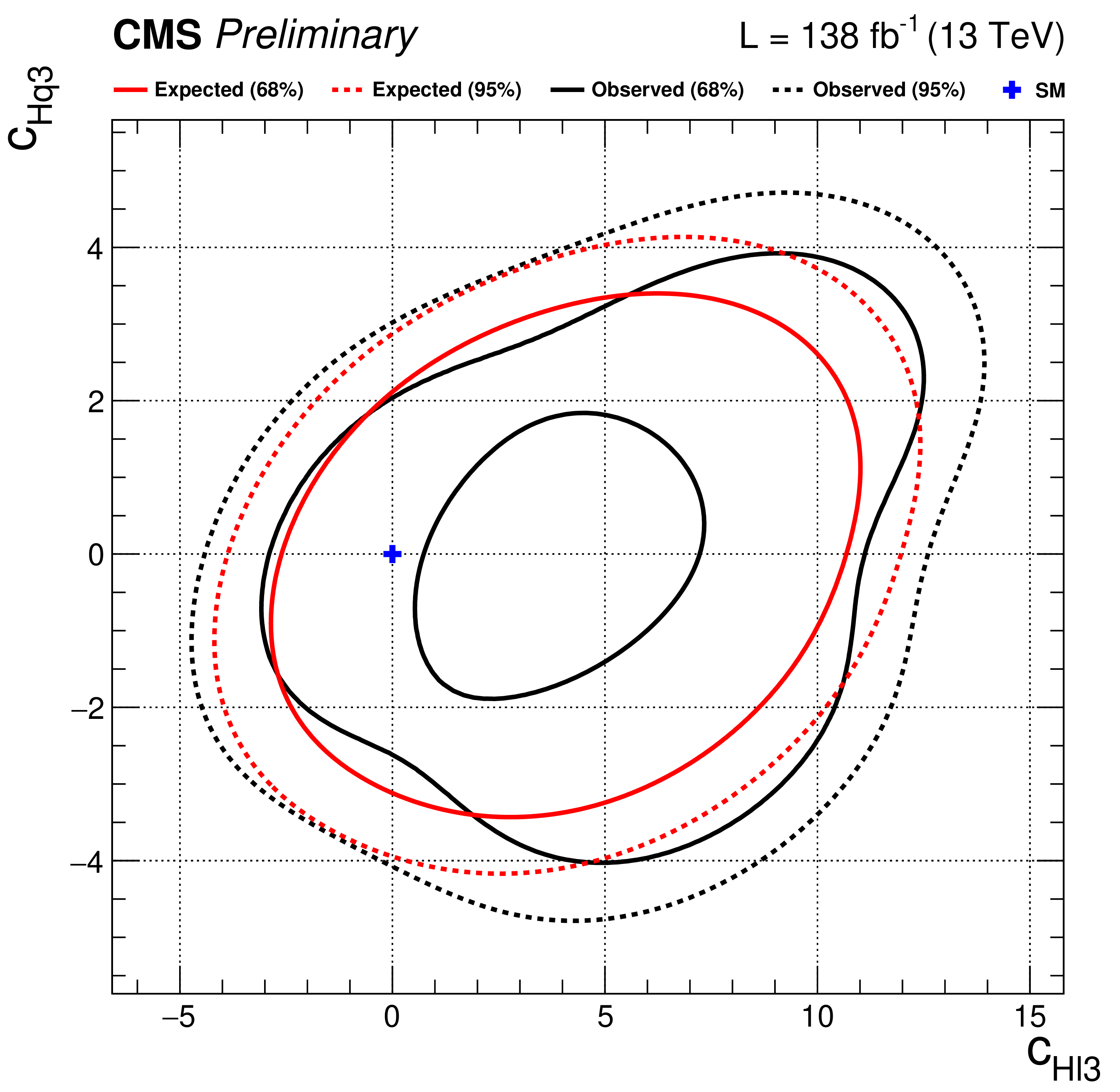
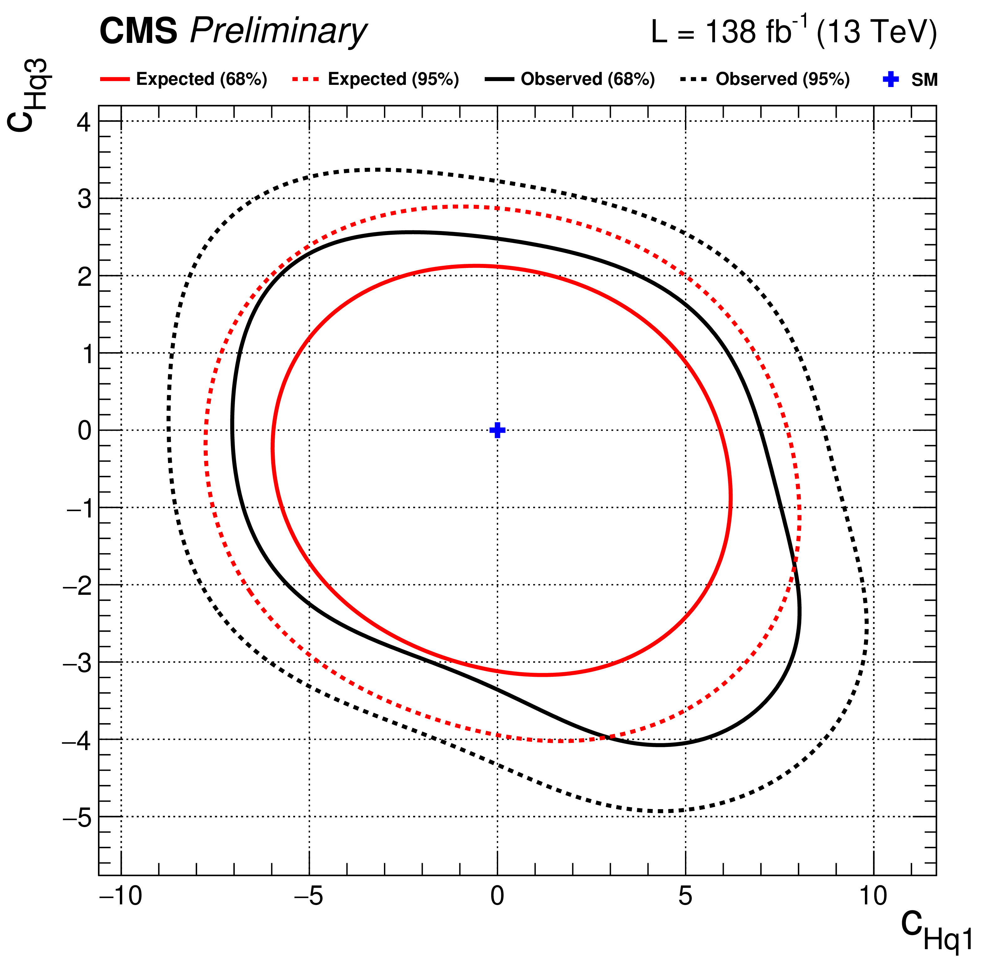
Additional Figure 2:
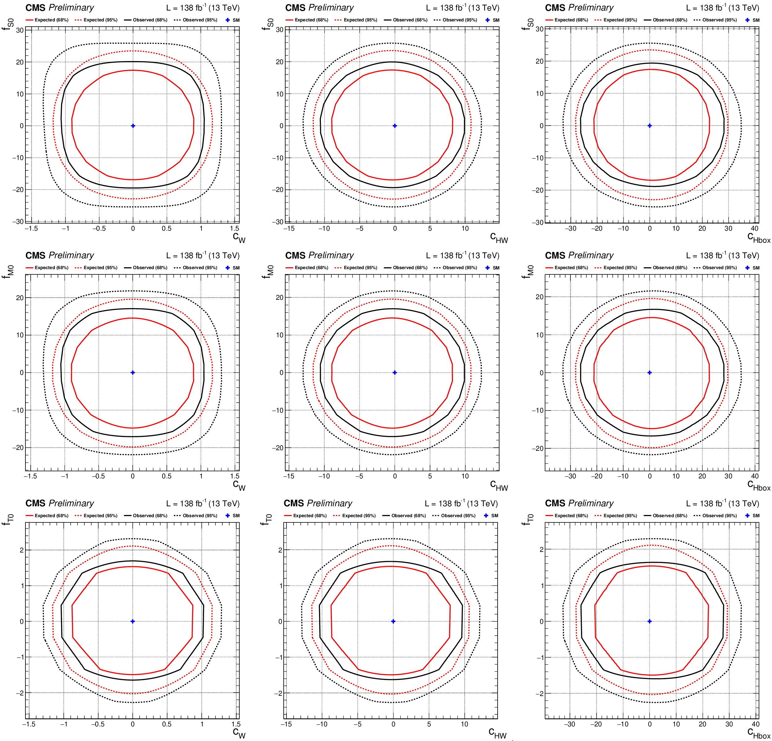
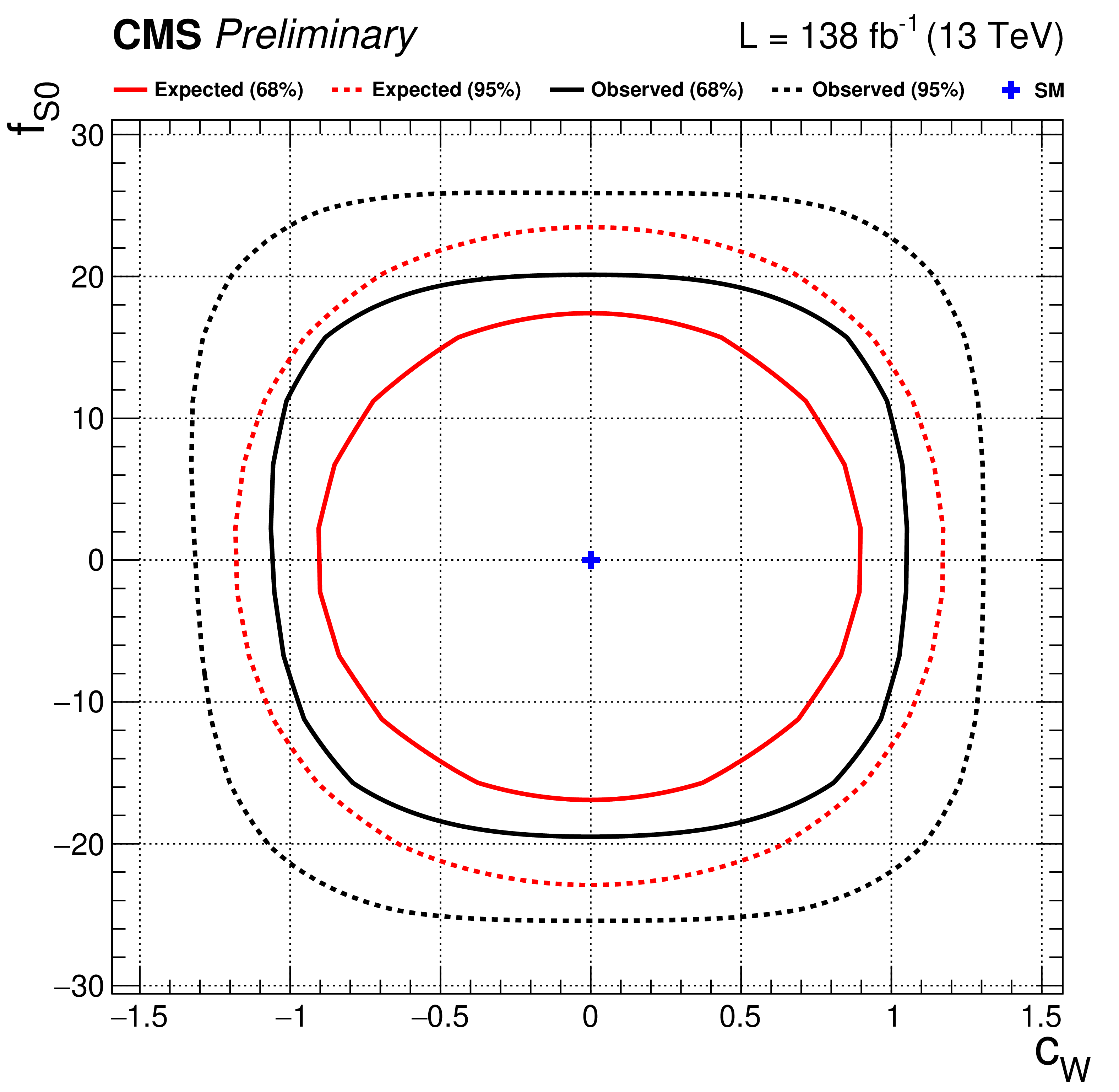
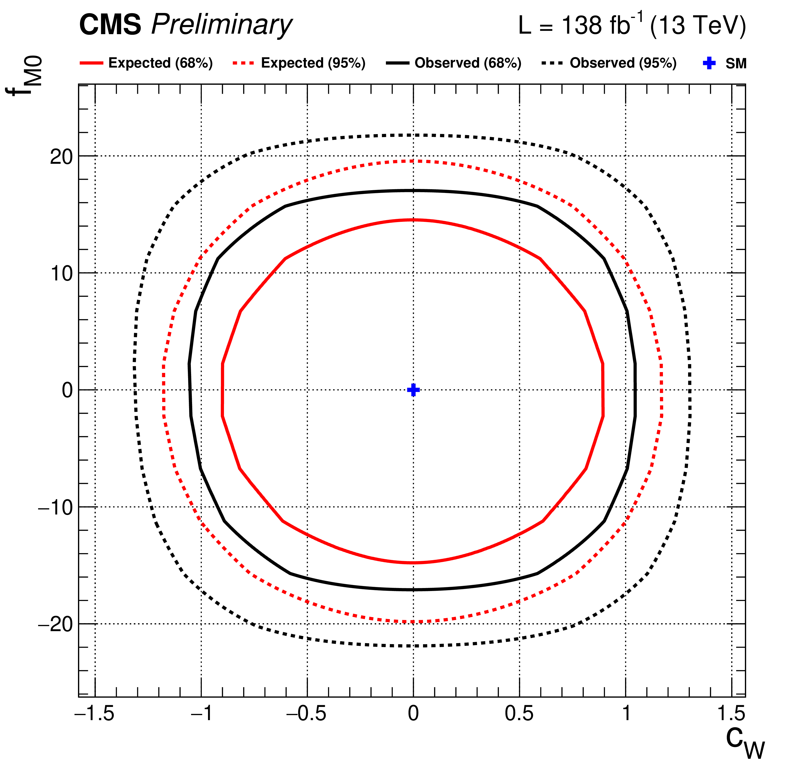
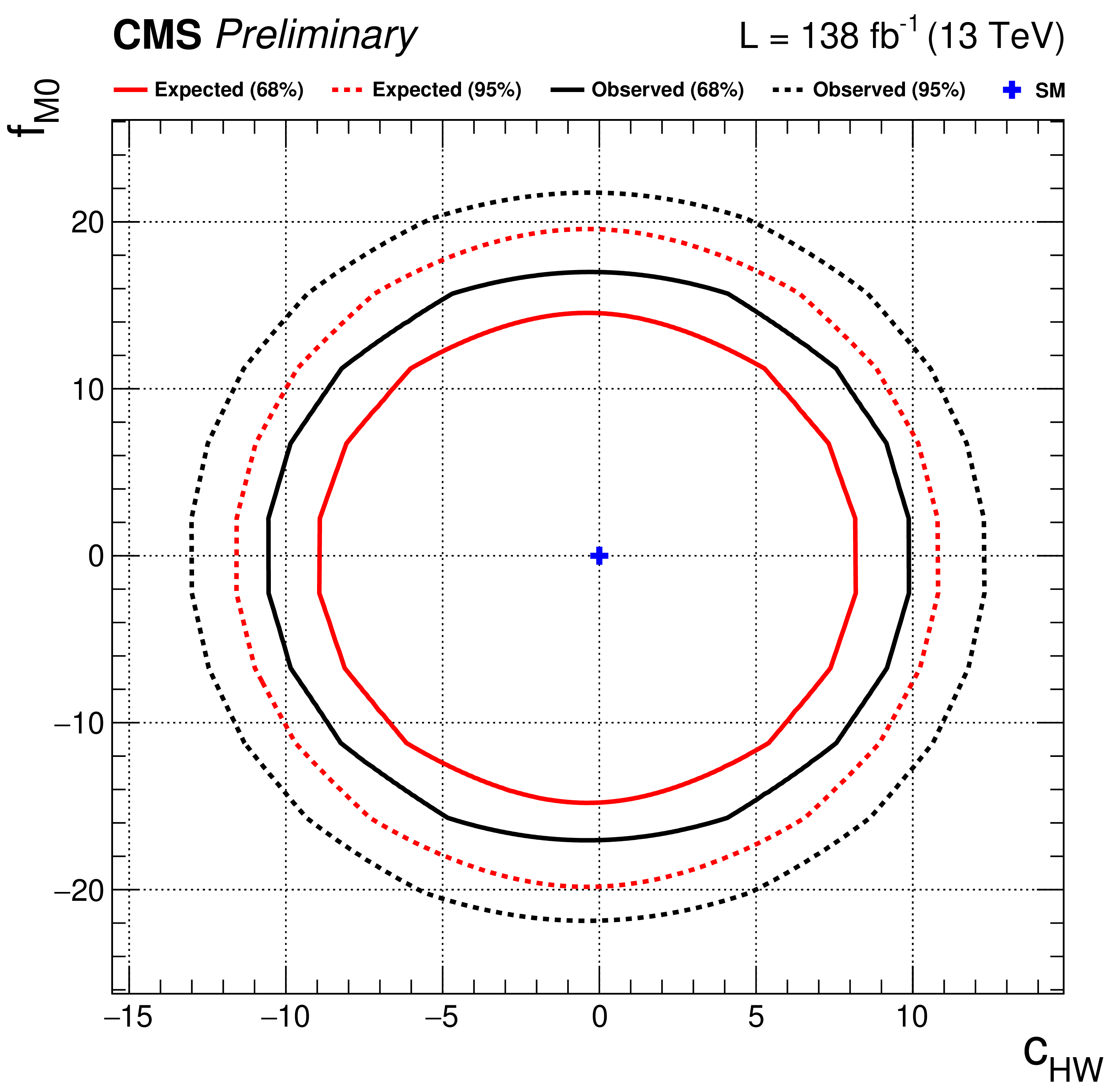
Constraints on pairs of Wilson coefficients, derived from likelihood scans in which all other coefficients are fixed to zero. The pair investigated consists of two EFT operators giving linear and quadratic contributions with similar magnitude and similarly modifying the scattering amplitude by acting on the same type of fields. For the relevant dim-6 bosonic operator pairs, the observed (black) and expected (red) 68% (solid) and 95% (dashed) CL contours for the two-dimensional $ -2\ln\Delta\mathcal{L} $ are reported as functions of the corresponding Wilson coefficient pairs. For these studies, the distributions of the transverse mass $ M_{o1} $ are used in the scans in place of the EFT DNN output distributions. |

png pdf |
Additional Figure 2-a:
Constraints on pairs of Wilson coefficients, derived from likelihood scans in which all other coefficients are fixed to zero. The pair investigated consists of two EFT operators giving linear and quadratic contributions with similar magnitude and similarly modifying the scattering amplitude by acting on the same type of fields. For the relevant dim-6 bosonic operator pairs, the observed (black) and expected (red) 68% (solid) and 95% (dashed) CL contours for the two-dimensional $ -2\ln\Delta\mathcal{L} $ are reported as functions of the corresponding Wilson coefficient pairs. For these studies, the distributions of the transverse mass $ M_{o1} $ are used in the scans in place of the EFT DNN output distributions. |

png pdf |
Additional Figure 2-b:
Constraints on pairs of Wilson coefficients, derived from likelihood scans in which all other coefficients are fixed to zero. The pair investigated consists of two EFT operators giving linear and quadratic contributions with similar magnitude and similarly modifying the scattering amplitude by acting on the same type of fields. For the relevant dim-6 bosonic operator pairs, the observed (black) and expected (red) 68% (solid) and 95% (dashed) CL contours for the two-dimensional $ -2\ln\Delta\mathcal{L} $ are reported as functions of the corresponding Wilson coefficient pairs. For these studies, the distributions of the transverse mass $ M_{o1} $ are used in the scans in place of the EFT DNN output distributions. |

png pdf |
Additional Figure 2-c:
Constraints on pairs of Wilson coefficients, derived from likelihood scans in which all other coefficients are fixed to zero. The pair investigated consists of two EFT operators giving linear and quadratic contributions with similar magnitude and similarly modifying the scattering amplitude by acting on the same type of fields. For the relevant dim-6 bosonic operator pairs, the observed (black) and expected (red) 68% (solid) and 95% (dashed) CL contours for the two-dimensional $ -2\ln\Delta\mathcal{L} $ are reported as functions of the corresponding Wilson coefficient pairs. For these studies, the distributions of the transverse mass $ M_{o1} $ are used in the scans in place of the EFT DNN output distributions. |

png pdf |
Additional Figure 2-d:
Constraints on pairs of Wilson coefficients, derived from likelihood scans in which all other coefficients are fixed to zero. The pair investigated consists of two EFT operators giving linear and quadratic contributions with similar magnitude and similarly modifying the scattering amplitude by acting on the same type of fields. For the relevant dim-6 bosonic operator pairs, the observed (black) and expected (red) 68% (solid) and 95% (dashed) CL contours for the two-dimensional $ -2\ln\Delta\mathcal{L} $ are reported as functions of the corresponding Wilson coefficient pairs. For these studies, the distributions of the transverse mass $ M_{o1} $ are used in the scans in place of the EFT DNN output distributions. |

png pdf |
Additional Figure 2-e:
Constraints on pairs of Wilson coefficients, derived from likelihood scans in which all other coefficients are fixed to zero. The pair investigated consists of two EFT operators giving linear and quadratic contributions with similar magnitude and similarly modifying the scattering amplitude by acting on the same type of fields. For the relevant dim-6 bosonic operator pairs, the observed (black) and expected (red) 68% (solid) and 95% (dashed) CL contours for the two-dimensional $ -2\ln\Delta\mathcal{L} $ are reported as functions of the corresponding Wilson coefficient pairs. For these studies, the distributions of the transverse mass $ M_{o1} $ are used in the scans in place of the EFT DNN output distributions. |

png pdf |
Additional Figure 2-f:
Constraints on pairs of Wilson coefficients, derived from likelihood scans in which all other coefficients are fixed to zero. The pair investigated consists of two EFT operators giving linear and quadratic contributions with similar magnitude and similarly modifying the scattering amplitude by acting on the same type of fields. For the relevant dim-6 bosonic operator pairs, the observed (black) and expected (red) 68% (solid) and 95% (dashed) CL contours for the two-dimensional $ -2\ln\Delta\mathcal{L} $ are reported as functions of the corresponding Wilson coefficient pairs. For these studies, the distributions of the transverse mass $ M_{o1} $ are used in the scans in place of the EFT DNN output distributions. |

png pdf |
Additional Figure 3:
The sensitivity of the measurement to the effects of two EFT operators turned on at the same time is evaluated with a likelihood scan performed by varying the corresponding Wilson coefficients. The pair investigated consists of two EFT operators giving linear and quadratic contributions with similar magnitude and similarly modifying the scattering amplitude by acting on the same type of fields. For the relevant dim-6 mixed operator pairs, the observed (black) and expected (red) 68% (solid) and 95% (dashed) CL contours for the two-dimensional $ -2\ln\Delta\mathcal{L} $ are reported as functions of the corresponding Wilson coefficient pairs. For these studies, the distributions of the transverse mass $ M_{o1} $ are used in the scans in place of the EFT DNN output distributions to facilitate the physics interpretation of the results. |
png pdf |
Additional Figure 3-a:
The sensitivity of the measurement to the effects of two EFT operators turned on at the same time is evaluated with a likelihood scan performed by varying the corresponding Wilson coefficients. The pair investigated consists of two EFT operators giving linear and quadratic contributions with similar magnitude and similarly modifying the scattering amplitude by acting on the same type of fields. For the relevant dim-6 mixed operator pairs, the observed (black) and expected (red) 68% (solid) and 95% (dashed) CL contours for the two-dimensional $ -2\ln\Delta\mathcal{L} $ are reported as functions of the corresponding Wilson coefficient pairs. For these studies, the distributions of the transverse mass $ M_{o1} $ are used in the scans in place of the EFT DNN output distributions to facilitate the physics interpretation of the results. |
png pdf |
Additional Figure 3-b:
The sensitivity of the measurement to the effects of two EFT operators turned on at the same time is evaluated with a likelihood scan performed by varying the corresponding Wilson coefficients. The pair investigated consists of two EFT operators giving linear and quadratic contributions with similar magnitude and similarly modifying the scattering amplitude by acting on the same type of fields. For the relevant dim-6 mixed operator pairs, the observed (black) and expected (red) 68% (solid) and 95% (dashed) CL contours for the two-dimensional $ -2\ln\Delta\mathcal{L} $ are reported as functions of the corresponding Wilson coefficient pairs. For these studies, the distributions of the transverse mass $ M_{o1} $ are used in the scans in place of the EFT DNN output distributions to facilitate the physics interpretation of the results. |

png pdf |
Additional Figure 3-c:
The sensitivity of the measurement to the effects of two EFT operators turned on at the same time is evaluated with a likelihood scan performed by varying the corresponding Wilson coefficients. The pair investigated consists of two EFT operators giving linear and quadratic contributions with similar magnitude and similarly modifying the scattering amplitude by acting on the same type of fields. For the relevant dim-6 mixed operator pairs, the observed (black) and expected (red) 68% (solid) and 95% (dashed) CL contours for the two-dimensional $ -2\ln\Delta\mathcal{L} $ are reported as functions of the corresponding Wilson coefficient pairs. For these studies, the distributions of the transverse mass $ M_{o1} $ are used in the scans in place of the EFT DNN output distributions to facilitate the physics interpretation of the results. |
png pdf |
Additional Figure 4:
The sensitivity of the measurement to the effects of two EFT operators turned on at the same time (with all the other ones turned off) is evaluated with a likelihood scan performed by varying the corresponding Wilson coefficients. The pair investigated consists of two EFT operators giving linear and quadratic contributions with similar magnitude and similarly modifying the scattering amplitude by acting on the same type of fields. For the relevant dim-6/dim-8 bosonic operator pairs, the observed (black) and expected (red) 68% (solid) and 95% (dashed) CL contours for the two-dimensional $ -2\ln\Delta\mathcal{L} $. For these studies, the distributions of the transverse mass $ M_{o1} $ are used in the scans in place of the EFT DNN output distributions to facilitate the physics interpretation of the results. |
png pdf |
Additional Figure 4-a:
The sensitivity of the measurement to the effects of two EFT operators turned on at the same time (with all the other ones turned off) is evaluated with a likelihood scan performed by varying the corresponding Wilson coefficients. The pair investigated consists of two EFT operators giving linear and quadratic contributions with similar magnitude and similarly modifying the scattering amplitude by acting on the same type of fields. For the relevant dim-6/dim-8 bosonic operator pairs, the observed (black) and expected (red) 68% (solid) and 95% (dashed) CL contours for the two-dimensional $ -2\ln\Delta\mathcal{L} $. For these studies, the distributions of the transverse mass $ M_{o1} $ are used in the scans in place of the EFT DNN output distributions to facilitate the physics interpretation of the results. |

png pdf |
Additional Figure 4-b:
The sensitivity of the measurement to the effects of two EFT operators turned on at the same time (with all the other ones turned off) is evaluated with a likelihood scan performed by varying the corresponding Wilson coefficients. The pair investigated consists of two EFT operators giving linear and quadratic contributions with similar magnitude and similarly modifying the scattering amplitude by acting on the same type of fields. For the relevant dim-6/dim-8 bosonic operator pairs, the observed (black) and expected (red) 68% (solid) and 95% (dashed) CL contours for the two-dimensional $ -2\ln\Delta\mathcal{L} $. For these studies, the distributions of the transverse mass $ M_{o1} $ are used in the scans in place of the EFT DNN output distributions to facilitate the physics interpretation of the results. |

png pdf |
Additional Figure 4-c:
The sensitivity of the measurement to the effects of two EFT operators turned on at the same time (with all the other ones turned off) is evaluated with a likelihood scan performed by varying the corresponding Wilson coefficients. The pair investigated consists of two EFT operators giving linear and quadratic contributions with similar magnitude and similarly modifying the scattering amplitude by acting on the same type of fields. For the relevant dim-6/dim-8 bosonic operator pairs, the observed (black) and expected (red) 68% (solid) and 95% (dashed) CL contours for the two-dimensional $ -2\ln\Delta\mathcal{L} $. For these studies, the distributions of the transverse mass $ M_{o1} $ are used in the scans in place of the EFT DNN output distributions to facilitate the physics interpretation of the results. |
png pdf |
Additional Figure 4-d:
The sensitivity of the measurement to the effects of two EFT operators turned on at the same time (with all the other ones turned off) is evaluated with a likelihood scan performed by varying the corresponding Wilson coefficients. The pair investigated consists of two EFT operators giving linear and quadratic contributions with similar magnitude and similarly modifying the scattering amplitude by acting on the same type of fields. For the relevant dim-6/dim-8 bosonic operator pairs, the observed (black) and expected (red) 68% (solid) and 95% (dashed) CL contours for the two-dimensional $ -2\ln\Delta\mathcal{L} $. For these studies, the distributions of the transverse mass $ M_{o1} $ are used in the scans in place of the EFT DNN output distributions to facilitate the physics interpretation of the results. |
png pdf |
Additional Figure 4-e:
The sensitivity of the measurement to the effects of two EFT operators turned on at the same time (with all the other ones turned off) is evaluated with a likelihood scan performed by varying the corresponding Wilson coefficients. The pair investigated consists of two EFT operators giving linear and quadratic contributions with similar magnitude and similarly modifying the scattering amplitude by acting on the same type of fields. For the relevant dim-6/dim-8 bosonic operator pairs, the observed (black) and expected (red) 68% (solid) and 95% (dashed) CL contours for the two-dimensional $ -2\ln\Delta\mathcal{L} $. For these studies, the distributions of the transverse mass $ M_{o1} $ are used in the scans in place of the EFT DNN output distributions to facilitate the physics interpretation of the results. |

png pdf |
Additional Figure 4-f:
The sensitivity of the measurement to the effects of two EFT operators turned on at the same time (with all the other ones turned off) is evaluated with a likelihood scan performed by varying the corresponding Wilson coefficients. The pair investigated consists of two EFT operators giving linear and quadratic contributions with similar magnitude and similarly modifying the scattering amplitude by acting on the same type of fields. For the relevant dim-6/dim-8 bosonic operator pairs, the observed (black) and expected (red) 68% (solid) and 95% (dashed) CL contours for the two-dimensional $ -2\ln\Delta\mathcal{L} $. For these studies, the distributions of the transverse mass $ M_{o1} $ are used in the scans in place of the EFT DNN output distributions to facilitate the physics interpretation of the results. |

png pdf |
Additional Figure 4-g:
The sensitivity of the measurement to the effects of two EFT operators turned on at the same time (with all the other ones turned off) is evaluated with a likelihood scan performed by varying the corresponding Wilson coefficients. The pair investigated consists of two EFT operators giving linear and quadratic contributions with similar magnitude and similarly modifying the scattering amplitude by acting on the same type of fields. For the relevant dim-6/dim-8 bosonic operator pairs, the observed (black) and expected (red) 68% (solid) and 95% (dashed) CL contours for the two-dimensional $ -2\ln\Delta\mathcal{L} $. For these studies, the distributions of the transverse mass $ M_{o1} $ are used in the scans in place of the EFT DNN output distributions to facilitate the physics interpretation of the results. |

png pdf |
Additional Figure 4-h:
The sensitivity of the measurement to the effects of two EFT operators turned on at the same time (with all the other ones turned off) is evaluated with a likelihood scan performed by varying the corresponding Wilson coefficients. The pair investigated consists of two EFT operators giving linear and quadratic contributions with similar magnitude and similarly modifying the scattering amplitude by acting on the same type of fields. For the relevant dim-6/dim-8 bosonic operator pairs, the observed (black) and expected (red) 68% (solid) and 95% (dashed) CL contours for the two-dimensional $ -2\ln\Delta\mathcal{L} $. For these studies, the distributions of the transverse mass $ M_{o1} $ are used in the scans in place of the EFT DNN output distributions to facilitate the physics interpretation of the results. |

png pdf |
Additional Figure 4-i:
The sensitivity of the measurement to the effects of two EFT operators turned on at the same time (with all the other ones turned off) is evaluated with a likelihood scan performed by varying the corresponding Wilson coefficients. The pair investigated consists of two EFT operators giving linear and quadratic contributions with similar magnitude and similarly modifying the scattering amplitude by acting on the same type of fields. For the relevant dim-6/dim-8 bosonic operator pairs, the observed (black) and expected (red) 68% (solid) and 95% (dashed) CL contours for the two-dimensional $ -2\ln\Delta\mathcal{L} $. For these studies, the distributions of the transverse mass $ M_{o1} $ are used in the scans in place of the EFT DNN output distributions to facilitate the physics interpretation of the results. |
| Additional Tables | |
png pdf |
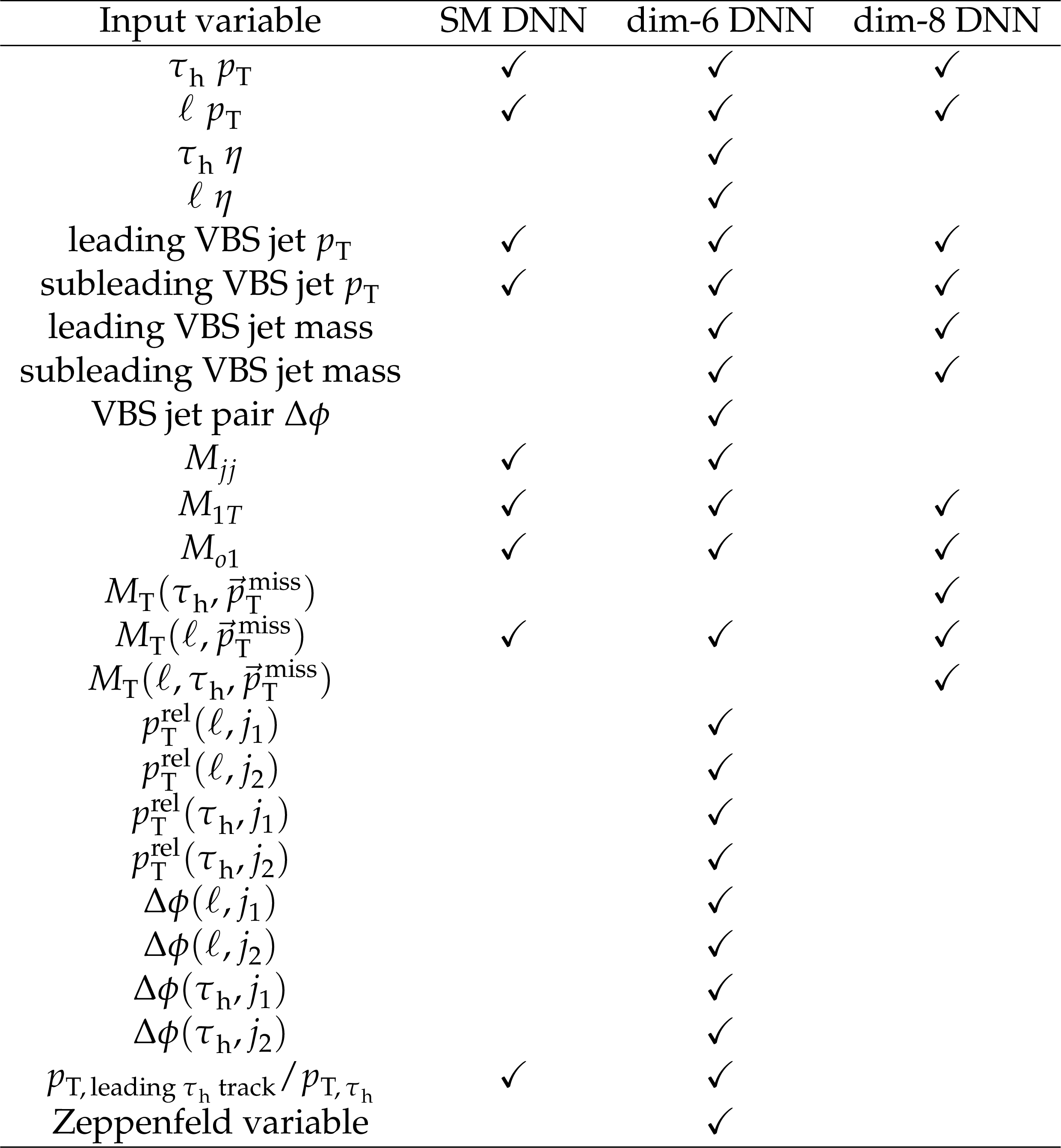
Additional Table 1:
Because of the large background and complex signal topology, sets of significant features (reported below) to separate signals and backgrounds are combined in three machine-learning discriminators, depending on which signal is targeted by the model. The discriminators are the outputs of feed-forward deep neural networks (DNNs). The three DNN models are devised to separate the SM VBS (SM DNN), EFT dim-6 (dim-6 DNN), and EFT dim-8 (dim-8 DNN) against the competitive SM background processes.\\ Among these variables, $ p_{\mathrm{T}}^{\text{rel}}(\ell, \mathrm{j})$ represents the component of the $ \ell $ or $ \tau_\mathrm{h} $ momentum $ \vec{p}_{\mathrm{l}} $ perpendicular to the momentum $ \vec{p}_{j} $ of VBS jet $ j $, while $ M_{\mathrm{T}} $(\ell, $ \tau_\mathrm{h} $, $ {\vec p}_{\mathrm{T}}^{\kern1pt\text{miss}} $) is defined considering the $\ell$ and the $ \tau_\mathrm{h} $ as a unique visible object, obtained by summing up their four-momenta. |
png pdf |
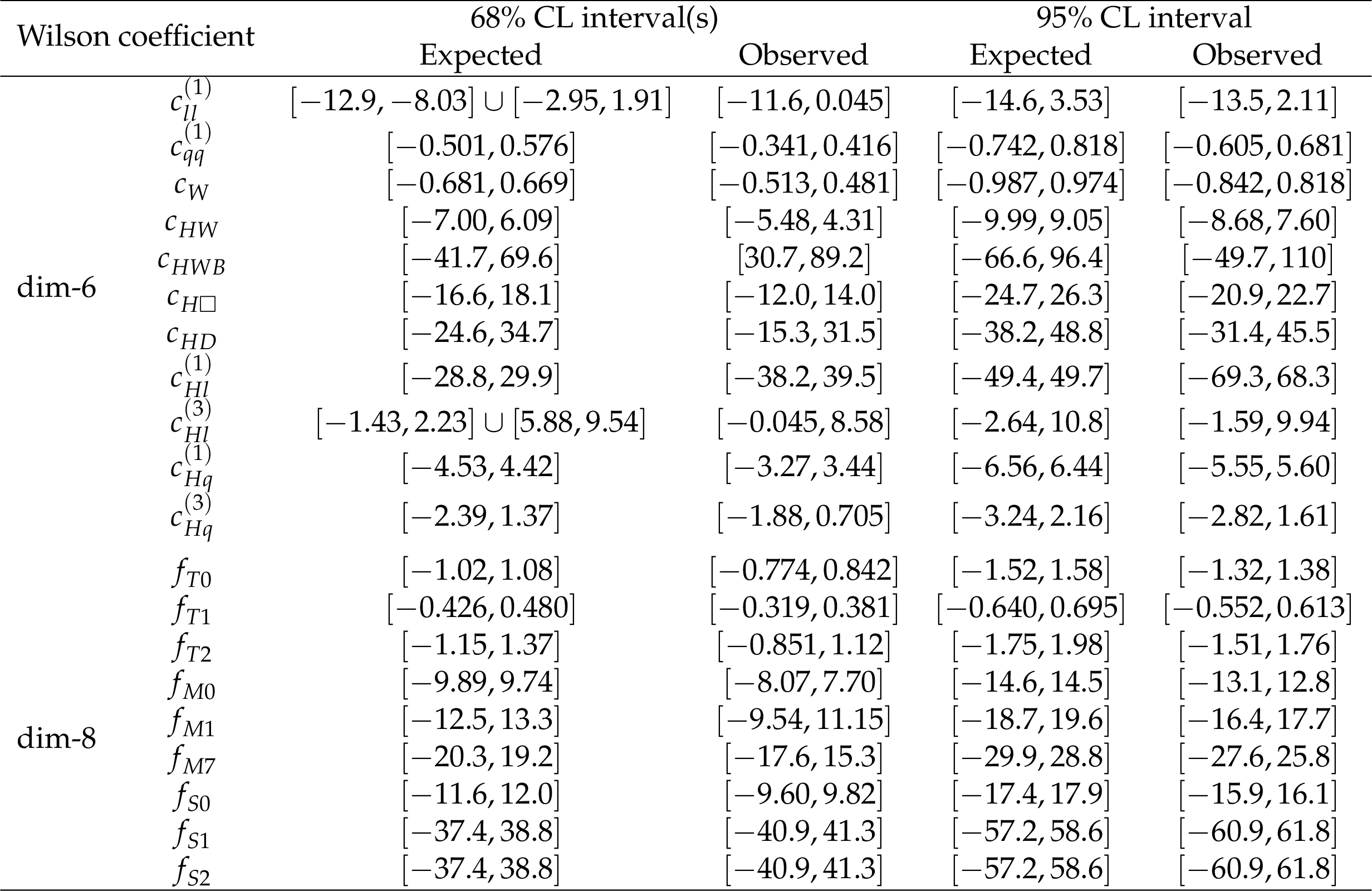
Additional Table 2:
Constraints on each EFT Wilson coefficient, derived from likelihood scans in which all other coefficients are fixed to zero. Results are given for both dim-6 and dim-8 operators, using fits to the output distributions of the EFT dim-6 and dim-8 discriminators, respectively. |
| References | ||||
| 1 | ATLAS and CMS Collaborations | Measurements of the Higgs boson production and decay rates and constraints on its couplings from a combined ATLAS and CMS analysis of the LHC pp collision data at $ \sqrt{s}= $ 7 and 8 TeV | JHEP 08 (2016) 45 | 1606.02266 |
| 2 | P. W. Higgs | Broken symmetries, massless particles and gauge fields | PL 12 (1964) 132 | |
| 3 | P. W. Higgs | Broken Symmetries and the Masses of Gauge Bosons | PRL 13 (1964) 508 | |
| 4 | F. Englert and R. Brout | Broken symmetry and the mass of gauge vector mesons | PRL 13 (1964) 321 | |
| 5 | W. Kilian, T. Ohl, J. Reuter, and M. Sekulla | High-Energy Vector Boson Scattering after the Higgs Discovery | PRD 91 (2015) 96007 | 1408.6207 |
| 6 | C. Garcia-Garcia, M. Herrero, and R. A. Morales | Unitarization effects in EFT predictions of WZ scattering at the LHC | PRD 100 (2019) 96003 | 1907.06668 |
| 7 | ATLAS Collaboration | Evidence for Electroweak Production of $ W^{\pm}W^{\pm}jj $ in $ pp $ Collisions at $ \sqrt{s}= $ 8 TeV with the ATLAS Detector | PRL 113 (2014) 141803 | 1405.6241 |
| 8 | CMS Collaboration | Observation of Electroweak Production of Same-Sign $ W $ Boson Pairs in the Two Jet and Two Same-Sign Lepton Final State in Proton-Proton Collisions at $ \sqrt{s}=13\text{ }\text{ }\mathrm{TeV} $ | PRL 120 (2018) 081801 | |
| 9 | CMS Collaboration | Search for anomalous electroweak production of vector boson pairs in association with two jets in proton-proton collisions at 13 TeV | PLB 798 (2019) 134985 | CMS-SMP-18-006 1905.07445 |
| 10 | CMS Collaboration | Evidence for electroweak production of four charged leptons and two jets in proton-proton collisions at $ \sqrt {s} $ = 13 TeV | PLB 812 (2021) 135992 | CMS-SMP-20-001 2008.07013 |
| 11 | CMS Collaboration | The CMS experiment at the CERN LHC | JINST 3 (2008) 8004 | |
| 12 | CMS Collaboration | Description and performance of track and primary-vertex reconstruction with the CMS tracker | JINST 9 (2014) 10009 | CMS-TRK-11-001 1405.6569 |
| 13 | CMS Tracker Group Collaboration | The CMS phase-1 pixel detector upgrade | JINST 16 (2021) 2027 | 2012.14304 |
| 14 | CMS Collaboration | Track impact parameter resolution for the full pseudo rapidity coverage in the 2017 dataset with the CMS phase-1 pixel detector | CMS Detector Performance Summary CMS-DP-2020-049, 2020 CDS |
|
| 15 | CMS Collaboration | The CMS trigger system | JINST 12 (2017) 1020 | CMS-TRG-12-001 1609.02366 |
| 16 | CMS Collaboration | Measurements of production cross sections of WZ and same-sign WW boson pairs in association with two jets in proton-proton collisions at $ \sqrt{s} = $ 13 TeV | PLB 809 (2020) 135710 | CMS-SMP-19-012 2005.01173 |
| 17 | B. Biedermann, A. Denner, and M. Pellen | Large electroweak corrections to vector-boson scattering at the Large Hadron Collider | PRL 118 (2017) 261801 | 1611.02951 |
| 18 | B. Biedermann, A. Denner, and M. Pellen | Complete NLO corrections to W$ ^{+} $W$ ^{+} $ scattering and its irreducible background at the LHC | JHEP 10 (2017) 124 | 1708.00268 |
| 19 | NNPDF Collaboration | Parton distributions from high-precision collider data | EPJC 77 (2017) 663 | 1706.00428 |
| 20 | C. Bierlich et al. | A comprehensive guide to the physics and usage of PYTHIA 8.3 | SciPost Phys. Codebases 8, 2022 link |
2203.11601 |
| 21 | CMS Collaboration | Extraction and validation of a new set of CMS PYTHIA8 tunes from underlying-event measurements | EPJC 80 (2020) 4 | CMS-GEN-17-001 1903.12179 |
| 22 | GEANT4 Collaboration | GEANT4: A Simulation toolkit | NIM A 506 (2003) 250 | |
| 23 | CMS Collaboration | Particle-flow reconstruction and global event description with the CMS detector | JINST 12 (2017) 3 | CMS-PRF-14-001 1706.04965 |
| 24 | CMS Collaboration | Commissioning of the Particle-Flow Event Reconstruction with the first LHC collisions recorded in the CMS detector | CMS PAS PFT-10-001, CERN, 2010 CMS-PAS-PFT-10-001 |
|
| 25 | M. Cacciari, G. P. Salam, and G. Soyez | The anti-$ k_t $ jet clustering algorithm | JHEP 04 (2008) 63 | 0802.1189 |
| 26 | M. Cacciari, G. P. Salam, and G. Soyez | FastJet user manual | EPJC 72 (2012) 1896 | 1111.6097 |
| 27 | M. Cacciari and G. P. Salam | Pileup subtraction using jet areas | PLB 659 (2008) 119 | 0707.1378 |
| 28 | CMS Collaboration | Technical proposal for the Phase-II upgrade of the Compact Muon Solenoid | CMS Technical Proposal CERN-LHCC-2015-010, CMS-TDR-15-02, 2015 CDS |
|
| 29 | CMS Collaboration | Performance of reconstruction and identification of $ \tau $ leptons decaying to hadrons and $ \nu_\tau $ in pp collisions at $ \sqrt{s}= $ 13 TeV | JINST 13 (2018) 5 | CMS-TAU-16-003 1809.02816 |
| 30 | CMS Collaboration | Measurement of Higgs Boson Production and Properties in the WW Decay Channel with Leptonic Final States | JHEP 01 (2014) 96 | CMS-HIG-13-023 1312.1129 |
| 31 | A. J. Barr et al. | Guide to transverse projections and mass-constraining variables | PRD 84 (2011) 95031 | 1105.2977 |
| 32 | D. P. Kingma and J. Ba | Adam: A method for stochastic optimization | Proceedings of the 3rd International Conference for Learning Representations, San Diego, 2017 link |
1412.6980 |
| 33 | I. Goodfellow, Y. Bengio, and A. Courville | Deep Learning | MIT Press, 2016 link |
|
| 34 | J. Fan, C. Zhang, and J. Zhang | Generalized likelihood ratio statistics and wilks phenomenon | The Annals of Statistics 2 (2000) 153 | |
| 35 | CMS Collaboration | Precision luminosity measurement in proton-proton collisions at $ \sqrt{s}= $ 13 TeV in 2015 and 2016 at CMS | EPJC 81 (2021) 800 | CMS-LUM-17-003 2104.01927 |
| 36 | CMS Collaboration | CMS luminosity measurement for the 2017 data-taking period at $ \sqrt{s}= $ 13 TeV | CMS Physics Analysis Summary, 2018 CMS-PAS-LUM-17-004 |
CMS-PAS-LUM-17-004 |
| 37 | CMS Collaboration | CMS luminosity measurement for the 2018 data-taking period at $ \sqrt{s}= $ 13 TeV | CMS Physics Analysis Summary, 2019 CMS-PAS-LUM-18-002 |
CMS-PAS-LUM-18-002 |
| 38 | A. Kalogeropoulos and J. Alwall | The SysCalc code: A tool to derive theoretical systematic uncertainties | 1801.08401 | |
| 39 | J. Butterworth et al. | PDF4LHC recommendations for LHC Run II | Journal of Physics G: , no.~2, 23001, 2016 Nuclear and Particle Physics 43 (2016) |
1510.03865 |
| 40 | CMS Collaboration | Jet energy scale and resolution in the CMS experiment in pp collisions at 8 TeV | JINST 12 (2017) 2 | CMS-JME-13-004 1607.03663 |
|
|
Compact Muon Solenoid LHC, CERN |
|

|

|

|

|

|