

Compact Muon Solenoid
LHC, CERN
| CMS-PAS-TOP-16-013 | ||
| Measurement of the ${\rm t}{\rm \bar{t}}$ production cross section at 13 TeV in the all-jets final state | ||
| CMS Collaboration | ||
| June 2016 | ||
| Abstract: The top quark pair production cross section is measured in the all-jets decay channel using pp collisions at a centre-of-mass energy of 13 TeV at the LHC with the CMS detector. The data sample corresponds to an integrated luminosity of 2.53 fb$^{-1}$ recorded in 2015. The inclusive ${\rm t}{\rm \bar{t}}$ production cross section is measured to be 834 $\pm$ 25 (stat) $_{-104}^{+118}$ (syst) $\pm$ 23 (lumi) pb. Differential cross sections at detector level are measured as a function of the leading top quark transverse momentum, $p_{\rm T}$, and are compared to predictions from quantum chromodynamics. The spectrum is constructed by combining two distinct reconstruction approaches, targeting the low $p_{\rm T}$ (resolved top quark decay products), and the high $p_{\rm T}$ (boosted top quark decay products) regions. Finally, the cross sections are also reported at parton level, extrapolated to the full phase space. In all cases, the measured top quark $p_{\rm T}$ spectrum is found to be significantly softer than the theory predictions. | ||
| Links: CDS record (PDF) ; inSPIRE record ; CADI line (restricted) ; | ||
| Figures | |

png pdf |
Figure 1-a:
a: Reconstructed ${m_\mathrm {t}}$ in the resolved analysis before and after the kinematic fit for the most probable combination of jets (from the kinematic fit) in $\mathrm{ t \bar{t} } $ simulated events. b: Softdrop mass $m_{\rm SD}$ for the leading jet, before (solid line) and after (dashed line) the requirement of at least one b-tagged subjet, in $\mathrm{ t \bar{t} } $ simulated events. |

png pdf |
Figure 1-b:
a: Reconstructed ${m_\mathrm {t}}$ in the resolved analysis before and after the kinematic fit for the most probable combination of jets (from the kinematic fit) in $\mathrm{ t \bar{t} } $ simulated events. b: Softdrop mass $m_{\rm SD}$ for the leading jet, before (solid line) and after (dashed line) the requirement of at least one b-tagged subjet, in $\mathrm{ t \bar{t} } $ simulated events. |

png pdf |
Figure 2-a:
a: Postfit ${m_\mathrm {t}}$ distribution in the resolved selection (without the ${m_\mathrm {t}}$ cut). The QCD background is taken from the control sample and the $\mathrm{ t \bar{t} } $ signal from the simulation. The distributions are normalized to the fitted yields. The vertical dashed lines indicate the ${m_\mathrm {t}}$ cut (150-200 GeV) applied to all other observables. b: Postfit $\Delta R_{\rm bb}$ distribution in the resolved selection (including the ${m_\mathrm {t}}$ cut). The distributions are normalized to the fitted yields corrected with the signal and background fractions within the ${m_\mathrm {t}}$ window, while the shaded band shows the fit uncertainty. The bottom panels show the fractional difference between the data and the sum of $\mathrm{ t \bar{t} } $ signal plus background event yield. |

png pdf |
Figure 2-b:
a: Postfit ${m_\mathrm {t}}$ distribution in the resolved selection (without the ${m_\mathrm {t}}$ cut). The QCD background is taken from the control sample and the $\mathrm{ t \bar{t} } $ signal from the simulation. The distributions are normalized to the fitted yields. The vertical dashed lines indicate the ${m_\mathrm {t}}$ cut (150-200 GeV) applied to all other observables. b: Postfit $\Delta R_{\rm bb}$ distribution in the resolved selection (including the ${m_\mathrm {t}}$ cut). The distributions are normalized to the fitted yields corrected with the signal and background fractions within the ${m_\mathrm {t}}$ window, while the shaded band shows the fit uncertainty. The bottom panels show the fractional difference between the data and the sum of $\mathrm{ t \bar{t} } $ signal plus background event yield. |

png pdf |
Figure 3-a:
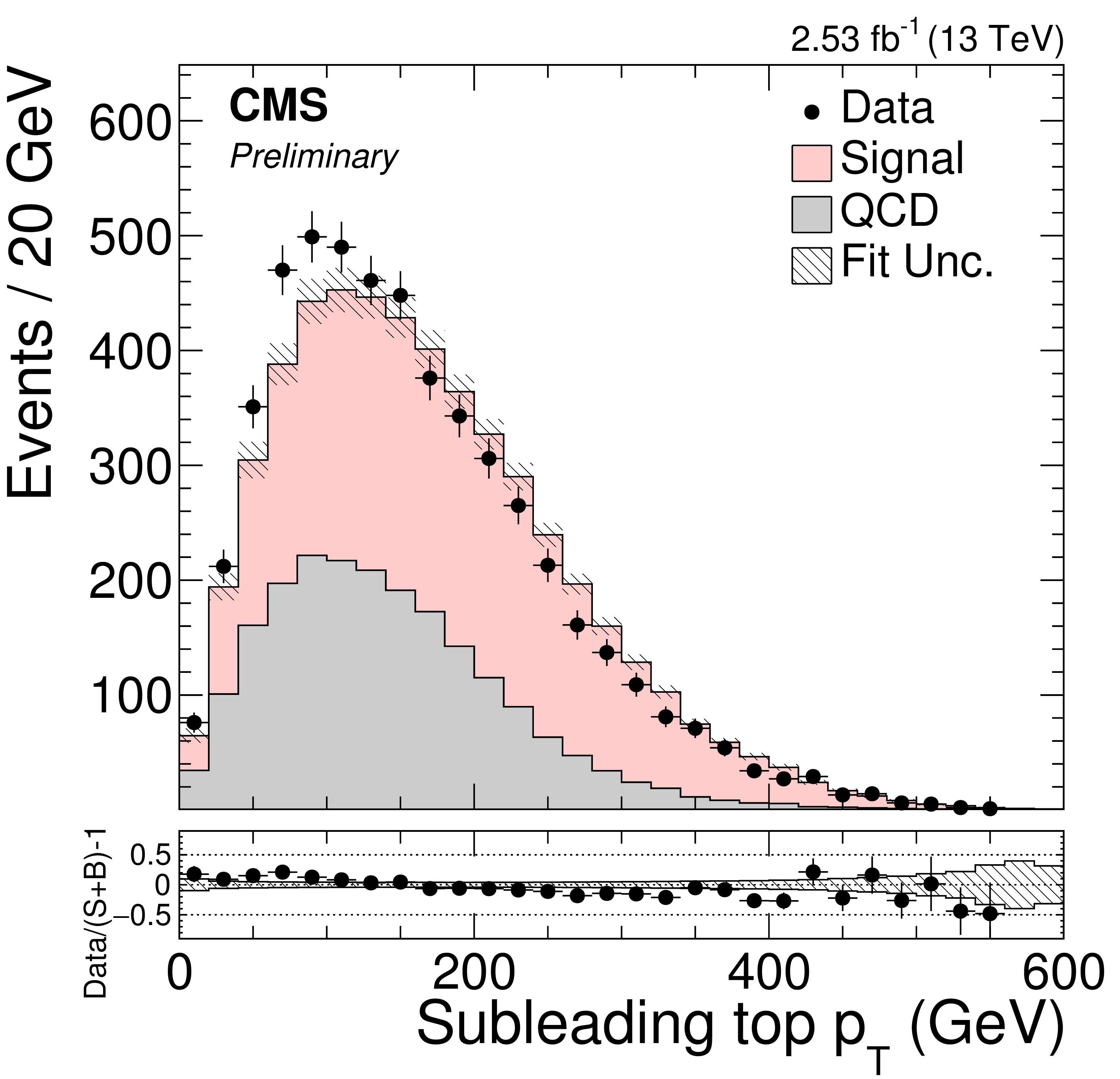
Postfit distributions of the ${p_{\mathrm {T}}}$ of the leading (left) and subleading (right) top quarks in the full resolved selection (including the ${m_\mathrm {t}}$ cut). The QCD background is taken from the control sample and the $\mathrm{ t \bar{t} } $ signal from the simulation. The distributions are normalized to the fitted yields corrected with the signal and background fractions within the ${m_\mathrm {t}}$ window, while the shaded band shows the fit uncertainty. The bottom panels show the fractional difference between the data and the sum of $\mathrm{ t \bar{t} } $ signal plus background event yield. |
png pdf |
Figure 3-b:
Postfit distributions of the ${p_{\mathrm {T}}}$ of the leading (left) and subleading (right) top quarks in the full resolved selection (including the ${m_\mathrm {t}}$ cut). The QCD background is taken from the control sample and the $\mathrm{ t \bar{t} } $ signal from the simulation. The distributions are normalized to the fitted yields corrected with the signal and background fractions within the ${m_\mathrm {t}}$ window, while the shaded band shows the fit uncertainty. The bottom panels show the fractional difference between the data and the sum of $\mathrm{ t \bar{t} } $ signal plus background event yield. |

png pdf |
Figure 4-a:
a: Postfit $m_\text {SD}$ distribution of the leading jet in the boosted selection (without the ${m_\mathrm {t}}$ cut). The QCD background is taken from the control sample and the $\mathrm{ t \bar{t} } $ signal from the simulation. The distributions are normalized to the fitted yields. The vertical dashed lines indicate the $m_\text {SD}$ cut (150-200 GeV) applied for all other observables. b: Postfit $m_\text {SD}$ distribution of the second jet in the boosted selection (including the $m_\text {SD}$ cut). The distributions are normalized to the fitted yields corrected with the signal and background fractions within the $m_\text {SD}$ window, while the shaded band shows the fit uncertainty. The bottom panels show the fractional difference between the data and the sum of $\mathrm{ t \bar{t} } $ signal plus background event yield. |

png pdf |
Figure 4-b:
a: Postfit $m_\text {SD}$ distribution of the leading jet in the boosted selection (without the ${m_\mathrm {t}}$ cut). The QCD background is taken from the control sample and the $\mathrm{ t \bar{t} } $ signal from the simulation. The distributions are normalized to the fitted yields. The vertical dashed lines indicate the $m_\text {SD}$ cut (150-200 GeV) applied for all other observables. b: Postfit $m_\text {SD}$ distribution of the second jet in the boosted selection (including the $m_\text {SD}$ cut). The distributions are normalized to the fitted yields corrected with the signal and background fractions within the $m_\text {SD}$ window, while the shaded band shows the fit uncertainty. The bottom panels show the fractional difference between the data and the sum of $\mathrm{ t \bar{t} } $ signal plus background event yield. |

png pdf |
Figure 5-a:
Postfit distributions of the Fisher discriminant (a) and of the ${p_{\mathrm {T}}}$ of the leading (b) and subleading (c) top quarks in the boosted selection (including the $m_\text {SD}$ cut). The QCD background is taken from the control sample and the $\mathrm{ t \bar{t} } $ signal from the simulation. The distributions are normalized to the fitted yields corrected with the signal and background fractions within the ${m_\mathrm {t}}$ window, while the shaded band shows the fit uncertainty. The bottom panels show the fractional difference between the data and the sum of $\mathrm{ t \bar{t} } $ signal plus background event yield. |

png pdf |
Figure 5-b:
Postfit distributions of the Fisher discriminant (a) and of the ${p_{\mathrm {T}}}$ of the leading (b) and subleading (c) top quarks in the boosted selection (including the $m_\text {SD}$ cut). The QCD background is taken from the control sample and the $\mathrm{ t \bar{t} } $ signal from the simulation. The distributions are normalized to the fitted yields corrected with the signal and background fractions within the ${m_\mathrm {t}}$ window, while the shaded band shows the fit uncertainty. The bottom panels show the fractional difference between the data and the sum of $\mathrm{ t \bar{t} } $ signal plus background event yield. |

png pdf |
Figure 5-c:
Postfit distributions of the Fisher discriminant (a) and of the ${p_{\mathrm {T}}}$ of the leading (b) and subleading (c) top quarks in the boosted selection (including the $m_\text {SD}$ cut). The QCD background is taken from the control sample and the $\mathrm{ t \bar{t} } $ signal from the simulation. The distributions are normalized to the fitted yields corrected with the signal and background fractions within the ${m_\mathrm {t}}$ window, while the shaded band shows the fit uncertainty. The bottom panels show the fractional difference between the data and the sum of $\mathrm{ t \bar{t} } $ signal plus background event yield. |

png pdf |
Figure 6-a:
Postfit jet substructure distributions in the boosted selection (including the $m_\text {SD}$ cut): $\tau _3/\tau _1$ (a,b), $\tau _3/\tau _2$ (c,d), for the leading (a,c) and subleading (b,d) jet; also shown (e,f) is the leading (e) or subleading (f) subjet mass of the leading jet. The QCD background is taken from the control sample and the $\mathrm{ t \bar{t} } $ signal from the simulation. The distributions are normalized to the fitted yields corrected with the signal and background fractions within the $m_\text {SD}$ window, while the shaded band shows the fit uncertainty. The bottom panels show the fractional difference between the data and the sum of $\mathrm{ t \bar{t} } $ signal plus background event yield. |

png pdf |
Figure 6-b:
Postfit jet substructure distributions in the boosted selection (including the $m_\text {SD}$ cut): $\tau _3/\tau _1$ (a,b), $\tau _3/\tau _2$ (c,d), for the leading (a,c) and subleading (b,d) jet; also shown (e,f) is the leading (e) or subleading (f) subjet mass of the leading jet. The QCD background is taken from the control sample and the $\mathrm{ t \bar{t} } $ signal from the simulation. The distributions are normalized to the fitted yields corrected with the signal and background fractions within the $m_\text {SD}$ window, while the shaded band shows the fit uncertainty. The bottom panels show the fractional difference between the data and the sum of $\mathrm{ t \bar{t} } $ signal plus background event yield. |
png pdf |
Figure 6-c:
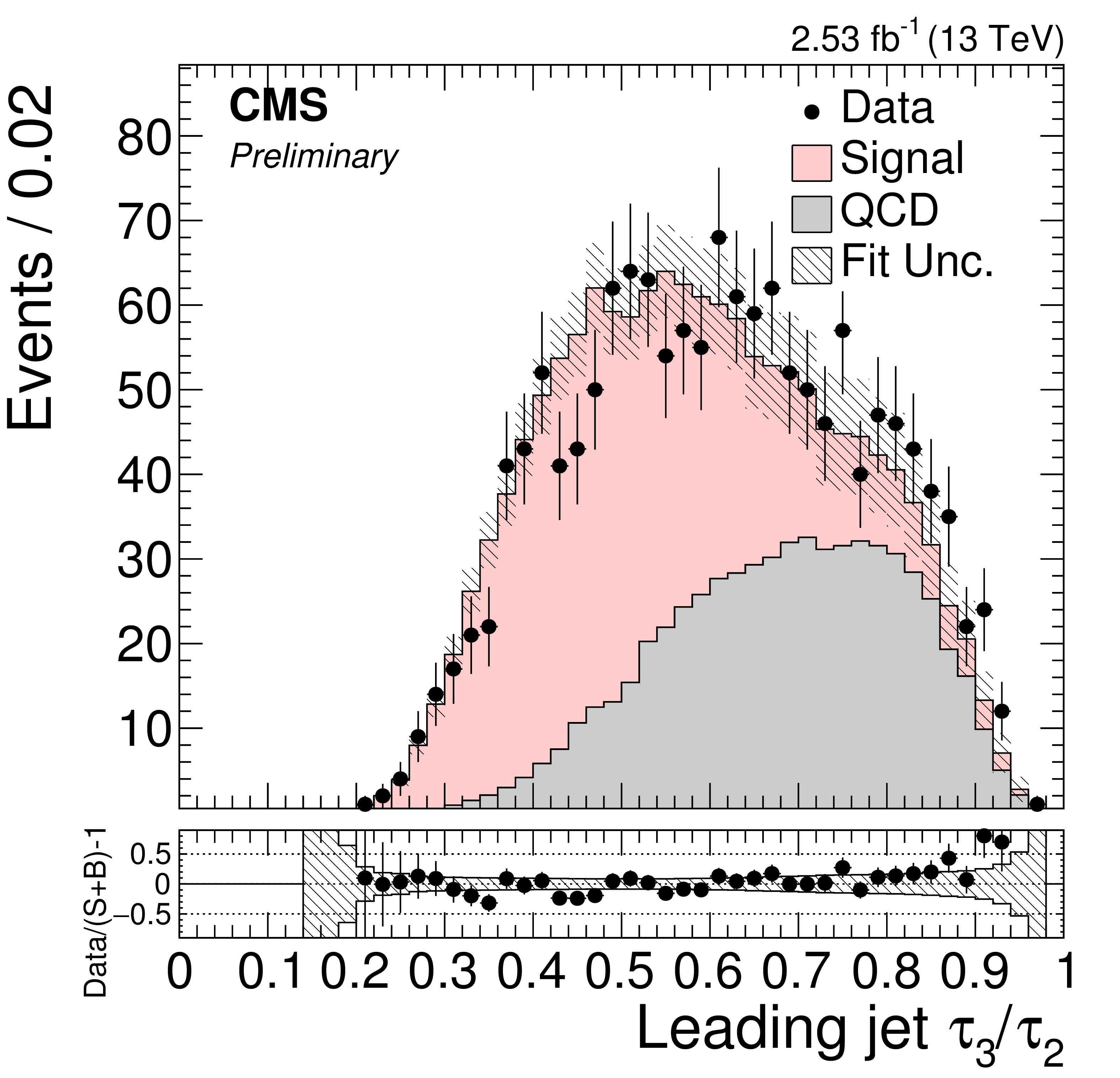
Postfit jet substructure distributions in the boosted selection (including the $m_\text {SD}$ cut): $\tau _3/\tau _1$ (a,b), $\tau _3/\tau _2$ (c,d), for the leading (a,c) and subleading (b,d) jet; also shown (e,f) is the leading (e) or subleading (f) subjet mass of the leading jet. The QCD background is taken from the control sample and the $\mathrm{ t \bar{t} } $ signal from the simulation. The distributions are normalized to the fitted yields corrected with the signal and background fractions within the $m_\text {SD}$ window, while the shaded band shows the fit uncertainty. The bottom panels show the fractional difference between the data and the sum of $\mathrm{ t \bar{t} } $ signal plus background event yield. |
png pdf |
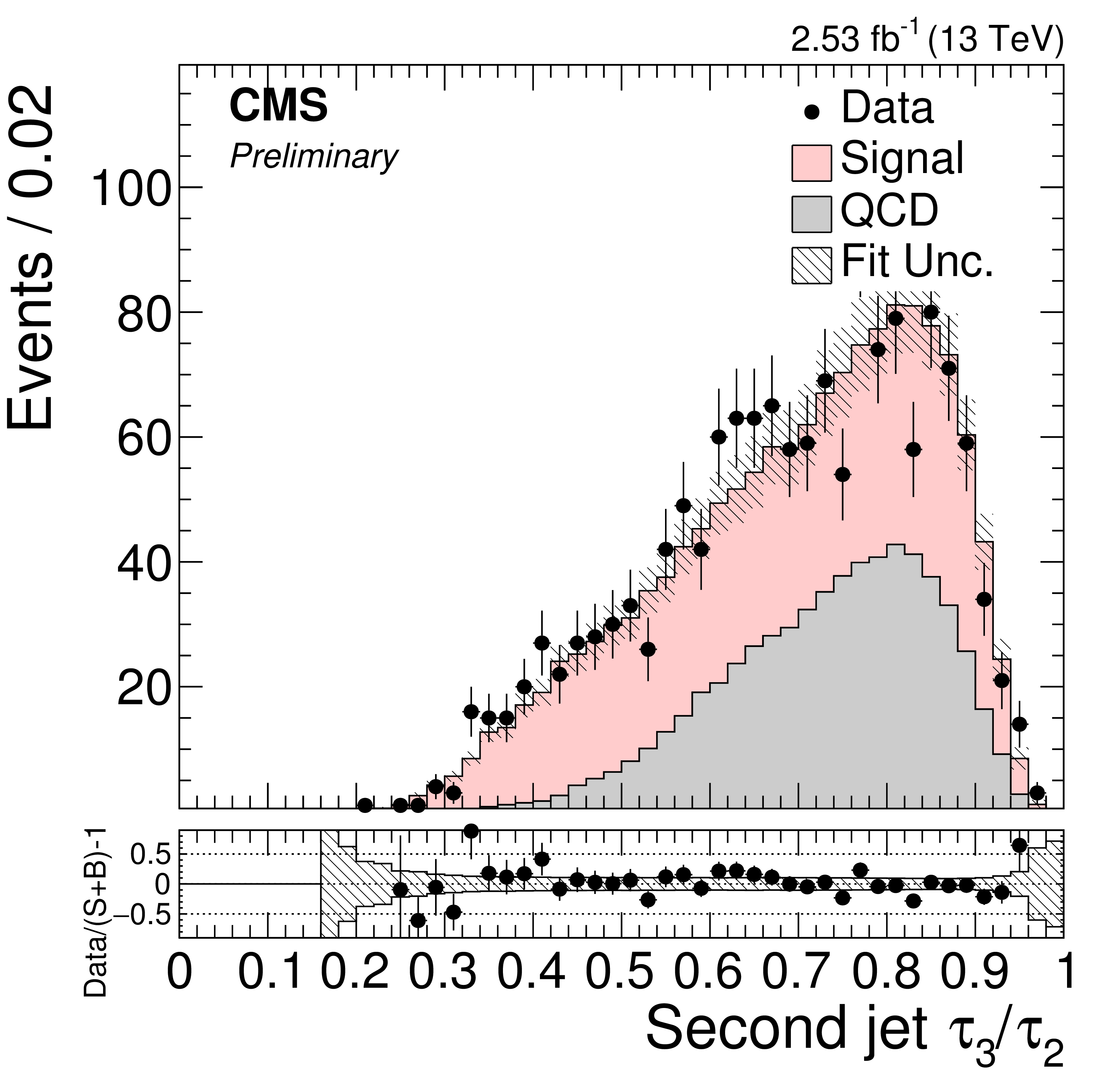
Figure 6-d:
Postfit jet substructure distributions in the boosted selection (including the $m_\text {SD}$ cut): $\tau _3/\tau _1$ (a,b), $\tau _3/\tau _2$ (c,d), for the leading (a,c) and subleading (b,d) jet; also shown (e,f) is the leading (e) or subleading (f) subjet mass of the leading jet. The QCD background is taken from the control sample and the $\mathrm{ t \bar{t} } $ signal from the simulation. The distributions are normalized to the fitted yields corrected with the signal and background fractions within the $m_\text {SD}$ window, while the shaded band shows the fit uncertainty. The bottom panels show the fractional difference between the data and the sum of $\mathrm{ t \bar{t} } $ signal plus background event yield. |

png pdf |
Figure 6-e:
Postfit jet substructure distributions in the boosted selection (including the $m_\text {SD}$ cut): $\tau _3/\tau _1$ (a,b), $\tau _3/\tau _2$ (c,d), for the leading (a,c) and subleading (b,d) jet; also shown (e,f) is the leading (e) or subleading (f) subjet mass of the leading jet. The QCD background is taken from the control sample and the $\mathrm{ t \bar{t} } $ signal from the simulation. The distributions are normalized to the fitted yields corrected with the signal and background fractions within the $m_\text {SD}$ window, while the shaded band shows the fit uncertainty. The bottom panels show the fractional difference between the data and the sum of $\mathrm{ t \bar{t} } $ signal plus background event yield. |

png pdf |
Figure 6-f:
Postfit jet substructure distributions in the boosted selection (including the $m_\text {SD}$ cut): $\tau _3/\tau _1$ (a,b), $\tau _3/\tau _2$ (c,d), for the leading (a,c) and subleading (b,d) jet; also shown (e,f) is the leading (e) or subleading (f) subjet mass of the leading jet. The QCD background is taken from the control sample and the $\mathrm{ t \bar{t} } $ signal from the simulation. The distributions are normalized to the fitted yields corrected with the signal and background fractions within the $m_\text {SD}$ window, while the shaded band shows the fit uncertainty. The bottom panels show the fractional difference between the data and the sum of $\mathrm{ t \bar{t} } $ signal plus background event yield. |

png pdf |
Figure 7-a:
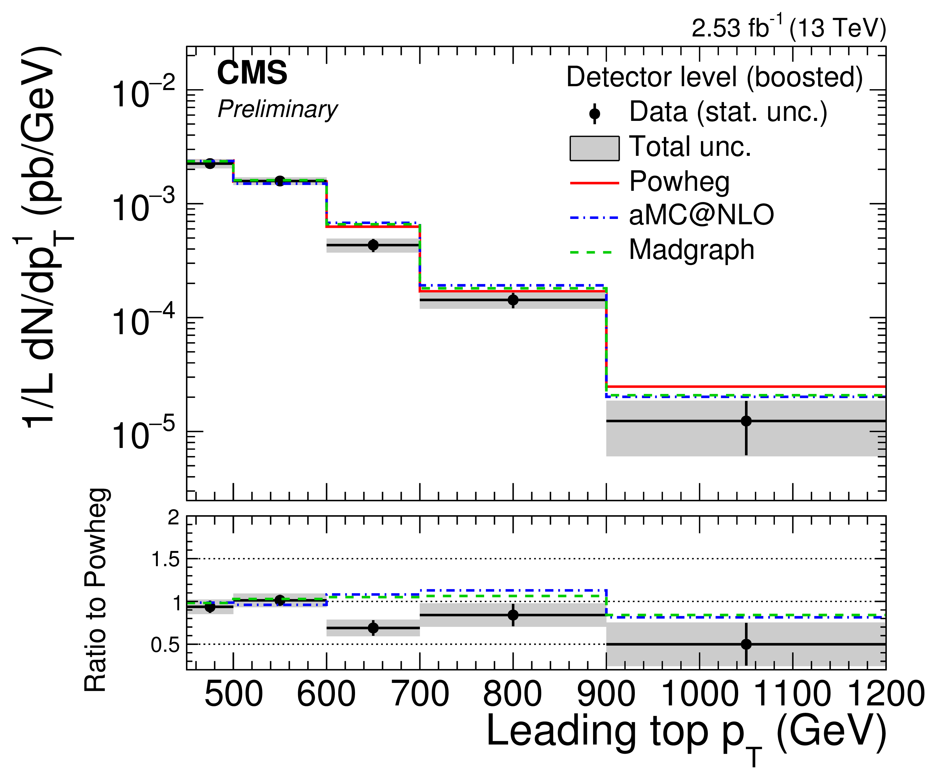
Differential $\mathrm{ t \bar{t} } $ cross section as a function of the leading top quark ${p_{\mathrm {T}}}$ at detector level in the resolved (left) and the boosted (right) analysis. The bottom panel shows the ratio to the default simulation POWHEG + PYTHIA8. |
png pdf |
Figure 7-b:
Differential $\mathrm{ t \bar{t} } $ cross section as a function of the leading top quark ${p_{\mathrm {T}}}$ at detector level in the resolved (left) and the boosted (right) analysis. The bottom panel shows the ratio to the default simulation POWHEG + PYTHIA8. |

png pdf |
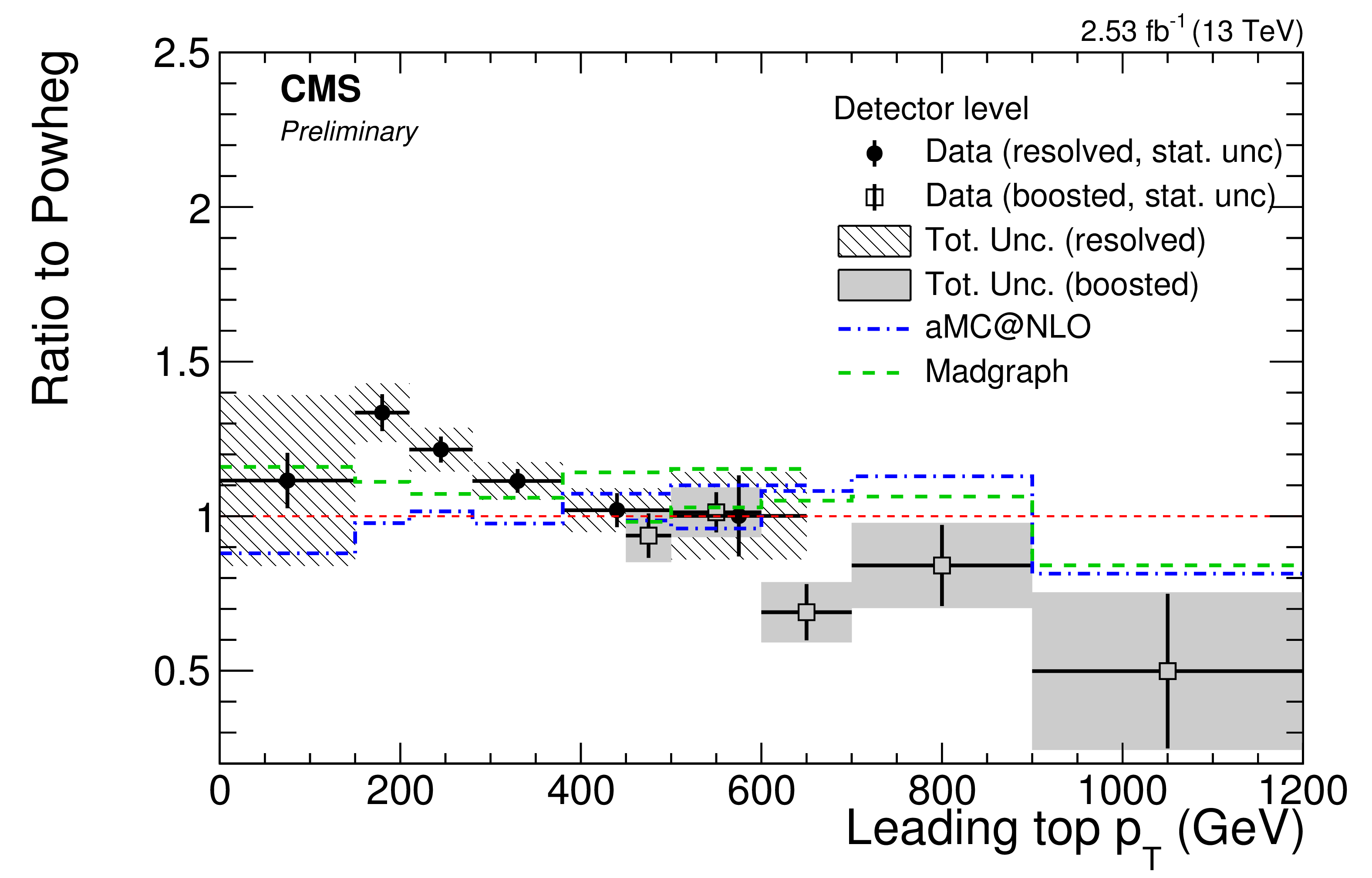
Figure 8-a:
a: Differential $\mathrm{ t \bar{t} } $ cross section as a function of the leading top quark ${p_{\mathrm {T}}}$ at detector level in the resolved and boosted analyses. b: Ratio of the differential $\mathrm{ t \bar{t} } $ cross sections over the default simulation POWHEG + PYTHIA8. |
png pdf |
Figure 8-b:
a: Differential $\mathrm{ t \bar{t} } $ cross section as a function of the leading top quark ${p_{\mathrm {T}}}$ at detector level in the resolved and boosted analyses. b: Ratio of the differential $\mathrm{ t \bar{t} } $ cross sections over the default simulation POWHEG + PYTHIA8. |

png pdf |
Figure 9-a:
a: Unfolded differential cross section, extrapolated to the full phase space, as a function of the leading top quark ${p_{\mathrm {T}}} $. b: Ratio of the unfolded differential cross section, extrapolated to the full phase space, over the POWHEG + PYTHIA8 prediction. |

png pdf |
Figure 9-b:
a: Unfolded differential cross section, extrapolated to the full phase space, as a function of the leading top quark ${p_{\mathrm {T}}} $. b: Ratio of the unfolded differential cross section, extrapolated to the full phase space, over the POWHEG + PYTHIA8 prediction. |
| Tables | |

png pdf |
Table 1:
Summary of the resolved and boosted event selections. |

png pdf |
Table 2:
Fractional uncertainties on the inclusive $\mathrm{ t \bar{t} } $ production cross section as measured in the resolved and boosted analyses. |
| Summary |
| A measurement has been presented of the $\mathrm{ t \bar{t} }$ production cross section, both inclusively, and differentially, as a function of the leading top quark $p_\mathrm{ T }$, in the all-jets final state. In order to cover the full available phase space, two separate analyses methods have been used: the resolved one, targeting the low-$p_\mathrm{ T }$ range, where the top quark decay products can be reconstructed separately, and the boosted one, targeting the high-$p_\mathrm{ T }$ range, where the top quark decay products are clustered as a single object. The inclusive cross section has been measured to be 834 $\pm$ 25 (stat) $_{-104}^{+118}$ (syst) $\pm$ 23 (lumi) pb, in agreement with the theory prediction, and other CMS measurements in different channels [29,30]. For the first time, the differential measurement is reported up to $p_\mathrm{ T }= $ 1.2 TeV in the all-jets final state, by combining the two analysis methods, at detector level and in the full partonic phase space. The two methods agree well in the small overlapping region around $p_\mathrm{ T }\sim $ 550 GeV. Comparisons with LO and NLO MC indicate strongly that the measured spectrum is falling more steeply than the theory predictions, an observation which is consistent with measurements performed with the dilepton and lepton+jets final states at 7, 8, and 13 TeV. |
|
|
Compact Muon Solenoid LHC, CERN |
|

|

|

|

|

|